Overlapping Schwarz Preconditioners for Isogeometric Collocation Methods Based on Generalized B-Splines

Abstract

We study overlapping additive Schwarz (OAS) preconditioners for the solution of elliptic boundary value problems discretized using isogeometric collocation methods based on generalized B-splines (GB-splines). Through a series of numerical experiments, we demonstrate the scalability of the proposed preconditioning strategy with respect to the number of subdomains, as well as its robustness with respect to the parameters of the isogeometric discretization.

1. Introduction

Isogeometric Analysis (IGA) is a modern numerical framework for the solution of partial differential equations (PDEs), originally introduced in [1] (see also [2] for a detailed overview). The primary objective of IGA is to bridge the gap between Computer-Aided Design (CAD) and numerical PDE solvers. Within this framework, Non-Uniform Rational B-splines (NURBS), which are employed in CAD to represent geometries, are also used to discretize the unknowns of the PDE, following the isoparametric concept [3,4].

While NURBS offer the capability to exactly represent a broad class of conic section geometries, they are inherently incapable of describing transcendental curves, such as cycloids, helices, and catenaries. In addition, the rational nature of NURBS introduces significant complexity in the processes of exact differentiation and integration. To overcome these limitations, Generalized B-splines (GB-splines) have been proposed and systematically investigated [5,6,7].

While standard polynomial B-splines are smooth piecewise functions confined to the algebraic polynomial space, GB-splines extend this concept by employing piecewise functions defined in a broader Tchebycheff space [8,9,10,11,12]. By incorporating carefully selected non-polynomial functions, GB-splines offer two major advantages: (i) improved properties for differentiation and integration, which are particularly beneficial in applications such as electromagnetism [7,13,14], and (ii) the ability to exactly represent not only conic sections but also other geometric shapes, commonly used in engineering applications. As a result, GB-splines have emerged as a compelling alternative to both polynomial B-splines and NURBS in computational modeling and simulation contexts [5,7]. Since then, they have been explored in various studies on isogeometric analysis [15,16], significantly impacting geometric modeling and numerical simulation [17].

In order to reduce the computational costs in IGA Galerkin (IGA-G) formulations, collocation methods have been incorporated in IGA (see, for instance, [18,19]). Indeed, the assembly of the collocation-based stiffness matrix requires only a single evaluation per basis function, and the resulting linear system is considerably sparser than that arising from IGA-G methods (see [20] for a comprehensive comparison). Isogeometric collocation (IGA-C) methods have demonstrated successful applications in various fields, such as beam analysis [21,22] and the Cahn–Hilliard problem [23]. Despite these computational advantages, IGA-C methods still lack a solid theoretical foundation in more than one dimension (see [18] for the convergence rates in the one-dimensional case).

In the analogy with the IGA-G approach based on GB-splines [24], the condition numbers of stiffness matrices arising in IGA-C methods based on GB-splines grow rapidly as either the mesh is refined or the GB-spline degree increases (see

Table 1. Condition numbers of IGA-C stiffness matrices based on GB-splines on the 2D square domain, with respect to the 2-norm as the function of h and of p, maximal regularity $k=p-1$.

IGA Collocation Stiffness Matrices
h	p = 2	p = 3	p = 4
1/8	14.58	21.98	53.26
1/16	53.51	84.02	163.42
1/32	209.14	340.56	543.25
1/64	831.67	1383.08	2297.88
1/128	3321.74	5395.86	9836.58
1/256	13,282.02	21,281.60	37,613.05

for condition number details of the unpreconditioned system). Consequently, preconditioners become an essential tool to maintain the efficiency of IGA-C schemes (see, e.g., Figure 1 for the complex spectrum of the unpreconditioned operators and OAS preconditioned ones).

Preconditioners and domain decomposition (DD) methods have been extensively employed in IGA Galerkin schemes based on NURBS or GB-splines as shown in works, such as overlapping Schwarz methods [24,26,27,28,29,30], IETI (IGA equivalent of FETI) [31,32,33,34,35,36], BDDC [37], and BDDC deluxe [38,39,40,41] and multilevel solvers (BPX [42] and multigrid methods [43,44,45,46,47]). In a similar manner, preconditioning techniques in NURBS-based IGA collocation schemes have been explored (see, e.g., [28,48,49]). However, to the best of our knowledge, there are no results in the literature on preconditioners or DD methods for IGA collocation schemes based on GB-splines. Our contribution in the present paper is to present scalable Overlapping Additive Schwarz (OAS) DD methods for IGA collocation schemes based on GB-splines.

In this work, we consider the following model elliptic problem:

$$-\nabla ·\left(\rho \nabla u\right)=f\hspace{1em}\mathrm{in} \mathrm{\Omega },\hspace{1em}u=0\hspace{1em}\mathrm{on} \partial \mathrm{\Omega },$$

(1)

where the scalar function satisfies $0<{\rho }_{\min }\le \rho \le {\rho }_{\max }$ for all $x\in \mathrm{\Omega }$, and $\mathrm{\Omega }\subset {\mathbb{R}}^d$ represents a bounded and connected CAD domain. In a similar way to [24], where OAS preconditioners for IGA Galerkin schemes based on GB-splines were analyzed, we show through a series of numerical experiments that one-level preconditioners alone for IGA-C schemes based on GB-splines are not scalable, while a two-level OAS preconditioner incorporating a coarse problem ensures scalability. In particular, from numerical results, we study the behavior of our OAS preconditioners with respect to discretization parameters. Also, we test their performance in the presence of domain deformation.

The remainder of this paper is structured as follows: Section 2 introduces the definition and crucial properties of GB-splines in IGA. In Section 3, we describe the proposed overlapping Schwarz preconditioners. In Section 4 we present a set of numerical results in two and three spatial dimensions. Finally, we summarize our conclusions in Section 5.

2. Generalized B-Splines (GB-Splines)

2.1. Generalized Polynomial Spaces

Following Section 4 in [9], we first present the definition of GB-splines and outline their basic properties. Throughout this work, generalized B-splines serve as basis functions in Isogeometric Analysis (IGA) discretizations (see [7] for details).

Definition 1

([29]). Let $p\in \mathbb{N}$ with $p\ge 2$ and Δ a partition of the closed interval $[0,1]$ given by

$$∆:=\{0={\eta }_0<{\eta }_1<\cdots <{\eta }_{\ell +1}=1\},\hspace{1em}\ell \in \mathbb{N}.$$

(2)

A generalized polynomial space of degree p is defined as

$${\mathbb{GP}}_p^{U,V}(∆):=\langle 1,\zeta ,\dots ,{\zeta }^{p-2},U(\zeta ),V(\zeta )\rangle ,\hspace{1em}\zeta \in [{\eta }_0,{\eta }_{\ell +1}],$$

(3)

where $U,V$ are of class $C^p([{\eta }_i,{\eta }_{i+1}])$, and $\langle D^{p-1}U,D^{p-1}V\rangle$ is an extended Tchebycheff space on $[{\eta }_i,{\eta }_{i+1}]$ for all $0\le i\le \ell$.

Various forms of the generalized polynomial space ${\mathbb{GP}}_p^{U,V}(∆)$ are studied in [9] (see also [8,10,11] for a comprehensive discussion on Tchebycheff spaces). Popular options for the functions U and V on each subinterval $[{\eta }_i,{\eta }_{i+1}]$ include the following:

$${\mathbb{P}}_p([{\eta }_i,{\eta }_{i+1}]):=\langle 1,\zeta ,\dots ,{\zeta }^{p-2},{\zeta }^{p-1},{\zeta }^p\rangle ,$$

(4)

which corresponds to the space of standard polynomial B-splines;

$${\mathbb{E}}_{p,{\alpha }_i}([{\eta }_i,{\eta }_{i+1}]):=\langle 1,\zeta ,\dots ,{\zeta }^{p-2},e^{{\alpha }_i\zeta },e^{-{\alpha }_i\zeta }\rangle ,\hspace{1em}0<{\alpha }_i\in \mathbb{R},$$

(5)

which defines the space of exponential GB-splines;

$${\mathbb{T}}_{p,{\alpha }_i}([{\eta }_i,{\eta }_{i+1}]):=\langle 1,\zeta ,\dots ,{\zeta }^{p-2},\cos ({\alpha }_i\zeta ),\sin ({\alpha }_i\zeta )\rangle ,\hspace{1em}0<{\alpha }_i({\eta }_{i+1}-{\eta }_i)<\pi ,$$

(6)

which defines the space of trigonometric GB-splines.

2.2. Univariate GB-Splines

Following the IGA paradigm, let us consider $n,p\in \mathbb{N}$ with $p\ge 2$ and define a knot vector $\sum$ over the one-dimensional interval $[0,1]$, which is associated with the partition $∆$ given in (2):

$$\sum =\{{\xi }_1,{\xi }_2,\dots ,{\xi }_{n+p+1}\}=(\underset{{\mu }_0}{\underbrace{{\eta }_0,\dots ,{\eta }_0}},\dots ,\underset{{\mu }_{\ell +1}}{\underbrace{{\eta }_{\ell +1},\dots ,{\eta }_{\ell +1}}}),$$

(7)

for some positive integers ${\mu }_0,\dots ,{\mu }_{\ell +1}$ satisfying ${\sum }_{i=0}^{\ell +1}{\mu }_i=n+p+1$. Furthermore, we assume that the knot vector $\sum$ is a p-open knot vector interpolating at the endpoints of the parametric space $\widehat{I}:=(0,1)$:

$$0={\xi }_1=\cdots ={\xi }_{p+1}<\cdots <{\xi }_{n+1}=\cdots ={\xi }_{n+p+1}=1.$$

Now, we associate GB-splines of degree p with the knot vector $\sum$ and a generalized polynomial space ${\mathbb{GP}}_p^{U,V}(∆)$. We remark that $\sum$ and ${\mathbb{GP}}_p^{U,V}(∆)$ are both connected to the partition $∆$ as described in (2) (see [6,7,9,17] and the references therein).

Definition 2

([29]). Given a partition Δ, let ${\mathbb{GP}}_p^{U,V}(∆)$ be a generalized polynomial space of degree $p\ge 2$, and let Σ be a knot vector connected to Δ as in (7). For any ${\xi }_j<{\xi }_{j+1}$, let $u_j,v_j$ be the unique functions in $\langle D^{p-1}U,D^{p-1}V\rangle$ on $[{\xi }_j,{\xi }_{j+1}]$ satisfying

$$u_j({\xi }_j)=1,\hspace{1em}{u}_j({\xi }_{j+1})=0,\hspace{1em}{v}_j({\xi }_j)=0,\hspace{1em}{v}_j({\xi }_{j+1})=1.$$

We define the GB-spline ${\widehat{N}}_{i,1,\sum }^{U,V}(\zeta )$ of degree 1 over Σ as

$${\widehat{N}}_{i,1,\sum }^{U,V}(\zeta ):=\left\{\begin{array}{cc}{v}_i(\zeta ),\hfill & \mathrm{if} {\xi }_i\le \zeta <{\xi }_{i+1},\hfill \\ u_{i+1}(\zeta ),\hfill & \mathrm{if} {\xi }_{i+1}\le \zeta <{\xi }_{i+2},\hfill \\ 0,\hfill & \mathit{otherwise}.\hfill \end{array}\right.$$

(8)

The j-th GB-spline ${\widehat{N}}_{j,p,\sum }^{U,V}(\zeta )$ of degree p over Σ is then recursively defined as

$${\widehat{N}}_{j,p,\sum }^{U,V}(\zeta ):={\int }_{{\xi }_j}^{\zeta }{\delta }_{j,p-1,\sum }^{U,V}{\widehat{N}}_{j,p-1,\sum }^{U,V}(r) dr-{\int }_{{\xi }_{j+1}}^{\zeta }{\delta }_{j+1,p-1,\sum }^{U,V}{\widehat{N}}_{j+1,p-1,\sum }^{U,V}(r) dr,$$

(9)

where

$${\delta }_{i,q,\sum }^{U,V}:={\left[{\int }_{{\xi }_i}^{{\xi }_{i+q+1}}{\widehat{N}}_{i,q,\sum }^{U,V}(r) dr\right]}^{-1}.$$

(10)

And also, we adopt the following convention: if ${\widehat{N}}_{i,q,\sum }^{U,V}(\zeta )=0$,

$${\int }_{{\xi }_i}^{\zeta }{\delta }_{i,q,\sum }^{U,V}{\widehat{N}}_{i,q,\sum }^{U,V}(r) dr:=\left\{\begin{array}{cc}1,\hfill & \mathrm{if} \zeta \ge {\xi }_{i+q+1},\hfill \\ 0,\hfill & \mathit{otherwise}.\hfill \end{array}\right.$$

Examples of polynomial B-spline and exponential GB-spline of degree 2 can be found in Figure 1 in [29]. It is noted that this recursive formula in Definition 2 is the integral version of the Cox–de Boor algorithm, which is widely used for defining polynomial B-splines of degree p (see, e.g., [50]). The space spanned by GB-splines is defined as follows:

$${\widehat{\mathcal{S}}}_h=\mathrm{span}\{{\widehat{N}}_{j,p,\sum }^{U,V}(\zeta ): j=1,\dots ,n\}.$$

(11)

According to the choices of U and V in (3), the GB-splines ${\widehat{N}}_{j,p,\sum }^{U,V}(\zeta )$ with section spaces defined as in (4)–(6) are categorized as follows:

-

standard polynomial B-splines when U and V are polynomials (namely, $U(\zeta )={\zeta }^{p-1}$ and $V(\zeta )={\zeta }^p$).

-

exponential GB-splines when $U(\zeta )=e^{{\alpha }_i\zeta }$ and $V(\zeta )=e^{-{\alpha }_i\zeta }$ with $0<{\alpha }_i\in \mathbb{R}$.

-

trigonometric GB-splines when $U(\zeta )=\cos ({\alpha }_i\zeta )$ and $V(\zeta )=\sin ({\alpha }_i\zeta )$ with $0<{\alpha }_i({\eta }_{i+1}-{\eta }_i)<\pi$.

It is known that these exponential/trigonometric GB-splines possess the following advantageous properties of standard polynomial B-splines (see, e.g., [6,7,17] for a detailed discussion on their properties and theoretical background):

Property 1

([29]). The GB-splines $\left\{{\widehat{N}}_{j,p,\sum }^{U,V}(\zeta ): 1\le j\le n\right\}$ of degree $p\ge 2$ associated with the knot vector Σ satisfy the following basic properties:

• Positivity: For all $\zeta \in ({\xi }_j,{\xi }_{j+p+1})$, it holds that

  $${\widehat{N}}_{j,p,\sum }^{U,V}(\zeta )>0.$$
• Compact support: ${\widehat{N}}_{j,p,\sum }^{U,V}(\zeta )$ is positive only within the interval $({\xi }_j,{\xi }_{j+p+1})$, i.e.,

  $${\widehat{N}}_{j,p,\sum }^{U,V}(\zeta )=0,\hspace{1em}\mathit{for} \zeta \notin [{\xi }_j,{\xi }_{j+p+1}].$$
• Local partition of unity: On each subinterval $[{\xi }_m,{\xi }_{m+1})$, the sum of the basis functions forms a partition of unity:

  $$\sum _{j=m-p}^m{\widehat{N}}_{j,p,\sum }^{U,V}(\zeta )=1,\hspace{1em}\forall \zeta \in [{\xi }_m,{\xi }_{m+1}).$$
• Local linear independence: $\{{\widehat{N}}_{j,p,\sum }^{U,V}(\zeta ): m-p\le j\le m\}$ is locally linearly independent on $[{\xi }_m,{\xi }_{m+1}]$.
• Smoothness: Each GB-spline ${\widehat{N}}_{j,p,\sum }^{U,V}(\zeta )$ has continuous derivatives up to order $p-m_i$ at ${\xi }_i$, where $m_i$ denotes the multiplicity of knot ${\xi }_i\in \{{\xi }_j,\dots ,{\xi }_{j+p+1}\}$.
• Differentiation: The derivative of a GB-spline can be represented in terms of two consecutive GB-splines of a lower degree:

  $${\displaystyle \frac{d}{d\zeta }}{\widehat{N}}_{j,p,\sum }^{U,V}(\zeta )={\delta }_{j,p-1,\sum }^{U,V}{\widehat{N}}_{j,p-1,\sum }^{U,V}(\zeta )-{\delta }_{j+1,p-1,\sum }^{U,V}{\widehat{N}}_{j+1,p-1,\sum }^{U,V}(\zeta ),$$

  (12)

  where ${\delta }_{j,p-1,\sum }^{U,V}$ is defined in (10).

In addition, a knot insertion procedure for GB-splines is available, enabling local refinement in a similar manner to standard polynomial B-splines (see, e.g., [17,51,52] for a comprehensive explanation). Consequently, the h-refinement technique employed in NURBS-based IGA can be applied to GB-splines within the IGA framework. In the present paper, we concentrate only on h-analysis and do not investigate the dependence of the convergence rate on GB-spline degree p.

2.3. Multivariate GB-Splines in IGA

Multivariate GB-splines can be systematically constructed using tensor product techniques. For a clearer presentation, we describe the bivariate case here, indicating that the extension to higher spatial dimensions follows analogously.

Let $\widehat{\mathrm{\Omega }}:=(0,1)\times (0,1)$ denote the two-dimensional parametric domain. For $1\le d\le 2$, given positive integers $n_d,{\ell }_d\in \mathbb{N}$ and GB-spline degrees $p_d\ge 2$, we introduce the partitions ${∆}_d:=\{0={\eta }_{d,0}<\cdots <{\eta }_{d,{\ell }_d+1}=1\}$ corresponding to $p_d$-open knot vectors

$${\sum }_d:=\{0={\xi }_{d,1},\dots ,{\xi }_{d,n_d+p_d+1}=1\}.$$

The section spaces ${\mathbb{GP}}_{p_d}^{U_d,V_d}$ are chosen appropriately according to the PDE problem on computational domains of interest in applications. We first define the following sets of multi-indices:

·

$\mathit{p}=(p_1,p_2)$ consisting of polynomial degrees,

·

$\mathit{\zeta }=({\zeta }_1,{\zeta }_2)$,

·

$\mathbf{\Sigma }=\{{\mathrm{\Sigma }}_1,{\mathrm{\Sigma }}_2\}$ consisting of knot vectors,

·

$\mathit{U}=\{U_1,U_2\}$ and $\mathit{V}=\{V_1,V_2\}$,

·

$\mathit{J}=\{\mathit{j}=(j_1,j_2): j_d=1,\dots ,n_d, d=1,2\}$.

Using these notations, we define the set of bivariate GB-splines as follows:

$${\widehat{N}}_{\mathit{j},\mathit{p},\mathbf{\Sigma }}^{\mathit{U},\mathit{V}}(\mathit{\zeta }):={\widehat{N}}_{j_1,p_1,{\sum }_1}^{U_1,V_1}({\zeta }_1){\widehat{N}}_{j_2,p_2,{\sum }_2}^{U_2,V_2}({\zeta }_2),\hspace{1em}\mathrm{for} \mathrm{each} \mathit{j}\in \mathit{J}.$$

The GB-spline space on 2D parametric domain $\widehat{\mathrm{\Omega }}$ is then defined by

$${\widehat{\mathcal{S}}}_h:=\mathrm{span}\{{\widehat{N}}_{\mathit{j},\mathit{p},\mathbf{\Sigma }}^{\mathit{U},\mathit{V}}(\mathit{\zeta }):\mathit{j}\in \mathit{J}\}.$$

The physical domain $\mathrm{\Omega }$ in the IGA framework is then parameterized through a geometric map $\mathbf{F}:\widehat{\mathrm{\Omega }}\to \mathrm{\Omega }$, defined by

$$\mathbf{F}(\widehat{\mathit{x}})=\sum _{\mathit{j}\in \mathit{J}}{\widehat{N}}_{\mathit{j},\mathit{p},\mathbf{\Sigma }}^{\mathit{U},\mathit{V}}(\mathit{\zeta }) {\mathit{C}}_{\mathit{j}},\hspace{1em}{\mathit{C}}_{\mathit{j}}\in {\mathbb{R}}^d,\hspace{1em}\widehat{\mathit{x}}\in \widehat{\mathrm{\Omega }},$$

where ${\mathit{C}}_{\mathit{j}}$ represents the generalized control points. Following the isoparametric concept, the function spaces in both the parametric and physical domains are defined as follows:

• The space ${\widehat{V}}_h$ in the parametric domain $\widehat{\mathrm{\Omega }}$ is defined by

  $${\widehat{V}}_h:=\mathrm{span}\{{\widehat{N}}_{\mathit{j},\mathit{p},\mathit{\Sigma }}^{\mathit{U},\mathit{V}}(\mathit{\zeta }):\mathit{j}=(j_1,j_2)\in \mathit{J},\hspace{1em}2\le j_d\le n_d-1,\hspace{1em}d=1,2\},$$

  (13)
• The space $V_h$ in the physical domain $\mathrm{\Omega }$ is given by

$$V_h:=\mathrm{span}\{N_{\mathit{j},\mathit{p},\mathbf{\Sigma }}^{\mathit{U},\mathit{V}}(\mathit{\zeta }):={\widehat{N}}_{\mathit{j},\mathit{p},\mathbf{\Sigma }}^{\mathit{U},\mathit{V}}(\mathit{\zeta })\circ {\mathbf{F}}^{-1}:\mathit{j}=(j_1,j_2)\in \mathit{J},\hspace{1em}2\le j_d\le n_d-1,\hspace{1em}d=1,2\},$$

(14)

where the first function and the last one in each coordinate are deleted on purpose, taking into account the homogeneous Dirichlet boundary condition. We keep in mind that, only for notational clarity, we assume homogeneous Dirichlet boundary conditions throughout the present paper; the proposed methodology can be adapted to handle various boundary conditions in the same fashion (see, e.g., [53] for ways to deal with different kinds of boundary conditions). In addition, we assume that for $p\ge 3$, the knot multiplicities are such that the resulting GB-splines are at least $C^2$, by taking the multiplicity of any interior knot not exceeding $p-2$ and also in the case of $p=2$, each interior knot has multiplicity 1 and $U,V$ are of class $C^2[{\xi }_j,{\xi }_{j+1}]$ so that the resulting GB-splines are globally $C^1$ continuous but $C^2$ continuous inside $({\xi }_j,{\xi }_{j+1})$.

2.4. Isogeometric Collocation

In this section, we briefly review the isogeometric collocation method for the elliptic problem (1) (see, e.g., [18,19,20] for a general introduction). For brevity, we discuss the case of a two-dimensional region, as the one- and three-dimensional cases follow analogously.

Following [50], we consider the case where the Greville abscissae associated with the knot vectors are selected as the collocation points. We remark that the choice of collocation points significantly influences the stability and accuracy of the discrete problem, see, e.g., [53] for other collocation points used in IGA-C GB-splines.

Let ${\overline{\xi }}_{1,i}$, $i=1,\dots ,n_1$, denote the Greville abscissae associated with the knot vector ${\sum }_1=\{{\xi }_{1,1},\dots ,{\xi }_{1,n_1+p_1+1}\}$:

$${\overline{\xi }}_{1,i}\doteq {\displaystyle \frac{{\xi }_{1,i+1}+{\xi }_{1,i+2}+\cdots +{\xi }_{1,i+p_1}}{p_1}}.$$

(15)

Similarly, let ${\overline{\xi }}_{2,j}$, $j=1,\dots ,n_2$, denote the Greville abscissae corresponding to the knot vector ${\sum }_2=\{{\xi }_{2,1},\dots ,{\xi }_{2,n_2+p_2+1}\}$. These definitions of the Greville abscissae readily show that ${\overline{\xi }}_{1,1}={\overline{\xi }}_{2,1}=0$ and ${\overline{\xi }}_{1,n_1}={\overline{\xi }}_{2,n_2}=1$, while the remaining points lie in $(0,1)$. By the usual tensor-product approach, the collocation points ${\tau }_{ij}$ in the physical domain $\mathrm{\Omega }$ can be defined as follows:

$${\tau }_{ij}:=\mathbf{F}({\widehat{\tau }}_{ij}),\hspace{1em}{\widehat{\tau }}_{ij}\doteq ({\overline{\xi }}_{1,i},{\overline{\xi }}_{2,j})\in \overline{\widehat{\mathrm{\Omega }}},$$

for $1\le i\le n_1$ and $1\le j\le n_2$.

The isogeometric collocation problem with Greville abscissae is then formulated as follows:

Find $u_h\in V_h$ such that

$$\left\{\begin{array}{cc}-\nabla ·(\rho \nabla u_h)({\tau }_{ij})=f({\tau }_{ij})\hspace{1em}\hfill & (i,j)\in \{2,\dots ,n_1-1\}\times \{2,\dots ,n_2-1\},\hfill \\ u_h({\tau }_{ij})=0\hspace{1em}\hfill & (i,j)\in (\{1,n_1\}\times \{1,\dots ,n_2\})\cup (\{1,\dots ,n_1\}\times \{1,n_2\}).\hfill \end{array}\right.$$

(16)

Contrary to the case of IGA-G based on GB-splines [12], the theoretical analysis of the exact solution of the collocation problem (16) in more than one dimensional case still remains an open problem (see, for instance, [18,53]). Nevertheless, the results of numerical experiments in [53] suggest that IGA-C with generalized B-splines seems to be stable and convergent in practical applications.

3. The Overlapping Schwarz Preconditioners

We are now in a position to build an overlapping additive Schwarz preconditioner for the isogeometric collocation method based on GB-splines.

3.1. Subdomains and Subspace Decompositions

We first discuss the subdomains and subspace decompositions in one dimension and then extend this construction to two and three dimensions via tensor products. The decomposition is initially formulated in the parameter space for the underlying GB-splines and is subsequently extended to the space of GB-splines in the physical domain. Given a partition $∆$ and its corresponding knot vector $\sum =\{{\xi }_1=0,\dots ,{\xi }_{n+p+1}=1\}$, we can select a subset of (non-repeated) interface knots $\{0={\xi }_{i_1}<{\xi }_{i_2}<\cdots <{\xi }_{i_N}<{\xi }_{i_{N+1}}=1\}$. This subset provides a decomposition of the closure of the reference interval:

$$\overline{\left(\widehat{I}\right)}=[0,1]=\overline{\left({\displaystyle \bigcup _{k=1\dots ,N}}{\widehat{I}}_k\right)},\hspace{1em}\mathrm{where}\hspace{1em}{\widehat{I}}_k\doteq ({\xi }_{i_k},{\xi }_{i_{k+1}}),$$

where the characteristic diameter H is assumed to satisfy $H\approx H_k=\mathrm{diam}({\widehat{I}}_k)$ for all k. For each interface knot ${\xi }_{i_k}$, we select an index $s_k\in \{2,\dots ,n-1\}$, which is strictly increasing in k and satisfies $s_k<i_k<s_k+p+1$, ensuring that the support of the GB-spline ${\widehat{N}}_{s_k,p,\sum }^{U,V}$ intersects adjacent subdomains ${\widehat{I}}_{k-1}$ and ${\widehat{I}}_k$. By the construction of our basis function ${\widehat{N}}_{s_k,p,\sum }^{U,V}$, at least one such $s_k$ always exists, and in cases where multiple choices exist, any selection is valid.

We define an overlapping decomposition of the 1D parametric domain $\widehat{I}$ as follows. Let $r\in \mathbb{N}$ be the overlap index, denoting the number of shared basis functions between two adjacent subdomains. The index sets are given by

$${\mathrm{\Theta }}_k:=\{j\in \mathbb{N} : s_k-r\le j\le s_{k+1}+r\},\hspace{1em}1\le k\le N,$$

with the exceptions $1\le j\le s_2+r$ for the first ${\mathrm{\Theta }}_1$ and $s_N-r\le j\le n$ for the last ${\mathrm{\Theta }}_N$. The corresponding local subspaces are defined as

$${\widehat{V}}_k:=\mathrm{span}\{{\widehat{N}}_{j,p,\sum }^{U,V}(\xi ) : j\in {\mathrm{\Theta }}_k\},\hspace{1em}1\le k\le N,$$

with analogous alterations for ${\widehat{V}}_1$ and ${\widehat{V}}_N$. These subspaces form an overlapping decomposition of the GB-spline space ${\widehat{V}}_h$ on $\widehat{I}$. We remark that adjacent local subspaces have $2r+1$ GB-spline functions in common. For example, $r=0$ indicates the minimal overlap consisting only of one common GB-spline function between two adjacent subspaces. The extended subdomains ${\widehat{I}}_k^{\prime }$ can also be defined as

$${\widehat{I}}_k^{\prime }=\bigcup _{{\widehat{N}}_{j,p,\sum }^{U,V}\in {\widehat{V}}_k}\mathrm{supp}({\widehat{N}}_{j,p,\sum }^{U,V})=({\xi }_{s_k-r},{\xi }_{s_{k+1}+r+p+1}),$$

with appropriate modifications for ${\widehat{I}}_1^{\prime }$ and ${\widehat{I}}_N^{\prime }$.

Next for a coarse space, we introduce a subpartition ${∆}_0$ of the above partition $∆$ and a p-open coarse knot vector ${\sum }_0$ associated with the subpartition ${∆}_0$ satisfying the following conditions:

$${∆}_0:=\{0={\eta }_0^0<{\eta }_1^0<\cdots <{\eta }_{{\ell }_0+1}^0=1\}\subset ∆,\hspace{1em}\mathrm{and}\hspace{1em}{\mathbb{GP}}_p^{U,V}({∆}_0)\subset {\mathbb{GP}}_p^{U,V}(∆),$$

and

$${\sum }_0:=\{0={\xi }_1^0,{\xi }_2^0,\dots ,{\xi }_{N_c+p+1}^0=1\}=\{{\xi }_1,{\xi }_2,\dots ,{\xi }_p,{\xi }_{i_1},{\xi }_{i_2},\dots ,{\xi }_{i_N},{\xi }_{i_N+1},{\xi }_{i_N+2},\dots ,{\xi }_{i_N+p+1}\},$$

which defines a coarse mesh arranged by the subdomains ${\widehat{I}}_k$. Similarly to $\sum$, we suppose that the distance between adjacent knots in ${\sum }_0$ is of characteristic order H. Then, we can define the coarse spline space as

$${\widehat{V}}_0:={\widehat{\mathcal{S}}}_H=\mathrm{span}\{{\widehat{N}}_{j,p,{\sum }_0}^{U,V}(\zeta )\mid 2\le j\le N_c-1\},$$

which retains the same GB-spline degree p as ${\widehat{V}}_h$ and is, therefore, a subspace of ${\widehat{V}}_h$. Note that the first GB-spline and the last one are omitted due to the boundary conditions considered in this work, and also to make the coarse space ${\widehat{V}}_0$ smaller, all internal knots are included only once.

In the case of higher dimensions, we will proceed via the tensor product structure. In particular, for the two-dimensional setting, we define the subdomains and overlapping subdomains by

$$\begin{array}{c}{\widehat{I}}_{1,k}:=({\xi }_{1,i_k},{\xi }_{1,i_{k+1}}),\hspace{1em}{\widehat{I}}_{2,l}:=({\xi }_{2,j_l},{\xi }_{2,j_{l+1}}),\hfill \\ {\widehat{\mathrm{\Omega }}}_{kl}:={\widehat{I}}_{1,k}\times {\widehat{I}}_{2,l},\hspace{1em}{\widehat{\mathrm{\Omega }}}_{kl}^{\prime }:={\widehat{I}}_{1,k}^{\prime }\times {\widehat{I}}_{2,l}^{\prime },\hfill \end{array}$$

for $1\le k\le N$ and $1\le l\le M$. Next, we define the index sets ${\{s_k\}}_{k=2}^N$ associated with ${\{{\xi }_{1,i_k}\}}_{k=2}^N$ and ${\{{\overline{s}}_l\}}_{l=2}^M$ associated with ${\{{\xi }_{2,j_l}\}}_{l=2}^M$ in an analogous manner to the univariate case. The local index sets are then defined as follows:

$${\mathrm{\Theta }}_{kl}=\{(j_1,j_2)\in {\mathbb{N}}^2:s_k-r\le j_1\le s_{k+1}+r,\hspace{1em}{\overline{s}}_l-r\le j_2\le {\overline{s}}_{l+1}+r\},$$

(17)

for $1\le k\le N$ and $1\le l\le M$. Now the local and coarse subspaces can be defined by

$$\begin{array}{cc}\hfill {\widehat{V}}_{kl}& =\mathrm{span}\{{\widehat{N}}_{\mathit{j},\mathit{p},\mathbf{\Sigma }}^{\mathit{U},\mathit{V}}(\mathit{\zeta }):(i,j)\in {\mathrm{\Theta }}_{kl}\},\hfill \\ \hfill {\widehat{V}}_0& =\mathrm{span}\{{\widehat{N}}_{{\mathit{j}}_0,\mathit{p},{\mathbf{\Sigma }}_{\mathbf{0}}}^{\mathit{U},\mathit{V}}(\mathit{\zeta })\doteq {\widehat{N}}_{j_{0,1},p_1,{\sum }_{0,1}}^{U_1,V_1}({\zeta }_1){\widehat{N}}_{j_{0,2},p_2,{\sum }_{0,2}}^{U_2,V_2}({\zeta }_2), {\mathit{j}}_0=(j_{0,1},j_{0,2}),\hfill \\ & \hspace{1em}\hspace{1em}\hspace{1em}\hspace{1em}\hspace{1em}\hspace{1em}2\le j_{0,1}\le N_c-1, 2\le j_{0,2}\le M_c-1\}.\hfill \end{array}$$

with the modified versions for the boundary subdomains and ${\widehat{N}}_{{\mathit{j}}_0,\mathit{p},{\mathbf{\Sigma }}_{\mathbf{0}}}^{\mathit{U},\mathit{V}}(\mathit{\zeta })$ are the coarse GB-splines corresponding to ${\mathbb{GP}}_p^{U,V}({∆}_0)$ and ${\mathbf{\Sigma }}_{\mathbf{0}}$ defined above. Following the IGA paradigm, these subspaces can be transformed to the GB-spline space $V_h$ in the physical domain $\mathrm{\Omega }$. Therefore, the local subspaces and the coarse space are, up to the usual exception for the boundary subdomains,

$$\begin{array}{ccc}\hfill V_{kl}& =& \mathrm{span}\{{\widehat{N}}_{\mathit{j},\mathit{p},\mathbf{\Sigma }}^{\mathit{U},\mathit{V}}(\mathit{\zeta })\circ {\mathbf{F}}^{-1}: (i,j)\in {\mathrm{\Theta }}_{kl} \},\hfill \\ \hfill V_0& =& \mathrm{span}\{{\widehat{N}}_{{\mathit{j}}_0,\mathit{p},{\mathbf{\Sigma }}_{\mathbf{0}}}^{\mathit{U},\mathit{V}}(\mathit{\zeta })\circ {\mathbf{F}}^{-1}:{\mathit{j}}_0=(j_{0,1},j_{0,2}), j_{0,1}=2,\dots ,N_c-1,j_{0,2}=2,\dots ,M_c-1\}.\hfill \end{array}$$

The images of the subdomains in parameter space by the geometric map $\mathbf{F}$ are the subdomains in physical space:

$${\mathrm{\Omega }}_{kl}=\mathbf{F}({\widehat{\mathrm{\Omega }}}_{kl}), {\mathrm{\Omega }}_{kl}^{\prime }=\mathbf{F}({\widehat{\mathrm{\Omega }}}_{kl}^{\prime }).$$

3.2. Matrix Form of the Preconditioner

In this section, we describe the Overlapping Additive Schwarz (OAS) operators as usual, focusing on the bi-dimensional case. Let the local and coarse restriction matrices be denoted as $R_{kl}:V\to V_{kl}$ and $R_0:V\to V_0$, respectively, which are viewed as the transpose of the natural embedding matrices, i.e.,

$$R_{kl}^T:V_{kl}\to V,\hspace{1em}k=1,\dots ,N,\hspace{1em}l=1,\dots ,M,\hspace{1em}{R}_0^T:V_0\to V.$$

Let $A_{kl}, 1\le k\le N,1\le l\le M$, be the square matrix associated with the local collocation problems, i.e., we seek $u_h^{kl}\in V_{kl}$ such that

$$\left\{\begin{array}{cc}-\nabla ·(\rho \nabla u_h^{kl})({\tau }_{ij})=f({\tau }_{ij})\hfill & \hfill (i,j)\in {\mathrm{\Theta }}_{kl}^{\widehat{l}},\\ u_h^{kl}({\tau }_{ij})=0,\hfill & \hfill (i,j)\in {\mathrm{\Theta }}_{kl}^{\partial },\end{array}\right.$$

(18)

where the internal and boundary index sets are

$$\begin{array}{cc}\hfill {\mathrm{\Theta }}_{kl}^{\widehat{l}}& :=\left\{(i,j)\in {\mathrm{\Theta }}_{kl} : (i,j)\notin (\{1,n_1\}\times \{1,\dots ,n_2\})\cup (\{1,\dots ,n_1\}\times \{1,n_2\})\right\},\hfill \\ \hfill {\mathrm{\Theta }}_{kl}^{\partial }& :={\mathrm{\Theta }}_{kl}\setminus {\mathrm{\Theta }}_{kl}^i.\hfill \end{array}$$

(19)

It is worthwhile to remark that the above local matrix can be expressed as

$$A_{kl}=R_{kl} A R_{kl}^T,$$

(20)

where A is the global collocation matrix associated with the model problem (16). Analogously, we define a coarse matrix by

$$A_0=R_0 A R_0^T.$$

(21)

Alternative choices for the coarse problem formulation could also be considered (see [28] for details).

Finally, the matrix form of the proposed OAS operators is written as

$${\mathbf{T}}_{OAS}={\mathbf{B}}_{OAS}A,$$

where ${\mathbf{B}}_{OAS}$ represents one- and two-level OAS preconditioner, defined as

$$\begin{array}{cc}\hfill {\mathbf{B}}_{OAS}={\mathbf{B}}_{OAS(1)}& :=\sum _{k=1}^N\sum _{l=1}^M{R}_{kl}^T A_{kl}^{-1} R_{kl},\hfill \\ \hfill {\mathbf{B}}_{OAS}={\mathbf{B}}_{OAS(2)}& :=R_0^T A_0^{-1} R_0+\sum _{k=1}^N\sum _{l=1}^M{R}_{kl}^T A_{kl}^{-1} R_{kl},\hfill \end{array}$$

(22)

respectively. The application of the ${\mathbf{B}}_{OAS}$ preconditioner in the iterative solution of $A\mathbf{u}=\mathbf{f}$ can be interpreted as solving the preconditioned non-symmetric system

$${\mathbf{T}}_{OAS}\mathbf{u}=\mathbf{g},$$

(23)

where $\mathbf{g}={\mathbf{B}}_{OAS}\mathbf{f}$, which is further accelerated using a Krylov subspace method (for instance, GMRES).

Remark 1.

Even in the case where the original problem in the strong form is self-adjoint, the global collocation matrix A is generally non-symmetric. The same reasoning holds for the preconditioned system. Thus, we accelerate the preconditioners with the generalized minimal residual method (GMRES) method [25], instead of CG, to solve the preconditioned non-symmetric system.

In Section 4, numerical performance of our collocation OAS solver are investigated not only on the parametric space $\widehat{\mathrm{\Omega }}$ but also on the physical space $\mathrm{\Omega }$ where the geometrical map $\mathbf{F}$ is well-behaved. Analogously to the IGA Galerkin counterpart with GB-splines [24], we conjecture from the numerical evidence in Section 4 that the GMRES iteration counts needed for solving our 2-level OAS preconditioned system (23) are bounded by

$${\mathrm{iter}}_{\mathrm{OAS} (2)}\le C \alpha \left({\displaystyle \frac{H}{rh}}\right),$$

where $\alpha (·)$ is a sublinear function and C is a constant independent of discretization parameters, except for the GB-spline degree p and the regularity k.

4. Numerical Results

We now present the results from numerical experiments that illustrate the convergence properties of our one- and two-level OAS preconditioners (22) for the model problem (1) on two- and three-dimensional domains.

Example 1.

We consider the Poisson problem defined on the unit square:

$$-∆u=f\hspace{1em}\mathit{in}\hspace{1em}\widehat{\mathrm{\Omega }}={(0,1)}^2,$$

with the boundary condition

$$u=e^x\sin (y)\hspace{1em}\mathit{on}\hspace{1em}\partial \widehat{\mathrm{\Omega }}.$$

Here, the source term f is determined by the exact solution $u(x,y)=e^x\sin (y)$. We employ the GB-spline space ${\widehat{V}}_h=span\{{\widehat{N}}_{\mathit{j},\mathit{p},\mathbf{\Sigma }}^{\mathit{U},\mathit{V}}(\mathit{\zeta })\}$, where ${\widehat{N}}_{\mathit{j},\mathit{p},\mathbf{\Sigma }}^{\mathit{U},\mathit{V}}(\mathit{\zeta })$ represents the bivariate GB-spline of univariate splines ${\widehat{N}}_{j_d,p_d,{\sum }_d}^{U_d,V_d}({\zeta }_d)$ with section space ${\mathbb{E}}_{p,{\alpha }_i}([{\eta }_i,{\eta }_{i+1}]), {\alpha }_i=10$.

Example 2.

We examine the Poisson problem in a quarter of an annulus:

$$-∆u=f\hspace{1em}\mathit{in}\hspace{1em}\mathrm{\Omega }:=\left\{(x,y)\mid 1<x^2+y^2<4, x>0, y>0\right\},$$

with the boundary condition

$$u=0\hspace{1em}\mathit{on}\hspace{1em}\partial \mathrm{\Omega }.$$

The source term f is derived from the exact solution $u(x,y)=-(x^2+y^2-1)(x^2+y^2-4)x{y}^2$. We utilize the GB-spline space $V_h=span\{{\widehat{N}}_{\mathit{j},\mathit{p},\mathbf{\Sigma }}^{\mathit{U},\mathit{V}}(\mathit{\zeta })\circ {\mathbf{F}}^{-1}\}$, where ${\widehat{N}}_{\mathit{j},\mathit{p},\mathbf{\Sigma }}^{\mathit{U},\mathit{V}}(\mathit{\zeta })$ represents the bivariate GB-spline of ${\widehat{N}}_{j_d,p_d,{\sum }_d}^{U_d,V_d}({\zeta }_d)$ with section space ${\mathbb{T}}_{p,{\alpha }_i}([{\eta }_i,{\eta }_{i+1}]), {\alpha }_i={\displaystyle \frac{\pi }{2}}$.

Example 3.

In this example, we consider the three-dimensional Poisson problem defined on the reference unit cube:

$$-∆u=f\hspace{1em}\mathit{in} \widehat{\mathrm{\Omega }}={(0,1)}^3,\hspace{1em}u=e^{x+z}\sin (y)\hspace{1em}\mathit{on} \partial \widehat{\mathrm{\Omega }},$$

where the function f is derived from the exact solution $u(x,y,z)=e^{x+z}\sin (y)$. We consider the GB-spline space ${\widehat{V}}_h=span\{{\widehat{N}}_{\mathit{j},\mathit{p},\mathbf{\Sigma }}^{\mathit{U},\mathit{V}}(\mathit{\zeta })\}$ where ${\widehat{N}}_{\mathit{j},\mathit{p},\mathbf{\Sigma }}^{\mathit{U},\mathit{V}}(\mathit{\zeta })$ represents a trivariate GB-spline of ${\widehat{N}}_{j_d,p_d,{\sum }_d}^{U_d,V_d}({\zeta }_d)$ with section space ${\mathbb{E}}_{p,{\alpha }_i}([{\eta }_i,{\eta }_{i+1}]), {\alpha }_i=10$.

The problem is discretized with isogeometric collocation methods based on GB-splines space with the associated mesh size h, GB-spline degree p, and regularity k, using the MATLAB isogeometric library GeoPDEs [54]. To run the tests with Matlab R2022b, we have used a Samsung Notebook (NT930QCG-K58) laptop, with four Intel(R) Core(TM) i5-1035G4 @1.10 GHz processors and 8.00 GB of RAM memory. We recall that in all the numerical tests, p denotes the degree of GB-splines, $k=p-1$ is always the maximal regularity and r is the overlap index. The CAD domains that we consider in the numerical tests are decomposed into N overlapping subdomains of characteristic size H as detailed in Section 3. The discrete non-symmetric problems are solved by the GMRES method with OAS preconditioners (22), with zero initial guess, and as a stopping criterion, a ${10}^{-8}$ reduction in the relative residual.

In the following tests, we investigate how the convergence rate of the OAS preconditioners depends not only on $h,N,p$, but also on the domain deformation. Further, we will consider the tensor-product Greville abscissae (15) as collocation points.

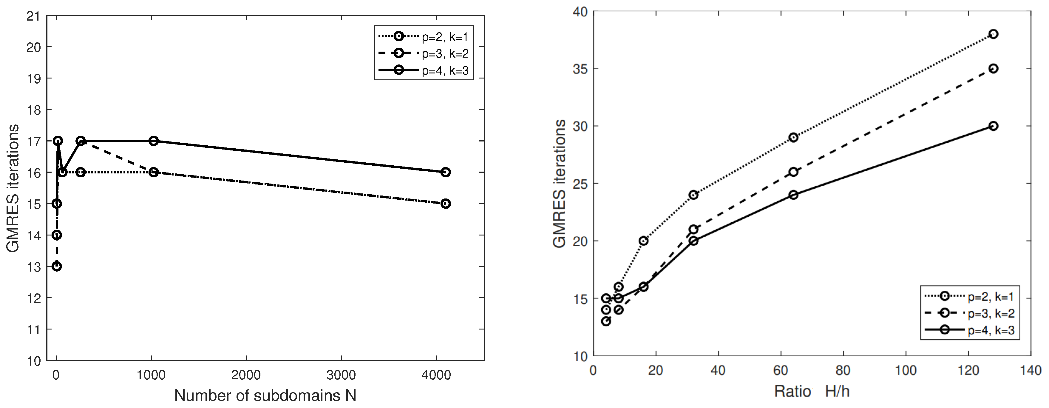
4.1. Two Spatial Dimension Tests: OAS Scalability in N and Optimality in H/h

We begin by analyzing the behavior of the condition numbers of the IGA collocation stiffness matrix based on GB-splines with respect to the mesh size h and the GB-spline degree p. The results for the unpreconditioned systems corresponding to various polynomial degrees p and the maximal regularity $k=p-1$, are presented on the 2D square domain in Table 1. These results indicate that the condition numbers of the collocation stiffness matrices exhibit an asymptotic growth rate of $h^{-2}$, highlighting the necessity of developing efficient iterative solvers for IGA collocation methods (IGA-C) based on GB-splines.

The GMRES iteration counts for the 1-level and 2-level overlapping additive Schwarz preconditioners (denoted as OAS (1) and OAS (2), respectively) are reported in

Table 2. GMRES iteration counts of unpreconditioned (NP) GMRES, OAS (1) and OAS (2) preconditioned GMRES in 2D unit square domain (for interpretation of the references to colour in this table legend, the reader is referred to the web version of this article).

$\mathit{p}=2,\mathit{k}=1,\mathit{r}=0$, 2D unit square domain
	$1/h$ = 8		$1/h$ = 16		$1/h$ = 32		$1/h$ = 64		$1/h$ = 128		$1/h$ = 256
NP	18		35		69		169		467		1198
N	OAS (1)	OAS (2)	OAS (1)	OAS (2)	OAS (1)	OAS (2)	OAS (1)	OAS (2)	OAS (1)	OAS (2)	OAS (1)	OAS (2)
$2\times 2$	12	14	15	16	19	20	26	24	33	29	45	38
$4\times 4$			18	17	25	20	34	23	45	29	62	37
$8\times 8$					30	16	43	21	62	26	85	34
$16\times 16$							55	16	81	20	122	27
$32\times 32$									109	16	209	19
$64\times 64$											324	15
$p=3,k=2,r=0$, 2D unit square domain
NP	22		42		84		213		601		1720
N	OAS (1)	OAS (2)	OAS (1)	OAS (2)	OAS (1)	OAS (2)	OAS (1)	OAS (2)	OAS (1)	OAS (2)	OAS (1)	OAS (2)
$2\times 2$	12	13	17	14	21	16	29	21	36	26	52	35
$4\times 4$			21	17	29	18	40	22	54	28	75	36
$8\times 8$					36	16	53	19	75	23	102	29
$16\times 16$							69	17	100	18	183	23
$32\times 32$									165	16	291	18
$64\times 64$											426	15
$p=4,k=3,r=0$, 2D unit square domain
NP	33		55		108		329		744		2447
N	OAS (1)	OAS (2)	OAS (1)	OAS (2)	OAS (1)	OAS (2)	OAS (1)	OAS (2)	OAS (1)	OAS (2)	OAS (1)	OAS (2)
$2\times 2$	12	15	15	15	19	16	25	20	32	24	43	28
$4\times 4$			17	17	24	17	33	19	44	24	60	30
$8\times 8$					28	16	41	19	58	23	82	28
$16\times 16$							53	17	75	19	114	25
$32\times 32$									98	17	192	19
$64\times 64$											304	16

for the two-dimensional parametric domain and in

Table 3. GMRES iteration counts of NP GMRES, OAS (1) and OAS (2) preconditioned GMRES in a quarter of an annulus (For interpretation of the references to colour in this table legend, the reader is referred to the web version of this article).

$\mathit{p}=2,\mathit{k}=1,\mathit{r}=0$, a quarter of an annulus
	$1/h$ = 8		$1/h$ = 16		$1/h$ = 32		$1/h$ = 64		$1/h$ = 128
NP	31		61		129		326		733
N	OAS (1)	OAS (2)	OAS (1)	OAS (2)	OAS (1)	OAS (2)	OAS (1)	OAS (2)	OAS (1)	OAS (2)
$2\times 2$	14	16	19	18	25	22	33	28	45	39
$4\times 4$			23	19	34	24	45	31	62	42
$8\times 8$					43	21	61	29	86	39
$16\times 16$							81	23	124	33
$32\times 32$									196	24
$p=3,k=2,r=0$, a quarter of an annulus
NP	38		69		168		424		909
N	OAS (1)	OAS (2)	OAS (1)	OAS (2)	OAS (1)	OAS (2)	OAS (1)	OAS (2)	OAS (1)	OAS (2)
$2\times 2$	16	15	21	18	28	22	37	28	51	37
$4\times 4$			29	22	39	27	54	34	73	44
$8\times 8$					52	26	76	33	109	42
$16\times 16$							104	30	179	37
$32\times 32$									244	31
$p=4,k=3,r=0$, a quarter of an annulus
NP	44		75		212		506		1226
N	OAS (1)	OAS (2)	OAS (1)	OAS (2)	OAS (1)	OAS (2)	OAS (1)	OAS (2)	OAS (1)	OAS (2)
$2\times 2$	14	17	18	17	24	20	32	24	42	31
$4\times 4$			21	19	32	22	43	27	60	35
$8\times 8$					41	21	59	27	83	34
$16\times 16$							78	22	115	31
$32\times 32$									191	23

for the deformed physical domain. These results are presented as a function of the number N of subdomains and the mesh parameter $1/h$ for various p with minimal overlap index $r=0$ and maximal regularity $k=p-1$. The findings indicate that the proposed OAS (2) preconditioners exhibit scalability, as GMRES iteration counts (in blue) remain bounded from above by a constant independent of N when following the diagonal trend in Table 2 and Table 3 (see also on the left of Figure 2). Furthermore, the results emphasize the critical role of the coarse problem in ensuring scalability; specifically, the OAS (1) preconditioner (lacking a coarse component) demonstrates increasing GMRES iteration counts as N grows along the diagonal entries of Table 2 and Table 3. In addition, numerical results also show that GMRES iteration counts (in red) increase less than linearly with the ratio $H/h$ (see also on the right of Figure 2).

4.2. OAS Robustness with Respect to 2D Domain Deformations

Now we numerically assess the performance of our proposed methods in the presence of domain deformations. In this test, we consider four progressively curved (boomerang-shaped) domains, labeled A, B, C, and D, as illustrated in Figure 3. All the domains for 2D deformation tests are discretized using the same mesh size $h=1/64$ and subdivided into $N=4\times 4$ subdomains. The numerical results in

Table 4. 2D domain deformation test: OAS robustness in the presence of domain deformations. GMRES iteration counts of NP GMRES, OAS (1) and OAS (2) preconditioned GMRES. Fixed $H/h=16$ ($1/h=64$ and $N=4\times 4$), $p=3$, $k=2$, and minimal overlap $r=0$.

2D Domain Deformation Test
Domain	NP	OAS (1)	OAS (2)
A	429	62	42
B	489	66	50
C	733	68	58
D	1268	74	75

demonstrate that OAS preconditioners show significantly lower sensitivity to domain deformations compared with the NP solver. Specifically, as the domain transitions from A to D, the GMRES iteration count for the unpreconditioned solver increases by a factor of 2.95, whereas for the OAS (2) preconditioner, the increase is limited to a factor of 1.78.

4.3. Three Spatial Dimensional (3D) Tests: OAS Scalability in N

The GMRES iteration counts of the unpreconditioned system, 1-level and 2-level OAS preconditioners for the 3D reference cubic domain are reported in

Table 5. OAS scalability in N on the 3D cubic domain: GMRES iteration counts of unpreconditioned (NP) GMRES, 1-level (OAS (1)) and 2-level (OAS (2)) preconditioned GMRES as a function of N with fixed $H/h=4,p=3,k=2$ and minimal overlap $r=0$.

N	NP	OAS (1)	OAS (2)
$2\times 2\times 2$	22	17	18
$3\times 3\times 3$	33	24	21
$4\times 4\times 4$	43	29	23
$5\times 5\times 5$	53	33	23
$6\times 6\times 6$	61	38	23

as a function of the number N of subdomains for fixed $H/h=4$, $p=3,k=2$ and minimal overlap $r=0$. These numerical results justify that only OAS (2) preconditioners are scalable, since GMRES iteration counts remain bounded from above by a constant independent of the number N of subdomains.

5. Conclusions

We have introduced overlapping additive Schwarz preconditioners for elliptic problems discretized with isogeometric collocation methods based on GB-splines and analyzed their performance through a selection of numerical tests in two and three spatial dimensions. In particular, our numerical results have shown the OAS (2) quasi-optimality with respect to the ratio $H/h$ and its scalability with respect to the number of subdomains N. We expect that our preconditioners can be robust with respect to the choice of collocation points [53] and with respect to the choice of coarse problem [28] and be extended to elliptic systems of elasticity on more complex single-patch domains as well as PDEs on multi-patch and trimmed computational geometries. p-robust OAS preconditioners will be the topic of future research, and optimal multilevel preconditioners for both IGA-G and IGA-C schemes based on GB-splines are additional future research directions.

References

1. Hughes, T.J.R.; Cottrell, J.A.; Bazilevs, Y. Isogeometric analysis: CAD, finite elements, NURBS, exact geometry, and mesh refinement. Comp. Meth. Appl. Mech. Engrg. 2005, 194, 4135–4195. [Google Scholar] [CrossRef]
2. Cottrell, J.A.; Hughes, T.J.R.; Bazilevs, Y. Isogeometric Analysis. Towards integration of CAD and FEA; Wiley: Hoboken, NJ, USA, 2009. [Google Scholar]
3. Bazilevs, Y.; da Veiga, L.B.; Cottrell, J.A.; Hughes, T.J.R.; Sangalli, G. Isogeometric analysis: Approximation, stability and error estimates for h-refined meshes. Math. Mod. Meth. Appl. Sci. 2006, 16, 1–60. [Google Scholar] [CrossRef]
4. da Veiga, L.B.; Buffa, A.; Sangalli, G.; Vazquez, R. Mathematical analysis of variational isogeometric methods. Acta Numer. 2014, 23, 157–287. [Google Scholar] [CrossRef]
5. Costantini, P.; Manni, C.; Pelosi, F.; Sampoli, M.L. Quasi-interpolation in isogeometric analysis based on generalized B-splines. Comput. Aided Geom. Design 2010, 27, 656–668. [Google Scholar] [CrossRef]
6. Kvasov, B.I.; Sattayatham, P. GB-splines of arbitrary order. J. Comp. Appl. Math. 1999, 104, 63–88. [Google Scholar]
7. Manni, C.; Pelosi, F.; Sampoli, M.L. Generalized B-splines as a tool in isogeometric analysis. Comput. Methods Appl. Mech. Engrg. 2011, 200, 867–881. [Google Scholar] [CrossRef]
8. Costantini, P.; Lyche, T.; Manni, C. On a class of weak Tchebycheff systems. Numer. Math. 2005, 101, 333–354. [Google Scholar] [CrossRef]
9. Lyche, T.; Manni, C.; Speleers, H. Tchebycheffian B-splines revisited: An introductory exposition. In Advanced Methods for Geometric Modeling and Numerical Simulation; Springer INdAM Series; Springer: Berlin/Heidelberg, Germany, 2019; Volume 35, pp. 179–216. [Google Scholar]
10. Mazure, M.-L. On a general new class of quasi-Chebyshevian splines. Numer. Algorithms 2011, 58, 399–438. [Google Scholar] [CrossRef]
11. Mazure, M.-L. How to build all Chebyshevian spline spaces good for Geometric Design. Numer. Math. 2011, 119, 517–556. [Google Scholar] [CrossRef]
12. Raval, K.; Manni, C.; Speleers, H. Tchebycheffian B-splines in isogeometric Galerkin methods. (English summary). Comput. Methods Appl. Mech. Engrg. 2023, 403, 115648. [Google Scholar] [CrossRef]
13. Buffa, A.; Sangalli, G.; Vàzquez, R. Isogeometric analysis in electromagnetics: B-spline approximation. Comput. Methods Appl. Mech. Engrg. 2010, 199, 1143–1152. [Google Scholar] [CrossRef]
14. Buffa, A.; Sangalli, G.; Vázquez, R. Isogeometric methods for computational electromagnetics: B-spline and T-spline discretizations. J. Comput. Phys. 2014, 257, 1291–1320. [Google Scholar] [CrossRef]
15. Manni, C.; Pelosi, F.; Sampoli, M.L. Isogeometric analysis in advection-diffusion problems: Tension splines approximation. J. Comput. Appl. Math. 2011, 236, 511–528. [Google Scholar] [CrossRef]
16. Manni, C.; Pelosi, F.; Speleers, H. Local hierarchical h-refinements in IgA based on generalized B-splines. In Mathematical Methods for Curves and Surfaces 2012; Floater, M., Ed.; Lecture Notes in Computer Science; Springer: Berlin/Heidelberg, Germany, 2014; Volume 8177, pp. 341–363. [Google Scholar]
17. Manni, C.; Roman, F.; Speleers, H. Generalized B-splines in isogeometric analysis. In Approximation Theory XV: San Antonio 2016; Springer Proceedings in Mathematics & Statistics; Springer: Berlin/Heidelberg, Germany, 2017; Volume 201, pp. 239–267. [Google Scholar]
18. Auricchio, F.; da Veiga, L.B.; Hughes, T.J.R.; Reali, A.; Sangalli, G. Isogeometric Collocation Methods. Math. Mod. Meth. Appl. Sci. 2010, 20, 2075–2107. [Google Scholar] [CrossRef]
19. Auricchio, F.; da Veiga, L.B.; Hughes, T.J.R.; Reali, A.; Sangalli, G. Isogeometric collocation for elastostatics and explicit dynamics. Comp. Meth. Appl. Mech. Engrg. 2012, 249–252, 2–14. [Google Scholar] [CrossRef]
20. Schillinger, D.; Evans, J.A.; Reali, A.; Scott, M.A.; Hughes, T.J.R. Isogeometric Collocation: Cost comparison with Galerkin methods and extension to adaptive hierarchical NURBS discretizations. Comp. Meth. Appl. Mech. Engrg. 2013, 267, 170–232. [Google Scholar] [CrossRef]
21. Auricchio, F.; da Veiga, L.B.; Kiendl, J.; Lovadina, C.; Reali, A. Locking-free isogeometric collocation methods for spatial Timoshenko rods. Comp. Meth. Appl. Mech. Engrg. 2013, 263, 113–126. [Google Scholar] [CrossRef]
22. da Veiga, L.B.; Lovadina, C.; Reali, A. Avoiding shear locking for the Timoshenko beam problem via isogeometric collocation methods. Comp. Meth. Appl. Mech. Engrg. 2012, 241–244, 8–51. [Google Scholar]
23. Gomez, H.; Reali, A.; Sangalli, G. Accurate, efficient, and (iso)geometrically flexible collocation methods for phase-field models. J. Comput. Phys. 2014, 262, 153–171. [Google Scholar] [CrossRef]
24. Cho, D. Overlapping Schwarz methods for isogeometric analysis based on generalized B-splines. Comput. Methods Appl. Mech. Engrg. 2020, 372, 113430. [Google Scholar] [CrossRef]
25. Trefethen, L.N.; Bau, D. Numerical Linear Algebra; SIAM: University City, PA, USA, 1996. [Google Scholar]
26. da Veiga, L.B.; Cho, D.; Pavarino, L.F.; Scacchi, S. Overlapping Schwarz methods for Isogeometric Analysis. SIAM J. Numer. Anal. 2012, 50, 1394–1416. [Google Scholar] [CrossRef]
27. da Veiga, L.B.; Cho, D.; Pavarino, L.F.; Scacchi, S. Isogeometric Schwarz preconditioners for linear elasticity systems. Comp. Meth. Appl. Mech. Engrg. 2013, 253, 439–454. [Google Scholar] [CrossRef]
28. da Veiga, L.B.; Cho, D.; Pavarino, L.F.; Scacchi, S. Overlapping Schwarz preconditioners for isogeometric collocation methods. Comp. Meth. Appl. Mech. Engrg. 2014, 278, 239–253. [Google Scholar] [CrossRef]
29. Cho, D. Isogeometric Schwarz Preconditioners with Generalized B-Splines for the Biharmonic Problem. Axioms 2023, 12, 452. [Google Scholar] [CrossRef]
30. Cho, D.; Pavarino, L.F.; Scacchi, S. Isogeometric Schwarz preconditioners for the biharmonic problem. Electron. Trans. Numer. Anal. 2018, 49, 81–102. [Google Scholar] [CrossRef]
31. Hofer, C. Analysis of discontinuous Galerkin dual-primal isogeometric tearing and interconnecting methods. Math. Mod. Meth. Appl. Sci. 2018, 28, 131–158. [Google Scholar] [CrossRef]
32. Hofer, C. Parallelization of continuous and discontinuous Galerkin dual-primal isogeometric tearing and interconnecting methods. Comput. Math. Appl. 2017, 74, 1607–1625. [Google Scholar] [CrossRef]
33. Hofer, C.; Langer, U. Dual-primal isogeometric tearing and interconnecting solvers for multipatch dG-IgA equations. Comput. Methods Appl. Mech. Eng. 2017, 316, 2–21. [Google Scholar] [CrossRef]
34. Hofer, C.; Langer, U.; Takacs, S. Inexact dual-primal isogeometric tearing and interconnecting methods. In International Conference on Domain Decomposition Methods; Springer: Cham, Switzerland, 2017; pp. 393–403. [Google Scholar]
35. Kleiss, S.K.; Pechstein, C.; Jüttler, B.; Tomar, S. IETI - Isogeometric Tearing and Interconnecting. Comp. Meth. Appl. Mech. Engrg. 2012, 247–248, 201–215. [Google Scholar] [CrossRef]
36. Pavarino, L.F.; Scacchi, S. Isogeometric block FETI-DP preconditioners for the Stokes and mixed linear elasticity systems. Comp. Meth. Appl. Mech. Engrg. 2016, 310, 694–710. [Google Scholar] [CrossRef]
37. da Veiga, L.B.; Cho, D.; Pavarino, L.F.; Scacchi, S. BDDC preconditioners for Isogeometric Analysis. Math. Mod. Meth. Appl. Sci. 2013, 23, 1099–1142. [Google Scholar] [CrossRef]
38. da Veiga, L.B.; Pavarino, L.F.; Scacchi, S.; Widlund, O.B.; Zampini, S. Isogeometric BDDC preconditioners with deluxe scaling. SIAM J. Sci. Comp. 2014, 36, A1118–A1139. [Google Scholar] [CrossRef]
39. da Veiga, L.B.; Pavarino, L.F.; Scacchi, S.; Widlund, O.B.; Zampini, S. Adaptive selection of primal constraints for isogeometric BDDC deluxe preconditioners. SIAM J. Sci. Comp. 2017, 39, A281–A302. [Google Scholar] [CrossRef]
40. Pavarino, L.F.; Scacchi, S.; Widlund, O.B.; Zampini, S. Isogeometric BDDC deluxe preconditioners for linear elasticity. Math. Models Methods Appl. Sci. 2018, 28, 1337–1370. [Google Scholar] [CrossRef]
41. Widlund, O.B.; Scacchi, S.; Pavarino, L.F. BDDC deluxe algorithms for two-dimensional H(curl) isogeometric analysis. SIAM J. Sci. Comput. 2022, 44, A2349–A2369. [Google Scholar] [CrossRef]
42. Buffa, A.; Harbrecht, H.; Kunoth, A.; Sangalli, G. BPX-preconditioning for isogeometric analysis. Comp. Meth. Appl. Mech. Engrg. 2013, 265, 63–70. [Google Scholar] [CrossRef]
43. Donatelli, M.; Garoni, C.; Manni, C.; Serra-Capizzano, S.; Speleers, H. Robust and optimal multi-iterative techniques for IgA Galerkin linear systems. Comp. Meth. Appl. Mech. Engrg. 2015, 284, 230–264. [Google Scholar] [CrossRef]
44. Gahalaut, K.; Kraus, J.; Tomar, S. Multigrid Methods for Isogeometric Discretization. Comp. Meth. Appl. Mech. Engrg. 2013, 253, 413–425. [Google Scholar] [CrossRef]
45. Gahalaut, K.P.S.; Tomar, S.K.; Kraus, J.K. Algebraic multilevel preconditioning in isogeometric analysis: Construction and numerical studies. Comp. Meth. Appl. Mech. Engrg. 2013, 266, 40–56. [Google Scholar] [CrossRef]
46. Hofreither, C.; Takacs, S. Robust multigrid for isogeometric analysis based on stable splittings of spline spaces. SIAM J. Numer. Anal. 2017, 55, 2004. [Google Scholar] [CrossRef]
47. Takacs, S. Robust approximation error estimates and multigrid solvers for isogeometric multi-patch discretizations. Math. Models Methods Appl. Sci. 2018, 28, 1899–1928. [Google Scholar] [CrossRef]
48. Cho, D. Optimal multilevel preconditioners for isogeometric collocation methods. Math. Comput. Simul. 2020, 168, 76–89. [Google Scholar] [CrossRef]
49. Cho, D.; Pavarino, L.F.; Scacchi, S. Overlapping additive Schwarz preconditioners for isogeometric collocation discretizations of linear elasticity. Comput. Math. Appl. 2021, 93, 66–77. [Google Scholar] [CrossRef]
50. de Boor, C. A Practical Guide to Splines; Springer: Berlin/Heidelberg, Germany, 2001. [Google Scholar]
51. Lyche, L. A recurrence relation for Chebyshevian B-splines. Constr. Approx. 1985, 1, 155–173. [Google Scholar] [CrossRef]
52. Wang, G.; Fang, M. Unified and extended form of three types of splines. J. Comp. Appl. Math. 2008, 216, 498–508. [Google Scholar] [CrossRef]
53. Manni, C.; Reali, A.; Speleers, H. Isogeometric collocation methods with generalized B-splines. Comput. Math. Appl. 2015, 70, 1659–1675. [Google Scholar] [CrossRef]
54. Vázquez, R. A new design for the implementation of isogeometric analysis in Octave and Matlab: GeoPDEs 3.0. Comput. Math. Appl. 2016, 72, 523–554. [Google Scholar] [CrossRef]
Figure 1. Spectrum of the unpreconditioned operator (first row), OAS (1) (second row) and OAS (2) (third row) preconditioned operators on 2D square domain, N = 16 (first column), N = 64 (second column), N = 144 (third column), H / h = 4 , p = 3 , k = 2 , r = 0 (see, e.g., [25] for a condition on a fast GMRES convergence).
Axioms 14 00397 g001
Figure 2. GMRES iteration counts (in blue) in Table 2 for increasing N with fixed H / h = 4 (left). GMRES iteration counts (in red) in Table 2 for increasing H / h with fixed N = 2 × 2 (right). OAS (2) preconditioners with coarse spaces, minimal overlap r = 0 , ( p = 2 , k = 1 ), ( p = 3 , k = 2 ) and ( p = 4 , k = 3 ) on the unit square domain.
Axioms 14 00397 g002
Figure 3. Domains for the 2D domain deformation test.
Axioms 14 00397 g003