Abstract
Competing patterns are compound patterns that compete to be the first to occur a pattern-specific number of times, known as a stopping rule. In this paper, we study a higher-order Markovian dependent Bernoulli trials model with competing patterns. The waiting time distribution refers to the distribution of the number of trials required until the stopping rule is met. Based on a finite Markov chain, a hierarchical algorithm is proposed to derive the conditional probability generating function (pgf) of the waiting time of the competing patterns model. By applying the law of total expectation, the final pgf is then obtained. Using examples, we further demonstrate that the proposed algorithm is an effective and easy-to-implement tool.
MSC:
60-08; 60J10; 90-10
1. Introduction and Literature Review
The waiting time distribution for a sequence of trials refers to the distribution of the number of trials required until a specific stopping rule is satisfied. A series of identical trials is referred to as a “run”, while a general sequence is called a “pattern”. The waiting times of a sequence of trials have been extensively studied with different stopping rules. Most of these studies employ combinatorial analysis, assuming a sequence of independent and identically distributed (i.i.d.) trials, each of which ends in two or more outcomes.
The most basic model dates to i.i.d. Bernoulli trials (each resulting in either a success “1” or a failure “0”), where the stopping rule is the occurrence of the first success (“1”). Here, the waiting time is a geometrically distributed random variable (r.v.). When the stopping rule is extended to the k-th success, the waiting time is Negative Binomial (NB) r.v. More complex stopping rules include specific sequences, combinations of multiple stopping rules, multi-state trials, and Markovian models (with dependent trials).
The waiting time distributions of runs and patterns, such as geometric, geometric of order k, negative binomial, and sooner and later, have been successfully applied in numerous areas of statistics and applied probability. In recent decades, the theory of waiting time distributions has become an indispensable tool for studying various applications, including DNA sequence homology (Schwager [1], Karwe and Naus [2,3]), epidemiology (Kulldorff [4]), and system reliability (Aki [5], Aki and Hirano [6], Chang and Huang [7]). We will now present some specific examples.
Studying the distribution of patterns assists in DNA sequence analysis by modeling the occurrence of specific motifs, repeats, or base combinations. Each nucleotide position is treated as a Bernoulli trial, allowing researchers to detect biologically significant patterns such as transcription factor binding sites, identify mutation hotspots, and study codon usage bias. It also aids in evaluating the statistical significance of sequence alignments and testing whether observed patterns are random or functionally important, providing insights into DNA structure, function, and evolution. In this regard, Kulldorff [4] investigated the occurrences of sudden infant death syndrome or birth defects using the Bernoulli model. In psychology, Schwager [1] explored the concept of “success breeds success” or “failure breeds failure” which is applied in achievement testing, animal learning studies, athletic competition, and study performance improvement. He further demonstrated that the behavior of groups of people forming lines and other structures can be modeled as a Markov-dependent sequence of trials in which some characteristic, such as the sex of the individual, is taken as a trial outcome. Dafnis [8] demonstrated a practical application for the waiting time distribution of binary trials in the topic of meteorology and agriculture, by considering the cultivation of raisins. The harvesting of certain varieties of raisins in Greece must occur between August and September. For the harvesting, a period of at least four consecutive dry days is required. Before this period begins, a period of at least two consecutive rainy days is required to water the raisins. Dafnis [8] used “0” to denote the occurrence of a rainy day, and “1” to denote the occurrence of a dry one. The probabilities of “0” and “1” were estimated using previous years’ statistics.
In the field of agriculture, the concept of r-weak runs distribution was applied to identify the rate of development of crops (which recognizes that plant development will occur only when the temperature exceeds a specific base temperature for a certain number of days), and to investigate the impact of critical factors on honeydew honey production (Dafnis et al. [9], Dafnis et al. [10]). Drawing our attention to reliability studies, we mention the consecutive k-out-of-n systems. In these systems, each component is either working or failed, and the overall system functions only when at least k consecutive components are working within the total n components in the sequence. Dafnis et al. [11] studied the k-out-of-n system that fails if and only if a string of k non-functioning components is interrupted by a string of at most r consecutive functioning ones. They showed that there are different patterns of appearance that can cause a system failure. In the financial field, Dafnis and Marki [12] showed how the concept of r-weak runs can be adapted by financial advisors and technical analysts for the determination of a personalized and effective investing strategy with controlled risk.
For the literature review, we date back to Feller [13], who studied the probability generating function (pgf) for the waiting time distribution of a sequence of i.i.d Bernoulli trials where the stopping condition is the first occurrence of a series of k consecutive successes. Philippou et al. [14] extended Feller [13] by studying a geometric distribution of order k, defined as the waiting time distribution until k consecutive successes occur. Aki [5] generalized the model to geometric, NB, Poisson, logarithmic series, and binomial distributions of order k with dependencies. Philippou and Makri [15] studied the binomial distribution of order k in a finite number of Bernoulli trials. Philippou [16] studied multi-state trials, and Ling [17] extended the k-th ordered geometric model with parameter p to -order with parameter ; the exact distributions and the pgfs were further derived for some special cases of . Shmueli and Cohen [18] used recursive formulas to compute the exact probability functions of a model with switching rules. Koutras and Eryilmaz [19] considered a compound geometric distribution of order k determined by another random process, such as Poisson or binomial.
The above literature assumes that the experiment ends after the first k consecutive successes. A more general stopping rule is to stop the experiment with the first occurrence of a particular sequence of i.i.d. Bernoulli experiments, known as a pattern. A pattern has a specific sequence and may include different symbols. In this context, Blom and Thorburn [20] analyzed the waiting time distribution until a k-digit sequence is obtained or, more generally, until one of several k-digit sequences is obtained. For the latter case, the mean waiting time was also derived. Ebneshahrashoob and Sobel [21] studied a generalized pgf, means and variances for the waiting time until obtaining a sequence of s successes or a sequence of r failures, whichever comes sooner. Huang [22] introduced a generalized stopping -rule as the occurrence of consecutive failures followed by consecutive successes. Dafnis et al. [8], Makri [23] and Kumar and Upadhye [24] considered different types of -rules. Zhao et al. [25], Kong [26] and Chadjiconstantinidis and Eryilmaz [27] studied the distributions of -runs of multi-state trials.
To date, we focused on the distribution of the first instance of a pattern, or the -type model. We next reviewed the literature dealing with the distribution for the r-th occurrence of a pattern. Aki [28] investigated the waiting time distribution until the r-th occurrence of a pattern in a sequence of i.i.d. Bernoulli trials. Koutras [29] derived several moments of the waiting time for the non-overlapping appearance of a pair of successes separated by at most k − 2 failures (). Robin and Daudin [30] obtained the distribution of distances between the two successive occurrences of a specific pattern, as well as between the n-th and the -th occurrences. Aki and Hirano [31] further explored a two-dimensional pattern model.
Focusing on models under the assumption of Markov dependency, Hirano and Aki [32] studied the distribution of the number of success runs of length k until the n-th trial in a two-state dependent Markov chain. Fu and Koutras [33] presented an approach for the distribution theory of runs based on a finite Markov chain embedding technique that covers identical and nonidentical Bernoulli trials. In addition, the exact distribution of the waiting time for the m-th occurrence of a specific run, and the distribution of the number of at least k successes were derived. The number of failures, successes, and the first consecutive k successes were studied in Aki and Hirano [31]. Using non-overlapping counting, Fu [34] studied the multi-state trials model. Koutras [35] developed a general technique for the waiting time distribution in a two-state dependent Markov chain. Antzoulakos [36] introduced a variation of the finite Markov chain embedding method to derive the pgf until the r-th occurrence of a pattern, considering both non-overlapping and overlapping cases. Fisher and Cui [37] introduced a mathematical framework for determining the expected time for a specific pattern to emerge in higher-order Markov chains, both with and without a predefined starting sequence. This approach was extended to the calculation of the first occurrence of any pattern from a collection, along with the probability that each individual pattern is the first to appear. Chang et al. [38] studied the dual relationship between the probability of the number of patterns and the probability of the waiting time in a sequence of multi-state trials.
We next focused on models with stopping rules that involve a few simple patterns, known as the compound patterns rule, where the stopping rule is triggered by the first appearance of one of the patterns. Applying pgf techniques, Fu and Chang [39] and Han and Hirano [40] investigated multi-state trial models with compound patterns for both i.i.d. trials and first-order Markov-dependent trials. For the r-th order Markov-dependent chain, Fu and Lou [41] examined the waiting time distributions of the first occurrence of simple and compound patterns in the sequences of Bernoulli trials. Wu [42] applied a finite Markov chain embedding technique to analyze the conditional waiting time distributions. Using a matrix form, Aston and Martin [43] presented an algorithm that computes the distribution of the waiting time until the m-th occurrence of a compound pattern. For an excellent summary of various calculation methods, we refer readers to the comprehensive book by Fu and Lou [44] and Balakrishnan and Koutras [45].
Our research addresses models with a competing pattern stopping rule. Here, the experiment ends when a simple or compound pattern occurs a specific number of times (note that the compound pattern rule is a special case, where the experiment ends after the first occurrence). For a real-life example, consider again the cultivation of raisins (Dafnis [8]). To obtain raisins of fine quality, grapes need successions of short rainy and dry periods. Thus, an agriculturalist cares about the frequent occurrence of patterns with at most 2 consecutive rainy days followed by at most 2 consecutive dry days. Agriculturalists further claim that the occurrence of at least five such patterns in the three months has a significant effect on the quality of raisins.
Another real-life example is taken from Dafnis et al. [9]. They studied the effect of the number of cold days on the life cycle of Marchalina hellenica. They showed that the number of cold periods (each of which is a run of k consecutive cold days) is a more critical factor to the completion time of the insect’s biological cycle than the total number of cold days.
For models with competing patterns, Aston and Martin [43] investigated the waiting time distribution for competing patterns in m-th order dependent multi-state Markov trials. They analyzed several compound patterns, each associated with a specific required number of occurrences. Martin and Aston [3] introduced the generalized later patterns model, in which all patterns must appear multiple times. We also mention the closely related sooner and later models. Sooner waiting time distribution captures the number of trials required for the first occurrence of one of two competing patterns, and conversely, later waiting time distribution refers to the number of trials required for both patterns to occur (see, e.g., Han and Hirano [40], Balakrishnan and Koutras [45]).
For other related models dealing with waiting time distributions under the Markovian assumption, we mention the hidden Markov processes (Aston and Martin [46]), in which the states are not directly observable, or the sparse Markov process, in which the transition probability matrix includes many zero or near-zero entries (see, e.g., Martin [47,48]). Dafnis [10] studied the model with independent but not necessarily identically distributed trials. Michael [49] and Vaggelatou [50] presented a framework for a continuous time Markov chain. Dafnis et al. [9] introduced the r-weak run of length at least k in a sequence of binary trials. Their model was extended to include minimum and maximum constraints (Dafnis and Makri [12]). In a series of papers, Makri ([51,52]) investigated a sequence of binary trials with a specific length threshold.
Our paper contributes to this study by deriving simple and closed-form expressions for the pgf of waiting time distributions associated with higher-order Markovian-dependent Bernoulli trials with competing patterns. To the best of our knowledge, the studies presented to date are based on Markov chain-embedding techniques, where the state space is large, leading to a complicated transition probabilities matrix, high computational complexity and, thus, it is difficult to implement. The suggested algorithm is based on a hierarchical approach and includes three steps. In the first step, the framework is designed by including the state space, stopping rules, and steady-state probabilities. The second step determines all the paths that terminate the experiment; each such path is divided into sub-paths (components) where the total pgf is the product of the pgfs of these sub-paths. The last step derives the pgf of each sub-path by considering whether the path is longer or shorter than the number of trials of the longest pattern. The final pgf is obtained by applying the law of total expectation.
The rest of the paper is organized as follows. Section 2 introduces the definitions and preliminaries to be used. Using a hierarchical approach, Section 3 provides a mathematical description of the model and derives the pgf of the waiting time; this derivation is demonstrated by an example. A summarizing algorithm and additional examples are provided in Section 4. Finally, Section 5 concludes the paper and suggests some future directions. Following the convention, we indicate vectors by bold letters, and matrices by blackboard bold letters. We let be the indicator of an event be the column vector of all ones, and be the identity matrix, all of the appropriate dimensions. We use to denote the number of elements in a set Summarizing our abbreviations, we use pgf(s) for probability generating function(s), i.i.d r.v.(s) for independent and identical distributed random variable(s).
2. Definitions and Preliminaries
We use the terminology of Fo and Lou [41] and Aston and Martin [43].
Bernoulli trial. Consider a sequence of Bernoulli trials where each trial (symbol) has two possible outcomes, success and failure (0 and 1, respectively) with and Let be the state space of an individual result i.e.,
A simple pattern. A simple pattern is a specific sequence of k trials (symbols), from , i.e., The waiting time random variable of a simple pattern, is defined as
i.e., … counts the number of trials until the first occurrence of pattern . In the following, we assume that we start at .
A compound pattern is the union of l simple patterns. We use to denote the occurrence of either pattern or pattern . Accordingly, the waiting time is defined as
Note that
A (discrete) Markov chain. A discrete-time Markov chain is a sequence of random variables , … with the Markov property, namely that the probability of moving to the next state only depends on the present state and not on the previous states:
if both conditional probabilities are well defined, that is, if The possible values of form a countable set , called the state space of the chain. Time-homogeneous Markov chains are processes where for all t, i.e., the probability of the transition is independent of t (for more details, see Feller [13] and Hirano and Aki [32]).
An r-th order Markov chain. Let be a sequence of irreducible, aperiodic, and homogeneous r-th order Markov-dependent m-state random variables (trials) defined on the state space (when we have a Bernoulli trial). For the set of all possible r tuples ( combinations) is given by
The r-order transition probabilities of the Markov chain are defined by:
which is independent of t. The steady-state probability vector exists and satisfies where is the transition probability matrix.
In this work, we consider Bernoulli trials with .
Result 1. Let be an r-th order Markov chain. Fu and Lou [41] showed that there exists an embedded finite Markov chain defined on a state space where is the absorbing state. Accordingly, the transition probability matrix has the form
(Note i.e., the sum of the probabilities in each row of is equal to 1). The waiting time of a pattern (simple or compound) has a general geometric distribution
( is the initial distribution, and is known as the essential transition probability matrix). For more details, see Lemma 3.1, Theorems 3.1–4.2 of Fu and Lou [41].
Competing patterns. Let , be the set of c compound patterns. Let denote the number of occurrences of the compound pattern that terminates the experiment. The patterns are called competing patterns. We assume that no two competing compound patterns are identical.
Let be the event that, by time n, the compound pattern has occurred times. Then, the is the waiting time probability function of the competing patterns.
We further note that two distinct methods of counting patterns are considered in the literature (Inoue and Aki [53]). (1). Non-overlapping counting. In this case, when a pattern occurs, the counting restarts from that point, and any partially completed pattern cannot be finished. (2). Overlapping counting. In this case, partially completed patterns can be finished at any time, regardless of whether another pattern has been completed after the partially completed pattern starts but before it is completed.
Furthermore, we have two more definitions (Aston and Martin [43]): Ending blocks of a simple pattern are sub-patterns of the form , where . Ending blocks always start at the beginning of a simple pattern but end at any point before its last symbol. Finishing blocks of the simple pattern are sub-patterns of the form , where Finishing blocks may start at any point but always end with the last symbol. The finishing blocks of a compound pattern or competing patterns are formed by taking the union of the finishing blocks of their respective components.
Result 2. Consider the competing patterns . Aston and Martin [43] showed that the waiting time distribution for competing compound patterns has a geometric form. Specifically, the competing pattern experiment ends with compound pattern occurred times if and only if the Markov chain is absorbed in the corresponding absorbing state. Therefore, the probability function of the waiting time is given by
where is the initial probability vector of is the transition probability matrix, and is a column vector with 1’s in the position corresponding to the absorbing states and 0’s elsewhere (see Section 3.2 of Aston and Martin [43]).
Probability Generating Function
The probability generating functions (pgf) is a useful technique for computing distributions (see, e.g., Feller [13], chapter XI). As a short background, for a non-negative discrete random variable Y, the pgf is defined as
for all for which the sum converges. The pgf is then a power series and obeys all the rules obeyed by power series with non-negative coefficients. The probabilities are the coefficients of the power series, and may be recovered through series expansion or by taking derivatives of G with respect to z.
Pgfs are especially useful for computing the distributions of sums of random variables, as well as moments and factorial moments. We note that, for independent random variables , the pgf of is given by
Along with the uniqueness of the pgf, it is helpful to determine the sampling distribution of interest.
3. Competing Patterns in High-Order Markov-Dependent Bernoulli Trials
The derivation of the probability generating function includes three steps. In the first step, we build the mathematical framework, the experiment design and settings of the experiment. The second step determines the paths that terminate the experiment. Applying tools from probability theory and Markov chain, the third step derives the pgf function of the number of trials (waiting time) for each path. All steps are illustrated by a continuous example.
3.1. Step 1. Experimental Design and Settings
Consider the r-th order Markov-dependent Bernoulli trials on the state space (with combinations)
The r-th order transition probabilities are given by:
independent of t.
Clearly, for all In a matrix form, let be the square matrix with elements given by
Associated with the sequence are the initial probabilities
(Note that and the vector satisfies the system of equations Let be a compound pattern that includes simple patterns, each of which has size We assume that Let denote the number of non-overlapping occurrences of needed for the termination of the experiment, and let Let be the set of competing patterns, and let denote the waiting time random variable (number of trials) until the experiment terminates given the steady-state environment. We assume non-overlapping counting.
Example 1.
Our base case considers second-order Markov-dependent Bernoulli trials, i.e., and The transition probabilities are:
In a matrix form
(Note that ). Here, the steady-state probability vector satisfying is given by:
We assume two competing patterns (): with (), and with (). That is, the experiment terminates if either three occurrences of two consecutive (failures) or two occurrences of three consecutive 1s (successes) are observed.
3.2. Step 2. Stopping Paths
We start by applying a higher hierarchical point of view, focusing on paths of patterns rather than on individual trials. Clearly, several paths can terminate the experiment. Let be the set of paths that terminate the experiment due to Concretely, the set includes all paths that have the following structure: the pattern appears times in total, in which its last -th occurrence (that terminates the experiment) is the last component of the path; other occurrences of appear no more than times each. Assume that there are such paths (i.e., ). Denote these paths by so that In the following, each path will be referred to as a “stopping vector”. Let be the set of all stopping vectors that terminate the experiment.
Corollary 1.
It is easy to verify the following:
- (i)
- The number of competing patterns in each path satisfies:
- (ii)
- The number of paths in the set is given by (combinatorial considerations):(Note that the summing is over all patterns excluding ).
- (iii)
- Since including distinct patterns, we have:
Example 2.
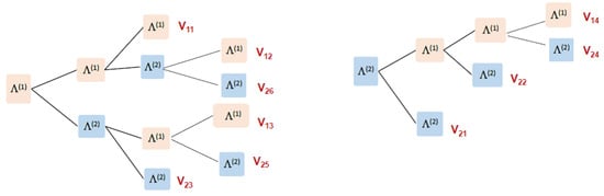
We have with , and with thus, the experiment terminates if either three occurrences of two consecutive or two occurrences of three consecutive 1s appear. Let and be the sets of paths that terminate the experiment due to and respectively. Figure 1 illustrates the sequence (path) of possible patterns that terminate the experiment (denoted by ; see the red labels). We observe that contains four possible paths () and contains six possible paths (). In summary, there are a total of 10 possible paths (stopping vectors) that end the experiment.
Figure 1.
The possible paths of and that terminate the experiment.
Applying Corollary 1(i), each such stopping vector includes at least two patterns (due to ) and no more than four patterns (). Applying Corollary 1(ii), the sets and include and stopping vectors, respectively. By Corollary 1(ii), and are given by:
and vectors (see also Figure 1),
Remark 1.
Note that Figure 1 presents only the paths of competing patterns; intermediate trials that do not lead to a pattern are not presented.
We then derive the probability-generating function of the waiting time until the experiment terminates.
3.3. Step 3. The Waiting Time Distribution
Let denote the waiting time until the experiment terminates with its pgf. Applying the law of total expectation and noting that are disjoint vectors (each vector refers to a different path) leads to:
( is the indicator function). Each stopping vector is composed of a numbered sequence of consecutive patterns , e.g., Let be the number of trials from pattern until the occurrence of the next pattern Accordingly, for we let be the number of trials until the first pattern occurs, given initial state . Let be the waiting time due to path It is easy to verify that:
Assume that the pattern − occurs (for we assume an initial state Let be the pgf of i.e., the pgf of the number of trails from − until ,
Note that, due to the Markovian property, the non-overlapping feature, and assuming the waiting time is independent of Therefore, we have:
We further note that the function is homogeneous, depends only on the patterns (and is independent of k). Thus, for simplicity, and without losing generality, we will use to denote the waiting time between two consecutive patterns and given that the pattern occurs ( permutations) and, respectively, to be the pgf of Accordingly, we let be the pgf of the number of trials until the first appearance of given the initial state
Example 3.
Two competing patterns yield four pgfs that differ in their starting and ending patterns, namely , and In addition, we have two functions, and corresponding to the first occurrence of and respectively. The total pgf is the sum of the ten distinct stopping vectors in each of which consists of the multiplication of the corresponding pgf along the path Specifically, we have:
Our next step is to derive the probability-generating functions and for Recall that is the longest length of pattern in and let Our aim is to apply the law of total expectation as a function of the number of trials between two consecutive patterns (or until the first pattern), distinguishing whether the number is less or equal to b or not. Thus, we use the decomposition:
In the left-hand side of (16), where the number of trials is no more than b, the derivation is relatively simpler and consists of a finite number of paths. Conversely, the derivation of the right-hand side of (16), where more than b trials are possible, is more challenging. We start with the relatively simpler derivation, and
3.3.1. The Functions
We first highlight the main difference between and The function refers to the first b trials; here, we use the steady-state probability vector , multiplied by the remaining probabilities. In contrast, the function assumes that the occurs, and continues with the multiplication of at most b transition probabilities leading to .
To derive recall that Let be the probability of hitting by no more than b trials (and no other patterns are hit). Let be the set of sequences of u trials in which appears in the last trials and no other pattern is hit; recall that Denote by the ergodic probability of . Clearly, when includes only the one pattern with probability When , there may be few paths in each denoted by starts with (with probability ), multiplying by a path of transition probabilities that leads to the ending pattern Thus, the ergodic probability distribution has the form of:
The function is then,
To derive we assume that, at time , the state includes the last r trials of and consider the set Each path in the set adds a component to with the product of the corresponding transition probabilities multiplied by . We next demonstrate (18) using our example.
Example 4.
Here, and . To derive we consider the pattern with Here, or When we have and when we have and Next, we derive Here, thus, with the only path and Summarizing, we obtain:
Next, we derive We assume that, at time , the state is the last r trial of (i.e., for we assume and for we assume . The function is constructed by a path of at most three multiplications of transition probabilities (multiplied by the corresponding power of z) that lead to . Here, we obtain:
i.e., when assuming (with the paths 00 and 100 (w.p. and respectively) lead to and the path 111 (w.p. ) leads to Similarly, when assuming (with ), the paths 00 and 100 (w.p. and respectively) lead to and the path 111 (w.p. ) leads to
3.3.2. The Functions
Let us consider the first b trials We group all that contain the pattern into the set Define the state to be the absorbing state due to pattern i.e., groups all states in Denote the absorbing vector by The set groups all states that do not include a pattern. Note that every state in has pattern of length b. Let be the transition probability matrix among the states in In addition, let be the absorbing probability vector at state and define the absorbing matrix We construct the embedded homogeneous Markov chain on the state space The transition probability matrix has the block form
where
Note that . The initial probability of is given by:
Since the initial probability for starts with the corresponding steady-state probability multiplying by the transition probabilities along the path . To complete the derivation, we need to define two row probability vectors of order , and Both vectors represent the probability of entering into the states in after b trials with no competing patterns; the difference arises from their initial conditions. The vector assumes an initial state in (not including a pattern), and calculates the probability of entering at time ; here, we use the steady-state probability vector of order r, and a multiplication of successive transition probabilities. The vector assumes an initial pattern and derives the probability of entering afterward; here, we use a multiplication of b successive transition probabilities.
Proposition 1.
The functions and have the general form of:
Proof.
The derivation of and is composed of three parts. In the first part, the experiment enters a state within the set after b trials where no hitting occurs. Thus, we multiply and by respectively. The second part is the pgf of the number of trials to stay in the set until absorption. Here, following Fu and Lou [41], we have the term From that point, the third part is the probability of hitting in the next trial, with pgf □
Remark 2.
An easy way to derive the vectors and is as follows. Construct the transition probability matrices and The matrix present the probability of each state in , given an initial r-state trial. The vectors can be extracted from by taking the corresponding row to the r ending block of and the corresponding columns with the appropriate eliminations.
Example 5.

Since we have and Here, and We construct the embedded homogeneous Markov chain on the state space
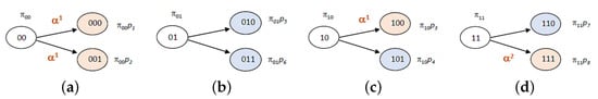
To clarify, Figure 2a–d illustrate the states and probabilities of states marked by light red, including a pattern and, thus, are marked by or
Figure 2.
The states and probabilities of , given (a)
, (b) , (c) , (d) .
Summarizing, the initial distribution probability of is given by (note that ):
The transition probability matrix has the form and is given by (Table 1):
Table 1.
The probability transition matrix of .
To complete our derivation, we need to derive the vectors and Note that the vector is the sub-vector of with the corresponding vectors in i.e.,
(Note that, since is a competing pattern, the vector considers only the two-state trials {01,10,11}). In order to derive and we apply Remark 2. Here, the matrices and are given by (Table 2):
Table 2.
The probability transition matrix of .
And thus, is given by:
The probability vectors and to be at state in three trials without hitting, starting from and respectively, are highlighted by the red boxes; see the first and last rows in Table 3. Here, we obtain
Table 3.
The probability transition matrix of .
(Note that is also obtained by taking the columns corresponding to in the product ). Summarizing all, we have:
Substituting (28) in (15) completes the derivation of G(z).
4. Algorithm and Examples
To summarize, we next present an algorithm with the main key steps; a detailed pseudocode is provided in Appendix A. The algorithm is then demonstrated by two additional examples.
4.1. The Algorithm
Step 1. Inputs and initialization
- The parameter the space state the -square transition matrix .
- The competing patterns and their appearances:
- Calculate the steady-state probability vector satisfying
Step 2. Embedded Markov chain
- Set
- Build the state space define the absorbing states
Step 3. Probability generating function
- Calculate the vector and the matrices and Derive (the matrix can be helpful with the appropriate eliminations).
- Apply (G14) to obtain and
4.2. Example 2
Our next example is inspired by ReasonLabs. ReasonLabs Ltd. is a global pioneer in cybersecurity detection and prevention powered by machine learning (https://reasonlabs.com) (accessed on 10 January 2025). The Israeli team (called the Performance team) is responsible for projects marketing via a website. Their marketing occurs in several stages, in which a customer is expected to enter the website and choose the service that suits their needs. Basic services are free, while premium services are purchased. Usually, a customer (buyer) visits the website a few times for various projects. The Performance team’s purpose is to track customer acquisition and identify buyer patterns, especially those who are willing to purchase the premium service. To achieve this, they use Bernoulli trials, where each outcome represents a customer choice. The result ‘1’ represents purchasing a premium service, and ‘0’ represents choosing a free service. Two stopping rules are proposed to detect the customer behavior:
(1) Two consecutive purchases (1s) occurring twice (not necessarily consecutively). Here, we also allow at most one free service (‘0’) between them. This customer is considered the most serious buyer to track.
(2) Two consecutive free enters (0s) occurring twice (not necessarily consecutively). This customer is considered a less serious customer who can be ignored.
The above rules (1) and (2) can be modeled as a waiting time problem of competing patterns. We next demonstrate the algorithm on Example 2.
Step 1. Consider second-order Markov-dependent Bernoulli trials, with transition probabilities given in (4)–(6). Here, we have two competing patterns, with (associated with Rule 1), and with (associated with Rule 2). Thus, the experiment terminates when one of the following rules occurs:
- (i)
- Two occurrences of the set of patterns i.e., either 101 occurs twice, or 11 occurs twice, or 101 and then or vice versa, all occurrences are not necessarily consecutive.
- (ii)
- Two (not necessarily consecutive) occurrences of two consecutive .
Example of the sequences are, e.g., 010100011, 11100101 (Rule (i)), and 0100101100, 01011000100 (Rule (ii)).
Step 2. Accordingly, we have two sets and corresponding to and respectively. Figure 3 demonstrates the paths of possible patterns that terminate the experiment. We observe that and include three possible paths each (), and (). Thus, we have six possible paths in total (stopping vectors) that terminate the experiment.
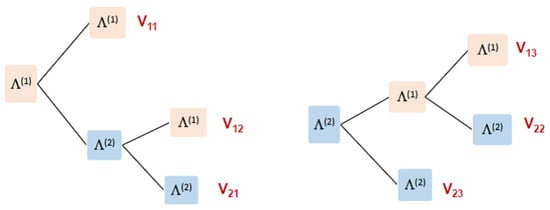
Figure 3.
The possible paths of or that terminate the experiment.
Corollary 1(i) yields that each such stopping vector includes at least two patterns and no more than three patterns (). By Corollary 1(ii), and are given by:
and vectors. Specifically, the stopping vectors are (see Figure 3):
Since we have two competing patterns, and there are four pgfs, in addition to (the pgf of the first occurrence of and respectively). Furthermore, the pattern includes two simple patterns Thus, to distinguish between them, we mark by the sign “′”, and refer to by no sign. Hence, we need to derive and The final pgf will be (to be shorter, the parameter z is omitted):
Here, the longest pattern is , so and }. We obtain , and Thus, and the vectors (in fact, scalars) are and (see the red rectangles in Table 4). The absorbing vectors (scalar) are and Also, note that the transition matrix is and = This result is due to the fact that, when we have the sequence either trial 0 or 1 immediately yields a hit. The immediate conclusion is that the waiting time for a single hit is no more than four trials.
Table 4.
The probability transition matrix of .
Step 3. We next derive and the pgfs
The function is constructed by a path of at most three multiplications of transition probabilities:
Summarizing everything, we have:
To add real data, the ReasonLabs Performance team further conducted an estimation of daily user-choice probabilities for free vs. premium services, focusing on the two most recent days of user activity,
The above probabilities show that those who switch from free to premium have a 50% chance of reverting and a 50% chance of continuing with premium, while in the opposite case, i.e., those who switch from premium to free have a 60% likelihood of switching back to premium. We also see that 80% of users that chose premium twice will stay premium, and 70% of free users will try premium. These probabilities suggest that users are likely to move toward premium.
Based on these estimates, the probability vector and the pgf of the waiting times are given by:
with an average number of trials of 5.805 and a variance of 3.197. The information that it takes approximately 6 visits (with a minimum of 4 and a maximum of 12 visits) to classify a customer may help in the optimization of resource allocation and preventing early interventions. In addition, the information may also contribute to mapping decision-making processes about customers and identifying behavioral changes in users.
4.3. Example 3
Our third example is inspired by Gamida Ltd. (https://gamida.co.il), (accessed on 1 February 2025). Gamida Ltd. provides targeted and comprehensive first-class services to the medical, science, technology, and industrial community in Israel and is part of the international group of companies Gamida For Life B.V. Among others, Gamida is the exclusive representative in Israel of the following companies: Cardinal Health, Lohmann & Rauscher, Abbott, B.Braun, Flen Health, BD, Getinge, Philips, and Integra LifeSciences, among others. The group specializes in the import, development, production, marketing, and distribution of products from research, diagnostics, medicine, and the advanced industries. Gamida specializes in developing wearable bracelets designed to monitor potential heart rate irregularities, especially in the elderly. These bracelets continuously collect heart rate data and process the accumulated information at the end of each day to produce a daily binary result indicating whether the heart rate was normal or not. A result ‘0’ represents a normal heart rate, and ‘1’ represents an abnormal rate; these results are then transmitted to the medical team for further analysis. The empirical investigation shows that, as expected, there is a dependence between the results. Gamida Medical Ltd. recommends two situations whose occurrence requires further investigation:
- (1)
- Two occurrences (not necessarily consecutive) of an abnormal rate after a normal or abnormal rate. An abnormal rate that appears twice (even after a normal one) may indicate a cardiac problem and is worth checking. According to the company’s experience, the need to record two consecutive outcomes helps determine whether the result is part of an ongoing trend or a single event.
- (2)
- Three (not necessarily consecutively) sequences of an abnormal rate followed by two normal results. This situation may be caused by a malfunction of the device, or as a result of other factors that caused a positive change in the heart rate.
Both conditions suggest an irregular heartbeat and require medical examination and attention. Next, we will demonstrate the algorithm on Example 3.
Step 1. Consider second-order Markov-dependent Bernoulli trials, with arguments as in (4)–(6), with two competing patterns, with , and with Thus, the experiment terminates when one of the following rules occurs:
- (i)
- Two occurrences of 11, or two occurrences of or first 01 and then or vice versa—all occurrences are not necessarily consecutive.
- (ii)
- Two (not necessarily consecutive) occurrences of the pattern .
An example of a sequence is given as follows, e.g., 101101, 001100001 (Rule (i)), and 10011100, 101100100 for (Rule (ii)).
Step 2. Accordingly, we have two sets and corresponding to and respectively, which are the same paths as those of Example 2, and thus, are given by (30). Here, we also have four pgfs ( ) in addition to . We further distinguish between the patterns of by adding the sign “′” to the terms referring to , and using no sign for . Hence, we need to derive 12 pgfs with the final pgf given by (31).
Here, the longest pattern is , so . The absorbing states are and Therefore, we have and the vectors (in fact, scalars) are (highlighted by the red rectangles in Table 5 and Table 6). The absorbing vectors (scalar) are and Also note that the matrix thus, =
Table 5.
The highlighted probabilities used in Example 2 from the matrix .
Table 6.
The highlighted probabilities used in Example 3 from the matrix .
Step 3. We next derive and the pgfs
The function is constructed by a path of at most three multiplications of transition probabilities:
Summarizing all, we have:
Equations (38) and (39) show some interesting results. For example, we observe that at most three trials are needed to hit 11 or 100 (see ), exactly two trials are needed from to 11 (see and ), and exactly three trials are needed from to 100 (see and ). To explain the results, assume that the pattern 11 occurs. From that point, any trial 0 followed by 1 immediately yields the hit 01; the only option that 11 occurs again (before other patterns are hit) is by the double trial Similarly, other cases can be explained.
According to Gamida Ltd., the transition probabilities are estimated by:
with a steady-state probability vector
Calculating the pgf of the waiting time yielded the following:
with an average number of trials of 6.63 and a variance 8.99, whilst the average detection time for identifying critical heart rate patterns is 6.6 days. These findings indicate that approximately one week of continuous monitoring is generally required to reliably detect critical cardiac rate patterns. The results can contribute to determining a reasonable detection window while minimizing false alarms. In addition, they can be useful in developing patient care protocols and setting alert thresholds, leading to a more efficient approach to cardiac monitoring.
5. Summary and Future Research
This paper studies a Markov-dependent model with Bernoulli trials and competing patterns. Competing patterns are compound patterns that compete to be the first to occur a specified number of times. Using a finite Markov chain and tools from probability theory, we develop an algorithm to derive a closed-form expression for the pgf of the waiting time distribution. It must be noted that despite being simple to understand, its application requires preparatory work for calculating path probabilities, which is a function of the parameter b. However, we believe that integrating both traditional computing techniques and advanced AI and machine learning approaches may be useful in developing efficient solutions even for the most complex cases. In this vein, the methodology presented in this paper serves as the foundational framework for the computational solutions discussed.
Theoretical extensions of the model can be interpreted in several directions. Our model assumes non-overlapping counting. It would be an interesting extension to generalize the algorithm to overlapping counting, where partially completed patterns can be finished at any time, regardless of whether another pattern has been completed after the partially completed pattern starts but before it is completed. Another direction is to investigate other stopping time rules, such as the sooner or later models. Here, a sooner model captures the number of trials required for the first occurrence of one of two competing patterns, and conversely, a later model refers to the numbers of trials required for both patterns to occur.
Author Contributions
Conceptualization, I.M.; Formal analysis, Y.B.; Investigation, Y.B.; Writing—original draft, I.M.; Writing—review and editing, Y.B. All authors have read and agreed to the published version of the manuscript.
Funding
This research received no external funding.
Data Availability Statement
The data is unavailable due to the company’s privacy.
Conflicts of Interest
The authors declare no conflicts of interest.
Appendix A
In this appendix, we extend the algorithm of Section 4.1 and provide pseudocode for computing the probability generating function.
Step 1. Inputs and initialization
- 1.1.
- Define: r be the Markov-order chain.
- 1.2.
- Generate the set of states ().
- 1.3.
- Define transition probabilities, , Build the matrix .
- 1.4.
- Define the probability vector Obtain by solving
- 1.5.
- For each competing pattern :
- Define
- Let
- Define -the number of appearances needed.
- 1.6.
- Let
Step 2. Embedded Markov chain
- 2.1
- For
- Define to be the set of all paths that terminate the experiment via
- Calculate using
- For each generate the series of patterns .
- 2.2
- Build where ().
- 2.3
- Obtain distinct sets of absorbing states with regard to .
- 2.4
- Obtain the transient set of states,
- 2.5
- Derive —the transition probability matrix among the states in
- 2.6
- Derive —the absorbing probability matrix into states in
- 2.7
- Construct the Markov probability matrix as follows (Figure A1):
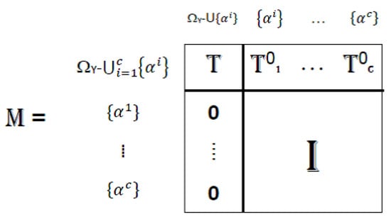 Figure A1. The transition probability matrix.( is the identity matrix, and is the zero matrix, all with the appropriate dimensions).
Step 3. Probability generating function
- 3.1
- For :
- Derive and using a probability product of maximum length b (a probability tree diagram may be useful).
- Derive the vector (the matrix may be helpful).
- Compute the vector (a probability tree diagram may be useful)
- Derive and by:
- Use the law of total expectation to obtain:
- 3.2
- The final is obtained by
References
- Schwager, S.J. Run probabilities in sequences of markov-dependent trials. J. Am. Stat. Assoc. 1983, 78, 168–175. [Google Scholar] [CrossRef]
- Karwe, V.V.; Naus, J.I. New recursive methods for scan statistic probabilities. Comput. Stat. Data Anal. 1997, 23, 389–402. [Google Scholar] [CrossRef]
- Martin, D.E.; Aston, J.A. Waiting time distribution of generalized later patterns. Comput. Stat. Data Anal. 2008, 52, 4879–4890. [Google Scholar] [CrossRef]
- Kulldorff, M. A spatial scan statistic. Commun. Stat. Theory Methods 1997, 26, 1481–1496. [Google Scholar] [CrossRef]
- Aki, S. Discrete distributions of order k on a binary sequence. Ann. Inst. Stat. Math. 1985, 37, 205–224. [Google Scholar] [CrossRef]
- Aki, S.; Hirano, K. Lifetime distribution and estimation problems of consecutive-k-out-of-n: f systems. Ann. Inst. Stat. Math. 1996, 48, 185–199. [Google Scholar] [CrossRef]
- Chang, Y.M.; Huang, T.H. Reliability of a 2-dimensional k-within consecutive-r’s-out-of-m’n: f system using finite markov chains. IEEE Trans. Reliab. 2010, 59, 725–733. [Google Scholar] [CrossRef]
- Dafnis, S.D.; Antzoulakos, D.L.; Philippou, A.N. Distributions related to (k1,k2) events. J. Stat. Plan. Inference 2010, 140, 1691–1700. [Google Scholar] [CrossRef]
- Dafnis, S.D.; Gounari, S.; Zotos, C.E.; Papadopoulos, G.K. The effect of cold periods on the biological cycle of Marchalina hellenica. Insects 2022, 13, 375. [Google Scholar] [CrossRef]
- Dafnis, S.D.; Makri, F.S.; Koutras, M.V. Generalizations of runs and patterns distributions for sequences of binary trials. Methodol. Comput. Appl. Probab. 2021, 23, 165–185. [Google Scholar] [CrossRef]
- Dafnis, S.D.; Makri, F.S.; Philippou, A.N. The reliability of a generalized consecutive system. Appl. Math. Comput. 2019, 359, 186–193. [Google Scholar] [CrossRef]
- Dafnis, S.D.; Makri, F.S. Distributions related to weak runs with a minimum and a maximum number of successes: A unified approach. Methodol. Comput. Appl. Probab. 2023, 25, 24. [Google Scholar] [CrossRef]
- Feller, W. An Introduction to Probability Theory and Its Applications, 3rd ed.; Wiley: New York, NY, USA, 1971; Volume 1. [Google Scholar]
- Philippou, A.N.; Georghiou, C.; Philippou, G.N. A generalized geometric distribution and some of its properties. Stat. Probab. Lett. 1983, 1, 171–175. [Google Scholar] [CrossRef]
- Philippou, A.N.; Makri, F.S. Successes, runs and longest runs. Stat. Probab. Lett. 1986, 4, 211–215. [Google Scholar] [CrossRef]
- Philippou, A.N.; Antzoulakos, D.L. Multivariate distributions of order k on a generalized sequence. Stat. Probab. Lett. 1990, 9, 453–463. [Google Scholar] [CrossRef]
- Ling, K. On geometric distributions of order (k1,k2,…,km). Stat. Probab. Lett. 1990, 9, 163–171. [Google Scholar] [CrossRef]
- Shmueli, G.; Cohen, A. Run-Related probability functions applied to sampling inspection. Technometrics 2000, 42, 188–202. [Google Scholar] [CrossRef]
- Koutras, M.V.; Eryilmaz, S. Compound geometric distribution of order k. Methodol. Comput. Appl. Probab. 2017, 19, 377–393. [Google Scholar] [CrossRef]
- Blom, G.; Thorburn, D. How many random digits are required until given sequences are obtained? J. Appl. Probab. 1982, 19, 518–531. [Google Scholar] [CrossRef]
- Ebneshahrashoob, M.; Sobel, M. Sooner and later waiting time problems for bernoulli trials: Frequency and run quotas. Stat. Probab. Lett. 1990, 9, 5–11. [Google Scholar] [CrossRef]
- Huang, W.T.; Tsai, C.S. On a modified binomial distribution of order k. Stat. Probab. Lett. 1991, 11, 125–131. [Google Scholar] [CrossRef]
- Makri, F.S. On occurrences of FS strings in linearly and circularly ordered binary sequences. J. Appl. Probab. 2010, 47, 157–178. [Google Scholar] [CrossRef]
- Kumar, A.N.; Upadhye, N.S. Generalizations of distributions related to (k1,k2)-runs. Metrika 2019, 82, 249–268. [Google Scholar] [CrossRef]
- Zhao, X.; Song, Y.; Wang, X.; Lv, Z. Distributions of (k1,k2,…,kl)-runs with multi-state Trials. Methodol. Comput. Appl. Probab. 2022, 24, 2689–2702. [Google Scholar] [CrossRef]
- Kong, Y. Multiple consecutive runs of multi-state trials: Distributions of (k1,k2,…,kl) patterns. J. Comput. Appl. Math. 2022, 403, 113846. [Google Scholar] [CrossRef]
- Chadjiconstantinidis, S.; Eryilmaz, S. Computing waiting time probabilities related to (k1,k2,…,kl) pattern. Stat. Pap. 2023, 64, 1373–1390. [Google Scholar] [CrossRef]
- Aki, S. Waiting time problems for a sequence of discrete random variables. Ann. Inst. Stat. Math. 1992, 44, 363–378. [Google Scholar] [CrossRef]
- Koutras, M.V. On a waiting time distribution in a sequence of bernoulli trials. Ann. Inst. Stat. Math. 1996, 48, 789–806. [Google Scholar] [CrossRef]
- Robin, S.; Daudin, J.J. Exact distribution of word occurrences in a random sequence of letters. J. Appl. Probab. 1999, 36, 179–193. [Google Scholar] [CrossRef]
- Aki, S.; Hirano, K. Waiting time problems for a two-dimensional pattern. Ann. Inst. Stat. Math. 2004, 56, 169–182. [Google Scholar] [CrossRef]
- Hirano, K.; Aki, S. On number of occurrences of success runs of specified length in a two-state markov chain. Stat. Sin. 1993, 3, 313–320. [Google Scholar]
- Fu, J.C.; Koutras, M.V. Distribution theory of runs: A markov chain approach. J. Am. Stat. Assoc. 1994, 89, 1050–1058. [Google Scholar] [CrossRef]
- Fu, J.C. Distribution theory of runs and patterns associated with a sequence of multi-state trials. Stat. Sin. 1996, 6, 957–974. [Google Scholar]
- Koutras, M.V. Waiting time distributions associated with runs of fixed length in two-state markov chains. Ann. Inst. Stat. Math. 1997, 49, 123–139. [Google Scholar] [CrossRef]
- Antzoulakos, D.L. Waiting times for patterns in a sequence of multistate trials. J. Appl. Probab. 2001, 38, 508–518. [Google Scholar] [CrossRef]
- Fisher, E.; Cui, S. Patterns generated by m-order markov chains. Stat. Probab. Lett. 2010, 80, 1157–1166. [Google Scholar] [CrossRef]
- Chang, Y.M.; Fu, J.C.; Lin, H.Y. Distribution and double generating function of number of patterns in a sequence of markov dependent multistate trials. Ann. Inst. Stat. Math. 2012, 64, 55–68. [Google Scholar] [CrossRef]
- Fu, J.C.; Chang, Y.M. On probability generating functions for waiting time distributions of compound patterns in a sequence of multistate trials. J. Appl. Probab. 2002, 39, 70–80. [Google Scholar] [CrossRef]
- Han, Q.; Hirano, K. Sooner and later waiting time problems for patterns in markov dependent trials. J. Appl. Probab. 2003, 40, 73–86. [Google Scholar] [CrossRef]
- Fu, J.C.; Lou, W.Y.W. Waiting time distributions of simple and compound patterns in a sequence of r-th order Markov dependent multi-state trials. Ann. Inst. Stat. Math. 2006, 58, 291–310. [Google Scholar] [CrossRef]
- Wu, T.L. Conditional waiting time distributions of runs and patterns and their applications. Ann. Inst. Stat. Math. 2020, 72, 531–543. [Google Scholar] [CrossRef]
- Aston, J.A.; Martin, D.E. Waiting time distributions of competing patterns in higher-order Markovian sequences. J. Appl. Probab. 2005, 42, 977–988. [Google Scholar] [CrossRef]
- Fu, J.C.; Lou, W.Y.W. Distribution Theory of Runs and Patterns and Its Applications: A Finite Markov Chain Imbedding Approach; World Scientific Publishing Co.: Singapore, 2003. [Google Scholar]
- Balakrishnan, N.; Koutras, M.V. Runs and Scans with Applications; John Wiley & Sons: Hoboken, NJ, USA, 2011. [Google Scholar]
- Aston, J.A.; Martin, D.E. Distributions associated with general runs and patterns in hidden Markov models. Ann. Appl. Stat. 2007, 1, 585–611. [Google Scholar] [CrossRef]
- Martin, D.E.K. Computation of exact probabilities associated with overlapping pattern occurrences. WIREs Comput. Stat. 2019, 11, e1477. [Google Scholar] [CrossRef]
- Martin, D.E.K. Distributions of pattern statistics in sparse markov models. Ann. Inst. Stat. Math. 2020, 72, 895–913. [Google Scholar] [CrossRef]
- Michael, B.V.; Eutichia, V. On the distribution of the number of success runs in a continuous time markov chain. Methodol. Comput. Appl. Probab. 2020, 22, 969–993. [Google Scholar] [CrossRef]
- Vaggelatou, E. On the longest run and the waiting time for the first run in a continuous time multi-state Markov chain. Methodol. Comput. Appl. Probab. 2024, 26, 55. [Google Scholar] [CrossRef]
- Makri, F.S.; Psillakis, Z.M. Distribution of patterns of constrained length in binary sequences. Methodol. Comput. Appl. Probab. 2023, 25, 90. [Google Scholar] [CrossRef]
- Makri, F.S.; Psillakis, Z.M.; Dafnis, S.D. Number of runs of ones of length exceeding a threshold in a modified binary sequence with locks. Commun. Stat. Simul. Comput. 2024, 1–17. [Google Scholar] [CrossRef]
- Inoue, K.; Aki, S. Generalized binomial and negative binomial distributions of order k by the l-overlapping enumeration scheme. Ann. Inst. Stat. Math. 2003, 55, 153–167. [Google Scholar] [CrossRef]
Disclaimer/Publisher’s Note: The statements, opinions and data contained in all publications are solely those of the individual author(s) and contributor(s) and not of MDPI and/or the editor(s). MDPI and/or the editor(s) disclaim responsibility for any injury to people or property resulting from any ideas, methods, instructions or products referred to in the content. |
© 2025 by the authors. Licensee MDPI, Basel, Switzerland. This article is an open access article distributed under the terms and conditions of the Creative Commons Attribution (CC BY) license (https://creativecommons.org/licenses/by/4.0/).