Advanced Fitted Mesh Finite Difference Strategies for Solving ‘n’ Two-Parameter Singularly Perturbed Convection–Diffusion System

Abstract

This paper proposes a robust finite difference method on a fitted Shishkin mesh to solve a system of n singularly perturbed convection–reaction–diffusion differential equations with two small parameters. Defined on the interval $[0,1]$, this system exhibits boundary layers due to the presence of small parameters, making accurate numerical approximations challenging. The method employs a piecewise uniform Shishkin mesh that adapts to layer regions and efficiently captures the solution’s behavior. The scheme is proven to be uniformly convergent with respect to the perturbation parameters, achieving nearly first-order accuracy. Comprehensive numerical experiments validate the theoretical results, illustrating the method’s robustness and efficiency in handling parameter-sensitive boundary layers.

1. Introduction

Singularly perturbed differential equations (SPDEs) are pivotal, with vastly different scales, arising in fields such as fluid dynamics, chemical kinetics, control systems and population dynamics [1,2]. Within this category, singularly perturbed differential equations (SPDEs) pose additional challenges due to the presence of small perturbation parameters, which induce boundary layers. The accurate numerical approximation of these layers is complex, especially because of the two parameters. Various approaches, including fitted mesh [3] and fitted operator methods [4], have been developed to tackle SPDEs. The mesh used in the proposed scheme is based on the Shishkin mesh, introduced in [3]. This type of mesh has been widely used in singularly perturbed problems to ensure parameter-uniform convergence. Cen [5] demonstrated a hybrid approach using Shishkin meshes to achieve near-second-order convergence, while Gracia et al. [6] introduced a monotone method for SPDEs with two parameters affecting both convection and diffusion. Some of the pioneering and recent works in this field are [7,8,9,10,11,12]. However, SPDEs governed by multiple small parameters, often denoted as $\mu$ and ${ϵ}_i(i=1,2,\cdots ,n)$, introduce unique challenges. Specifically, the interactions between these parameters produce intricate boundary layers, often governed by the ratio ${\mu }^2/{ϵ}_i$, requiring parameter-robust methods for accurate representation. In this work, we propose a fitted mesh finite difference method designed to be parameter-robust for SPDEs, particularly as both $\mu$ and ${ϵ}_i$ tend toward zero. The theoretical analysis establishes stability and bounds for the solution’s derivatives, demonstrating that the proposed method achieves nearly first-order accuracy uniformly with respect to both parameters. The main contribution of this paper is the development of a robust, parameter-insensitive numerical scheme for an n-system of SPDEs in a convection–diffusion–reaction framework. Our approach addresses a broader class of problems than previous studies that focused on either scalar singularly perturbed delay differential equations with two parameters [13], two systems of singularly perturbed equations without delay terms [14] and a system of two singularly perturbed differential equations with delay terms and two parameters [15]. A key novelty of this paper is its ability to handle the complex interaction between two distinct perturbation parameters affecting the convection and diffusion terms in an n-system of equations. This work advances the numerical analysis of SPDEs by providing a robust scheme that accurately resolves boundary layers, even under two parameter conditions and achieve parameter-uniform convergence, significantly enhancing the numerical analysis of SPDEs.

2. Formulation of the Problem

The following system of singularly perturbed two-parameter differential equations is under consideration

$$E{\overrightarrow{u}}^{\prime \prime }\left(x\right)+\mu \mathit{A}\left(x\right){\overrightarrow{u}}^{\prime }\left(x\right)-\mathcal{B}\left(x\right)\overrightarrow{u}\left(x\right)=\overrightarrow{\mathit{f}}\left(x\right)\mathrm{for}\mathrm{all}x\in \Omega =(0,1),$$

(1)

$$\overrightarrow{u}\left(0\right)=\overrightarrow{\phi },\overrightarrow{u}\left(1\right)=\overrightarrow{\ell }.$$

Here, $\overrightarrow{u}=\left(\begin{array}{c}{u}_1\\ u_2\\ ⋮\\ u_n\end{array}\right),\overrightarrow{\mathit{f}}=\left(\begin{array}{c}{f}_1\\ f_2\\ ⋮\\ f_n\end{array}\right),$ $E=\left(\begin{array}{cccc}{ϵ}_1& 0& \cdots & 0\\ 0& {ϵ}_2& \cdots & 0\\ ⋮& ⋮& \ddots & ⋮\\ 0& 0& \cdots & {ϵ}_n\end{array}\right),$

$$\mathit{A}\left(x\right)=\left(\begin{array}{cccc}{\mathfrak{a}}_1\left(x\right)& 0& \cdots & 0\\ 0& {\mathfrak{a}}_2\left(x\right)& \cdots & 0\\ ⋮& ⋮& \ddots & ⋮\\ 0& 0& \cdots & {\mathfrak{a}}_n\left(x\right)\end{array}\right),\mathcal{B}\left(x\right)=\left(\begin{array}{cccc}{\mathfrak{b}}_{11}\left(x\right)& -{\mathfrak{b}}_{12}\left(x\right)& \cdots & -{\mathfrak{b}}_{1n}\left(x\right)\\ -{\mathfrak{b}}_{21}\left(x\right)& {\mathfrak{b}}_{22}\left(x\right)& \cdots & -{\mathfrak{b}}_{2n}\left(x\right)\\ ⋮& ⋮& \ddots & ⋮\\ -{\mathfrak{b}}_{n1}\left(x\right)& -{\mathfrak{b}}_{n2}\left(x\right)& \cdots & {\mathfrak{b}}_{nn}\left(x\right)\end{array}\right),$$

where ${ϵ}_i$, for $i=1,2,\cdots ,n$, satisfying $0<{ϵ}_1<{ϵ}_2<\cdots <{ϵ}_n\le 1$, and $\mu$, satisfying $0<\mu \le 1$, are small parameters. The functions ${\mathfrak{a}}_i\left(x\right)$, ${\mathfrak{b}}_{ij}\left(x\right)$ and $f_i\left(x\right)$ act as coefficients, which are all sufficiently smooth over the domain $\overline{\Omega }=[0,1]$, and ${\mathfrak{a}}_i\left(x\right)\ge \alpha >0,{\mathfrak{b}}_{ii}\left(x\right)-{\sum }_{j=1}^n{\mathfrak{b}}_{ij}\left(x\right)\ge \beta >0,{\mathfrak{b}}_{ij}\left(x\right)>0,$ $\mathrm{for}i,j=1,2,\cdots ,n\mathrm{and}i\ne j.$ The value of $\gamma$ is determined as

$$\gamma =\underset{x\in \overline{\Omega }}{min}\left({\displaystyle \frac{{\mathfrak{b}}_{ii}\left(x\right)-{\sum }_{j=1}^n{\mathfrak{b}}_{ij}\left(x\right)}{{\mathfrak{a}}_i\left(x\right)}}\right)\mathrm{for}i=1,2,\cdots ,n\mathrm{and}i\ne j.$$

When $\mu =0$, the above problem is considered in [16]. The problem demonstrates boundary layers influenced by both ${ϵ}_i$ and $\mu$; in particular, the layers are influenced by the ratio of ${\displaystyle \frac{{\mu }^2}{{ϵ}_i}}$. If ${\displaystyle \frac{{\mu }^2}{{ϵ}_i}}\le {\displaystyle \frac{\gamma }{\alpha }}$, $1\le i\le n$, the reduced problem can be expressed as

$$-\mathcal{B}\left(x\right)\overrightarrow{u}\left(x\right)=\overrightarrow{\mathit{f}}\left(x\right),x\in (0,1].$$

(2)

This predicts a boundary layer of width $O\left(\sqrt{{ϵ}_i}\right)$ near $x=0$, assuming $\overrightarrow{u}\left(0\right)\ne \overrightarrow{\phi }\left(0\right)$. A similar boundary layer of width $O\left(\sqrt{{ϵ}_i}\right)$ is expected near $x=1$, if $\overrightarrow{u}\left(1\right)\ne \overrightarrow{\ell }$. If ${\displaystyle \frac{{\mu }^2}{{ϵ}_j}}\ge {\displaystyle \frac{\gamma }{\alpha }}$, $1<i<j\le n$, the reduced problem is

$$\mu \mathbf{A}\left(x\right){\overrightarrow{u}}^{\prime }\left(x\right)-\mathcal{B}\left(x\right)\overrightarrow{u}\left(x\right)=\overrightarrow{\mathit{f}}\left(x\right),x\in (0,1),$$

(3)

with boundary conditions $\overrightarrow{u}\left(x\right)=\overrightarrow{\phi }\left(x\right)\mathrm{on}[-1,0],\overrightarrow{u}\left(1\right)=\overrightarrow{\ell }.$ This problem remains singularly perturbed with the parameter $\mu$. A boundary layer of width $O\left(\mu \right)$ is anticipated near $x=1$. Additionally, a boundary layer of width $O\left({\displaystyle \frac{{ϵ}_i}{\mu }}\right)$ is anticipated near $x=0$, if $\overrightarrow{u}\left(0\right)\ne \overrightarrow{\phi }\left(0\right)$. Numerical experiments suggest that the interior right layer weakens considerably when ${ϵ}_i\ll {\mu }^2$.

3. Analytical Results

This section presents a minimum principle, establishes a stability result and derives estimates for the derivatives of the solution associated with the problem defined by Equation (1).

Lemma 1. 

Let $\overrightarrow{\mathit{\psi }}={({\mathit{\psi }}_1,{\mathit{\psi }}_2,\cdots ,{\mathit{\psi }}_n)}^T$ be such that $\overrightarrow{\mathit{\psi }}\left(0\right)\ge \overrightarrow{0}$, $\overrightarrow{\mathit{\psi }}\left(1\right)\ge \overrightarrow{0}$ and $\overrightarrow{L}\overrightarrow{\mathit{\psi }}\le \overrightarrow{0}$ on $(0,1)$; then, $\overrightarrow{\mathit{\psi }}\ge \overrightarrow{0}$ on $[0,1]$.

Proof. 

Assume $x^{*}$ and $s^{*}$ are such that ${\displaystyle {\mathit{\psi }}_{s^{*}}\left(x^{*}\right)=\underset{x\in \Omega ,s=1,2,\cdots ,n}{min}{\mathit{\psi }}_s\left(x\right)}$. Suppose ${\mathit{\psi }}_{s^{*}}\left(x^{*}\right)<0$. Then, $x^{*}$ cannot be at the boundaries 0 or 1. At $x^{*}$, the first derivative of ${\mathit{\psi }}_{s^{*}}$ denoted as ${\mathit{\psi }}_{s^{*}}^{\prime }\left(x^{*}\right)=0$ and the second derivative ${\mathit{\psi }}_{s^{*}}^{\prime \prime }\left(x^{*}\right)\ge 0$.

Claim: $x^{*}\notin (0,1)$. If $x^{*}\in (0,1)$, then

$${\left(\overrightarrow{L}\overrightarrow{\mathit{\psi }}\right)}_{s^{*}}\left(x^{*}\right)={ϵ}_{s^{*}}{\mathit{\psi }}_{s^{*}}^{\prime \prime }\left(x^{*}\right)+\mu {\mathfrak{a}}_{s^{*}}\left(x^{*}\right){\mathit{\psi }}_{s^{*}}^{\prime }\left(x^{*}\right)-\sum _{j=1}^n{\mathfrak{b}}_{s^{*}j}\left(x^{*}\right){\mathit{\psi }}_j\left(x^{*}\right)>0,$$

which contradicts the assumption that $\overrightarrow{L}\overrightarrow{\mathit{\psi }}\le \overrightarrow{0}$ on $(0,1)$. Thus, $x^{*}\notin (0,1)$. Therefore, $\overrightarrow{\mathit{\psi }}\ge \overrightarrow{0}$ on $[0,1]$. The proof of the lemma is complete. □

Lemma 2. (Stability Result)

Let $\overrightarrow{\mathit{\psi }}\in C^2\left(\overline{\Omega }\right)$; for $x\in \overline{\Omega }$,

$$|{\mathit{\psi }}_i\left(x\right)|\le max\left\{|\overrightarrow{\mathit{\psi }}\left(0\right)|,|\overrightarrow{\mathit{\psi }}\left(1\right)|,{\displaystyle \frac{1}{\beta }}{\parallel \overrightarrow{L}\overrightarrow{\mathit{\psi }}\parallel }_{\Omega }\right\}.$$

Proof. 

Define

$$M=max\left\{|\overrightarrow{\mathit{\psi }}\left(0\right)|,|\overrightarrow{\mathit{\psi }}\left(1\right)|,{\displaystyle \frac{1}{\beta }}{\parallel \overrightarrow{L}\overrightarrow{\mathit{\psi }}\parallel }_{\Omega }\right\}.$$

Consider the functions ${\overrightarrow{\theta }}^{\pm }\left(x\right)=M\overrightarrow{e}\pm \overrightarrow{\mathit{\psi }}\left(x\right)$, where $\overrightarrow{e}={(1,1,\cdots ,1)}^T$. Clearly, ${\overrightarrow{\theta }}^{\pm }\left(0\right)\ge \overrightarrow{0}$, ${\overrightarrow{\theta }}^{\pm }\left(1\right)\ge \overrightarrow{0}$ and $\overrightarrow{L}{\overrightarrow{\theta }}^{\pm }\left(x\right)\le \overrightarrow{0}$ for all $x\in \Omega$. Hence, by Lemma 1, it is proven that $|{\mathit{\psi }}_i\left(x\right)|\le M$, which yields the required result. □

Theorem 1. 

Let $\overrightarrow{u}$ be the solution of Equation (1), and then its derivatives satisfy the following bounds on Ω,

$$|u_i^{\left(k\right)}\left(x\right)|\le {\displaystyle \frac{C}{{\left({\sqrt{ϵ}}_i\right)}^k}}\left(1+{\left({\displaystyle \frac{\mu }{\sqrt{{ϵ}_i}}}\right)}^k\right)max\{\parallel \overrightarrow{u}\parallel ,\parallel \overrightarrow{f}\parallel \},$$

(4)

$$\left|{u_i}^{\left(3\right)}\left(x\right)\right|\le {\displaystyle \frac{C}{{\left(\sqrt{{ϵ}_i}\right)}^3}}\left(1+{\left({\displaystyle \frac{\mu }{\sqrt{{ϵ}_i}}}\right)}^3\right)max\left\{\parallel \overrightarrow{u}\parallel ,\parallel \overrightarrow{f}\parallel ,\parallel {\overrightarrow{f}}^{\prime }\parallel \right\},$$

(5)

$$|u_i^{\left(4\right)}\left(x\right)|\le {\displaystyle \frac{C}{{\left(\sqrt{{ϵ}_i}\right)}^4}}\left(1+{\left({\displaystyle \frac{\mu }{\sqrt{{ϵ}_i}}}\right)}^4\right)max\left\{\parallel \overrightarrow{u}\parallel ,\parallel \overrightarrow{f}\parallel ,\parallel {\overrightarrow{f}}^{\prime }\parallel ,\parallel {\overrightarrow{f}}^{\prime \prime }\parallel \right\}$$

(6)

where the constant C is independent of ${ϵ}_i$ and μ, $i=1,2,\cdots ,n$ and $k=1,2.$

Proof. 

The proof follows the methodology outlined in Lemma 2.2 of [11]. For any $x\in (0,1)$, a neighborhood $N_p=(p,p+\sqrt{{ϵ}_i})$ such that $x\in N_p$ and $N_p\subset (0,1)$. According to the mean value theorem, there exists a $y\in N_p$ satisfying

$$u_i^{\prime }\left(y\right)={\displaystyle \frac{u_i(p+\sqrt{{ϵ}_i})-u_i\left(p\right)}{\sqrt{{ϵ}_i}}}\Rightarrow |u_i^{\prime }\left(y\right)|\le {\displaystyle \frac{2\parallel u_i\parallel }{\sqrt{{ϵ}_i}}}.$$

Now,

$$u_i^{\prime }\left(x\right)=u_i^{\prime }\left(y\right)+{\int }_y^x{u}_i^{\prime \prime }\left(\eta \right)d\eta .$$

Thus,

$$|u_i^{\prime }\left(x\right)|\le {\displaystyle \frac{C}{{\sqrt{ϵ}}_i}}\left(1+{\displaystyle \frac{\mu }{{\sqrt{ϵ}}_i}}\right)max\{\parallel \overrightarrow{u}\parallel ,\parallel \overrightarrow{f}\parallel \}.$$

The bounds for $u_i^{\prime \prime }$ are obtained from Equation (1). Similarly, the bounds of $u_i^{\prime \prime \prime }$ and $u_i^{\left(iv\right)}$ can be established for higher-order derivatives through analogous corresponding manipulations. The proof of the theorem is complete. □

4. Shishkin Decomposition of the Solution

For each of the cases $\alpha {\mu }^2\le \gamma {ϵ}_i$ and $\alpha {\mu }^2\ge \gamma {ϵ}_j$, $\overrightarrow{u}$ is expressed by

$$\overrightarrow{u}=\overrightarrow{v}+{\overrightarrow{w}}^L+{\overrightarrow{w}}^R,$$

(7)

where

$${\overrightarrow{w}}^L\left(x\right)=\left\{\begin{array}{c}{w_1}^L\left(x\right)\hfill \\ {w_2}^L\left(x\right)\hfill \\ ⋮\hfill \\ {w_n}^L\left(x\right)\hfill \end{array}\right.,\mathrm{for}x\in [0,1],{\overrightarrow{w}}^R\left(x\right)=\left\{\begin{array}{c}{w_1}^R\left(x\right)\hfill \\ {w_2}^R\left(x\right)\hfill \\ ⋮\hfill \\ {w_n}^R\left(x\right)\hfill \end{array}\right.,\mathrm{for}x\in [0,1].$$

(8)

Case (i): $\alpha {\mu }^2\le \gamma {ϵ}_i$

In this case, for $1\le i\le n$,

$$\begin{array}{cc}\hfill \overrightarrow{L}\overrightarrow{v}\left(x\right)& =\overrightarrow{f}\left(x\right),\mathrm{for}x\in (0,1),\overrightarrow{v}\left(0\right)\mathrm{and}\overrightarrow{v}\left(1\right)\mathrm{are}\mathrm{selected},\hfill \end{array}$$

(9)

$$\begin{array}{cc}\hfill \overrightarrow{L}{\overrightarrow{w}}^L\left(x\right)& =\overrightarrow{0},\mathrm{for}x\in (0,1),{\overrightarrow{w}}^L\left(0\right)=\overrightarrow{u}\left(0\right)-\overrightarrow{v}\left(0\right)-c({ϵ}_i,\mu ),{\overrightarrow{w}}^L\left(1\right)=\overrightarrow{0},\hfill \end{array}$$

(10)

$$\begin{array}{cc}\hfill \overrightarrow{L}{\overrightarrow{w}}^R\left(x\right)& =\overrightarrow{0},\mathrm{for}x\in (0,1),{\overrightarrow{w}}^R\left(0\right)=c({ϵ}_i,\mu ),{\overrightarrow{w}}^R\left(1\right)=k({ϵ}_i,\mu ).\hfill \end{array}$$

(11)

Case (ii): $\alpha {\mu }^2\ge \gamma {ϵ}_j$

Inthis case, for $1<i<j\le n$,

$$\begin{array}{cc}\hfill \overrightarrow{L}\overrightarrow{v}\left(x\right)& =\overrightarrow{f}\left(x\right),\mathrm{for}x\in (0,1),\overrightarrow{v}\left(0\right)\mathrm{and}\overrightarrow{v}\left(1\right)\mathrm{are}\mathrm{selected},\hfill \end{array}$$

(12)

$$\begin{array}{cc}\hfill \overrightarrow{L}{\overrightarrow{w}}^L& =\overrightarrow{0},\mathrm{for}x\in (0,1),{\overrightarrow{w}}^L\left(0\right)=\overrightarrow{u}\left(0\right)-\overrightarrow{v}\left(0\right)-c({ϵ}_i,\mu ),{\overrightarrow{w}}^L\left(1\right)=\overrightarrow{0},\hfill \end{array}$$

(13)

$$\begin{array}{cc}\hfill \overrightarrow{L}{\overrightarrow{w}}^R& =\overrightarrow{0},\mathrm{for}x\in (0,1),{\overrightarrow{w}}^R\left(0\right)=c({ϵ}_i,\mu ),{\overrightarrow{w}}^R\left(1\right)=k({ϵ}_i,\mu ).\hfill \end{array}$$

(14)

It should be ensured that the constants $k({ϵ}_i,\mu )$ are selected appropriately. Additionally, the constants $c({ϵ}_i,\mu )$ should be determined independently for the cases $\alpha {\mu }^2\le \gamma {ϵ}_i$ and $\alpha {\mu }^2\ge \gamma {ϵ}_j$, ensuring they meet the bounds required for the singular component. Given that $\overrightarrow{u}\left(0\right)$ and $\overrightarrow{u}\left(1\right)$ are bounded by constants that do not depend on ${ϵ}_i$ and $\mu$, even though c and k are functions of ${ϵ}_i$ and $\mu$, the magnitudes $|c|$ and $|k|$ are constants independent of ${ϵ}_i$ and $\mu$.

5. Bounds on the Regular Component and Its Derivatives

To establish the result, bounds for the smooth components and their derivatives on the interval $[0,1]$ should be estimated. Specifically, this is achieved by decomposing each component with respect to ${ϵ}_n$, and then applying ${ϵ}_{n-1}$ to the first $n-1$ components, followed by ${ϵ}_{n-2}$ for the first $n-2$ components, and so on. This step-by-step decomposition approach is as follows for both cases.

Case (i): $\alpha {\mu }^2\le \gamma {ϵ}_i$

Establishing the bounds of the regular component $\overrightarrow{v}$, it is broken down as

$$\overrightarrow{v}={\overrightarrow{y}}_n+\sqrt{{ϵ}_n}{\overrightarrow{z}}_n+{\sqrt{{ϵ}_n}}^2{\overrightarrow{q}}_n+{\sqrt{{ϵ}_n}}^3{\overrightarrow{p}}_n.$$

Here, ${\overrightarrow{y}}_n={(y_{n1},y_{n2},...,y_{nn})}^T$ represents the solution

$$\begin{array}{cc}\hfill -{\mathcal{B}}_{\mathbf{n}}\left(x\right){\overrightarrow{y}}_n\left(x\right)& =\overrightarrow{\mathit{f}}\left(x\right),\mathrm{for}x\in [0,1],\hfill \end{array}$$

(15)

where ${\overrightarrow{z}}_n={(z_{n1},z_{n2},...,z_{nn})}^T$ is the solution of

$$\begin{array}{cc}\hfill {\mathcal{B}}_{\mathit{n}}\left(x\right){\overrightarrow{z}}_n\left(x\right)& ={\sqrt{ϵ}}_n^{-1}E{\overrightarrow{y}}_n^{\prime \prime }+\mu {\sqrt{ϵ}}_n^{-1}{\mathit{A}}_{\mathit{n}}{\overrightarrow{y}}_n^{\prime },forx\in [0,1],\hfill \end{array}$$

(16)

${\overrightarrow{q}}_n={(q_{n1},q_{n2},...,q_{nn})}^T$ represents the solution of

$$\begin{array}{cc}\hfill {\mathcal{B}}_{\mathit{n}}\left(x\right){\overrightarrow{q}}_n\left(x\right)& ={\sqrt{ϵ}}_n^{-1}E{\overrightarrow{z}}_n^{\prime \prime }+\mu {\sqrt{ϵ}}_n^{-1}{\mathit{A}}_{\mathit{n}}{\overrightarrow{z}}_n^{\prime },\mathrm{for}x\in [0,1],\hfill \end{array}$$

(17)

and ${\overrightarrow{p}}_n={(p_{n1},p_{n2},...,p_{nn})}^T$ is the solution of

$$\overrightarrow{L}{\overrightarrow{p}}_n\left(x\right)={\sqrt{ϵ}}_n^{-1}E{\overrightarrow{q}}_n^{\prime \prime }+\mu {\sqrt{ϵ}}_n^{-1}{\mathit{A}}_{\mathit{n}}{\overrightarrow{q}}_n^{\prime }\mathrm{on}(0,1).$$

(18)

Since ${\sqrt{{ϵ}_n}}^{-1}E$ is a matrix whose entries are bounded, for $0\le k\le 3$,

$$\Vert {\overrightarrow{y}}_n^{\left(k\right)}\Vert \le C,\Vert {\overrightarrow{z}}_n^{\left(k\right)}\Vert \le C,\Vert {\overrightarrow{q}}_n^{\left(k\right)}\Vert \le C.$$

(19)

Now, using Theorem 1 and (18) for the choice of $p_{nn}\left(0\right)=0,$,

$$\begin{array}{c}\hfill |p_{nn}^{\left(k\right)}|\le C{\sqrt{ϵ}}_n^{-k}.\end{array}$$

(20)

Then, from (19) and (20), it is found that

$$\begin{array}{c}\hfill |v_n^{\left(k\right)}|\le C(1+{\left({\sqrt{ϵ}}_n\right)}^{3-k}).\end{array}$$

(21)

In order to facilitate the estimation of bounds $v_i^{\left(k\right)}$ for $1\le i\le n-1$, the following representation is introduced, for $1\le l\le n$, $E_l=\left[\begin{array}{cccc}{ϵ}_1& 0& \cdots & 0\\ 0& {ϵ}_2& \cdots & 0\\ ⋮& ⋮& \ddots & ⋮\\ 0& 0& \cdots & {ϵ}_l\end{array}\right],$ ${\mathit{A}}_{\mathit{l}}=\left[\begin{array}{cccc}{\mathfrak{a}}_1& 0& \cdots & 0\\ 0& {\mathfrak{a}}_2& \cdots & 0\\ ⋮& ⋮& \ddots & ⋮\\ 0& 0& \cdots & {\mathfrak{a}}_l\end{array}\right],$ ${\mathcal{B}}_{\mathit{l}}=\left[\begin{array}{cccc}{\mathfrak{b}}_{11}& -{\mathfrak{b}}_{12}& \cdots & -{\mathfrak{b}}_{1l}\\ -{\mathfrak{b}}_{21}& {\mathfrak{b}}_{22}& \cdots & -{\mathfrak{b}}_{2l}\\ ⋮& ⋮& \ddots & ⋮\\ -{\mathfrak{b}}_{l1}& -{\mathfrak{b}}_{l2}& \cdots & {\mathfrak{b}}_{ll}\end{array}\right],$ ${\overrightarrow{\tilde{p}}}_l={(p_{l1},p_{l2},\cdots ,p_{l(l-1)})}^T,{\overrightarrow{g}}_{(l-1)}={(g_{(l-1)1},g_{(l-1)2},\cdots ,g_{(l-1)(l-1)})}^T,$ with $g_{(l-1)j}=-{\displaystyle \frac{{ϵ}_j}{{\sqrt{ϵ}}_l}}{q}_{lj}^{\prime \prime }+{\displaystyle \frac{\mu }{{\sqrt{ϵ}}_l}}{\mathit{A}}_{\mathit{l}}{q}_{lj}^{\prime }+{\mathfrak{b}}_{jl}{p}_{ll}$. To proceed with the analysis, consider the system of first $n-1$ equations in (18),

$${\overrightarrow{\tilde{L}}}_n{\overrightarrow{\tilde{p}}}_n\equiv E_{n-1}{\overrightarrow{\tilde{p}}}_n^{\prime \prime }\left(x\right)+{\mathit{A}}_{n-1}\left(x\right){\overrightarrow{\tilde{p}}}_n^{\prime }\left(x\right)-{\mathcal{B}}_{n-1}\left(x\right){\overrightarrow{\tilde{p}}}_n\left(x\right)={\overrightarrow{g}}_{n-1}\left(x\right).$$

The decomposition of ${\overrightarrow{\tilde{p}}}_n$ proceeds similarly to the equation above,

$${\overrightarrow{\tilde{p}}}_n={\overrightarrow{y}}_{n-1}+\sqrt{{ϵ}_{n-1}}{\overrightarrow{z}}_{n-1}+{\sqrt{{ϵ}_{n-1}}}^2{\overrightarrow{q}}_{n-1}+{\sqrt{{ϵ}_{n-1}}}^3{\overrightarrow{p}}_{n-1}.$$

Proceeding similarly to above, the problem associated with ${\overrightarrow{p}}_n$ is similar to that in (18). By applying the estimates, the bound on the solution is obtained for $0\le k\le 3$, $\parallel {\overrightarrow{y}}_{n-1}^{\left(k\right)}\parallel \le C(1+{\left({\sqrt{ϵ}}_n\right)}^{1-k}),$ $\parallel {\overrightarrow{z}}_{n-1}^{\left(k\right)}\parallel \le C{\left({\sqrt{ϵ}}_n\right)}^{-k},$ $\parallel {\overrightarrow{q}}_{n-1}^{\left(k\right)}\parallel \le C{\left({\sqrt{ϵ}}_n\right)}^{-k-1}$. Then, using Theorem 1 and ${\overrightarrow{q}}_{n-1}^{\left(k\right)}$, $|p_{(n-1)(n-1)}^{\left(k\right)}|\le C{\sqrt{ϵ}}_n^{-3}{\sqrt{ϵ}}_{n-1}^{-k}$. Therefore, $|v_{n-1}^{\left(k\right)}|\le C(1+{\left({\sqrt{ϵ}}_{n-1}\right)}^{3-k}).$ Employing a similar approach, singularly perturbed systems of l equations can be formulated, where $l=n-2,n-3,\cdots ,2,1$,

$${\overrightarrow{\tilde{L}}}_{l+1}{\overrightarrow{\tilde{p}}}_{l+1}\equiv E_l{\overrightarrow{\tilde{p}}}_{l+1}^{\prime \prime }\left(x\right)+{\mathit{A}}_l\left(x\right){\overrightarrow{\tilde{p}}}_{l+1}^{\prime }\left(x\right)-{\mathcal{B}}_l\left(x\right){\overrightarrow{\tilde{p}}}_{l+1}\left(x\right)={\overrightarrow{g}}_l\left(x\right).$$

Applying a similar decomposition yields $|v_l^{\left(k\right)}|\le C(1+{\left({\sqrt{ϵ}}_l\right)}^{3-k}).$ For each i, where $1\le i\le n$ and $0\le k\le 3$, the bound is

$$\begin{array}{c}\hfill |v_i^{\left(k\right)}|\le C(1+{\left({\sqrt{ϵ}}_i\right)}^{3-k}).\end{array}$$

(22)

Case (ii): $\alpha {\mu }^2\ge \gamma {ϵ}_j$

Establishing the bounds of the regular component $\overrightarrow{v}$, it is broken down as

$$\overrightarrow{v}={\overrightarrow{y}}_n+{ϵ}_n{\overrightarrow{z}}_n+{ϵ}_n^2{\overrightarrow{q}}_n+{ϵ}_n^3{\overrightarrow{p}}_n.$$

urthermore, the maximum principle for a linear operator of first order in the context of a terminal value problem has been demonstrated. Define the operators

$$\begin{array}{cc}\hfill {\overrightarrow{L}}_1& \equiv \mu \mathit{A}\left(x\right){\overrightarrow{u}}^{\prime }\left(x\right)-\mathcal{B}\left(x\right)\overrightarrow{u}\left(x\right).\hfill \end{array}$$

(23)

By decomposing ${\overrightarrow{y}}_n,{\overrightarrow{z}}_n,{\overrightarrow{q}}_n$ individually and proceeding similarly to case (i), for $1\le i\le n$ and $0\le k\le 3$, the bound is determined as follows

$$\begin{array}{c}\hfill |v_i^{\left(k\right)}|\le C(1+{ϵ}_i^{3-k}{\mu }^{k-3}).\end{array}$$

(24)

6. Layer Functions

The functions for the layers are denoted by ${\mathfrak{B}}_i^l\left(x\right)$ and ${\mathfrak{B}}_i^r\left(x\right)$; $1\le i\le n$ is specified over the interval $[0,1]$

$$\begin{array}{c}\hfill {\mathfrak{B}}_i^l\left(x\right)=\left\{\begin{array}{cc}{e}^{-{\theta }_{i}x},\hfill & \alpha {\mu }^2\le \gamma {ϵ}_i\hfill \\ e^{-{\lambda }_{i}x},\hfill & \alpha {\mu }^2\ge \gamma {ϵ}_j\hfill \end{array}\right.,{\mathfrak{B}}_i^r\left(x\right)=\left\{\begin{array}{cc}{e}^{-{\theta }_i(1-x)},\hfill & \alpha {\mu }^2\le \gamma {ϵ}_i\hfill \\ e^{-\kappa (1-x)},\hfill & \alpha {\mu }^2\ge \gamma {ϵ}_j\hfill \end{array}\right.,\end{array}$$

(25)

where ${\theta }_i=\sqrt{{\displaystyle \frac{\gamma \alpha }{{ϵ}_i}}}$; ${\lambda }_i={\displaystyle \frac{\alpha \mu }{{ϵ}_i}}$; and $\kappa ={\displaystyle \frac{\gamma }{2\mu }}$, for $1\le i\le n$. Following Lemma 5 presented in [16], the points $x_s\in \left(0,{\displaystyle \frac{1}{2}}\right)$, which satisfy the conditions ${\mathfrak{B}}_i^l,{\mathfrak{B}}_j^l,{\mathfrak{B}}_i^r,{\mathfrak{B}}_j^r,1\le i<j\le n$ for the case $\alpha {\mu }^2\le \gamma {ϵ}_i$, can be proved.

$${\displaystyle \frac{{\mathfrak{B}}_i^l\left(x_{i,j}^{\left(k\right)}\right)}{{ϵ}_i^k}}={\displaystyle \frac{{\mathfrak{B}}_j^l\left(x_{i,j}^{\left(k\right)}\right)}{{ϵ}_j^k}}\mathrm{on}[0,1],{\displaystyle \frac{{\mathfrak{B}}_i^r(1-x_{i,j}^{\left(k\right)})}{{ϵ}_i^k}}={\displaystyle \frac{{\mathfrak{B}}_j^r(1-x_{i,j}^{\left(k\right)})}{{ϵ}_j^k}}\mathrm{on}[0,1],0\le k\le 2.$$

Similarly, for the case $\alpha {\mu }^2\ge \gamma {ϵ}_j$, it can be demonstrated that there exist points $x_{i,j}^{\left(s\right)},$$s=1,2,3$ in $\left(0,{\displaystyle \frac{1}{2}}\right)$ such that

$${\displaystyle \frac{{\mathfrak{B}}_i^l\left(x_{i,j}^{\left(s\right)}\right)}{{ϵ}_i^s}}={\displaystyle \frac{{\mathfrak{B}}_j^l\left(x_{i,j}^{\left(s\right)}\right)}{{ϵ}_j^s}}.$$

7. Bounds on the Singular Component and Its Derivatives

Theorem 2. 

Let ${\overrightarrow{w}}^L,{\overrightarrow{w}}^R$ satisfy problems (10) and (11) and (13) and (14) for the cases $\alpha {\mu }^2\le \gamma {ϵ}_i$ and $\alpha {\mu }^2\ge \gamma {ϵ}_j$, respectively. Consequently, the components of ${\overrightarrow{w}}^L$ and ${\overrightarrow{w}}^R$ satisfy the following bounds on $(0,1)$. For the case $\alpha {\mu }^2\le \gamma {ϵ}_i,1\le i\le n$,

$$\begin{array}{cc}\hfill |w_i^L\left(x\right)|\le & C{\mathfrak{B}}_n^l\left(x\right),\hfill \\ \hfill |w_i^{L,\left(1\right)}\left(x\right)|& \le C\left({ϵ}_i^{-1/2}{\mathfrak{B}}_i^l\left(x\right)+{ϵ}_n^{-1/2}{\mathfrak{B}}_n^l\left(x\right)\right),\hfill \\ \hfill |w_i^{L,\left(2\right)}\left(x\right)|& {\displaystyle \le C\sum _{k=i}^n{ϵ}_k^{-1/2}{\mathfrak{B}}_k^l\left(x\right),}\hfill \\ \hfill |w_i^{L,\left(3\right)}\left(x\right)|& \le C{ϵ}_i^{-1}\left({\displaystyle \sum _{k=1}^{i-1}{ϵ}_k^{-1/2}{\mathfrak{B}}_k^l\left(x\right)+\sum _{k=i}^n{ϵ}_k^{-1/2}{\mathfrak{B}}_k^l\left(x\right)}\right).\hfill \end{array}$$

For the case $\alpha {\mu }^2\ge \gamma {ϵ}_j,1\le i<j\le n$,

$$\begin{array}{cc}\hfill |w_i^L\left(x\right)|\le & C{\mathfrak{B}}_n^l\left(x\right),\hfill \\ \hfill |w_i^{L,\left(1\right)}\left(x\right)|& \le C\mu \left({ϵ}_i^{-1}{\mathfrak{B}}_i^l\left(x\right)+{ϵ}_n^{-1}{\mathfrak{B}}_n^l\left(x\right)\right),\hfill \\ \hfill |w_i^{L,\left(2\right)}\left(x\right)|& {\displaystyle \le C{\mu }^2\sum _{k=j}^n{ϵ}_k^{-2}{\mathfrak{B}}_k^l\left(x\right),}\hfill \\ \hfill |w_i^{L,\left(3\right)}\left(x\right)|& \le C{\mu }^3\left({\displaystyle {ϵ}_i^{-1}\sum _{k=1}^{j-1}{ϵ}_k^{-2}{\mathfrak{B}}_k^l\left(x\right)+\sum _{k=j}^n{ϵ}_k^{-3}{\mathfrak{B}}_k^l\left(x\right)}\right).\hfill \end{array}$$

Moreover, the components satisfy the following bounds of ${\overrightarrow{w}}^R$. For the case $\alpha {\mu }^2\le \gamma {ϵ}_i$,

$$\begin{array}{cc}\hfill |w_i^R\left(x\right)|\le & C{\mathfrak{B}}_n^r\left(x\right),\hfill \\ \hfill |w_i^{R,\left(1\right)}\left(x\right)|& \le C\left({ϵ}_i^{-1/2}{\mathfrak{B}}_i^r\left(x\right)+{ϵ}_n^{-1/2}{\mathfrak{B}}_n^r\left(x\right)\right),\hfill \\ \hfill |w_i^{R,\left(2\right)}\left(x\right)|& {\displaystyle \le C\sum _{k=i}^n{ϵ}_k^{-1/2}{\mathfrak{B}}_k^r\left(x\right),}\hfill \\ \hfill |w_i^{R,\left(3\right)}\left(x\right)|& \le C{ϵ}_i^{-1}\left({\displaystyle \sum _{k=1}^{i-1}{ϵ}_k^{-1/2}{\mathfrak{B}}_k^r\left(x\right)+\sum _{k=i}^n{ϵ}_k^{-1/2}{\mathfrak{B}}_k^r\left(x\right)}\right).\hfill \end{array}$$

For the case $\alpha {\mu }^2\ge \gamma {ϵ}_j$,

$$\begin{array}{cc}\hfill |w_i^R\left(x\right)|\le & C{\mathfrak{B}}_n^r\left(x\right),\hfill \\ \hfill |w_i^{R,\left(k\right)}\left(x\right)|& \le C{\mu }^{-k}{\mathfrak{B}}_{\mathfrak{i}}^r\left(x\right)\hfill \end{array}$$

for $k=1,2,3.$

Proof. 

For the case $\alpha {\mu }^2\ge \gamma {ϵ}_j$, the barrier functions ${\overrightarrow{\psi }}^{\pm }=\left(\begin{array}{c}{\psi }_1^{\pm },{\psi }_2^{\pm },\cdots ,{\psi }_n^{\pm }\end{array}\right)$ can be defined, where ${\psi }_i^{\pm }=C{\mathfrak{B}}_n^l\pm w_i^L$ for $i=1,2,\cdots ,n$. It is evident that ${\psi }_i^{\pm }\left(0\right)\ge 0$ and ${\psi }_i^{\pm }\left(1\right)\ge 0$. Additionally, ${\left(\overrightarrow{L}{\overrightarrow{\psi }}^{\pm }\right)}_i\left(x\right)\le 0$ for all x in the interval $(0,1)$. Therefore, by hypothesis, it follows that $|w_i^L\left(x\right)|\le C{\mathfrak{B}}_n^l\left(x\right)$. Considering the equation of $w_i^L$ from (13),

$${\displaystyle {ϵ}_i{w}_i^{L{,}^{\prime \prime }}\left(x\right)+\mu {\mathfrak{a}}_i\left(x\right)w_i^{L{,}^{\prime }}\left(x\right)+\sum _{j=1}^n{\mathfrak{b}}_{ij}\left(x\right)w_j^L\left(x\right)=0.}$$

(26)

This can also be written as

$${\displaystyle w_i^{L{,}^{\prime \prime }}\left(x\right)+\frac{\mu }{{ϵ}_i}{\mathfrak{a}}_i\left(x\right)w_i^{L{,}^{\prime }}\left(x\right)=\frac{1}{{ϵ}_i}\sum _{j=1}^n{\mathfrak{b}}_{ij}\left(x\right)w_j^L\left(x\right)\equiv \frac{1}{{ϵ}_i}{h}_i\left(x\right),}$$

where $h_i\left(x\right)={\sum }_{j=1}^n{\mathfrak{b}}_{ij}\left(x\right)w_j^L\left(x\right).$ Now, taking $A_i\left(0\right)=a_i$,

$$w_i^{L{,}^{\prime }}\left(x\right)=w_i^{L{,}^{\prime }}\left(0\right)e^{-{\displaystyle \frac{\mu }{{ϵ}_i}}\left(A_i\left(x\right)\right)}+{ϵ}_i^{-1}{\int }_0^x{h}_i\left(s\right)e^{{\displaystyle \frac{\mu }{{ϵ}_i}}(A_i\left(s\right)-A_i\left(x\right))}ds,$$

where $A_i\left(x\right)$ is the indefinite integral of $a_i\left(x\right)$. Using the bounds on $\overrightarrow{u}$, it is established that $|w_i^{L{,}^{\prime }}\left(0\right)|\le C{ϵ}_i^{-1}$. Using the inequality $e^{-{\displaystyle \frac{\mu }{{ϵ}_i}}(A_i\left(s\right)-A_i\left(x\right))}\le e^{-{\displaystyle \frac{\mu }{{ϵ}_i}}\beta (x-s)}$ and using integration by parts, from the above it follows that $|w_i^{L{,}^{\prime }}\left(x\right)|\le C\left({ϵ}_i^{-1}{\mathfrak{B}}_i^l\left(x\right)+{ϵ}_n^{-1}{\mathfrak{B}}_n^l\left(x\right)\right).$ Using a similar argument, we can obtain $|w_i^{L{,}^{\prime \prime }}\left(x\right)|\le C{\sum }_{k=j}^n{ϵ}_k^{-2}{\mathfrak{B}}_k^l\left(x\right).$ Differentiating the above equation and using a similar procedure as above, it can be shown that

$$|w_i^{L{,}^{\prime \prime \prime }}\left(x\right)|\le C\left({\displaystyle {ϵ}_i^{-1}\sum _{k=1}^{j-1}{ϵ}_k^{-2}{\mathfrak{B}}_k^l\left(x\right)+\sum _{k=j}^n{ϵ}_k^{-3}{\mathfrak{B}}_k^l\left(x\right)}\right).$$

It has been established that $|w_i^{L{,}^{\prime }}\left(x\right)|\le C\left({ϵ}_i^{-1}{\mathfrak{B}}_i^l\left(x\right)+{ϵ}_n^{-1}{\mathfrak{B}}_n^l\left(x\right)\right).$ Consequently,

$$|{\left(\overrightarrow{L}{\overrightarrow{w}}^L\right)}_i\left(x\right)|\le C\left({\displaystyle \frac{\mu }{{ϵ}_i}}{\mathfrak{B}}_i^l\left(x\right)+{\displaystyle \frac{\mu }{{ϵ}_n}}{\mathfrak{B}}_n^l\left(x\right)\right),$$

By introducing the barrier functions ${\psi }^{\pm }\left(x\right)=C\left({\displaystyle \frac{\mu }{{ϵ}_i}}{\mathfrak{B}}_i^l\left(x\right)+{\displaystyle \frac{\mu }{{ϵ}_n}}{\mathfrak{B}}_n^l\left(x\right)\right)\pm w_i^{L{,}^{\prime }}\left(x\right),$ it can be demonstrated that ${\overrightarrow{\psi }}^{\pm }\ge \overrightarrow{0}$ on $[0,1]$ and $\overrightarrow{L}{\overrightarrow{\psi }}^{\pm }\left(x\right)\le \overrightarrow{0}\mathrm{on}[0,1],$ which implies

$$|w_i^{L{,}^{\prime }}\left(x\right)|\le C\left({\displaystyle \frac{\mu }{{ϵ}_i}}{\mathfrak{B}}_i^l\left(x\right)+{\displaystyle \frac{\mu }{{ϵ}_n}}{\mathfrak{B}}_n^l\left(x\right)\right).$$

By introducing other barrier functions ${\varphi }^{\pm }\left(x\right)=C\left({\displaystyle {\mu }^2\sum _{k=1}^{j-1}{ϵ}_k^{-2}{\mathfrak{B}}_k^l\left(x\right)+{\mu }^2\sum _{k=j}^n{ϵ}_k^{-2}{\mathfrak{B}}_k^l\left(x\right)}\right)\pm w_i^{L{,}^{\prime \prime }}\left(x\right),$ the following result is obtained: $|w_i^{L{,}^{\prime \prime }}\left(x\right)|\le C{\mu }^2{\sum }_{k=j}^n{ϵ}_k^{-2}{\mathfrak{B}}_k^l\left(x\right).$ Differentiating the equations of $w_i^L$ once and applying the bounds of $w_i^{L{,}^{\prime }}$ and $w_i^{L{,}^{\prime \prime }}$, it is observed that

$$|w_i^{L{,}^{\prime \prime \prime }}\left(x\right)|\le C{\mu }^3\left({\displaystyle {ϵ}_i^{-1}\sum _{k=1}^{j-1}{ϵ}_k^{-2}{\mathfrak{B}}_k^l\left(x\right)+\sum _{k=j}^n{ϵ}_k^{-3}{\mathfrak{B}}_k^l\left(x\right)}\right).$$

Next, the bounds on ${\overrightarrow{w}}^L$ for the case $\alpha {\mu }^2\le \gamma {ϵ}_i$ are derived. The bounds on $w_i^L\left(x\right)$ can be derived by defining the barrier functions ${\psi }_i^{\pm }\left(x\right)=C{\mathfrak{B}}_n^l\left(x\right)\pm w_i^L\left(x\right),i=1,2,\cdots ,n.$ To bound $w_i^{L{,}^{\prime }}\left(x\right)$, the argument continues as described from $w_i^L$ in (10) and utilizing Theorem 1, $|w_i^{L{,}^{\prime }}\left(x\right)|\le C{ϵ}_i^{-1/2}{\mathfrak{B}}_i^l\left(x\right).$ Improving the above bound on $|w_i^L\left(x\right)|$ proceeds as follows, differentiating $w_i^L$ in (10) once, obtaining

$$|{\left(\overrightarrow{L}{\overrightarrow{w}}^{L{,}^{\prime }}\right)}_i\left(x\right)|\le C{ϵ}_2^{-1/2}{\mathfrak{B}}_i^l\left(x\right).$$

To establish the necessary bounds, the barrier functions are defined as follows,

$${\varphi }_i^{\pm }\left(x\right)=C\left({ϵ}_i^{-1/2}{\mathfrak{B}}_i^l\left(x\right)+{ϵ}_n^{-1/2}{\mathfrak{B}}_n^l\left(x\right)\right)\pm w_i^{L{,}^{\prime }}\left(x\right),i=1,2,\cdots ,n.$$

The bound on $w_i^{L{,}^{\prime \prime }}\left(x\right)$ is obtained from the equation of $w_i^L$ in (10). To bound $w_i^{L{,}^{\prime \prime }}\left(x\right)$, the defining equation undergoes differentiation twice and thrice, respectively, using an argument analogous to that employed for bounding $w_i^{L{,}^{\prime }}\left(x\right)$, which leads to the required bounds. The bound on $w_i^{L{,}^{\prime \prime \prime }}\left(x\right)$ is obtained by differentiating the equation of $w_i^L$ in (10) once, and then utilizing the bounds of $w_i^{L{,}^{\prime \prime }}\left(x\right)$ and $w_i^{L{,}^{\prime }}\left(x\right)$ it can be seen that

$$|w_i^{L{,}^{\prime \prime \prime }}\left(x\right)|\le C{ϵ}_i^{-1}\left({\displaystyle \sum _{k=1}^{i-1}{ϵ}_k^{-1/2}{\mathfrak{B}}_k^l\left(x\right)+\sum _{k=i}^n{ϵ}_k^{-1/2}{\mathfrak{B}}_k^l\left(x\right)}\right).$$

The bounds on ${\overrightarrow{w}}^R$ and its derivatives are established for the case $\alpha {\mu }^2\ge \gamma {ϵ}_j$. In this scenario, ${\overrightarrow{w}}^R$ is decomposed over the interval $(0,1)$.

$${\overrightarrow{w}}^R={\overrightarrow{q}}_n^R+{ϵ}_n{\overrightarrow{p}}_n^R+{ϵ}_n^2{\overrightarrow{z}}_n^R+{ϵ}_n^3{\overrightarrow{y}}_n^R,$$

(27)

This leads to

$$\mu \mathit{A}\left(x\right){\overrightarrow{q}}_n^{R{,}^{\prime }}-\mathcal{B}\left(x\right){\overrightarrow{q}}_n^R=\overrightarrow{0}$$

(28)

$$\mu \mathit{A}\left(x\right){\overrightarrow{p}}_n^{R,\prime }-\mathcal{B}\left(x\right){\overrightarrow{p}}_n^R=-{ϵ}_n^{-1}E{\overrightarrow{q}}_n^{\prime \prime }$$

(29)

$$\mu \mathit{A}\left(x\right){\overrightarrow{z}}_n^{R,\prime }-\mathcal{B}\left(x\right){\overrightarrow{z}}_n^R=-{ϵ}_n^{-1}E{\overrightarrow{p}}_n^{\prime \prime }$$

(30)

$$\overrightarrow{L}{\overrightarrow{y}}_n^R\left(x\right)=-{ϵ}_n^{-1}E{\overrightarrow{z}}_n^{\prime \prime }.$$

(31)

Since ${\sqrt{{ϵ}_n}}^{-1}E$ is a matrix with bounded entries, it follows, for $0\le k\le 3$, that

$$\Vert {\overrightarrow{q}}_n^{R,\left(k\right)}\Vert \le C{\mu }^{-k},\Vert {\overrightarrow{p}}_n^{R,\left(k\right)}\Vert \le C{\mu }^{-(k+2)},\Vert {\overrightarrow{z}}_n^{R,\left(k\right)}\Vert \le C{\mu }^{-(k+4)}.$$

(32)

Now, using Theorem 1 and (31) for the choice of $y_{nn}^R\left(0\right)=0,$

$$\begin{array}{c}\hfill |y_{nn}^{R,\left(k\right)}|\le C{ϵ}_n^{-k}{\mu }^{k-6}.\end{array}$$

(33)

Then, from (32) and (33), it follows that $|w_n^{R,\left(k\right)}|\le C{\mu }^{-k}.$ The decomposition for each component with respect to ${ϵ}_n$ is given, and then ${ϵ}_{n-1}$ is applied to the first $n-1$ components, followed by ${ϵ}_{n-2}$ for the first $n-2$ components, and so on. For $1\le i\le n$ and $0\le k\le 3$, the bound is determined as $|w_i^{R,\left(k\right)}|\le C{\mu }^{-k}.$ Utilizing the previous derivations, $|{\overrightarrow{w}}^R\left(x\right)|\le C{\mathfrak{B}}_i^r\left(x\right)\le C{e}^{-{\displaystyle \frac{\gamma }{\mu }}(1-x)}$ is derived, similarly finding $|{w_i}^{R,\left(k\right)}\left(x\right)|\le C{\mu }^{-k}{\mathfrak{B}}_i^r\left(x\right)\mathrm{for}$$k=1,2,3.$ □

8. Sharper Bounds for $w_i^L$

To achieve sharper bounds on the derivatives of the singular components $w_i^L$, these components are further decomposed for [0, 1]. This refinement will help in demonstrating that the method’s convergence rate approaches nearly first-order accuracy. Now, the focus is on the case $\alpha {\mu }^2\ge \gamma {ϵ}_j$. In addition to that, the following ordering holds

$$x_{i,j}^{\left(k\right)}<x_{i+1,j}^{\left(k\right)},\mathrm{if}i+1<j\mathrm{and}{x}_{i,j}^{\left(k\right)}<x_{i,j+1}^{\left(k\right)},\mathrm{if}i<j.$$

For ${\overrightarrow{w}}^L$, it is decomposed as follows, ${\displaystyle w_i^L=\sum _{\rho =1}^n{w}_{i,\rho }^L}$ on [0,1], where the components $w_{i,\rho }^L$ are defined, on the interval $[0,1]$, by

$$w_{i,n}^L\left(x\right)=\left\{\begin{array}{cc}{\displaystyle \sum _{k=0}^3\left(\frac{{(x-x_{n-1,n}^{\left(2\right)})}^k}{k!}\right)w_i^{L,\left(k\right)}\left(x_{n-1,n}^{\left(2\right)}\right),}\hfill & \mathrm{on}[0,x_{n-1,n}^{\left(2\right)})\hfill \\ w_i^L\left(x\right)\hfill & \mathrm{on}(x_{n-1,n}^{\left(2\right)},1],\hfill \end{array}\right.$$

(34)

for $n-1\ge \rho \ge i,$

$$w_{i,\rho }^L\left(x\right)=\left\{\begin{array}{cc}{\displaystyle \sum _{k=0}^3\left(\frac{{(x-x_{\rho -1,\rho }^{\left(2\right)})}^k}{k!}\right){\varrho }_{i,\rho }^{\left(k\right)}\left(x_{\rho -1,\rho }^{\left(2\right)}\right),}\hfill & \mathrm{on}[0,x_{\rho -1,\rho }^{\left(2\right)})\hfill \\ {\varrho }_{i,\rho }\left(x\right)\hfill & \mathrm{on}(x_{\rho -1,\rho }^{\left(2\right)},1],\hfill \end{array}\right.$$

(35)

and for $i-1\ge \rho \ge 2,$

$$w_{i,\rho }^L\left(x\right)=\left\{\begin{array}{cc}{\displaystyle \sum _{k=0}^3\left(\frac{{(x-x_{\rho -1,\rho }^{\left(1\right)})}^k}{k!}\right){\varrho }_{i,\rho }^{\left(k\right)}\left(x_{\rho -1,\rho }^{\left(1\right)}\right),}\hfill & \mathrm{on}[0,x_{\rho -1,\rho }^{\left(1\right)})\hfill \\ {\varrho }_{i,\rho }\left(x\right)\hfill & \mathrm{on}(x_{\rho -1,\rho }^{\left(1\right)},1],\hfill \end{array}\right.$$

(36)

with ${\displaystyle {\varrho }_{i,\rho }=\sum _{k=\rho +1}^n{w}_{i,k}^L}$ and ${\displaystyle w_{i,1}^L=w_i^L-\sum _{k=2}^n{w}_{i,k}^L}$, on $[0,1]$.

Lemma 3. 

Given the decompositions of component $w_{i,\rho }^L$ for each ρ and i, $1\le i\le n$ and $1\le \rho \le n,$ satisfy the following estimates on [0,1]:

$$|w_{i,\rho }^{L{,}^{\prime \prime \prime }}\left(x\right)|\le C{\mu }^3{ϵ}_i^{-1}{ϵ}_{\rho }^{-2}{\mathfrak{B}}_{\rho }^l\left(x\right),ifi\le \rho ,|w_{i,\rho }^{L{,}^{\prime \prime \prime }}\left(x\right)|\le C{\mu }^3{ϵ}_i^{-2}{ϵ}_{\rho }^{-1}{\mathfrak{B}}_{\rho }^l\left(x\right),ifi>\rho ,$$

$$|w_{i,\rho }^{L{,}^{\prime \prime }}\left(x\right)|\le C{\mu }^2{ϵ}_i^{-1}{ϵ}_{\rho }^{-1}{\mathfrak{B}}_{\rho }^l\left(x\right),ifi\le \rho <n,|w_{i,\rho }^{L{,}^{\prime \prime }}\left(x\right)|\le C{\mu }^2{ϵ}_i^{-2}{\mathfrak{B}}_{\rho }^l\left(x\right),ifi>\rho ,$$

$$|w_{i,\rho }^{L{,}^{\prime }}\left(x\right)|\le C\mu {ϵ}_i^{-1}{\mathfrak{B}}_{\rho }^l\left(x\right),ifi<\rho .$$

Proof. 

For the interval [0,1], differentiating (34) thrice yields

$$|w_{i,n}^{L{,}^{\prime \prime \prime }}\left(x\right)|=\left\{\begin{array}{cc}|w_i^{L{,}^{\prime \prime \prime }}\left(x_{n-1,n}^{\left(2\right)}\right)|,\hfill & \mathrm{on}[0,x_{n-1,n}^{\left(2\right)})\hfill \\ |w_i^{L{,}^{\prime \prime \prime }}\left(x\right)|\hfill & \mathrm{on}(x_{n-1,n}^{\left(2\right)},1].\hfill \end{array}\right.$$

Then, for $x\in [0,x_{n-1,n}^{\left(2\right)})$, using Theorem 2,

$$|w_{i,n}^{L{,}^{\prime \prime \prime }}\left(x\right)|\le C{\mu }^3\left({ϵ}_i^{-1}\sum _{k=1}^{i-1}{ϵ}_k^{-2}{\mathfrak{B}}_k^l\left(x_{n-1,n}^{\left(2\right)}\right)+\sum _{k=i}^n{ϵ}_k^{-2}{\mathfrak{B}}_k^l\left(x_{n-1,n}^{\left(2\right)}\right)\right).$$

Since $x_{k,n}^{\left(2\right)}\le x_{n-1,n}^{\left(2\right)}$ for $k<n$, ${ϵ}_k^{-2}{\mathfrak{B}}_k^l\left(x_{n-1,n}^{\left(2\right)}\right)\le {ϵ}_n^{-2}{\mathfrak{B}}_n^l\left(x_{n-1,n}^{\left(2\right)}\right)$,

$$|w_{i,n}^{L{,}^{\prime \prime \prime }}\left(x\right)|\le C{\mu }^3{ϵ}_i^{-1}{ϵ}_n^{-2}{\mathfrak{B}}_n^l\left(x_{n-1,n}^{\left(2\right)}\right)\le C{\mu }^3{ϵ}_i^{-1}{ϵ}_n^{-2}{\mathfrak{B}}_n^l\left(x\right).$$

For $x\in [x_{n-1,n}^{\left(2\right)},1]$,

$$|w_{i,n}^{L{,}^{\prime \prime \prime }}\left(x\right)|=|w_i^{L{,}^{\prime \prime \prime }}\left(x\right)|\le C{\mu }^3{ϵ}_i^{-1}\left(\sum _{k=1}^{i-1}{ϵ}_k^{-2}{\mathfrak{B}}_k^l\left(x\right)+\sum _{k=i}^n{ϵ}_k^{-3}{\mathfrak{B}}_k^l\left(x\right)\right).$$

As $x\ge x_{n-1,n}^{\left(2\right)}$, ${ϵ}_k^{-2}{\mathfrak{B}}_k^l\left(x\right)\le {ϵ}_n^{-2}{\mathfrak{B}}_n^l\left(x\right)$, for $x\in [x_{n-1,n}^{\left(2\right)},1]$,

$$|w_{i,n}^{L{,}^{\prime \prime \prime }}\left(x\right)|\le C{\mu }^3{ϵ}_i^{-1}{ϵ}_n^{-2}{\mathfrak{B}}_n^l\left(x\right).$$

From (35) and (36), it is evident that for each $\rho$, $n-1\ge \rho \ge i$ and $x\in [x_{\rho ,\rho +1}^{\left(2\right)},1]$

$$w_{i,\rho }^L\left(x\right)={\varrho }_{i,\rho }\left(x\right)=w_i^L\left(x\right)-\sum _{k=\rho +1}^n{w}_{i,k}^L\left(x\right)=w_i^L\left(x\right)-w_i^L\left(x\right)=0.$$

Differentiating (35) thrice on $x\in [0,x_{\rho -1,\rho }^{\left(2\right)})$ yields

$$|w_{i,\rho }^{L{,}^{\prime \prime \prime }}\left(x\right)|=|{\varrho }_{i,\rho }^{\prime \prime \prime }\left(x_{\rho -1,\rho }^{\left(2\right)}\right)|\le C{\mu }^3{ϵ}_i^{-1}{ϵ}_{\rho }^{-2}{\mathfrak{B}}_{\rho }^l\left(x\right).$$

For $x\in [x_{\rho -1,\rho }^{\left(2\right)},x_{\rho ,\rho +1}^{\left(2\right)})$,

$$|w_{i,\rho }^{L{,}^{\prime \prime \prime }}\left(x\right)|\le C{\mu }^3{ϵ}_i^{-1}{ϵ}_{\rho }^{-2}{\mathfrak{B}}_{\rho }^l\left(x\right).$$

From (35) and (36), it is evident that for each $\rho$, $i-1\ge \rho \ge 2$, and $x\in [x_{\rho ,\rho +1}^{\left(1\right)},1]$,

$$w_{i,\rho }^L\left(x\right)=0.$$

Differentiating (36) thrice on $x\in [0,x_{\rho -1,\rho }^{\left(1\right)})$ yields

$$|w_{i,\rho }^{L{,}^{\prime \prime \prime }}\left(x\right)|=|{\varrho }_{i,\rho }^{\prime \prime \prime }\left(x_{\rho -1,\rho }^{\left(1\right)}\right)|\le C{\mu }^3{ϵ}_i^{-1}\left(\sum _{k=1}^{i-1}{ϵ}_k^{-2}{\mathfrak{B}}_k^l\left(x_{\rho -1,\rho }^{\left(1\right)}\right)+\sum _{k=i}^n{ϵ}_k^{-2}{\mathfrak{B}}_k^l\left(x_{\rho -1,\rho }^{\left(1\right)}\right)\right)$$

$$\le C{\mu }^3{ϵ}_i^{-2}{ϵ}_{\rho }^{-1}{\mathfrak{B}}_{\rho }^l\left(x_{\rho -1,\rho }^{\left(1\right)}\right)\le C{\mu }^3{ϵ}_i^{-2}{ϵ}_{\rho }^{-1}{\mathfrak{B}}_{\rho }^l\left(x\right).$$

For $x\in [x_{\rho -1,\rho }^{\left(1\right)},x_{\rho ,\rho +1}^{\left(1\right)})$,

$$|w_{i,\rho }^{L{,}^{\prime \prime \prime }}\left(x\right)|\le C{\mu }^3{ϵ}_i^{-2}{ϵ}_{\rho }^{-1}{\mathfrak{B}}_{\rho }^l\left(x\right).$$

From (36) and ${\displaystyle w_{i,1}^L=w_i^L-\sum _{k=2}^n{w}_{i,k}^L}$, it is evident that $w_{i,1}^L\left(x\right)=0$ for $x\in [x_{1,2}^{\left(1\right)},1]$ and for $x\in [0,x_{1,2}^{\left(1\right)})$,

$$|w_{i,1}^{L{,}^{\prime \prime \prime }}\left(x\right)|\le |w_i^{L{,}^{\prime \prime \prime }}\left(x\right)|\le C{\mu }^3{ϵ}_i^{-1}\left(\sum _{k=1}^{i-1}{ϵ}_k^{-2}{\mathfrak{B}}_k^l\left(x\right)+\sum _{k=i}^n{ϵ}_k^{-2}{\mathfrak{B}}_k^l\left(x\right)\right)\le C{\mu }^3{ϵ}_i^{-2}{ϵ}_1^{-1}{\mathfrak{B}}_1^l\left(x\right).$$

Since $w_{i,\rho }^{L{,}^{\prime \prime }}\left(1\right)=0$ for $\rho <n$, it holds that for any $x\in [0,1]$ and $i>\rho$,

$$|w_{i,\rho }^{L{,}^{\prime \prime }}\left(x\right)|=|{\int }_x^1{w}_{i,\rho }^{L{,}^{\prime \prime \prime }}\left(s\right)ds|\le C{\mu }^2{\int }_x^1{ϵ}_i^{-2}{ϵ}_{\rho }^{-1}{\mathfrak{B}}_{\rho }^l\left(s\right)ds\le C{\mu }^2{ϵ}_i^{-2}{\mathfrak{B}}_{\rho }^l\left(x\right).$$

Hence, $|w_{i,\rho }^{L{,}^{\prime \prime }}\left(x\right)|\le C{\mu }^2{ϵ}_i^{-2}{\mathfrak{B}}_{\rho }^l\left(x\right),\mathrm{for}i>\rho .$ Similar arguments lead to

$$|w_{i,\rho }^{L{,}^{\prime \prime }}\left(x\right)|\le C{\mu }^2{ϵ}_i^{-1}{ϵ}_{\rho }^{-1}{\mathfrak{B}}_{\rho }^l\left(x\right),$$

for $i\le \rho$ and $|w_{i,\rho }^{L{,}^{\prime }}\left(x\right)|\le C\mu {ϵ}_i^{-1}{\mathfrak{B}}_{\rho }^l\left(x\right),1\le i\le n,1\le \rho \le n.$ The proof of the theorem is complete. □

Analogously, the sharper bounds for the case $\alpha {\mu }^2\le \gamma {ϵ}_i$ can be found.

Lemma 4. 

Given the decompositions of component $w_{i,\rho }^L$ for each ρ and i, $1\le i\le n$ and $1\le \rho \le n,$ satisfy the following estimates on $[0,1]$:

$$|w_{i,\rho }^{L{,}^{\prime \prime \prime }}\left(x\right)|\le C{ϵ}_{\rho }^{-3/2}{\mathfrak{B}}_{\rho }^l\left(x\right),ifi\le \rho ,|w_{i,\rho }^{L{,}^{\prime \prime \prime }}\left(x\right)|\le C{ϵ}_{\rho }^{-3/2}{\mathfrak{B}}_{\rho }^l\left(x\right),ifi>\rho ,$$

$$|w_{i,\rho }^{L{,}^{\prime \prime }}\left(x\right)|\le C{ϵ}_{\rho }^{-1}{\mathfrak{B}}_{\rho }^l\left(x\right),ifi\le \rho <n,|w_{i,\rho }^{L{,}^{\prime \prime }}\left(x\right)|\le C{\mu }^2{ϵ}_{\rho }^{-1}{\mathfrak{B}}_{\rho }^l\left(x\right),ifi>\rho .$$

Proof. 

The proof follows the same logic as Lemma 3. Analogously, the decompositions can be made for ${\overrightarrow{w}}^R$ in both cases. Corresponding bounds for these components can be demonstrated in a similar manner. □

9. Numerical Method

This section explains the numerical method proposed for (1).

Shishkin Mesh

For the cases $\alpha {\mu }^2\le \gamma {ϵ}_i$ and $\alpha {\mu }^2\ge \gamma {ϵ}_j$, appropriate Shishkin meshes are developed over the interval $[0,1]$.

Case (i): $\alpha {\mu }^2\le \gamma {ϵ}_i$

A piecewise uniform Shishkin mesh is constructed over the interval $[0,1]$; the interval is divided into subintervals based on transition points as follows, $[0,{\tau }_1]\cup [{\tau }_1,{\tau }_2]\cup \cdots \cup [{\tau }_{n-1},{\tau }_n]\cup [{\tau }_n,1-{\tau }_n]\cup [1-{\tau }_n,1-{\tau }_{n-1}]\cup \cdots \cup (1-{\tau }_2,1-{\tau }_1]\cup [1-{\tau }_1,1].$ The transition points ${\tau }_q$ for $1\le q\le n$ are defined as

$$\begin{array}{c}\hfill {\tau }_n=min\left({\displaystyle \frac{1}{4}},{\displaystyle \frac{2\sqrt{{ϵ}_n}}{\sqrt{\gamma \alpha }}}lnN\right),{\tau }_q=min\left({\displaystyle \frac{q{\tau }_{q+1}}{q+1}},{\displaystyle \frac{2\sqrt{{ϵ}_q}}{\sqrt{\gamma \alpha }}}lnN\right)\end{array}$$

(37)

for $q=n-1,\cdots ,1$, ensuring finer mesh density near layer regions. The intervals are populated with points as follows, ${\displaystyle \frac{N}{4n}}$ points on all inner regions, and for $[{\tau }_n,1-{\tau }_n]$ a uniform mesh with ${\displaystyle \frac{N}{2n}}$ points is placed. If each ${\tau }_q$ takes the left choice in its definition, the mesh becomes a classical uniform mesh, with ${\tau }_q={\displaystyle \frac{q}{4n}}$ and a constant step size $h_j=N^{-1}$. The step sizes in the intervals are defined as $H_1={\displaystyle \frac{4n}{N}}{\tau }_1$, $H_q={\displaystyle \frac{4n}{N}}({\tau }_q-{\tau }_{q-1})$ for $2\le q\le n$ and $H_{n+1}={\displaystyle \frac{2}{N}}(1-2{\tau }_n)$. At each transition point ${\tau }_q$, the change in step size from $h_q^{-}$ to $h_q^{+}$ is given by $h_q^{+}-h_q^{-}={\displaystyle \frac{4n}{N}}\left({\displaystyle \frac{q+1}{q}}(d_q-d_{q-1})\right)$, where $d_q={\displaystyle \frac{q{\tau }_{q+1}}{q+1}}-{\tau }_q$, with $d_n=0$ when ${\tau }_n={\displaystyle \frac{1}{4}}$. When $d_q=0$ for all $q=1,\cdots ,n$, the mesh ${\Omega }^N$ simplifies to a uniform mesh, ensuring uniformly spaced transition points and a constant step size throughout the interval. Then, from (37), ${\tau }_q\le C\sqrt{{ϵ}_q}lnN,1\le q\le n$ and also ${\tau }_q={\displaystyle \frac{q}{m}}{\tau }_m,d_q=\cdots =d_m=0,1\le q\le m\le n.$

Case (ii): $\alpha {\mu }^2\ge \gamma {ϵ}_j$

A piecewise uniform Shishkin mesh is constructed over the interval $[0,1]$; the interval is divided into subintervals based on transition points as follows, $[0,{\tau }_1]\cup [{\tau }_1,{\tau }_2]\cup \cdots \cup [{\tau }_{n-1},{\tau }_n]\cup [{\tau }_n,1-{\sigma }_1]\cup \cdots \cup [1-{\sigma }_1,1].$ The transition points ${\tau }_q$ for $1\le q\le n$ are defined as

$$\begin{array}{c}\hfill {\tau }_n=min\left({\displaystyle \frac{1}{4}},{\displaystyle \frac{2{ϵ}_n}{\mu \alpha }}lnN\right),{\tau }_q=min\left({\displaystyle \frac{q{\tau }_{q+1}}{q+1}},{\displaystyle \frac{2{ϵ}_q}{\mu \alpha }}lnN\right),{\sigma }_1=min\left({\displaystyle \frac{1}{4}},{\displaystyle \frac{\mu }{\gamma }}lnN\right)\end{array}$$

(38)

for $q=n-1,\cdots ,1$, ensuring finer mesh density near layer regions. The intervals are populated with points as follows, ${\displaystyle \frac{N}{4n}}$ points on all inner regions, for $[1-{\sigma }_1,1]$ a mesh of ${\displaystyle \frac{N}{4n}}$ is placed and for $[{\tau }_n,1-{\sigma }_1]$ a mesh of ${\displaystyle \frac{N}{2n}}$ is placed. If each ${\tau }_q$ takes the left choice in its definition, the mesh becomes a classical uniform mesh, with ${\tau }_q={\displaystyle \frac{q}{4n}}$ and a constant step size $h_j=N^{-1}$. The step sizes in the intervals are defined as $H_1={\displaystyle \frac{4n}{N}}{\tau }_1$, $H_q={\displaystyle \frac{4n}{N}}({\tau }_q-{\tau }_{q-1})$ for $2\le q\le n$, $H_{n+1}={\displaystyle \frac{2}{N}}(1-{\sigma }_1-{\tau }_n)$ and $H_s={\displaystyle \frac{4}{N}}{\sigma }_1$ for $[1-{\sigma }_1,1]$. At each transition point ${\tau }_q$, the change in step size from $h_q^{-}$ to $h_q^{+}$ is given by $h_q^{+}-h_q^{-}={\displaystyle \frac{4n}{N}}\left({\displaystyle \frac{q+1}{q}}(d_q-d_{q-1})\right)$, where $d_q={\displaystyle \frac{q{\tau }_{q+1}}{q+1}}-{\tau }_q$, with $d_n=0$ when ${\tau }_n={\displaystyle \frac{1}{4}}$. When $d_q=0$ for all $q=1,\cdots ,n$, the mesh ${\Omega }^N$ simplifies to a uniform mesh, ensuring uniformly spaced transition points throughout the interval. Then, from (38), ${\tau }_q\le C{ϵ}_{q}lnN,1\le q\le n$ and also ${\tau }_q={\displaystyle \frac{q}{m}}{\tau }_m,d_q=\cdots =d_m=0,1\le q\le m\le n.$

10. The Discrete Problem

The discrete problem is defined as follows,

$$\begin{array}{c}\hfill {\overrightarrow{L}}^N\overrightarrow{U}\left(x_j\right)\equiv E{\delta }^2\overrightarrow{U}\left(x_j\right)+\mu \mathit{A}\left(x_j\right){\mathfrak{D}}^{+}\overrightarrow{U}\left(x_j\right)-\mathcal{B}\left(x_j\right)\overrightarrow{U}\left(x_j\right)=\overrightarrow{\mathit{f}}\left(x_j\right)\mathrm{on}{\Omega }^N,\end{array}$$

(39)

$0\le j\le N-1,$ with boundary conditions specified as follows,

$$\overrightarrow{U}\left(x_0\right)=\overrightarrow{\phi }\mathrm{and}\overrightarrow{U}\left(x_N\right)=\overrightarrow{u}\left(x_N\right),$$

where $\overrightarrow{U}={(U_1,U_2,\cdots ,U_n)}^T$ for $1\le j\le N-1$. The discrete derivatives are defined as follows:

$${\mathfrak{D}}^{+}\overrightarrow{U}\left(x_j\right)={\displaystyle \frac{\overrightarrow{U}\left(x_{j+1}\right)-\overrightarrow{U}\left(x_j\right)}{h_{j+1}}},{\mathfrak{D}}^{-}\overrightarrow{U}\left(x_j\right)={\displaystyle \frac{\overrightarrow{U}\left(x_j\right)-\overrightarrow{U}\left(x_{j-1}\right)}{h_j}},$$

$${\delta }^2\overrightarrow{U}\left(x_j\right)={\displaystyle \frac{1}{{\overline{h}}_j}}({\mathfrak{D}}^{+}\overrightarrow{U}\left(x_j\right)-{\mathfrak{D}}^{-}\overrightarrow{U}\left(x_j\right)),$$

with $h_j=x_j-x_{j-1},{\overline{h}}_j={\displaystyle \frac{h_j+h_{j+1}}{2}},x_j\in {\overline{\Omega }}^N.$

11. Numerical Results

This section focuses on establishing the discrete minimum principle, demonstrating the discrete stability result of the proposed method and proving its first-order convergence.

Lemma 5. (Discrete Minimum Principle) Assume that the mesh function $\overrightarrow{\Psi }\left(x_j\right)=({\Psi }_1\left(x_j\right),{\Psi }_2\left(x_j\right),$ $\cdots ,{\Psi }_n\left(x_j\right){)}^T$ satisfies $\overrightarrow{\Psi }\left(x_0\right)\ge \overrightarrow{0}$ and $\overrightarrow{\Psi }\left(x_N\right)\ge \overrightarrow{0}$. Then, if ${\overrightarrow{L}}^N\overrightarrow{\Psi }\left(x_j\right)\le \overrightarrow{0}$ for $1\le j\le N-1$, it implies that $\overrightarrow{\Psi }\left(x_j\right)\ge \overrightarrow{0}$ for all $0\le j\le N$.

Proof. 

Let $i^{*}$ and $j^{*}$ be such that ${\displaystyle {\Psi }_{i^{*}}\left(x_{j^{*}}\right)=\underset{i,j}{min}{\Psi }_i\left(x_j\right)}$ and suppose ${\Psi }_{i^{*}}\left(x_{j^{*}}\right)<0$. Then, $j^{*}\notin \{0,N\}$, ${\Psi }_{i^{*}}\left(x_{j^{*}}\right)\le {\Psi }_{i^{*}}\left(x_{j^{*}+1}\right)$ and ${\Psi }_{i^{*}}\left(x_{j^{*}}\right)\le {\Psi }_{i^{*}}\left(x_{j^{*}-1}\right)$. Therefore, ${\delta }^2{\Psi }_{i^{*}}\left(x_{j^{*}}\right)\ge 0.$ For $1\le j^{*}\le N-1$, if $x_{j^{*}}\in {\Omega }^N$, then

$${\left({\overrightarrow{L}}^N\overrightarrow{\Psi }\right)}_{i^{*}}\left(x_{j^{*}}\right)={ϵ}_{i^{*}}{\delta }^2{\Psi }_{i^{*}}\left(x_{j^{*}}\right)+\mu {\mathfrak{a}}_{i^{*}}\left(x_{j^{*}}\right){\mathfrak{D}}^{+}{\Psi }_{i^{*}}\left(x_{j^{*}}\right)-\sum _{k=1}^n{\mathfrak{b}}_{i^{*}k}\left(x_{j^{*}}\right){\Psi }_k\left(x_{j^{*}}\right)>0$$

which is a contradiction, gives ${\left({\overrightarrow{L}}^N\overrightarrow{\Psi }\right)}_{i^{*}}\left(x_{j^{*}}\right)\le 0$, implying that $\overrightarrow{\Psi }\left(x_j\right)\ge \overrightarrow{0}$ for all $0\le j\le N$. The proof of the theorem is complete. □

Lemma 6. (Discrete Stability Result) If $\overrightarrow{\Psi }\left(x_j\right)=({\Psi }_1\left(x_j\right),{\Psi }_2\left(x_j\right),$$\cdots ,{\Psi }_n\left(x_j\right){)}^T$ is any mesh function, then

$$|{\Psi }_i\left(x_j\right)|\le max\left(|\overrightarrow{\Psi }\left(x_0\right)|,|\overrightarrow{\Psi }\left(x_N\right)|,\underset{1\le j\le N-1}{max}|L^N\overrightarrow{\Psi }\left(x_j\right)|\right).$$

Error Estimate

Analogous to the continuous case, the discrete solution $\overrightarrow{U}$ is split into two distinct components $\overrightarrow{V}$ and $\overrightarrow{W}$.

$$\begin{array}{c}\hfill {\overrightarrow{L}}^N\overrightarrow{V}\left(x_j\right)=\overrightarrow{f}\left(x_j\right),\mathrm{for}1<j<N-1,\overrightarrow{V}\left(x_j\right)=\overrightarrow{v}\left(x_j\right),\mathrm{for}0\le j\le N,\end{array}$$

(40)

$$\begin{array}{c}\hfill {\overrightarrow{L}}^N{\overrightarrow{W}}^L\left(x_j\right)=\overrightarrow{0},\mathrm{for}1<j<N-1,{\overrightarrow{W}}^L\left(x_j\right)={\overrightarrow{w}}^L\left(x_j\right),\mathrm{for}0\le j\le N,\end{array}$$

(41)

$$\begin{array}{c}\hfill {\overrightarrow{L}}^N{\overrightarrow{W}}^R\left(x_j\right)=\overrightarrow{0},\mathrm{for}1<j<N-1,{\overrightarrow{W}}^R\left(x_j\right)={\overrightarrow{w}}^R\left(x_j\right),\mathrm{for}0\le j\le N.\end{array}$$

(42)

Lemma 7. 

If $\overrightarrow{v}$ is the solution of (7), (9) and (12) and $\overrightarrow{V}$ is the solution of (40), then

$$|(\overrightarrow{V}-\overrightarrow{v})\left(x_j\right)|\le C{N}^{-1},\mathrm{for}0\le j\le N.$$

Proof. 

$$\begin{array}{cc}\hfill {\overrightarrow{L}}^N(\overrightarrow{V}-\overrightarrow{v})\left(x_j\right)& =\overrightarrow{f}\left(x_j\right)-{\overrightarrow{L}}^N\overrightarrow{v}\left(x_j\right)=(\overrightarrow{L}-{\overrightarrow{L}}^N)\overrightarrow{v}\left(x_j\right)\hfill \end{array}$$

(43)

$$\begin{array}{cc}\hfill & =E\left({\displaystyle \frac{d^2}{d{x}^2}}-{\delta }^2\right)\overrightarrow{v}\left(x_j\right)+\mu \left({\displaystyle \frac{d}{dx}}-{\mathfrak{D}}^{+}\right)\mathit{A}\left(x_j\right)\overrightarrow{v}\left(x_j\right)\hfill \end{array}$$

(44)

$$\begin{array}{cc}\hfill & =\left\{\begin{array}{c}{ϵ}_1\left({\displaystyle \frac{d^2}{d{x}^2}}-{\delta }^2\right)v_1\left(x_j\right)+\mu {\mathfrak{a}}_1\left(x_j\right)\left({\displaystyle \frac{d}{dx}}-{\mathfrak{D}}^{+}\right)v_1\left(x_j\right)\hfill \\ {ϵ}_2\left({\displaystyle \frac{d^2}{d{x}^2}}-{\delta }^2\right)v_2\left(x_j\right)+\mu {\mathfrak{a}}_2\left(x_j\right)\left({\displaystyle \frac{d}{dx}}-{\mathfrak{D}}^{+}\right)v_2\left(x_j\right)\hfill \\ ⋮\hfill \\ {ϵ}_n\left({\displaystyle \frac{d^2}{d{x}^2}}-{\delta }^2\right)v_n\left(x_j\right)+\mu {\mathfrak{a}}_n\left(x_j\right)\left({\displaystyle \frac{d}{dx}}-{\mathfrak{D}}^{+}\right)v_n\left(x_j\right).\hfill \end{array}\right.\hfill \end{array}$$

(45)

The local truncation error

$$\left|{ϵ}_i\left({\displaystyle \frac{d^2}{d{x}^2}}-{\delta }^2\right)v_i\left(x_j\right)+\mu {\mathfrak{a}}_i\left(x_j\right)\left({\displaystyle \frac{d}{dx}}-{\mathfrak{D}}^{+}\right)v_i\left(x_j\right)\right|\le C(x_{j+1}-x_{j-1})({ϵ}_i\parallel v_i^{\prime \prime \prime }\parallel +\mu \parallel v_i^{\prime \prime }\parallel ),$$

can be determined for $0\le j\le N$. It is established that $(x_{j+1}-x_{j-1})\le C{N}^{-1}$. In the case $\alpha {\mu }^2\le \gamma {ϵ}_i$, from (22) and (24),

$$|{\overrightarrow{L}}^N(\overrightarrow{V}-\overrightarrow{v})\left(x_j\right)|\le C{N}^{-1}.$$

Using Lemma 6, consider the mesh function ${\overrightarrow{\Psi }}^{\pm }\left(x_j\right)=C{N}^{-1}\left({\overrightarrow{e}}^T\right)\pm (\overrightarrow{V}-\overrightarrow{v})\left(x_j\right).$ Provided that the value of C is sufficiently large, it follows that ${\overrightarrow{\Psi }}^{\pm }\left(x_0\right)\ge \overrightarrow{0},{\overrightarrow{\Psi }}^{\pm }\left(x_N\right)\ge \overrightarrow{0}$ and ${\overrightarrow{L}}^N{\overrightarrow{\Psi }}^{\pm }\left(x_j\right)\le \overrightarrow{0}.$ Thus,

$$\begin{array}{c}\hfill |(\overrightarrow{V}-\overrightarrow{v})\left(x_j\right)|\le C{N}^{-1},\mathrm{for}0\le j\le N.\end{array}$$

(46)

The proof of the lemma is complete. □

The error bounds for singular components ${\overrightarrow{w}}^L$ are estimated for the case $\alpha {\mu }^2\ge \gamma {ϵ}_j$, utilizing the mesh functions ${\mathit{B}}_i^{(l,N)}\left(x_j\right)$ for $1\le i\le n$ considered over ${\overline{\Omega }}^N$,

$${\mathit{B}}_i^{(l,N)}\left(x_j\right)=\prod _{k=1}^j{\left(1+{\displaystyle \frac{\alpha \mu h_k}{2{ϵ}_i}}\right)}^{-1},\mathrm{with}{\mathit{B}}_i^{(l,N)}\left(x_0\right)=1.$$

Lemma 8. 

For the case $\alpha {\mu }^2\ge \gamma {ϵ}_j$, the layer components ${W_i}^L$, $1\le i\le n$ satisfy the following bounds on ${\overline{\Omega }}^N$,

$$|W_i^L\left(x_j\right)|\le C{\mathit{B}}_n^{\left(l_{,}N\right)}\left(x_j\right).$$

Proof. 

This result can be demonstrated by defining the mesh functions ${\psi }_i^{\pm }\left(x_j\right)=C{\mathit{B}}_n^{(l,N)}\left(x_j\right)\pm W_i^L\left(x_j\right),$$1\le i\le n$ and noticing that ${\psi }_i^{\pm }\left(x_0\right)\ge 0$ and ${\psi }_i^{\pm }\left(x_N\right)\ge 0$. Furthermore, ${\left({\overrightarrow{L}}^N{\overrightarrow{\psi }}^{\pm }\right)}_i\left(x_j\right)\le 0$, $j=1,2,\cdots ,N-1$. Therefore, the discrete minimum principle provides the desired outcome. The proof of the lemma is complete. □

Lemma 9. 

Assume that $d_q=0$, for $q=1,2,\cdots ,n$. Let ${\overrightarrow{w}}^L$ satisfy (13) and ${\overrightarrow{W}}^L$ satisfy (41). Then,

$$\parallel {\overrightarrow{W}}^L-{\overrightarrow{w}}^L\parallel \le C{N}^{-1}lnN.$$

Proof. 

The local truncation error is given by

$$|{\overrightarrow{L}}^N({\overrightarrow{W}}^L-{\overrightarrow{w}}^L)|\le C(x_{j+1}-x_{j-1})\left(\begin{array}{c}{ϵ}_i\parallel w_i^{L{,}^{\prime \prime \prime }}{\parallel }_D+\mu {\parallel w_i^{L{,}^{\prime \prime }}\parallel }_D\end{array}\right)$$

(47)

where $D=[x_{j-1},x_{j+1}]$. Since $d_q=0$ and the mesh ${\overline{\Omega }}^N$ is uniform, the value of $h=N^{-1}$. In this instance, $\mu {ϵ}_k^{-1}\le ClnN$ and ${\mu }^{-1}\le ClnN$.

$$\begin{array}{cc}\hfill |{\left({\overrightarrow{L}}^N({\overrightarrow{W}}^L-{\overrightarrow{w}}^L)\right)}_i\left(x_j\right)|& \le C{N}^{-1}{\mu }^3\left({\displaystyle \sum _{k=1}^{i-1}{ϵ}_k^{-2}{\mathfrak{B}}_k^l\left(x_{j-1}\right)+\sum _{k=i}^n{ϵ}_k^{-2}{\mathfrak{B}}_k^l\left(x_{j-1}\right)}\right)\hfill \end{array}$$

(48)

$$\begin{array}{cc}\hfill & \le C{N}^{-1}{\mu }^{2}lnN\left({\displaystyle \sum _{k=1}^{i-1}{ϵ}_k^{-1}{\mathfrak{B}}_k^l\left(x_{j-1}\right)+\sum _{k=i}^n{ϵ}_k^{-1}{\mathfrak{B}}_k^l\left(x_{j-1}\right)}\right).\hfill \end{array}$$

(49)

Let the barrier function $\overrightarrow{\varphi }\left(x_j\right)={({\varphi }_1\left(x_j\right),{\varphi }_2\left(x_j\right),\cdots ,{\varphi }_n\left(x_j\right))}^T$ be

$${\varphi }_i\left(x_j\right)={\displaystyle \frac{C{N}^{-1}lnN}{\nu (\alpha -\nu )}}(\sum _{k=1}^{i-1}{e}^{{\displaystyle \frac{2\nu \mu h}{{ϵ}_k}}}{Y}_k\left(x_j\right)+\sum _{k=i}^n{e}^{{\displaystyle \frac{2\nu \mu h}{{ϵ}_k}}}{Z}_k\left(x_j\right)),$$

on ${\Omega }^N$, where $\nu$ is a constant that satisfies $0<\nu <\alpha$,

$$Y_k\left(x_j\right)={\displaystyle \frac{{\lambda }_k^{N-j}-1}{{\lambda }_k^N-1}}\mathrm{with}{\lambda }_k=1+{\displaystyle \frac{\nu \mu h}{{ϵ}_k}},1\le k\le n,$$

$$Z_k\left(x_j\right)={\displaystyle \frac{{\zeta }_k^{N-j}-1}{{\zeta }_k^N-1}}\mathrm{with}{\zeta }_k=1+{\displaystyle \frac{\nu \mu h}{{ϵ}_k}},2\le k\le n.$$

The mesh functions described above are inspired by those constructed in [17]. Now, $0\le Y_k\left(x_j\right),Z_k\left(x_j\right)\le 1$, $({ϵ}_k{\delta }^2+\mu \nu {\mathfrak{D}}^{+})Y_k\left(x_j\right)=0$ and $({ϵ}_k{\delta }^2+\mu \nu {\mathfrak{D}}^{+})Z_k\left(x_j\right)=0$, giving

$${\mathfrak{D}}^{+}{Y}_k\left(x_j\right)\le -\nu \mu {ϵ}_k^{-1}exp\left(-\nu \mu x_{j+1}{ϵ}_i^{-1}\right)$$

and

$${\mathfrak{D}}^{+}{Z}_k\left(x_j\right)\le -\nu \mu {ϵ}_k^{-1}exp\left(-\nu \mu x_{j+1}{ϵ}_j^{-1}\right).$$

Then, define ${\overrightarrow{\psi }}^{\pm }\left(x_j\right)=\overrightarrow{\varphi }\left(x_j\right)\pm ({\overrightarrow{W}}^L-{\overrightarrow{w}}^L)\left(x_j\right)$. It is easy to observe that $\overrightarrow{\psi }\left(x_j\right)\ge \overrightarrow{0},j=0,.....,N$ and ${\overrightarrow{L}}^N\overrightarrow{\psi }\left(x_j\right)\le \overrightarrow{0},1\le j\le N-1$. Hence, by applying the minimum principle,

$$|({\overrightarrow{W}}^L-{\overrightarrow{w}}^L)\left(x_j\right)|\le C{N}^{-1}lnN.$$

The proof of the theorem is complete. □

Lemma 10. 

Let ${\overrightarrow{w}}^L$ satisfy (13) and ${\overrightarrow{W}}^L$ satisfy (41). Then,

$$\parallel {\overrightarrow{W}}^L-{\overrightarrow{w}}^L\parallel \le C{N}^{-1}lnN.$$

Proof. 

This is demonstrated for each mesh point $x_j\in (0,1)$ by partitioning $(0,1)$ into small subintervals $\left(a\right)(0,{\tau }_1),$$\left(b\right)[{\tau }_1,{\tau }_2)\mathrm{and}\left(c\right)[{\tau }_m,{\tau }_{m+1})\mathrm{for}\mathrm{some}m,2\le m\le n-1,\left(d\right)[{\tau }_n,1).$ In each case, the local truncation error is estimated and a corresponding barrier function is constructed. Lastly, the desired estimate is derived by utilizing barrier functions.

Case (a):$x_j\in (0,{\tau }_1)$

Clearly, $x_{j+1}-x_{j-1}\le C{ϵ}_1{\mu }^{-1}{N}^{-1}lnN$. Using standard local truncation error analysis applied in Taylor expansions, the estimates hold for $x_j\in (0,{\tau }_1)$ and $1\le i\le n$,

$$\begin{array}{c}\hfill |{\left({\overrightarrow{L}}^N({\overrightarrow{W}}^L-{\overrightarrow{w}}^L)\right)}_i\left(x_j\right)|\le C{N}^{-1}{\mu }^{2}lnN\left({\displaystyle \sum _{k=1}^{i-1}{ϵ}_k^{-1}{\mathfrak{B}}_k^l\left(x_{j-1}\right)+\sum _{k=i}^n{ϵ}_k^{-1}{\mathfrak{B}}_k^l\left(x_{j-1}\right)}\right).\end{array}$$

(50)

For $x_j\in (0,{\tau }_1)$ and $1\le i\le n$, the mesh functions are considered as

$${\varphi }_i\left(x_j\right)=C{N}^{-1}lnN\left(\sum _{k=1}^{i-1}{e}^{{\displaystyle \frac{2\nu \mu H_1}{{ϵ}_k}}}{\mathit{B}}_k^{(l,N)}\left(x_j\right)+\sum _{k=i}^n{e}^{{\displaystyle \frac{2\nu \mu H_1}{{ϵ}_k}}}{\mathit{B}}_k^{(l,N)}\left(x_j\right)\right)+\sum _{k=1}^n{\mathit{B}}_k^{(l,N)}\left({\tau }_k\right).$$

Utilizing the minimum principle and barrier function ${\overrightarrow{\Psi }}^{\pm }\left(x_j\right)=\overrightarrow{\varphi }\left(x_j\right)\pm ({\overrightarrow{W}}^L-{\overrightarrow{w}}^L)\left(x_j\right)$, it has been derived that

$$|({\overrightarrow{W}}^L-{\overrightarrow{w}}^L)\left(x_j\right)|\le C{N}^{-1}lnN.$$

Case (b): $x_j\in [{\tau }_1,{\tau }_2)$.

There are two possible cases: Case (b1): $d_1=0$ and Case (b2):$d_1>0$. Case (b1): $d_1=0$, since the mesh is uniform over the interval $(0,{\tau }_2)$. In this case, it follows that $x_{j+1}-x_{j-1}\le C{ϵ}_1{\mu }^{-1}{N}^{-1}lnN$, for $x_j\in [{\tau }_1,{\tau }_2)$. Then,

$$\begin{array}{c}\hfill |{\left({\overrightarrow{L}}^N({\overrightarrow{W}}^L-{\overrightarrow{w}}^L)\right)}_i\left(x_j\right)|\le C{N}^{-1}{\mu }^{2}lnN\left({\displaystyle \sum _{k=1}^{i-1}{ϵ}_k^{-1}{\mathfrak{B}}_k^l\left(x_{j-1}\right)+\sum _{k=i}^n{ϵ}_k^{-1}{\mathfrak{B}}_k^l\left(x_{j-1}\right)}\right).\end{array}$$

(51)

Now, for $x_j\in [{\tau }_1,{\tau }_2)$ and $1\le i\le n$, specify

$${\varphi }_i\left(x_j\right)=C{N}^{-1}lnN\left(\sum _{k=1}^{i-1}{e}^{{\displaystyle \frac{2\nu \mu H_2}{{ϵ}_k}}}{\mathit{B}}_k^{(l,N)}\left(x_j\right)+\sum _{k=i}^n{e}^{{\displaystyle \frac{2\nu \mu H_2}{{ϵ}_k}}}{\mathit{B}}_k^{(l,N)}\left(x_j\right)\right)+\sum _{k=2}^n{\mathit{B}}_k^{(l,N)}\left({\tau }_k\right).$$

Utilizing the minimum principle and barrier function ${\overrightarrow{\Psi }}^{\pm }\left(x_j\right)=\overrightarrow{\varphi }\left(x_j\right)\pm ({\overrightarrow{W}}^L-{\overrightarrow{w}}^L)\left(x_j\right)$, it has been derived that

$$|({\overrightarrow{W}}^L-{\overrightarrow{w}}^L)\left(x_j\right)|\le C{N}^{-1}lnN.$$

Case (b2): $d_1>0$. For this case, $x_{j+1}-x_{j-1}\le C{ϵ}_2{N}^{-1}{\mu }^{-1}lnN$, and hence for $x_j\in [{\tau }_1,{\tau }_2)$, by applying the standard local truncation approach, which is based on Taylor expansions, $\overline{h}=x_{j+1}-x_{j-1}$; then,

$$\begin{array}{c}\hfill |{\left({\overrightarrow{L}}^N({\overrightarrow{W}}^L-{\overrightarrow{w}}^L)\right)}_i\left(x_j\right)|\le C{ϵ}_i\mu |w_{i,1}^{L,\left(2\right)}\left(x_{j-1}\right)|+C(x_{j+1}-x_{j-1}){ϵ}_i\sum _{k=2}^n|w_{i,k}^{L,\left(3\right)}\left(x_{j-1}\right)|\\ \hfill +C\mu |w_{i,1}^{L,\left(1\right)}\left(x_{j-1}\right)|+C(x_{j+1}-x_{j-1})\sum _{k=2}^n|w_{i,k}^{L,\left(2\right)}\left(x_{j-1}\right)|.\end{array}$$

Now, using Lemma 3, it is not hard to derive that

$$|{\left({\overrightarrow{L}}^N({\overrightarrow{W}}^L-{\overrightarrow{w}}^L)\right)}_1\left(x_j\right)|\le C{N}^{-1}lnN{\mu }^2\sum _{k=2}^n{ϵ}_k^{-1}{\mathfrak{B}}_k^l\left(x_{j-1}\right)+C{\mu }^2{ϵ}_1^{-1}{\mathfrak{B}}_1^l\left(x_{j-1}\right),$$

and for $2\le i\le n$,

$$|{\left({\overrightarrow{L}}^N({\overrightarrow{W}}^L-{\overrightarrow{w}}^L)\right)}_i\left(x_j\right)|\le C{N}^{-1}lnN{\mu }^2\sum _{k=i}^n{ϵ}_k^{-1}{\mathfrak{B}}_k^l\left(x_{j-1}\right)+C{\mu }^2{ϵ}_i^{-1}{\mathfrak{B}}_1^l\left(x_{j-1}\right).$$

Define

$${\varphi }_1\left(x_j\right)=C{N}^{-1}lnN\sum _{k=2}^n{e}^{(2\alpha \mu H_2/{ϵ}_k)}{\mathit{B}}_k^{(l,N)}\left(x_j\right)+C{\mathit{B}}_1^{(l,N)}\left(x_j\right)+\sum _{k=2}^n{\mathit{B}}_k^{(l,N)}\left({\tau }_k\right)$$

and for $2\le i\le n$,

$${\varphi }_i\left(x_j\right)=C{N}^{-1}lnN\sum _{k=i}^n{e}^{(2\alpha \mu H_2/{ϵ}_k)}{\mathit{B}}_k^{(l,N)}\left(x_j\right)+C{\mathit{B}}_1^{(l,N)}\left(x_j\right)+\sum _{k=2}^n{\mathit{B}}_k^{(l,N)}\left({\tau }_k\right).$$

Case (c):$x_j\in [{\tau }_m,{\tau }_{m+1})$.

There are three possibilities: Case (c1): $d_1=d_2=\cdots =d_m=0$, Case (c2):$d_q>0$ and $d_{q+1}=\cdots =d_m=0$ for some q, $1\le q\le m-1$, Case (c3): $d_m>0$. Case (c1): $d_1=d_2=\cdots =d_m=0$. Since ${\tau }_1=C{\tau }_{m+1}$ and the mesh remains uniform within the interval $(0,{\tau }_{m+1})$, it implies that for $x_j\in ({\tau }_m,{\tau }_{m+1}]$, $x_{j+1}-x_{j-1}\le C{ϵ}_1{\mu }^{-1}{N}^{-1}lnN$, and hence

$$\begin{array}{c}\hfill |{\left({\overrightarrow{L}}^N({\overrightarrow{W}}^L-{\overrightarrow{w}}^L)\right)}_i\left(x_j\right)|\le C{N}^{-1}{\mu }^{2}lnN\left({\displaystyle \sum _{k=1}^{i-1}{ϵ}_k^{-1}{\mathfrak{B}}_k^l\left(x_{j-1}\right)+\sum _{k=i}^n{ϵ}_k^{-1}{\mathfrak{B}}_k^l\left(x_{j-1}\right)}\right).\end{array}$$

(52)

For $1\le i\le n$,

$${\varphi }_i\left(x_j\right)=C{N}^{-1}lnN\left(\sum _{k=1}^{i-1}{e}^{{\displaystyle \frac{2\nu \mu H_{m+1}}{{ϵ}_k}}}{\mathit{B}}_k^{(l,N)}\left(x_j\right)+\sum _{k=i}^n{e}^{{\displaystyle \frac{2\nu \mu H_{m+1}}{{ϵ}_k}}}{\mathit{B}}_k^{(l,N)}\left(x_j\right)\right)+\sum _{k=m+1}^n{\mathit{B}}_k^{(l,N)}\left({\tau }_k\right).$$

Utilizing the minimum principle and barrier function ${\overrightarrow{\Psi }}^{\pm }\left(x_j\right)=\overrightarrow{\varphi }\left(x_j\right)\pm ({\overrightarrow{W}}^L-{\overrightarrow{w}}^L)\left(x_j\right)$, it has been derived that

$$|({\overrightarrow{W}}^L-{\overrightarrow{w}}^L)\left(x_j\right)|\le C{N}^{-1}lnN.$$

Case (c2): $d_q>0$ and $d_{q+1}=\cdots =d_m=0$ for some q, $1\le q\le m-1$. Since ${\tau }_{q+1}=C{\tau }_{m+1}$ and the mesh is uniform in $({\tau }_q,{\tau }_{m+1})$, it follows that $x_{j+1}-x_{j-1}\le C{ϵ}_{q+1}{N}^{-1}{\mu }^{-1}lnN$, for $x_j\in ({\tau }_m,{\tau }_{m+1}]$. By applying the standard local truncation approach, which is based on Taylor expansions,

$$\begin{array}{c}\hfill |{\left({\overrightarrow{L}}^N({\overrightarrow{W}}^L-{\overrightarrow{w}}^L)\right)}_i\left(x_j\right)|\le C{ϵ}_i\mu \sum _{k=1}^q|w_{i,k}^{L,\left(2\right)}\left(x_{j-1}\right)|+C(x_{j+1}-x_{j-1}){ϵ}_i\sum _{k=q+1}^n|w_{i,k}^{L,\left(3\right)}\left(x_{j-1}\right)|\\ \hfill +C\mu \sum _{k=1}^q|w_{i,k}^{L,\left(1\right)}\left(x_{j-1}\right)|+C(x_{j+1}-x_{j-1})\sum _{k=q+1}^n|w_{i,k}^{L,\left(2\right)}\left(x_{j-1}\right)|.\end{array}$$

Now, using Lemma 3, for $i\le q$,

$$|{\left({\overrightarrow{L}}^N({\overrightarrow{W}}^L-{\overrightarrow{w}}^L)\right)}_i\left(x_j\right)|\le C{N}^{-1}{\mu }^{2}lnN\sum _{k=q+1}^n{ϵ}_k^{-1}{\mathfrak{B}}_k^l\left(x_{j-1}\right)+C\sum _{k=i}^q{ϵ}_k^{-1}{\mathfrak{B}}_k^l\left(x_{j-1}\right)$$

and for $i>q$,

$$|{\left({\overrightarrow{L}}^N({\overrightarrow{W}}^L-{\overrightarrow{w}}^L)\right)}_i\left(x_j\right)|\le C{\displaystyle \frac{1}{N}}{\mu }^{2}lnN\sum _{k=i}^n{ϵ}_k^{-1}{\mathfrak{B}}_k^l\left(x_{j-1}\right)+C{ϵ}_i^{-1}{\mathfrak{B}}_q^l\left(x_{j-1}\right).$$

Now specify, for $i\le q$,

$${\varphi }_i\left(x_j\right)=C{\displaystyle \frac{1}{N}}lnN\sum _{k=q+1}^n{e}^{\left({\displaystyle \frac{2\alpha \mu H_{m+1}}{{ϵ}_k}}\right)}{\mathit{B}}_k^{(l,N)}\left(x_j\right)+C\sum _{k=i}^q{\mathit{B}}_k^{(l,N)}\left(x_j\right)+C\sum _{k=m+1}^n{\mathit{B}}_k^{(l,N)}\left({\tau }_k\right)$$

and for $i>q$,

$${\varphi }_i\left(x_j\right)=C{\displaystyle \frac{1}{N}}lnN\sum _{k=i}^n{e}^{\left({\displaystyle \frac{2\alpha \mu H_{m+1}}{{ϵ}_k}}\right)}{\mathit{B}}_k^{(l,N)}\left(x_j\right)+C{\mathit{B}}_q^{(l,N)}\left(x_j\right)+C\sum _{k=m+1}^n{\mathit{B}}_k^{(l,N)}\left({\tau }_k\right).$$

Case (c3): $d_m>0$. Substituting m for q in the arguments of the previous case (c2) yields the following, and using $x_{j+1}-x_{j-1}\le C{\displaystyle \frac{{ϵ}_{m+1}}{N}}{\mu }^{-1}lnN$, the estimates hold for $x_j\in ({\tau }_m,{\tau }_{m+1}]$. For $i\le m$,

$$|{\left({\overrightarrow{L}}^N({\overrightarrow{W}}^L-{\overrightarrow{w}}^L)\right)}_i\left(x_j\right)|\le C{N}^{-1}{\mu }^{2}lnN\sum _{k=m+1}^n{ϵ}_k^{-1}{\mathfrak{B}}_k^l\left(x_{j-1}\right)+C\sum _{k=i}^m{ϵ}_k^{-1}{\mathfrak{B}}_k^l\left(x_{j-1}\right)$$

and for $i>m$,

$$|{\left({\overrightarrow{L}}^N({\overrightarrow{W}}^L-{\overrightarrow{w}}^L)\right)}_i\left(x_j\right)|\le C{\displaystyle \frac{1}{N}}{\mu }^{2}lnN\sum _{k=i}^n{ϵ}_k^{-1}{\mathfrak{B}}_k^l\left(x_{j-1}\right)+C{ϵ}_i^{-1}{\mathfrak{B}}_m^l\left(x_{j-1}\right).$$

For $i\le m$, define

$${\varphi }_i\left(x_j\right)=C{\displaystyle \frac{1}{N}}lnN\sum _{k=m+1}^n{e}^{\left({\displaystyle \frac{2\alpha \mu H_{m+1}}{{ϵ}_k}}\right)}{\mathit{B}}_k^{(l,N)}\left(x_j\right)+C\sum _{k=i}^m{\mathit{B}}_k^{(l,N)}\left(x_j\right)+C\sum _{k=m+1}^n{\mathit{B}}_k^{(l,N)}\left({\tau }_k\right)$$

and for $i>m$,

$${\varphi }_i\left(x_j\right)=C{\displaystyle \frac{1}{N}}lnN\sum _{k=i}^n{e}^{\left({\displaystyle \frac{2\alpha \mu H_{m+1}}{{ϵ}_k}}\right)}{\mathit{B}}_k^{(l,N)}\left(x_j\right)+C{\mathit{B}}_m^{(l,N)}\left(x_j\right)+C\sum _{k=m+1}^n{\mathit{B}}_k^{(l,N)}\left({\tau }_k\right).$$

Case (d):

There are three possible scenarios, Case (d1): $d_1=\cdots =d_n=0$, Case (d2):$d_q>0$ and $d_{q+1}=\cdots =d_n=0$ for some q, $1\le q\le n-1$ and Case (d3):$d_n>0$. Case (d1): $d_1=\cdots =d_n=0$. The mesh is uniform over $[0,1]$ and the result is from Lemma 9. Case (d2): $d_q>0$ and $d_{q+1}=\cdots =d_n=0$ for some q, $1\le q\le n-1$. In this context, based on the definition of ${\tau }_n$, it follows that $x_{j+1}-x_{j-1}\le C{ϵ}_{q+1}{N}^{-1}{\mu }^{-1}lnN$, and utilizing analogous arguments to Case (c2) leads to the estimates for $x_j\in ({\tau }_n,1]$. For $i\le q$,

$$|{\left({\overrightarrow{L}}^N({\overrightarrow{W}}^L-{\overrightarrow{w}}^L)\right)}_i\left(x_j\right)|\le C{N}^{-1}{\mu }^{2}lnN\sum _{k=q+1}^n{ϵ}_k^{-1}{\mathfrak{B}}_k^l\left(x_{j-1}\right)+C\sum _{k=i}^q{ϵ}_k^{-1}{\mathfrak{B}}_k^l\left(x_{j-1}\right)$$

and for $i>q$,

$$|{\left({\overrightarrow{L}}^N({\overrightarrow{W}}^L-{\overrightarrow{w}}^L)\right)}_i\left(x_j\right)|\le C{\displaystyle \frac{1}{N}}{\mu }^{2}lnN\sum _{k=i}^n{ϵ}_k^{-1}{\mathfrak{B}}_k^l\left(x_{j-1}\right)+C{ϵ}_i^{-1}{\mathfrak{B}}_q^l\left(x_{j-1}\right).$$

Now, specify, for $i\le q$,

$${\varphi }_i\left(x_j\right)=C{\displaystyle \frac{1}{N}}lnN\sum _{k=q+1}^n{e}^{\left({\displaystyle \frac{2\alpha \mu H_{n+1}}{{ϵ}_k}}\right)}{\mathit{B}}_k^{(l,N)}\left(x_j\right)+C\sum _{k=i}^q{\mathit{B}}_k^{(l,N)}\left(x_j\right)$$

and for $i>q$,

$${\varphi }_i\left(x_j\right)=C{\displaystyle \frac{1}{N}}lnN\sum _{k=i}^n{e}^{\left({\displaystyle \frac{2\alpha \mu H_{n+1}}{{ϵ}_k}}\right)}{\mathit{B}}_k^{(l,N)}\left(x_j\right)+C{\mathit{B}}_q^{(l,N)}\left(x_j\right).$$

Case (d3): $d_n>0$. Let ${\tau }_n={\displaystyle \frac{{ϵ}_n}{\mu \alpha }}lnN$; therefore, for $({\tau }_n,1]$,

$$\begin{array}{cc}\hfill |({W_i}^L-{w_i}^L)\left(x_j\right)|& \le |{W_i}^L\left(x_j\right)|+|{w_i}^L\left(x_j\right)|\hfill \\ \hfill & \le C{\mathit{B}}_n^{(l,N)}\left(x_j\right)+C{\mathfrak{B}}_n^l\left(x_j\right)\hfill \\ \hfill & \le C{\mathit{B}}_n^{(l,N)}\left({\tau }_n\right)+C{\mathfrak{B}}_n^l\left({\tau }_n\right)\le C{N}^{-1}.\hfill \end{array}$$

Thus, for each of the cases, the barrier function is constructed and, using the minimum principle, it has been derived that

$$|({\overrightarrow{W}}^L-{\overrightarrow{w}}^L)\left(x_j\right)|\le C{N}^{-1}lnN.$$

The proof of the lemma is complete. □

To determine the estimate of the error bound, the mesh functions are defined on ${\overline{\Omega }}^N$

$$\begin{array}{cc}\hfill {\mathit{B}}_i^{(l,N)}\left(x_j\right)=& \prod _{k=1}^j{\left(1+\sqrt{{\displaystyle \frac{\gamma \alpha }{{ϵ}_i}}}{h}_k\right)}^{-1},\hfill \end{array}$$

(53)

with ${\mathit{B}}_i^{(l,N)}\left(x_0\right)=1$, for ${\Omega }^N$. For the case $\alpha {\mu }^2\le \gamma {ϵ}_i$, the error in the component ${\overrightarrow{w}}^L$ is bounded.

Lemma 11. 

Let ${\overrightarrow{w}}^L$ satisfy (10) and ${\overrightarrow{W}}^L$ satisfy (41). Then,

$$\parallel {\overrightarrow{W}}^L-{\overrightarrow{w}}^L\parallel \le C{N}^{-1}lnN.$$

Proof. Assume that $d_q=0$; for $q=1,2,\cdots ,n$, the local truncation error is given by

$$|{\overrightarrow{L}}^N({\overrightarrow{W}}^L-{\overrightarrow{w}}^L)|\le C(x_{j+1}-x_{j-1})\left(\begin{array}{c}{ϵ}_i\parallel w_i^{L{,}^{\prime \prime \prime }}{\parallel }_D+\mu {\parallel w_i^{L{,}^{\prime \prime }}\parallel }_D\end{array}\right)$$

(54)

where $D=[x_{j-1},x_{j+1}]$. Since $d_q=0$ and the mesh ${\overline{\Omega }}^N$ is uniform, the value of $h=N^{-1}$. In this instance, ${ϵ}_k^{-1/2}\le ClnN$,

$$\begin{array}{c}\hfill |{\left({\overrightarrow{L}}^N({\overrightarrow{W}}^L-{\overrightarrow{w}}^L)\right)}_i\left(x_j\right)|\le C(x_{j+1}-x_{j-1})\left({\displaystyle \sum _{k=1}^{i-1}{ϵ}_k^{-1/2}{\mathfrak{B}}_k^l\left(x_{j-1}\right)+\sum _{k=i}^n{ϵ}_k^{-1/2}{\mathfrak{B}}_k^l\left(x_{j-1}\right)}\right)\le C{N}^{-1}lnN.\end{array}$$

(55)

This is demonstrated for each mesh point $x_j\in (0,1)$ by partitioning $(0,1)$ into small subintervals $\left(a\right)(0,{\tau }_1),$$\left(b\right)[{\tau }_1,{\tau }_2),\left(c\right)[{\tau }_m,{\tau }_{m+1})\mathrm{for}\mathrm{some}m,2\le m\le n-1\mathrm{and}\left(d\right)[{\tau }_n,1).$ In each case, the local truncation error is estimated and a corresponding barrier function is considered. Lastly, the desired estimate is derived by utilizing barrier functions.

Case (a):$x_j\in (0,{\tau }_1)$

Clearly, $x_{j+1}-x_{j-1}\le C\sqrt{{ϵ}_1}{N}^{-1}lnN$. Using standard local truncation error analysis applied in Taylor expansions, the estimates hold for $x_j\in (0,{\tau }_1)$ and $1\le i\le n$,

$$|{\left({\overrightarrow{L}}^N({\overrightarrow{W}}^L-{\overrightarrow{w}}^L)\right)}_i\left(x_j\right)|\le C{N}^{-1}\sqrt{{ϵ}_1}lnN\left({\displaystyle \sum _{k=1}^{i-1}{ϵ}_k^{-1/2}{\mathfrak{B}}_k^l\left(x_{j-1}\right)+\sum _{k=i}^n{ϵ}_k^{-1/2}{\mathfrak{B}}_k^l\left(x_{j-1}\right)}\right)\le C{N}^{-1}lnN.$$

Case (b): $x_j\in [{\tau }_1,{\tau }_2)$.

There are two possible cases: Case (b1): $d_1=0$ and Case (b2): $d_1>0$. Case (b1): $d_1=0$. The mesh is uniform over the interval $(0,{\tau }_2)$. In this case, it follows that $x_{j+1}-x_{j-1}\le C\sqrt{{ϵ}_1}{N}^{-1}lnN$, for $x_j\in [{\tau }_1,{\tau }_2)$. Then,

$$|{\left({\overrightarrow{L}}^N({\overrightarrow{W}}^L-{\overrightarrow{w}}^L)\right)}_i\left(x_j\right)|\le C{N}^{-1}\sqrt{{ϵ}_1}lnN\left({\displaystyle \sum _{k=1}^{i-1}{ϵ}_k^{-1/2}{\mathfrak{B}}_k^l\left(x_{j-1}\right)+\sum _{k=i}^n{ϵ}_k^{-1/2}{\mathfrak{B}}_k^l\left(x_{j-1}\right)}\right)\le C{N}^{-1}lnN.$$

Case (b2): $d_1>0$. For this case, $x_{j+1}-x_{j-1}\le C\sqrt{{ϵ}_2}{N}^{-1}{\mu }^{-1}lnN$, and therefore, for $x_j\in [{\tau }_1,{\tau }_2)$, by the local truncation utilized in Taylor expansions, $\overline{h}=x_{j+1}-x_{j-1}$; then, using Lemma 4,

$$|{\left({\overrightarrow{L}}^N({\overrightarrow{W}}^L-{\overrightarrow{w}}^L)\right)}_i\left(x_j\right)|\le C{N}^{-1}lnN.$$

Case (c): $x_j\in [{\tau }_m,{\tau }_{m+1})$.

There are three possibilities: Case (c1): $d_1=d_2=\cdots =d_m=0$, Case (c2): $d_q>0$ and $d_{q+1}=\cdots =d_m=0$ for some q, $1\le q\le m-1$ and Case (c3): $d_m>0$. Case (c1): $d_1=d_2=\cdots =d_m=0$, since ${\tau }_1=C{\tau }_{m+1}$ and the mesh is uniform in $(0,{\tau }_{m+1})$. In this case, it follows that for $x_j\in ({\tau }_m,{\tau }_{m+1}]$, $x_{j+1}-x_{j-1}\le C\sqrt{{ϵ}_1}{N}^{-1}lnN$, and hence

$$\begin{array}{c}\hfill |{\left({\overrightarrow{L}}^N({\overrightarrow{W}}^L-{\overrightarrow{w}}^L)\right)}_i\left(x_j\right)|\le C{N}^{-1}\sqrt{{ϵ}_1}lnN\left({\displaystyle \sum _{k=1}^{i-1}{ϵ}_k^{-1/2}{\mathfrak{B}}_k^{l_1}\left(x_{j-1}\right)+\sum _{k=i}^n{ϵ}_k^{-1/2}{\mathfrak{B}}_k^l\left(x_{j-1}\right)}\right)\le C{N}^{-1}lnN.\end{array}$$

Case (c2): $d_q>0$ and $d_{q+1}=\cdots =d_m=0$ for some q, $1\le q\le m-1$. Since ${\tau }_{q+1}=C{\tau }_{m+1}$, and the mesh is uniform in $({\tau }_q,{\tau }_{m+1})$, it follows that $x_{j+1}-x_{j-1}\le C\sqrt{{ϵ}_{q+1}}{N}^{-1}{\mu }^{-1}lnN$, for $x_j\in ({\tau }_m,{\tau }_{m+1}]$. By utilizing the method of calculating the local truncation error and analyzing using Taylor expansions, as given in Lemma 4, the following can be obtained:

$$\begin{array}{c}\hfill |{\left({\overrightarrow{L}}^N({\overrightarrow{W}}^L-{\overrightarrow{w}}^L)\right)}_i\left(x_j\right)|\le C{N}^{-1}lnN.\end{array}$$

Case (c3): $d_m>0$. Substituting m with q in the arguments of the previous case (c2) yields the following, and using $x_{j+1}-x_{j-1}\le C{\displaystyle \frac{\sqrt{{ϵ}_{m+1}}}{N}}{\mu }^{-1}lnN$, the following hold for $x_j\in ({\tau }_m,{\tau }_{m+1}]$,

$$\begin{array}{c}\hfill |{\left({\overrightarrow{L}}^N({\overrightarrow{W}}^L-{\overrightarrow{w}}^L)\right)}_i\left(x_j\right)|\le C{N}^{-1}\sqrt{{ϵ}_{m+1}}lnN\left({\displaystyle \sum _{k=1}^{i-1}{ϵ}_k^{-1/2}{\mathfrak{B}}_k^l\left(x\right)+\sum _{k=i}^n{ϵ}_k^{-1/2}{\mathfrak{B}}_k^l\left(x\right)}\right)\le C{N}^{-1}lnN.\end{array}$$

(56)

Case (d):

There are three possible scenarios, Case (d1): $d_1=\cdots =d_n=0$, Case (d2): $d_q>0$ and $d_{q+1}=\cdots =d_n=0$ for some q, $1\le q\le n-1$ and Case (d3): $d_n>0$. Case (d1): $d_1=\cdots =d_n=0$ and the mesh is uniform over $[0,1]$, and is established above. Case (d2): $d_q>0$ and $d_{q+1}=\cdots =d_n=0$ for some q, $1\le q\le n-1$. In this context, based on the definition of ${\tau }_n$, it follows that $x_{j+1}-x_{j-1}\le C\sqrt{{ϵ}_{q+1}}{N}^{-1}lnN$ and utilizing analogous arguments to Case (c2) leads to the estimates for $x_j\in ({\tau }_n,1]$. Case (d3): $d_n>0$. Let ${\tau }_n={\displaystyle \frac{\sqrt{{ϵ}_n}}{\sqrt{\gamma \alpha }}}lnN$. Therefore, on $({\tau }_n,1]$,

$$\begin{array}{c}\hfill |({\overrightarrow{W}}^L-{\overrightarrow{w}}^L)\left(x_j\right)|\le C{N}^{-1}lnN.\end{array}$$

(57)

The proof of the lemma is complete. □

To establish the bounds on the error $|({\overrightarrow{W}}^R-{\overrightarrow{w}}^R)\left(x_j\right)|$, the mesh function is defined over ${\overline{\Omega }}^N$,

$$\begin{array}{c}\hfill {\mathit{B}}^{(r,N)}\left(x_j\right)=\prod _{i=j+1}^N{\left(1+{\displaystyle \frac{\gamma h_i}{2\mu }}\right)}^{-1},{\mathit{B}}^{(r,N)}\left(x_N\right)=1.\end{array}$$

Lemma 12. 

For the case $\alpha {\mu }^2\ge \gamma {ϵ}_j$, the layer components ${W_i}^R$, $1\le i\le n$ satisfy the following bounds on ${\overline{\Omega }}^N$,

$$|W_i^R\left(x_j\right)|\le C{\mathit{B}}_n^{(r,N)}\left(x_j\right)$$

Proof. 

This result can be demonstrated by defining the mesh functions ${\overrightarrow{\Psi }}^R\left(x_j\right)=C{\mathit{B}}^{(r,N)}\left(x_j\right)\pm {\overrightarrow{W}}^R$. Also, since ${\overrightarrow{W}}^R\left(0\right)\le {\mathit{B}}^{(r_1,N)}\left(x_0\right)$, ${\overrightarrow{W}}^R\left(0\right)\le e^{-{\displaystyle \frac{\gamma }{\mu }}}$. Hence, ${\overrightarrow{\Psi }}^R\left(0\right)\ge \overrightarrow{0}$. Also, for an appropriate choice of C, it follows that ${\overrightarrow{\Psi }}^R\left(x_N\right)\ge \overrightarrow{0}$. Further, ${\overrightarrow{L}}^N{\overrightarrow{\Psi }}^R\left(x_j\right)\le \overrightarrow{0}$. Hence, by the minimum principle, ${\overrightarrow{\Psi }}^R\left(x_j\right)\ge \overrightarrow{0}$ for $0\le j\le N$. Hence, it can be said that $|W_i^R\left(x_j\right)|\le C{\mathit{B}}^{(r,N)}\left(x_j\right)\mathrm{on}{\overline{\Omega }}^N.$ The proof of the lemma is complete. □

Lemma 13. 

At each point $x_j\in {\overline{\Omega }}^N$, $|({\overrightarrow{W}}^R-{\overrightarrow{w}}^R)\left(x_j\right)|\le C{N}^{-1}lnN$, for the case $\alpha {\mu }^2\ge \gamma {ϵ}_j$.

Proof. 

The local truncation error is given by

$$|{\overrightarrow{L}}^N({\overrightarrow{W}}^R-{\overrightarrow{w}}^R)\left(x_j\right)|\le C(x_{j+1}-x_{j-1})\left(\begin{array}{c}{ϵ}_i\parallel w_i^{R{,}^{\prime \prime \prime }}{\parallel }_D+\mu {\parallel w_i^{R{,}^{\prime \prime }}\parallel }_D\end{array}\right)$$

(58)

where $D=[x_{j-1},x_{j+1}],{\mu }^{-1}\le ClnN$. Consider the case $d_1=0$; then, $x_{j+1}-x_{j-1}\le C\mu N^{-1}lnN$

$$|{\overrightarrow{L}}^N({\overrightarrow{W}}^R-{\overrightarrow{w}}^R)\left(x_j\right)|\le C{N}^{-1}lnN.$$

Consider the case $d_1>0,x_j\in (0,1-{\sigma }_1]$. Hence,

$$\begin{array}{cc}\hfill |{({\overrightarrow{W}}^R-{\overrightarrow{w}}^R)}_i\left(x_j\right)|& \le |{W_i}^R\left(x_j\right)|+|{w_i}^R\left(x_j\right)|\le C{\mathit{B}}^{(r,N)}\left(x_j\right)+C{\mathfrak{B}}_i^r\left(x_j\right)\hfill \\ \hfill & \le C{\mathit{B}}^{(r,N)}\left({\sigma }_1\right)+C{\mathfrak{B}}_i^r\left({\sigma }_1\right)\le C{N}^{-1}.\hfill \end{array}$$

Examine the mesh region $(1-{\sigma }_1,1]$. It is known that $\overline{h}=x_{j+1}-x_{j-1}$; then, $x_{j+1}-x_{j-1}\le C\mu N^{-1}lnN$

$$|{\overrightarrow{L}}^N({\overrightarrow{W}}^R-{\overrightarrow{w}}^R)\left(x_j\right)|\le C{N}^{-1}lnN.$$

The proof of the lemma is complete. □

Theorem 3. 

Let $\overrightarrow{u}$ be the solution of (1) and $\overrightarrow{U}$ be the solution of (39). Then, for each mesh point $x_j\in {\overline{\Omega }}^N$,

$$\parallel \overrightarrow{U}-\overrightarrow{u}{\parallel }_{{\overline{\Omega }}^N}\le C{N}^{-1}lnN,$$

for both of the cases $\alpha {\mu }^2\le \gamma {ϵ}_i$ and $\alpha {\mu }^2\ge \gamma {ϵ}_j$.

Proof. 

The proof follows Lemmas 7, 9,11 and 13. □

12. Numerical Illustration

Example

The solution to the following system on the interval $(0,1)$ is numerically approximated and the proposed method is applied to both cases $\alpha {\mu }^2\le \gamma {ϵ}_i$ and $\alpha {\mu }^2\ge \gamma {ϵ}_j$.

$$E{\overrightarrow{u}}^{\prime \prime }\left(x\right)+\mu \mathit{A}\left(x\right){\overrightarrow{u}}^{\prime }\left(x\right)-\mathcal{B}\left(x\right)\overrightarrow{u}\left(x\right)=\overrightarrow{\mathit{f}}\left(x\right)\mathrm{for}\mathrm{all}x\in \Omega =(0,1),$$

where $\mathit{A}\left(x\right)=diag(0.5,0.5,0.5),\overrightarrow{\mathit{f}}\left(x\right)={(-1.0,-2.0,-1.5)}^T, \mathcal{B}\left(x\right)=\left(\begin{array}{ccc}6.0& -1.0& -1.0\\ -1.0& 6.0& -1.0\\ -1.0& -1.0& 6.0\end{array}\right).$

To evaluate the order of convergence, maximum pointwise errors and error constants, a modified two-mesh algorithm was utilized. The results are summarized in Table 1 and Table 2. As the parameter $\eta$ decreases, the error stabilizes for each N, the maximum pointwise error $D_N$ decreases with increasing N and the observed order of convergence $p_N$ improves, confirming the theoretical predictions. Figure 1 and Figure 2 display the solution profiles for the n- system over the interval $(0,1)$. In Figure 1, corresponding to the condition ${\displaystyle \frac{{\mu }^2}{{ϵ}_i}}\le {\displaystyle \frac{\gamma }{\alpha }},$ boundary layers are observed for the components of $u_i$ ($i=1,2,\cdots ,n$) near $x=0$ and $x=1$, consistent with theoretical expectations. On the other hand, Figure 2 illustrates the case where ${\displaystyle \frac{{\mu }^2}{{ϵ}_j}}\ge {\displaystyle \frac{\gamma }{\alpha }}.$ Here, layers are observed for $u_i$ near $x=0$, while boundary layers emerge near $x=1$. The log–log plots are used to visualize the relationship between the number of mesh points N and the maximum pointwise errors, providing a clear representation of the convergence behavior. Figure 3 displays the maximum pointwise errors for different $\eta$ values for the cases 1 and 2. These plots illustrate how the error decreases as N increases, reinforcing the theoretical predictions and highlighting the influence of $\eta$ and the accuracy of the numerical method.

Table 1. Values of $D_{\epsilon }^N,D^N,p^N,p^{*}$ and $C_{p^{*}}^N$ when ${ϵ}_1={\displaystyle \frac{\eta }{128}},{ϵ}_2={\displaystyle \frac{\eta }{64}},{ϵ}_3={\displaystyle \frac{\eta }{32}}\mathrm{and}\mu ={\displaystyle \frac{\eta }{16}}$ for $\alpha {\mu }^2\le \gamma {ϵ}_i$.

$\mathit{\eta }$	Number of Mesh Points $\mathit{N}$
	48	96	192	384
$0.1\times {10}^0$	$0.2636\times {10}^{-2}$	$0.9854\times {10}^{-3}$	$0.3794\times {10}^{-3}$	$0.1521\times {10}^{-3}$
$0.1\times {10}^{-1}$	$0.1153\times {10}^{-1}$	$0.3519\times {10}^{-2}$	$0.7269\times {10}^{-3}$	$0.1522\times {10}^{-3}$
$0.1\times {10}^{-2}$	$0.1746\times {10}^{-1}$	$0.8404\times {10}^{-2}$	$0.3281\times {10}^{-2}$	$0.8999\times {10}^{-3}$
$0.1\times {10}^{-3}$	$0.1936\times {10}^{-1}$	$0.1056\times {10}^{-1}$	$0.5469\times {10}^{-2}$	$0.2499\times {10}^{-2}$
$0.1\times {10}^{-4}$	$0.1993\times {10}^{-1}$	$0.1122\times {10}^{-1}$	$0.6235\times {10}^{-2}$	$0.3358\times {10}^{-2}$
$D^N$	$0.1993\times {10}^{-1}$	$0.1122\times {10}^{-1}$	$0.6235\times {10}^{-2}$	$0.3358\times {10}^{-2}$
$p^N$	$0.8286\times {10}^0$	$0.8481\times {10}^0$	$0.8928\times {10}^0$
$C_p^N$	$0.1128\times {10}^1$	$0.1128\times {10}^1$	$0.1112\times {10}^1$	$0.1064\times {10}^1$
The order of convergence $p^{*}=$ $0.8286\times {10}^0$
Computed error constant, $C_{p^{*}}^N=$ $0.1128\times {10}^1$

Table 2. Values of $D_{\epsilon }^N,D^N,p^N,p^{*}$ and $C_{p^{*}}^N$ when ${ϵ}_1={\displaystyle \frac{\eta }{64}},{ϵ}_2={\displaystyle \frac{\eta }{32}},{ϵ}_3={\displaystyle \frac{\eta }{16}}\mathrm{and}\mu ={\displaystyle \frac{\eta }{2}}$ for $\alpha {\mu }^2\ge \gamma {ϵ}_j$.

$\mathit{\eta }$	Number of Mesh Points $\mathit{N}$
	48	96	192	384
0.250	$0.7182\times {10}^{-2}$	$0.1979\times {10}^{-2}$	$0.5088\times {10}^{-3}$	$0.1289\times {10}^{-3}$
$0.625\times {10}^{-1}$	$0.1587\times {10}^{-1}$	$0.7028\times {10}^{-2}$	$0.1937\times {10}^{-2}$	$0.4987\times {10}^{-3}$
$0.156\times {10}^{-1}$	$0.1812\times {10}^{-1}$	$0.1546\times {10}^{-1}$	$0.6691\times {10}^{-2}$	$0.1848\times {10}^{-2}$
$0.391\times {10}^{-2}$	$0.3157\times {10}^{-1}$	$0.1831\times {10}^{-1}$	$0.1459\times {10}^{-1}$	$0.6001\times {10}^{-2}$
$0.977\times {10}^{-3}$	$0.7139\times {10}^{-1}$	$0.5397\times {10}^{-1}$	$0.3353\times {10}^{-1}$	$0.1574\times {10}^{-1}$
$D^N$	$0.7139\times {10}^{-1}$	$0.5397\times {10}^{-1}$	$0.3353\times {10}^{-1}$	$0.1574\times {10}^{-1}$
$p^N$	$0.4034\times {10}^0$	$0.6867\times {10}^0$	$0.1090\times {10}^1$
$C_p^N$	$0.1395\times {10}^1$	$0.1395\times {10}^1$	$0.1146\times {10}^1$	$0.7121\times {10}^0$
The order of convergence $p^{*}=$ $0.4034\times {10}^0$
Computed error constant, $C_{p^{*}}^N=$ $0.1395\times {10}^1$

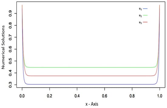
Figure 1. Graphical representation of numerical solutions for the case $\alpha {\mu }^2\le \gamma {ϵ}_i$.

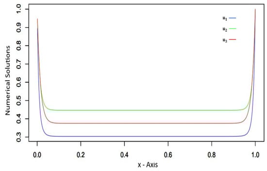
Figure 2. Graphical representation of numerical solutions for the case $\alpha {\mu }^2\ge \gamma {ϵ}_j$.

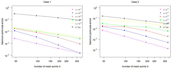
Figure 3. Graphical representation of maximum pointwise errors for different $\eta$ values for cases 1 and 2.

13. Conclusions

This paper presented a robust fitted mesh finite difference method for solving a system of two-parameter ‘n’ singularly perturbed differential equations of the convection–reaction–diffusion type. Using a piecewise uniform Shishkin mesh, our approach successfully captures the intricate behavior introduced by small perturbation parameters, which are typically challenging for conventional numerical methods. Our theoretical analysis establishes that the proposed scheme attains nearly first-order convergence in the maximum norm, uniformly with respect to both parameters. Numerical experiments confirm the method’s robustness and accuracy, demonstrating its capability to resolve boundary layers with precision across a system of equations. This work contributes to the numerical analysis of SPDEs by highlighting the importance of tailored methods for systems with small parameter effects. Future work can extend these results to enhance accuracy and efficiency in even more challenging scenarios of SPDEs.

References

- Bhatti, M.M.; Alamri, S.Z.; Ellahi, R.; Abdelsalam, S.I. Intra-uterine particle-fluid motion through a compliant asymmetric tapered channel with heat transfer. J. Therm. Anal. Calorim. 2021, 144, 2259–2267. [Google Scholar] [CrossRef]
- Glizer, V. Asymptotic analysis and solution of a finite-horizon H∞ control problem for singularly-perturbed linear systems with small state delay. J. Optim. Theory Appl. 2003, 117, 295–325. [Google Scholar] [CrossRef]
- Miller, J.J.H.; O’Riordan, E.; Shishkin, G.I. Fitted Numerical Methods for Singular Perturbation Problems; World Scientific: Singapore, 1996. [Google Scholar] [CrossRef]
- Doolan, E.P.; Miller, J.J.H.; Schilders, W.H.A. Uniform Numerical Methods for Problems with Initial and Boundary Layers; Boole Press: Dublin, Ireland, 1980. [Google Scholar]
- Cen, Z. Parameter-uniform finite difference scheme for a system of coupled singularly perturbed convection—diffusion equations. Int. J. Comput. Math. 2005, 82, 177–192. [Google Scholar] [CrossRef]
- Gracia, J.L.; O’Riordan, E.; Pickett, M.L. A parameter robust second order numerical method for a singularly perturbed two-parameter problem. Appl. Numer. Math. 2006, 56, 962–980. [Google Scholar] [CrossRef]
- Besova, M.; Kachalov, V. Axiomatic approach in the analytic theory of singular perturbations. Axioms 2020, 9, 9. [Google Scholar] [CrossRef]
- Liu, L.B.; Long, G.; Zhang, Y. Parameter uniform numerical method for a system of two coupled singularly perturbed parabolic convection-diffusion equations. Adv. Differ. Eq. 2018, 2018, 450. [Google Scholar] [CrossRef]
- Vishik, M.I.; Lyusternik, L.A. Regular degeneration and boundary layer for linear differential equations with small parameter. Russ. Math. Surv. 1957, 12, 3–122. [Google Scholar]
- O’Malley, R.E. Two-parameter singular perturbation problems for second-order equations. J. Math. Mech. 1967, 16, 1143–1164. [Google Scholar]
- O’Riordan, E.; Pickett, M.L.; Shishkin, G.I. Singularly perturbed problems modeling reaction-convection-diffusion processes. Comput. Methods Appl. Math. 2003, 3, 424–442. [Google Scholar] [CrossRef]
- Selvaraj, D.; Mathiyazhagan, J.P. A parameter uniform convergence for a system of two singularly perturbed initial value problems with different perturbation parameters and Robin initial conditions. Malaya J. Mat. 2021, 9, 498–505. [Google Scholar] [CrossRef] [PubMed]
- Kalaiselvan, S.S.; Miller, J.J.H.; Sigamani, V. A parameter uniform numerical method for a singularly perturbed two-parameter delay differential equation. Appl. Numer. Math. 2019, 145, 90–110. [Google Scholar] [CrossRef]
- Nagarajan, S. A parameter robust fitted mesh finite difference method for a system of two reaction-convection-diffusion equations. Appl. Numer. Math. 2022, 179, 87–104. [Google Scholar] [CrossRef]
- Arthur, J.; Chatzarakis, G.E.; Panetsos, S.L.; Mathiyazhagan, J.P. A robust-fitted-mesh-based finite difference approach for solving a system of singularly perturbed convection–diffusion delay differential equations with two parameters. Symmetry 2025, 17, 68. [Google Scholar] [CrossRef]
- Mathiyazhagan, P.; Sigamani, V.; Miller, J.J.H. Second order parameter-uniform convergence for a finite difference method for a singularly perturbed linear reaction-diffusion system. Math. Commun. 2010, 15, 587–612. [Google Scholar]
- Farrell, P.; Hegarty, A.; Miller, J.M.; O’Riordan, E.; Shishkin, G.I. Robust Computational Techniques for Boundary Layers, 1st ed.; Chapman and Hall/CRC: Boca Raton, FL, USA, 2000. [Google Scholar] [CrossRef]
Disclaimer/Publisher’s Note: The statements, opinions and data contained in all publications are solely those of the individual author(s) and contributor(s) and not of MDPI and/or the editor(s). MDPI and/or the editor(s) disclaim responsibility for any injury to people or property resulting from any ideas, methods, instructions or products referred to in the content. |
© 2025 by the authors. Licensee MDPI, Basel, Switzerland. This article is an open access article distributed under the terms and conditions of the Creative Commons Attribution (CC BY) license (https://creativecommons.org/licenses/by/4.0/).