On Quasi-Monotone Stochastic Variational Inequalities with Applications

Abstract

This paper studies an efficient method for solving stochastic optimization problems formulated as stochastic variational inequalities with a quasi-monotone operator, where the cost function extends the classical monotone and pseudomonotone operators. Our proposed method iterates an adaptive stepsize that adjusts automatically without linesearch and includes a momentum term to accelerate the convergence. Each iteration requires only a single projection onto the feasible set, ensuring low computational complexity. Under standard assumptions, the algorithm achieves almost sure convergence and a proven convergence rate. Furthermore, numerical experiments demonstrate its superior performance, accuracy, stability, and efficiency compared with existing stochastic approximation schemes. We also apply the method to problems such as stochastic network bandwidth allocation, stochastic complementarity problems, and the networked stochastic Nash–Cournot game, showing its strength and practical usefulness. The obtained result is an extension of existing works in the literature.

1. Introduction

We consider a stochastic optimization problem of the form:

$$\underset{x\in X}{min}F\left(x\right)=\mathbb{E}\left[f(x,\xi \left(\varpi \right))\right],$$

(1)

where x is the decision variable, X is a feasible subset of ${\mathbb{R}}^n$, $\xi :\mathsf{\Omega }\to \Xi$ is a random variable representing uncertainty, $f(x,\xi )$ is a random cost function, and $\mathbb{E}\left[f\right(x,\xi \left(\varpi \right)\left)\right]$ denotes its expectation. Problem (1) is known as a stochastic optimization (SO) problem.

Stochastic optimization provides a powerful framework for modeling and solving problems where randomness influences objectives or constraints. Such uncertainty is noticeable in real-world applications, including machine learning, where data are inherently noisy; finance, where markets fluctuate; engineering design, where measurements are imprecise; and energy systems, where renewable sources vary unpredictably (see, [1,2]). Unlike deterministic optimization, SO explicitly incorporates statistical variability into the modeling process, yielding solutions that are not only optimal in expectation but also robust under uncertainty. Its effectiveness lies in balancing exploration of the feasible region with exploitation of informative samples, which mitigates the risk of convergence to poor local minima in nonconvex or high-dimensional settings. Consequently, SO underpins many modern algorithms, such as stochastic gradient descent for deep learning, Monte Carlo-based optimization in engineering, and stochastic portfolio selection in finance.

In general, four classical approaches are used to solve problem (1): the stochastic gradient descent (SGD) method (see, e.g., [3]), the sample average approximation (SAA) [4], the stochastic approximation (SA) method [5], and evolutionary or Monte Carlo-based algorithms [6]. These methods have been extensively analyzed and successfully applied in diverse scientific and engineering domains. In this work, we focus on the SA framework, which is particularly effective when the expected value $\mathbb{E}\left[f\right(x,\xi \left)\right]$ is difficult or impossible to compute exactly. Our study connects SA methods to the theory of variational inequalities, providing a unified framework for optimization and equilibrium modeling under uncertainty.

The variational inequality problem (VIP), first introduced in [7], is a fundamental model that generalizes many problems in optimization, game theory, and economics. For a nonempty, closed, and convex set $X\subset {\mathbb{R}}^n$, the variational inequality problem (VIP) is expressed as follows:

$$\mathrm{F}\mathrm{i}\mathrm{n}\mathrm{d}x\in X\mathrm{such} \mathrm{that}⟨F\left(x\right),y-x⟩\ge 0,\forall y\in X,$$

(2)

where F is a nonlinear operator. Optimization problems correspond to VIP with $F=\nabla g$, where g is the objective function; Nash equilibrium conditions arise when F represents the vector of marginal payoffs; and traffic or network equilibrium problems appear when F models congestion effects [8]. Over the years, extensive studies (see, e.g., [9,10,11,12]) have focused on efficient numerical schemes and theoretical properties of deterministic VIP. However, in many practical situations, the operator F cannot be exactly computed due to noise or randomness. Examples include learning systems, where gradients are estimated from samples, financial models with stochastic returns, and network systems with uncertain demand. To address such cases, the notion of the stochastic variational inequality problem (SVIP) was developed in [5].

For clarity, assume that X is a nonempty, closed, and convex subset of ${\mathbb{R}}^n$, and let $(\mathsf{\Omega },\mathcal{F},\mathcal{P})$ denote a probability space. Consider a function $f:{\mathbb{R}}^n\times \Xi \to {\mathbb{R}}^n$ that is measurable with respect to the random variable $\xi :\mathsf{\Omega }\to \Xi$. The SVIP is formulated as

$$\begin{array}{c}\hfill \left\{\begin{array}{c}\mathrm{find}x\in X\mathrm{such} \mathrm{that}⟨F\left(x\right),y-x⟩\ge 0,\forall y\in X,\hfill \\ \mathrm{where} \mathrm{the} \mathrm{estimate}\hfill \\ F\left(x\right):=\mathbb{E}\left[f(x,\xi \left(\varpi \right))\right]={\int }_{\mathsf{\Omega }}f(x,\xi \left(\varpi \right))d\mathcal{P}\left(\varpi \right),\hfill \end{array}\right.\end{array}$$

(3)

and $\mathbb{E}$ denotes the expectation over $(\mathsf{\Omega },\mathcal{F},\mathcal{P})$. The SVIP generalizes the deterministic VIP by integrating stochastic effects into the equilibrium conditions and provides a rigorous model for decision-making under uncertainty. It encompasses diverse problems in stochastic optimization, energy markets, game theory, and transportation systems (see, e.g., [13,14]).

Related Works: Problem (3) has inspired substantial research activity. When $F\left(x\right)$ admits a closed-form expression, it reduces to the deterministic VIP (2), for which numerous efficient algorithms exist (see [11]). When $F\left(x\right)$ is not explicitly computable, two primary strategies are adopted: the sample average approximation (SAA) and the stochastic approximation (SA) approaches. In SAA, the expectation in (3) is replaced with an empirical average based on N independent samples:

$$F_N\left(x\right)={\displaystyle \frac{1}{N}}\sum _{i=1}^{N}f(x,{\xi }_i),$$

(4)

where $\left\{{\xi }_i\right\}$ are independent and identically distributed (i.i.d.) realizations of $\xi$ since the law of large numbers ensures that $F_N\left(x\right)\to F\left(x\right)$ almost surely as $N\to \infty$. Many recent studies analyze convergence properties of SAA and its applications to stochastic generalized equations [15], gap-function reformulations [16], and unconstrained settings [4,17,18,19]. In contrast, the SA framework solves (3) by updating iterates using sample-based gradients in an online fashion. The classical Robbins–Monro [5] procedure forms the basis for this approach. A seminal contribution by Jiang and Xu [14] proposed the single-projection SA algorithm:

$$x_{k+1}={\mathsf{\Pi }}_X(x_k-{\lambda }_{k}f(x_k,{\xi }_k)),\forall k\in {\mathbb{N}}_0,x_0\in X,$$

(5)

where ${\mathsf{\Pi }}_X$ denotes the Euclidean projection onto X, and the stepsize sequence $\left\{{\lambda }_k\right\}$ satisfies ${\sum }_{k=0}^{\infty }{\lambda }_k=\infty$ while ${\sum }_{k=0}^{\infty }{\lambda }_k^2<\infty$. Under strong monotonicity and Lipschitz continuity, they proved almost sure (a.s.) convergence to the unique solution of (3). Subsequent improvements have relaxed these assumptions or enhanced convergence properties. Yousefian et al. [20] introduced adaptive step-sizes for Cartesian SVIPs; Koshal et al. [21] proposed parallel and proximal-based methods; and [22] derived asymptotic feasibility and solution rates of $\mathcal{O}(1/k)$ and $\mathcal{O}(1/\sqrt{k})$, respectively, under the monotonicity assumption. To further weaken assumptions, Yang et al. [23] developed algorithms for pseudomonotone and Lipschitz continuous operators, achieving sublinear convergence and optimal oracle complexity.

Recent research has focused on improving algorithmic efficiency through the extragradient and subgradient extragradient (SEM) methods. The extragradient method, originally due to Korpelevich [24], has been successfully extended to the stochastic setting (see, e.g., [25,26]). A typical extragradient-type update reads:

$$\left\{\begin{array}{c}{y}_k={\mathsf{\Pi }}_X(x_k-{\gamma }_{k}f(x_k,{\xi }_k)),\hfill \\ x_{k+1}={\mathsf{\Pi }}_X(x_k-{\alpha }_{k}f(y_k,{\eta }_k)),\hfill \end{array}\right.$$

(6)

where ${\xi }_k$ and ${\eta }_k$ are independent sample batches. Although effective, this approach requires two projections per iteration, which can be computationally demanding for large-scale or structured feasible sets. To reduce this cost, subgradient extragradient variants [26,27,28,29] were proposed and analyzed for both deterministic and stochastic VIP, yielding promising results under monotonicity and Lipschitz continuity assumptions.

Furthermore, recent research works have introduced self-adaptive stepsize rules and inertial terms to accelerate convergence. In particular, Wang et al. [30] eliminated the need for linesearch-based parameter tuning while maintaining convergence for pseudomonotone operators and adopted self-adaptive strategy to analysis approximate solution to SA. Liu and Qin [31] later incorporated Polyak’s inertial extrapolation [32] (see, also [33,34,35,36,37]) into stochastic extragradient frameworks, achieving almost sure convergence and improved complexity bounds, though still requiring linesearch conditions.

Motivation and Contribution: Despite these advances, most existing SA-based algorithms rely on strong or pseudomonotone assumptions, limiting their applicability to broader problem classes. Moreover, modern schemes often require multiple projections, sensitive parameter tuning, or complex linesearch procedures, which hinder scalability. Motivated by these challenges and the works in [23,27,30,31,32,38,39], we ask the following fundamental question:

Question: Can we design a robust iterative scheme for solving the SVIP (3) that combines self-adaptive step-sizes, stochastic subgradient extragradient techniques, and inertial acceleration for a quasi-monotone operator within the SA framework while ensuring almost sure and convergence rate are guarantees?

The principal objective of this study is to provide an affirmative answer to this question.

Organization of the Paper: Section 2 presents preliminary definitions and essential lemmas. Section 3 introduces the proposed algorithm and underlying assumptions. Section 4 contains the main convergence analysis and proofs. Numerical results and practical applications are presented in Section 5, followed by concluding remarks in Section 6.

2. Preliminaries

In this section, we formally state some basic terminologies that are essential in this work. For any vectors $x,y\in {\mathbb{R}}^n,⟨x,y⟩$ is the standard inner product, $\parallel x\parallel =\sqrt{⟨x,y⟩}$ is the Euclidean norm. Given $\xi$ a random variable and $\sigma -$ algebra $\mathcal{F},$ the notations $\mathbb{E}\left[\xi \right],\mathbb{E}\left[\xi \right|\mathcal{F}],V(\xi )$ and $V\left(\xi \right|\mathcal{F})$ denote the expectation of $\xi$, conditional expectation of $\xi$ with respect to $\mathcal{F}$, the variance of $\xi$ and the conditional variance of $\xi$ with respect to $\mathcal{F}$. For $p\ge {1,\left|\xi \right|}_p:\sqrt[p]{\mathbb{E}\left[\xi {|}^p\right]}$ is the $L_p$ norm of $\xi$ and ${\left|\xi \right|\mathcal{F}|}_p:=\sqrt[p]{\mathbb{E}\left[\xi {|}^p\right|\mathcal{F}]}$ is the $L_p$ norm of $\xi$ conditional to $\mathcal{F}$. The $\sigma -$ algebra generated by the random variable ${\left\{{\xi }_k\right\}}_{i=1}^k$ is denoted by $\sigma ({\xi }_1,\dots ,{\xi }_k).$ Also, $\mathbb{E}[.|{\xi }_1,\dots ,{\xi }_k]:=\mathbb{E}[.|\sigma ({\xi }_1,\dots ,{\xi }_k)]$. We say that a random variable $\xi$ is $\mathcal{F}$-measurable. We write $\xi \perp \perp \mathcal{F}$ to mean that $\xi$ is independent of the $\sigma$-algebra $\mathcal{F}$. The set of natural number is denoted by $\mathbb{N}$. Let $x\in {\mathbb{R}}^n,$ there exists a unique element $z\in X,$ denoted by ${\mathsf{\Pi }}_X\left(x\right),$ such that $\parallel z-x\parallel ={inf}_{y\in X}\parallel y-z\parallel .$ The mapping ${\mathsf{\Pi }}_X:{\mathbb{R}}^n\to X$ is called a projection from ${\mathbb{R}}^n$ onto $X.$ To quantify the inaccuracy in the stochastic evaluation of (3), introduce the error term

$$\epsilon (x,\xi ):=f(x,\xi )-F\left(x\right),x\in {\mathbb{R}}^n,\xi \in \Xi .$$

For any exponent $p\in [2,\infty )$, we associate with this error the p-moment function

$${\sigma }_p\left(x\right)={\left({\mathbb{E}\parallel \epsilon (x,\xi )\parallel }^p\right)}^{1/p},$$

which serves as an indicator of how accurately a stochastic approximation method captures the underlying operator.

We give below a fundamental definition regarding the cost function.

Definition 1.

The mapping T on X is called:

(i) 

strongly monotone if, there exists a constant $\mu >0$ such that for all

$$x,y\in X,⟨Tx-Ty,x-y⟩\ge {\mu \parallel x-y\parallel }^2;$$

(ii) 

monotone if, for all $x,y\in X,⟨Tx-Ty,x-y⟩\ge 0;$

(iii) 

pseudomonotone if, for all $x,y\in X,⟨Ty,x-y⟩\ge 0\Rightarrow ⟨Tx,x-y⟩\ge 0;$

(iv) 

quasi-monotone if, for all $x,y\in X,⟨Ty,x-y⟩>0\Rightarrow ⟨Tx,x-y⟩\ge 0.$

Remark 1.

We obtain from Definition 1 that $\left(1\right)\Rightarrow \left(2\right)\Rightarrow \left(3\right)\Rightarrow \left(4\right)$, but the converse of these statements is not true in general.

The following Lemmas are very important in our work.

Lemma 1

(Lemma 2.1, [30]). Let ${\mathsf{\Pi }}_X$ be a projection from ${\mathbb{R}}^n$ onto $X.$ Then,

(i) 

$\parallel {\mathsf{\Pi }}_X{\left(x\right)-z\parallel }^2\le {\parallel x-z\parallel }^2-{\parallel {\mathsf{\Pi }}_X\left(x\right)-x\parallel }^2,\forall x\in {\mathbb{R}}^n$ and $z\in X.$

(ii) 

$2⟨v,u-z⟩\le {\parallel y-z\parallel }^2{-\parallel u-z\parallel }^2-{\parallel u-y\parallel }^2.$

(iii) 

$z={\mathsf{\Pi }}_X\left(x\right)$ if and only if $⟨x-z,z-y⟩\ge 0,\forall y\in X.$

(iv) 

Let $\mathsf{\Gamma }\ne \varnothing .$ Then, $x^{\ast }\in \mathsf{\Gamma }\iff x^{\ast }={\mathsf{\Pi }}_X(x^{\ast }-\alpha F\left(x^{\ast }\right))$ for all $\alpha$ strictly positive.

Let $\overline{x},\begin{array}{c}\hfill v\end{array}\in {\mathbb{R}}^n$ with $v\ne 0$ and consider $T_k=\{x\in {\mathbb{R}}^n:⟨v,,x-\overline{x}⟩\le 0\}.$ For any $y\in {\mathbb{R}}^n,$ the projection ${\mathsf{\Pi }}_{T_k}\left(x\right)$ is given by

$${\mathsf{\Pi }}_{T_k}\left(y\right)=y-max\left\{0,{\displaystyle \frac{⟨v,y-\overline{x}⟩}{{\left|v\right|}^2}}\right\}v.$$

(7)

Observe that (7) provides a direct formula for computing the projection of an arbitrary point onto a half-space.

Lemma 2

([40]). For any point $x\in {\mathbb{R}}^n$ and any parameter $\beta >0,$ the following bounds are satisfied:

$$min\{1,\beta \}{r}_1\left(x\right)\le r_{\beta }\left(x\right)\le max\{1,\beta \}{r}_1\left(x\right)$$

where $r_{\beta }\left(x\right)=\parallel x-{\mathsf{\Pi }}_X(x-\beta F\left(x\right))\parallel .$

Assumption 1

The following assumptions shall be considered:

(A) 

The solution set $\mathsf{\Gamma }\ne \varnothing .$

(B) 

(i) For all $x,y\in {\mathbb{R}}^n$ and almost every $\varpi \in \mathsf{\Gamma },$

$$\parallel f(x,\xi (\varpi \left)\right)-f(y,\xi (\varpi \left)\right)\parallel \le L\left(\xi \right(\varpi \left)\right)\parallel x-y\parallel ,$$

    where $\mathcal{L}:\Xi \to {\mathbb{R}}^{+}$ is a measurable function such that $\mathcal{L}\left(\xi \right(\varpi \left)\right)\ge 1$ for almost $\varpi \in \mathsf{\Gamma }.$

(ii) There exists $a\in {\mathbb{R}}^n$ and $p\ge 2$ such that $\mathbb{E}[\parallel f(a,\xi ){\parallel }^p]<\infty$ and $\mathbb{E}\left[\mathcal{L}{\left(\xi \right)}^p\right]<\infty .$

(C) 

The mapping F is quasi-monotone.

(D) 

Let ${\eta }_k\in (0,1)$ and $\left\{{\delta }_k\right\}$ a positive sequence such that ${lim}_{k\to \infty }{\eta }_k=0$ and ${\sum }_{k=0}^{\infty }{\eta }_k=+\infty .$ Furthermore, ${\displaystyle \frac{{\delta }_k}{{\eta }_k}}\to 0$ as $k\to \infty .$

Lemma 3

([41]). Under Assumption 1, the operators F and ${\sigma }_q(·)$ are Lipschitz continuous on ${\mathbb{R}}^n$ with constants L and $L_q$, respectively. This holds for every $q\in [p,2p]$, where p is the exponent specified in Assumption 1. Moreover, the constants satisfy $L=\mathbb{E}\left[\mathcal{L}\right(\xi \left)\right]$ and $L_q=\sqrt[q]{\mathbb{E}\left[\mathcal{L}{\left(\xi \right)}^q\right]}+L.$ Let $\xi ={\left\{{\xi }_j\right\}}_{j=1}^N$ denote an i.i.d. collection drawn from Ξ, and define

$$\begin{array}{c}\hfill G(x,\xi )={\displaystyle \frac{1}{N}}\sum _{j=1}^{N}f(x,{\xi }_j)and\overline{\epsilon }(x,\xi )={\displaystyle \frac{1}{N}}\sum _{j=1}^N\epsilon (x,{\xi }_j).\end{array}$$

Lemma 4

([41]). Suppose that Assumption 1 holds. Then, for any $q\in [p,2p]$ with p from Assumption 1, there exists a constant $C_q>0$ such that for any $x\in {\mathbb{R}}^n,x^{\ast }\in \mathsf{\Gamma }$,

$$\begin{array}{c}\hfill |\overline{\epsilon }{(x,\xi )|}_q\le C_q{\displaystyle \frac{{\sigma }_q\left(x^{\ast }\right)+L_q\parallel x-x^{\ast }\parallel }{\sqrt{N}}}.\end{array}$$

Lemma 5

([41]). Assume that Assumption 1 holds and $\mathsf{\Gamma }\ne \varnothing .$ Let ${\lambda }_N:\Xi \to [0,\lambda ]$ be a random variable for some $0<\lambda \le 1.$ Define $z(x,{\lambda }_N,\xi )={\mathsf{\Pi }}_X(x-{\lambda }_{N}G(x,\xi )).$ Then, for any $p\ge 2,$ there exist positive constants ${\left\{c_i\right\}}_{i=1}^4$ (depending on $n,p,and\lambda$) such that

$$\begin{array}{c}\hfill |\overline{\epsilon }(z(x,{\lambda }_N,\xi ),\xi ){|}_p\ge {\displaystyle \frac{c_1{\sigma }_{2p}\left(x^{\ast }\right)+{\overline{L}}_{2p}\parallel x-x^{\ast }\parallel }{\sqrt{N}}},\forall x\in {\mathbb{R}}^n,\forall x^{\ast }\in \mathsf{\Gamma },\end{array}$$

(8)

where ${\overline{L}}_{2p}=c_2{L}_2+c_3{L}_p+c_4{L}_{2p},c_1>C_p$ and ${\sigma }_{2p}\left(x^{\ast }\right)\ge {\sigma }_p\left(x^{\ast }\right).$

Lemma 6

([42]). Let ${\left\{V_k\right\}}_{k\ge 1},{\left\{{\delta }_k\right\}}_{k\ge 1},{\left\{{\eta }_k\right\}}_{k\ge 1}$ and ${\left\{{\beta }_k\right\}}_{k\ge 1}$ denote sequences of nonnegative random variables adapted to the filtration ${\left\{{\mathsf{\Theta }}_k\right\}}_{k\ge 1}$. Suppose that, almost surely, ${\sum }_{k=1}^{\infty }{\delta }_k<\infty$ and ${\sum }_{k=1}^{\infty }{\mathsf{\Theta }}_k<\infty$, and that

$$\begin{array}{c}\hfill [V_{k+1}\mid {\mathsf{\Theta }}_k]\le (1+{\delta }_k)V_k-{\eta }_k+{\beta }_k,\forall k\in \mathbb{N}.\end{array}$$

Then, with probability one, the sequence $\left\{V_k\right\}$ converges and ${\sum }_{k=1}^{\infty }{\eta }_k<\infty .$

3. Proposed Algorithm

Remark 2.

We highlight the benefits Algorithm 1 as follow:

1. 

In the Step 1 of the proposed algorithm, we incorporate the inertial term ${\theta }_k(x_k-x_{k-1}),$ also called momentum-based method inspired by Nesterov acceleration and Polyak’s heavy-ball method. It promises faster convergence rates, variance reduction, better stability for ill-conditioned problems, and improved practical performance. It is obvious that without inertia, SA can become stuck in flat regions or plateaus caused by noise. In stochastic games, inertial SA often requires fewer iterations to achieve a desired accuracy. These facts underscore the need for adopting it in the algorithm, and it is an improvement over [5,21,23,25,27,28,30,39,41].

2. 

The algorithm involves the subgradient extragradient (SEG) method, which involves one projection onto the feasible set. It handles non-smooth problems, improves feasibility maintenance, which ensures all iterates remain feasible, a key requirement in constrained stochastic optimization problems. It is, therefore, preferable to those algorithms that involve two projections onto the feasible set per iteration. Hence, it contributes positively to the literature when compared with works in [5,14,15,20,21,22,25,27,33,41,42].

3. 

Since the SA-based algorithm is very sensitive to the stepsize or the step-length, we consider a self-adaptive stepsize that adjusts dynamically, ensuring robustness across problem scales and conditions. In fact, self-adaptive stepsize in SA accelerates convergence, reduces sensitivity to noise, eliminates heavy manual turning, ensures stability, and equally improves efficiency near the solution. Unlike Armijo linesearch methods that consume a large amount of time, thereby affecting the performance of iterative algorithms (see, e.g., [4,13,14,15,17,21,31,33,40,41,42,42]) and cited references contained therein.

4. 

It is known that real-world stochastic systems often have non-symmetric or partially monotone structures. This necessitated the very essence of considering a quasi-monotone operator, which is weaker, so that the proposed scheme can handle nonlinear, asymmetric, or discontinuous mappings more realistically. It is important to note that quasi-monotone operators avoid the need for projection correctness or strong-regularization techniques required for non-monotone problems. To this end, Algorithm 1 offers greater modeling flexibility, wider applicability, reduced assumptions for convergence, and lower computational cost compared to strict monotonicity, monotonicity, and pseudo-monotonicity commonly found in the literature. Therefore, our scheme improves many already announced results in this research direction.

Algorithm 1 Inertial Self-Adaptive Subgradient Extragradient Algorithm

Step 0: Select $x_0,x_1\in {\mathbb{R}}^n,{\alpha }_0>0.$ Take $\theta \in [0,1),{\epsilon }_0\in [0,1),\forall k\in {\mathbb{N}}_0,\mu \in (0,{\displaystyle \frac{1}{2}}).$ Take the sample rate ${\left\{N_k\right\}}_{k\ge 0}$ with ${\sum }_{k=0}^{\infty }{\displaystyle \frac{1}{\sqrt{N_k}}}<\infty .$ Set $k=0.$ Step 1: Given the current iterates $x_k,x_{k-1},(k\ge 0),$ construct the inertial term as follows: $$w_k=x_k+{\theta }_k(x_k-x_{k-1}),$$ (9) where $${\theta }_k=\left\{\begin{array}{c}min\{{\displaystyle \frac{{\delta }_k}{\parallel x_k-x_{k-1}\parallel }},\theta \}if{x}_k\ne x_{k-1},\hfill \\ \theta ,otherwise.\hfill \end{array}\right.$$ Step 2: Draw an i.i.d. sample ${\xi }_k={\left\{{\xi }_j^k\right\}}_{j=1}^{N_k}$ from $\Xi$ and compute $$y_k={\mathsf{\Pi }}_X(w_k-{\alpha }_{k}G(w_k,{\xi }_k)),$$ (10) where $G(w_k,{\xi }_k)={\displaystyle \frac{1}{N_k}}{\sum }_{j=1}^{N_k}f(w_k,{\xi }_j^k).$ If $w_k=x_k=y_k,$ then stop, $w_k\in \mathsf{\Gamma };$ otherwise, go to the next step. Step 3: Consider a constructible set $T_k=\{x\in {\mathbf{R}}^n:⟨w_k-{\alpha }_{k}G(w_k,{\xi }_k)-y_k,x-y_k⟩\le 0\}$ and calculate $$x_{k+1}={\mathsf{\Pi }}_{T_k}(w_k-{\alpha }_{k}G(y_k,{\xi }_k)),$$ (11) where $G(y_k,{\xi }_k)={\displaystyle \frac{1}{N_k}}{\sum }_{j=1}^{N_k}f(y_k,{\xi }_j^k),$ $${\alpha }_{k+1}=\left\{\begin{array}{c}min\{{\alpha }_k,{\displaystyle \frac{\mu \parallel y_k-w_k\parallel }{\parallel G(w_k,{\xi }_k)-G(y_k,{\xi }_k)\parallel }}\},ifG(w_k,{\xi }_k)\ne G(y_k,{\xi }_k),\hfill \\ {\alpha }_k,\mathrm{otherwise}.\hfill \end{array}\right.$$ (12) Set $k:=k+1$ and go back to Step 1.

4. Convergence Analysis

In this section, we present the technical proofs for two convergence analyses of the proposed Algorithm 1: almost sure convergence and the rate of convergence. The former establishes pathwise convergence without quantifying the speed of approach, whereas the latter measures the convergence speed rather than probabilistic pathwise certainty. We begin with the proof of almost surely convergence.

4.1. Almost Surely Convergence

Remark 3.   1.  Our investigation of the proposed method will be based on filtration ${\mathcal{F}}_k$.

$${\mathcal{F}}_0=\sigma \left(x_0\right)and\mathcal{F}(x_0,{\xi }_0,\dots ,{\xi }_{k-1})\forall k\in \mathbb{N}.$$

So,

$${\mathcal{F}}_0=\sigma \left(x_0\right),{\mathcal{F}}_1=\sigma (x_0,{\xi }_0),{\mathcal{F}}_2=\sigma (x_0,{\xi }_0,{\xi }_1),\dots$$

Increasingly, ${\mathcal{F}}_k=\sigma (x_0,{\xi }_0,\dots ,{\xi }_{k-1})$ and ${\mathcal{F}}_{k+1}=\sigma (x_0,{\xi }_0,\dots ,{\xi }_k).$ We see clearly that adding ${\xi }_k$ provides more information, so ${\mathcal{F}}_k\subset {\mathcal{F}}_{k+1}.$ Since $x_k$ is a measurable function of $(x_0,{\xi }_0,\dots ,{\xi }_{k-1}).$ It follows that $x_k\subset {\mathcal{F}}_k.$

2. 

From the Algorithm 1, and (7) it follows that for any given $x\in {\mathbb{R}}^n,$

$$\begin{array}{c}\hfill x_{k+1}=x-max\left\{0,{\displaystyle \frac{⟨w_k-{\alpha }_{k}G(w_k,{\xi }_k)-y_k,x-y_k⟩}{\parallel w_k-{\alpha }_{k}G(w_k,{\xi }_k)-y_k{\parallel }^2}}\right\}(w_k-{\alpha }_{k}G(w_k,{\xi }_k)-y_k),\end{array}$$

provided that $w_k-{\alpha }_{k}G(w_k,{\xi }_k)-y_k\ne 0.$ This is one of striking advantage of Algorithm 1. Its execution is merely a single projection onto $X,$ creating efficiency and smooth running of the scheme.

3. 

Let $X\subset {\mathbb{R}}^n.$ From Algorithm 1, Step 2, we know that $y_k={\mathsf{\Pi }}_X(w_k-{\alpha }_{k}G(w_k,{\xi }_k))$ i.e., $y_k$ is the projection of $(w_k-{\alpha }_{k}G(w_k,{\xi }_k)$ onto $X.$ Using projection property, we understand that

$$\begin{array}{c}\hfill ⟨z-y_k,x-y_k⟩\le 0,\forall x\in X,\end{array}$$

where z is the point being projected, i.e., $z=(w_k-{\alpha }_{k}G(w_k,{\xi }_k).$ Using the definition of $T_k$ from the algorithm, we understand that for all

$$x\in X,T_k=\{x\in {\mathbb{R}}^n:⟨w_k-{\alpha }_{k}G(w_k,{\xi }_k)-y_k,x-y_k⟩\le 0\}.$$

So, $X\subset T_k.$

4. 

In view of (5), we define ${\epsilon }_1^k=G(w_k,{\xi }_k)-F\left(w_k\right)$ and ${\epsilon }_2^k=G(y_k,{\xi }_k)-F\left(y_k\right)$ the oracle errors for all $k\in \mathbb{N}.$ If $w_k=x_k=y_k$ for some $k\in {\mathbb{N}}_0,$ then $w_k\in \mathsf{\Gamma }.$

Indeed, assume that $w_k=x_k=y_k$ for some positive $k.$ We know from Lemma 1 (i) that

$$\begin{array}{ccc}\hfill \parallel y_k{-x\parallel }^2& =& \parallel {\mathsf{\Pi }}_X(w_k-{\alpha }_{k}G(w_k,{\xi }_k)){-x\parallel }^2\hfill \\ & \le & \parallel w_k-{\alpha }_{k}G(w_k,{\xi }_k){-x\parallel }^2-{\parallel w_k-{\alpha }_{k}G(w_k,{\xi }_k)-y_k\parallel }^2\hfill \\ & =& \parallel w_k-{\alpha }_{k}G(w_k,{\xi }_k){-x\parallel }^2-{\alpha }_k^2{\parallel G(w_k,{\xi }_k)\parallel }^2\hfill \\ & =& \parallel y_k{-x\parallel }^2-2{\alpha }_k⟨w_k-x,G(w_k,{\xi }_k)⟩\hfill \\ & =& \parallel y_k{-x\parallel }^2-2{\alpha }_k⟨w_k-x,F\left(w_k\right)⟩-2{\alpha }_k⟨w_k-x,{\epsilon }_1^k⟩.\hfill \end{array}$$

(13)

Noting that ${\alpha }_k>0,$ we quickly have that

$$\begin{array}{c}\hfill ⟨w_k-x,F\left(w_k\right)⟩+⟨w_k-x,{\epsilon }_1^k⟩\le 0,\forall x\in X.\end{array}$$

Indeed, for all $x\in X,\{{\lambda }_k⟨{\epsilon }_1^k,w_k-x⟩,{\mathcal{F}}_k\}$ defines a martingale difference, i.e., $\mathbb{E}\left[{\lambda }_k⟨{\epsilon }_1^k,w_k-x⟩\right|{\mathcal{F}}_k]=0.$ This follows from the fact that since $w_k\in {\mathcal{F}}_k$ and ${\xi }_k\perp \perp {\mathcal{F}}_k,$ we understand that

$$\begin{array}{ccc}\hfill \mathbb{E}\left[{\epsilon }_1^k\right|{\mathcal{F}}_k]& =& \mathbb{E}\left[G(w_k,{\xi }_k)\right|{\mathcal{F}}_k]-F\left(w_k\right)\hfill \\ & =& \mathbb{E}\left[G(x,{\xi }_k)\right]{|}_{x=w_k}-F\left(w_k\right)\hfill \\ & =& 0.\hfill \end{array}$$

(14)

Taking $\mathbb{E}[.|{\mathcal{F}}_k],$ in (13)

$$⟨w_k-x,F\left(w_k\right)⟩+\mathbb{E}\left[⟨w_k-x,{\epsilon }_1^k⟩\right|{\mathcal{F}}_k]=⟨w_k-x,F\left(w_k\right)⟩<0,\forall x\in X.$$

Therefore, $w_k\in \mathsf{\Gamma }.$

We shall break our main theorem into Lemmas.

Lemma 7.

The limit of $\left\{{\alpha }_k\right\}$ a.s. exists. Let ${lim}_{k\to \infty }{\alpha }_k=\alpha$ as $k\to \infty .$ Then, $\alpha \ge min\{{\alpha }_0,{\displaystyle \frac{\mu }{L}}\},$ where $L=\mathbb{E}\left[\mathcal{L}\right(\xi \left)\right].$

Proof. 

By the definition of ${\lambda }_{k+1}$ in the algorithm, we obtain

$${\lambda }_{k+1}=min\left\{{\lambda }_k,{\displaystyle \frac{\mu \parallel y_k-x_k\parallel }{\parallel G(x_k,{\xi }_k)-G(y_k,{\xi }_k)\parallel }}\right\}\le {\lambda }_k,$$

(15)

which shows that the sequence $\left\{{\lambda }_k\right\}$ is monotone nonincreasing, and moreover ${\lambda }_k>0$ for every k.

Hence $\left\{{\lambda }_k\right\}$ is bounded below by 0 and thus convergent almost surely to a finite limit $\lambda :={lim}_{k\to \infty }{\lambda }_k\ge 0$.

Now, define

$$A_k:={\displaystyle \frac{1}{N_k}}\sum _{j=1}^{N_k}L\left({\xi }_j^k\right),$$

where $L\left(\xi \right)$ is the random Lipschitz modulus from Assumption 1 and ${\left\{{\xi }_j^k\right\}}_{j=1}^{N_k}$ are the sampled random variables at iteration k.

The Lipschitz-type bound implies that

$$\parallel G(x_k,{\xi }_k)-G(y_k,{\xi }_k)\parallel \le A_k\parallel x_k-y_k\parallel .$$

If $G(x_k,{\xi }_k)\ne G(y_k,{\xi }_k)$, then

$${\displaystyle \frac{\mu \parallel y_k-x_k\parallel }{\parallel G(x_k,{\xi }_k)-G(y_k,{\xi }_k)\parallel }}\ge {\displaystyle \frac{\mu }{A_k}}.$$

(16)

Thus,

$${\lambda }_{k+1}\ge min\{{\lambda }_k,\frac{\mu }{A_k}\}.$$

Iterating this inequality gives

$${\lambda }_{k+1}\ge min\left\{{\lambda }_0,{\displaystyle \frac{\mu }{A_0}},{\displaystyle \frac{\mu }{A_1}},\dots ,{\displaystyle \frac{\mu }{A_k}}\right\}.$$

(17)

Assume, for contradiction, that

$$\lambda <min\{{\lambda }_0,\frac{\mu }{L}\}.$$

Choose $\eta$ such that

$$\lambda <\eta <min\{{\lambda }_0,\frac{\mu }{L}\}.$$

Since ${\lambda }_k\to \lambda$ almost surely as $k\to \infty ,$ there exists (a.s.) $k_0$ such that for all $k>k_0$, ${\lambda }_{k+1}<\eta$. By definition of ${\lambda }_{k+1}$, whenever ${\lambda }_{k+1}<\eta$ we must have

$${\displaystyle \frac{\mu }{A_k}}<\eta ⟹A_k>{\displaystyle \frac{\mu }{\eta }}.$$

Hence, for all large k,

$$\mathbb{E}\left[A_k\right]>{\displaystyle \frac{\mu }{\eta }}.$$

But $\mathbb{E}\left[A_k\right]=\mathbb{E}\left[{\displaystyle \frac{1}{N_k}}{\sum }_{j=1}^{N_k}L\left({\xi }_j^k\right)\right]=\mathbb{E}\left[L\left(\xi \right)\right]=L,$ since the ${\xi }_j^k$ are i.i.d. Therefore $L>\frac{\mu }{\eta }$, implying $\eta >\frac{\mu }{L}$, which contradicts $\eta <\frac{\mu }{L}$.

Thus, the assumption is false, and we conclude that

$$\lambda \ge min\{{\lambda }_0,\frac{\mu }{L}\}.$$

□

Remark 4.

The expectation step is justified because $A_k$ is the empirical mean of i.i.d. random variables $L\left({\xi }_j^k\right)$, so that $\mathbb{E}\left[A_k\right]=\mathbb{E}\left[L\left(\xi \right)\right]=L$. The contradiction argument uses that if $A_k>\mu /\eta$ for all large k, then $L=\mathbb{E}\left[A_k\right]\ge {\displaystyle \frac{\mu }{\eta }}$, contradicting $\eta <\mu /L$. This gives a transparent probabilistic justification for the bound.

The following Lemma will be needed in the sequel.

Lemma 8.

For any $x^{\ast }\in \mathsf{\Gamma }$, the following estimate holds almost surely:

$$\begin{array}{ccc}\hfill \parallel x_{k+1}-x^{\ast }{\parallel }^2& \le & \parallel x_k-x^{\ast }{\parallel }^2-(1-{\tau }_k)\left[\parallel x_{k+1}{-yk\parallel }^2+{\parallel y_k-w_k\parallel }^2\right]\hfill \\ & & +2{\alpha }_0\parallel {\epsilon }_2^k\parallel \parallel y_k-x^{\ast }\parallel +3M_2{\eta }_k,\forall k\in {\mathbb{N}}_0,\hfill \end{array}$$

(18)

where ${\tau }_k={\displaystyle \frac{2\mu {\alpha }_k}{{\alpha }_{k+1}}}.$

Proof. 

Recall from the inertial term step that $w_k=x_k+{\theta }_k(x_k-x_{k-1})$ and for any $x^{\ast }\in \mathsf{\Gamma },$ using definition of $\left\{w_k\right\}$ and $\left\{{\theta }_k\right\},$ we obtain

$${\theta }_k\parallel x_k-x_{k-1}\parallel \le {\delta }_k,\forall n\ge 1.$$

Hence,

$${\displaystyle \frac{{\theta }_k}{{\eta }_k}}\parallel x_k-x_{k-1}\parallel \le {\displaystyle \frac{{\delta }_k}{{\eta }_k}}\to 0asn\to \infty .$$

Therefore, there exists $M_1>0$ such that

$${\displaystyle \frac{{\theta }_k}{{\eta }_k}}\parallel x_k-x_{k-1}\parallel \le M_1,k\ge 1.$$

$$\begin{array}{ccc}\hfill \parallel w_k-x^{\ast }{\parallel }^2& =& \parallel x_k-x^{\ast }+{\theta }_k(x_k-x_{k-1}){\parallel }^2\hfill \\ & \le & \parallel x_k-x^{\ast }{\parallel }^2+{\theta }_k^2\parallel x_k-x_{k-1}{\parallel }^2+2{\theta }_k\parallel x_k-x^{\ast }\parallel \parallel x_k-x_{k-1}\parallel \hfill \\ & =& \parallel x_k-x^{\ast }{\parallel }^2+{\theta }_k\parallel (x_k-x_{k-1})\parallel \left[2\parallel x_k-x^{\ast }\parallel +{\theta }_k\parallel x_k-x_{k-1}\parallel \right]\hfill \\ & \le & \parallel x_k-x^{\ast }{\parallel }^2+3{\theta }_k\parallel x_k-x_{k-1}\parallel M_0\hfill \\ & =& \parallel x_k-x^{\ast }{\parallel }^2+3M_0{\eta }_k{\displaystyle \frac{{\theta }_k}{{\eta }_k}}\parallel x_k-x_{k-1}\parallel \hfill \\ & \le & \parallel x_k-x^{\ast }{\parallel }^2+3M_1{M}_0{\eta }_k\hfill \\ & =& \parallel x_k-x^{\ast }{\parallel }^2+3M_2{\eta }_k,\hfill \end{array}$$

(19)

for some $0<M_2=M_0{M}_1.$

In view of the fact that $\mathsf{\Gamma }\subset X\subset T_k$ holds for all $k\in {\mathbb{N}}_0,$ and for each $x^{\ast }\in \mathsf{\Gamma }$ with Lemma 1 (ii), (20) and for any $w_k\in X,$ we understand that

$$2{\alpha }_k⟨G(y_k,{\xi }_k),x_{k+1}-x^{\ast }⟩\le \parallel w_k-x^{\ast }{\parallel }^2-\parallel x_{k+1}-x^{\ast }{\parallel }^2-{\parallel x_{k+1}-w_k\parallel }^2.$$

That is,

$$\begin{array}{ccc}\hfill \parallel x_{k+1}-x^{\ast }{\parallel }^2& \le & \parallel w_k-x^{\ast }{\parallel }^2-{\parallel x_{k+1}-w_k\parallel }^2+2{\alpha }_k⟨G(y_k,{\xi }_k),x^{\ast }-x_{k+1}⟩\hfill \\ & =& \parallel w_k-x^{\ast }{\parallel }^2-{\parallel x_{k+1}-y_k+y_k-w_k\parallel }^2+2{\alpha }_k⟨G(y_k,{\xi }_k),x^{\ast }-x_{k+1}⟩\hfill \\ & =& \parallel w_k-x^{\ast }{\parallel }^2-\left[\parallel x_{k+1}-y_k{\parallel }^2+{\parallel y_k-w_k\parallel }^2++2⟨x_{k+1}-y_k,y_k-w_k⟩\right]\hfill \\ & & +2{\alpha }_k⟨G(y_k,{\xi }_k),x^{\ast }-x_{k+1}⟩\hfill \\ & \le & \parallel x_k-x^{\ast }{\parallel }^2-\left(\parallel x_{k+1}-w_k{\parallel }^2+{\parallel y_k-w_k\parallel }^2\right)\hfill \\ & & +2{\alpha }_k⟨G(y_k,{\xi }_k),x^{\ast }-y_k⟩\hfill \\ & & +2⟨x_{k+1}-y_k,w_k-y_k-{\alpha }_{k}G(y_k,{\xi }_k)⟩+3M_2{\eta }_k.\hfill \end{array}$$

(20)

Since $x_{k+1}$ lies in $T_k,$ it follows that

$$\begin{array}{c}\hfill ⟨x_{k+1}-y_k,w_k-y_k-{\alpha }_{k}G(w_k,{\xi }_k)⟩\le 0,\end{array}$$

which further implies that

$$\begin{array}{c}\hfill ⟨x_{k+1}-y_k,w_k-y_k-{\alpha }_{k}G(y_k,{\xi }_k)⟩\le {\alpha }_k⟨x_{k+1}-y_k,G(w_k,{\xi }_k)-G(y_k,{\xi }_k)⟩,\forall k\in {\mathbb{N}}_0.\end{array}$$

(21)

Indeed, we know that

$$w_k-y_k-{\alpha }_{k}G(w_k,{\xi }_k)=(w_k-y_k-{\alpha }_k)G(y_k,{\xi }_k)-{\alpha }_k\left(G(w_k,{\xi }_k)-G(y_k,{\xi }_k)\right).$$

Taking inner product with $x_{k+1}-y_k,$ using linearity gives

$$\begin{array}{ccc}\hfill 0& \ge & ⟨x_{k+1}-y_k,w_k-y_k-{\alpha }_{k}G(w_k,{\xi }_k)⟩\hfill \\ & =& ⟨x_{k+1}-y_k,w_k-y_k-{\alpha }_{k}G(w_k,{\xi }_k)⟩-{\alpha }_k⟨x_{k+1}-y_k,G(w_k,{\xi }_k)-G(y_k,{\xi }_k)⟩.\hfill \end{array}$$

Re-arranging the above inequality, we obtain (21). Furthermore, applying Cauchy–Schwartz inequality, utilizing the definition of ${\alpha }_{k+1}$ given in Algorithm 1, one obtains

$$\begin{array}{ccc}\hfill 2{\alpha }_k⟨x_{k+1}-y_k,G(w_k,{\xi }_k)-G(y_k,{\xi }_k)⟩& \le & 2{\alpha }_k\parallel x_{k+1}-y_k\parallel \parallel G(w_k,{\xi }_k)-G(y_k,{\xi }_k)\parallel \hfill \\ & \le & 2\mu {\displaystyle \frac{{\alpha }_k}{{\alpha }_{k+1}}}\parallel x_{k+1}-y_k\parallel \parallel w_k-y_k\parallel \hfill \\ & \le & {\tau }_k\left(\parallel x_{k+1}-y_k{\parallel }^2+{\parallel w_k-y_k\parallel }^2\right).\hfill \end{array}$$

(22)

Since ${\alpha }_{k+1}\le {\alpha }_0,$ substituting (21) into (20), and utilizing (22), we obtain

$$\begin{array}{ccc}\hfill \parallel x_{k+1}-x^{\ast }{\parallel }^2& \le & \parallel w_k-x^{\ast }{\parallel }^2-(1-{\tau }_k)\parallel x_{k+1}-y_k{\parallel }^2-(1-{\tau }_k){\parallel y_k-w_k\parallel }^2\hfill \\ & & +2{\alpha }_k⟨G(y_k,{\xi }_k),x^{\ast }-y_k⟩\hfill \\ & =& \parallel w_k-x^{\ast }{\parallel }^2-(1-{\tau }_k)\left(\parallel x_{k+1}-y_k{\parallel }^2+{\parallel y_k-w_k\parallel }^2\right)\hfill \\ & & +2{\alpha }_k⟨({\epsilon }_2^k+F{y}_k),x^{\ast }-y_k⟩\hfill \\ & =& \parallel w_k-x^{\ast }{\parallel }^2-(1-{\tau }_k)\left(\parallel x_{k+1}-y_k{\parallel }^2+{\parallel y_k-w_k\parallel }^2\right)\hfill \\ & & +2{\alpha }_k\left(⟨{\epsilon }_2^k,x^{\ast }-y_k⟩+⟨F{y}_k,x^{\ast }-y_k⟩\right)\hfill \\ & =& \parallel w_k-x^{\ast }{\parallel }^2-(1-{\tau }_k)\left(\parallel x_{k+1}-y_k{\parallel }^2+{\parallel y_k-w_k\parallel }^2\right)\hfill \\ & & +2{\alpha }_k⟨{\epsilon }_2^k,x^{\ast }-y_k⟩-2{\alpha }_k⟨F{y}_k,y_k-x^{\ast }⟩\hfill \\ & \le & \parallel w_k-x^{\ast }{\parallel }^2-(1-{\tau }_k)\left(\parallel x_{k+1}-y_k{\parallel }^2+{\parallel y_k-w_k\parallel }^2\right)\hfill \\ & & +2{\alpha }_0\parallel {\epsilon }_2^k\parallel \parallel x^{\ast }-y_k\parallel \hfill \\ & \le & \parallel x_k-x^{\ast }{\parallel }^2-(1-{\tau }_k)\left(\parallel x_{k+1}-y_k{\parallel }^2+{\parallel y_k-w_k\parallel }^2\right)\hfill \\ & & +2{\alpha }_0\parallel {\epsilon }_2^k\parallel \parallel x^{\ast }-y_k\parallel +3M_2{\eta }_k,\hfill \end{array}$$

(23)

this is true since by definition of quasi-monotonicity assumption on $F(.)$ we know that $⟨F{y}_k,y_k-x^{\ast }⟩\ge 0\forall y_k\in X$ and ${\alpha }_k>0\forall k\in {\mathbb{N}}_0.$ This completes the proof of Lemma 8. □

The next Lemma controls the error bound arising from our computations.

Lemma 9.

Assume that Assumption 1 holds. Then, for any $x^{\ast }\in \mathsf{\Gamma },$ a.s. we have

$$\begin{array}{ccc}\hfill \left|\right|\parallel y_k-x^{\ast }\parallel \parallel {\epsilon }_2^k\parallel |{\mathcal{F}}_k{|}_{{\displaystyle \frac{p}{2}}}& \le & {\displaystyle \frac{m_3}{\sqrt{N_k}}}+{\displaystyle \frac{m_5}{\sqrt{N_k}}}+{\displaystyle \frac{m_4}{\sqrt{N_k}}}{\parallel x_k-x^{\ast }\parallel }^2,\forall k\in {\mathbb{N}}_0.\hfill \end{array}$$

(24)

Proof. 

Nothing that $x^{\ast }={\mathsf{\Pi }}_X(x^{\ast }-{\alpha }_{k}F\left(x^{\ast }\right)),$ utilizing the nonexpansivity of ${\mathsf{\Pi }}_X,$ the Lipschitz continuity of F and noting that ${\alpha }_k\le {\alpha }_0,$ we obtain

$$\begin{array}{ccc}\hfill \parallel y_k-x^{\ast }\parallel & =& \parallel {\mathsf{\Pi }}_X(w_k-{\alpha }_{k}G(w_k,{\xi }_k))-{\mathsf{\Pi }}_X(x^{\ast }-{\alpha }_{k}F\left(x^{\ast }\right))\parallel \hfill \\ & \le & \parallel w_k-x^{\ast }-{\alpha }_k(G(w_k,{\xi }_k)-F\left(w_k\right))\parallel \hfill \\ & =& \parallel w_k-x^{\ast }-{\alpha }_k(F\left(w_k\right)+{\epsilon }_1^k-F\left(x^{\ast }\right))\parallel \hfill \\ & \le & \parallel w_k-x^{\ast }\parallel +{\alpha }_k\left(\parallel F\left(w_k\right)-F\left(x^{\ast }\right)\parallel +\parallel {\epsilon }_1^k\parallel \right)\hfill \\ & \le & \parallel w_k-x^{\ast }\parallel +{\alpha }_{0}L\parallel w_k-x^{\ast }\parallel +{\alpha }_0\parallel {\epsilon }_1^k\parallel ,\hfill \\ & =& (1+{\alpha }_{0}L)\parallel w_k-x^{\ast }\parallel +{\alpha }_0\parallel {\epsilon }_1^k\parallel ,\begin{array}{c}\hfill \forall k\in {\mathbb{N}}_0.\end{array}\hfill \end{array}$$

(25)

Now, applying Lemmas 4 and 5, and (25), one obtains

$$\begin{array}{ccc}\hfill \left|\right|\parallel y_k-x^{\ast }\parallel \parallel {\epsilon }_2^k\parallel |{\mathcal{F}}_k{|}_{{\displaystyle \frac{p}{2}}}& \le & (1+L{\alpha }_0)\parallel w_k-x^{\ast }\parallel |\parallel {\epsilon }_2^k\parallel {|}_{{\displaystyle \frac{p}{2}}}+{\alpha }_0|\parallel {\epsilon }_1^k\parallel \parallel {\epsilon }_2^k\parallel |{\mathcal{F}}_k{|}_{{\displaystyle \frac{p}{2}}}\hfill \\ & \le & (1+L{\alpha }_0)\parallel w_k-x^{\ast }\parallel |\parallel {\epsilon }_2^k\parallel |{\mathcal{F}}_k{|}_{{\displaystyle \frac{p}{2}}}+{\alpha }_0|\parallel {\epsilon }_1^k\parallel |{\mathcal{F}}_k{|}_p\times \left|\parallel {\epsilon }_2^k\parallel \right|{\mathcal{F}}_k{|}_p\hfill \\ & \le & (1+L{\alpha }_0)\parallel w_k-x^{\ast }\parallel {\displaystyle \frac{c_1{\sigma }_{2p}\left(x^{\ast }\right)+{\overline{L}}_{2p}\parallel w_k-x^{\ast }\parallel }{\sqrt{N_k}}}\hfill \\ & & +{\displaystyle \frac{{\alpha }_0(c_1{\sigma }_{2p}\left(x^{\ast }\right)\begin{array}{c}\hfill +\end{array}{\overline{L}}_{2p}\parallel w_k-x^{\ast }{\parallel )}^2}{N_k}}\hfill \\ & \le & (1+L{\alpha }_0){\displaystyle \frac{\parallel w_k-x^{\ast }{\parallel }^2+{\left(c_1{\sigma }_{2p}\left(x^{\ast }\right)+{\overline{L}}_{2p}\parallel w_k-x^{\ast }\parallel \right)}^2}{\sqrt{N_k}}}\hfill \\ & & \begin{array}{c}\hfill +{\displaystyle \frac{{\alpha }_0{\left(c_1{\sigma }_{2p}\left(x^{\ast }\right)\begin{array}{c}\hfill +\end{array}{\overline{L}}_{2p}\parallel w_k-x^{\ast }\parallel \right)}^2}{\sqrt{N_k}}}\end{array}\hfill \\ & \le & (1+L{\alpha }_0){\displaystyle \frac{\parallel w_k-x^{\ast }{\parallel }^2+2{\left(c_1{\sigma }_{2p}\left(x^{\ast }\right)\right)}^2+2{\overline{L}}_{2p}^2{\parallel w_k-x^{\ast }\parallel }^2}{\sqrt{N_k}}}\hfill \\ & & \begin{array}{c}\hfill +{\displaystyle \frac{2{\alpha }_0\left[{\left(c_1{\sigma }_{2p}\left(x^{\ast }\right)\right)}^2+{\overline{L}}_{2p}^2{\parallel w_k-x^{\ast }\parallel }^2\right]}{\sqrt{N_k}}}\end{array}\hfill \\ & =& {\displaystyle \frac{2(1+{\alpha }_0(1+L)){\left(c_1{\sigma }_{2p}\left(x^{\ast }\right)\right)}^2}{\sqrt{N_k}}}\hfill \\ & & +{\displaystyle \frac{(1+L{\alpha }_0)(1+2{\overline{L}}_{2p}^2)+2{\alpha }_0{\overline{L}}_{2p}^2}{\sqrt{N_k}}}{\parallel w_k-x^{\ast }\parallel }^2\hfill \\ & =& {\displaystyle \frac{m_3}{\sqrt{N_k}}}+{\displaystyle \frac{m_4}{\sqrt{N_k}}}{\parallel w_k-x^{\ast }\parallel }^2,\hfill \end{array}$$

(26)

where $m_3=2(1+{\alpha }_0(1+L)){\left(c_1{\sigma }_{2p}\left(x^{\ast }\right)\right)}^2,\begin{array}{c}\hfill m_4=(1+L{\alpha }_0)(1+2{\overline{L}}_{2p}^2)+2{\alpha }_0{\overline{L}}_{2p}^2\end{array}$ with $c_1,$ and ${\overline{L}}_{2p}$ as defined in Lemma 5.

Utilizing (19), and combining with (26), we understand that

$$\begin{array}{ccc}\hfill \left|\right|\parallel y_k-x^{\ast }\parallel \parallel {\epsilon }_2^k\parallel |{\mathcal{F}}_k{|}_{{\displaystyle \frac{p}{2}}}& \le & {\displaystyle \frac{m_3}{\sqrt{N_k}}}+{\displaystyle \frac{m_4}{\sqrt{N_k}}}{\parallel w_k-x^{\ast }\parallel }^2\hfill \\ & \le & {\displaystyle \frac{m_3}{\sqrt{N_k}}}+{\displaystyle \frac{m_4}{\sqrt{N_k}}}\left[\parallel x_k-x^{\ast }{\parallel }^2+3M_2{\eta }_k\right]\hfill \\ & =& {\displaystyle \frac{m_3}{\sqrt{N_k}}}+{\displaystyle \frac{m_4\left(3M_2{\eta }_k\right)}{\sqrt{N_k}}}+{\displaystyle \frac{m_4}{\sqrt{N_k}}}{\parallel x_k-x^{\ast }\parallel }^2\hfill \\ & =& {\displaystyle \frac{m_3}{\sqrt{N_k}}}+{\displaystyle \frac{m_5}{\sqrt{N_k}}}+{\displaystyle \frac{m_4}{\sqrt{N_k}}}{\parallel x_k-x^{\ast }\parallel }^2\begin{array}{c}\hfill ,\end{array}\hfill \end{array}$$

(27)

where $m_5=3m_4\begin{array}{c}\hfill M_2\end{array}{\eta }_k$ and this completes the proof of Lemma 9 □

We are now ready to provide the main theorem of this paper.

Theorem 1.

Suppose that Assumption 1 holds. Then, the sequence $\left\{x_k\right\}$ generated by Algorithm 1 a.s. converges to a point $x^{\ast }\in \mathsf{\Gamma }.$

Proof. 

We know from Lemma 7 that the limit of $\left\{{\alpha }_k\right\}$ exists, noting that $\left\{{\alpha }_k\right\}$ is nonincreasing, ${\alpha }_k\ge \alpha$ for all $k\in {\mathbb{N}}_0,$ where ${lim}_{n\to \infty }{\alpha }_k=\alpha .$ Utilizing the definition $\left\{y_k\right\}$ given in Algorithm 1,the Oracle error, ${\epsilon }_1^k=G(w_k,{\xi }_k)-F\left(w_k\right)$ and applying Lemmas 2 and 3, we understand that

$$\begin{array}{ccc}\hfill {(min\{1,\alpha \}{r}_1\left(w_k\right))}^2& \le & {(min\{1,{\alpha }_k\}{r}_1\left(w_k\right))}^2\hfill \\ & \le & {\left(r_{{\alpha }_k}\left(w_k\right)\right)}^2\hfill \\ & =& \parallel w_k-{\mathsf{\Pi }}_X(w_k-{\alpha }_{k}F\left(w_k\right)){\parallel }^2\hfill \\ & \le & 2\parallel w_k-y_k{\parallel }^2+2{\parallel y_k-{\mathsf{\Pi }}_X(w_k-{\alpha }_{k}F\left(w_k\right))\parallel }^2\hfill \\ & =& 2\parallel w_k-y_k{\parallel }^2+2{\parallel {\mathsf{\Pi }}_X(w_k-{\alpha }_k(F\left(w_k\right)+{\epsilon }_1^k))-{\mathsf{\Pi }}_X(w_k-{\alpha }_{k}F\left(w_k\right))\parallel }^2\hfill \\ & \le & 2\parallel w_k-y_k{\parallel }^2+{\alpha }_0^2{\parallel {\epsilon }_1^k\parallel }^2.\hfill \end{array}$$

It follows from the above estimate that

$$\begin{array}{c}\hfill \parallel w_k-y_k{\parallel }^2\ge {\displaystyle \frac{\overline{\alpha }{\left(r_1\left(w_k\right)\right)}^2}{2}}-{\alpha }_0^2{\parallel {\epsilon }_1^k\parallel }^2,\end{array}$$

(28)

where $\overline{\alpha }=min\{1,\alpha \}.$ Utilizing Lemma 4, and setting $p=2,$ we obtain that

$$\begin{array}{ccc}\hfill |\parallel {\epsilon }_1^k{\parallel }^2\left|{\mathcal{F}}_k\right|& =& \left(|\parallel {\epsilon }_1^k\parallel |{\mathcal{F}}_k{|}_2\right)\hfill \\ & \le & {\left({\displaystyle \frac{c_1{\sigma }_4\left(x^{\ast }\right)+{\overline{L}}_4\parallel w_k-x^{\ast }\parallel }{\sqrt{N_k}}}\right)}^2\hfill \\ & \le & {\displaystyle \frac{2{\left(c_1{\sigma }_4\left(x^{\ast }\right)\right)}^2+2({\overline{L}}_4\parallel w_k-x^{\ast }{\parallel )}^2}{N_k}}\hfill \\ & \le & {\displaystyle \frac{2{\left(c_1{\sigma }_4\left(x^{\ast }\right)\right)}^2+2({\overline{L}}_4\parallel w_k-x^{\ast }{\parallel )}^2}{\sqrt{N_k}}}.\hfill \end{array}$$

(29)

Recall that in Lemma 9 ${\tau }_k=2\mu {\displaystyle \frac{{\alpha }_k}{{\alpha }_{k+1}}}.$ It follows from Lemma 8 that ${lim}_{n\to \infty }{\tau }_k=2\mu \in (0,1).$ On the other hand, since ${\tau }_k\ge 2\mu$ for all $k\in {\mathbb{N}}_0,$ we can find some $\tau \in (0,1)$ and an index $K_0\in \mathbb{N}$ such that ${\tau }_k\subset [2\mu ,\tau )$ for every $k\ge K_0.$ Taking these observations into account, and recalling that $1-\tau >0,$ we deduce from Lemma 8, (28), and (29) that

$$\begin{array}{ccc}\hfill \parallel x_{k+1}-x^{\ast }{\parallel }^2& \le & \parallel w_k-x^{\ast }{\parallel }^2-{\displaystyle \frac{(1-\tau ){\alpha }^2{\left(r_1\left(w_k\right)\right)}^2}{2}}+{\alpha }_0\parallel {\epsilon }_2^k\parallel \parallel y_k-x^{\ast }\parallel \hfill \\ & & +(1-\tau ){\alpha }_0^2{\parallel {\epsilon }_1^k\parallel }^2\forall k>K_0.\hfill \end{array}$$

(30)

Taking $\mathbb{E}[.|{\mathcal{F}}_k]$ in (30) and noting $p=2,$ and applying (19), we obtain

$$\begin{array}{ccc}\hfill & & \mathbb{E}[\parallel x_{k+1}-x^{\ast }{\parallel }^2|{\mathcal{F}}_k]\le \parallel w_k-x^{\ast }{\parallel }^2-{\displaystyle \frac{(1-\tau ){\overline{\alpha }}^2{\left(r_1\left(w_k\right)\right)}^2}{2}}+(1-\tau ){\alpha }_0^2\mathbb{E}[\parallel {\epsilon }_1^k{\parallel }^2\left|{\mathcal{F}}_k\right]\hfill \\ & & +{\alpha }_0\mathbb{E}[\parallel {\epsilon }_2^k\parallel \parallel y_k-x^{\ast }\parallel ]\hfill \\ & \le & \parallel w_k-x^{\ast }{\parallel }^2-{\displaystyle \frac{(1-\tau ){\overline{\alpha }}^2{\left(r_1\left(w_k\right)\right)}^2}{2}}+(1-\tau ){\alpha }_0^2{\displaystyle \frac{{\left(2c_1{\sigma }_4\left(x^{\ast }\right)\right)}^2+2{\overline{L}}_4^2{\parallel w_k-x^{\ast }\parallel }^2}{\sqrt{N_k}}}\hfill \\ & & +2{\alpha }_0\left({\displaystyle \frac{m_4}{\sqrt{N_k}}}{\parallel w_k-x^{\ast }\parallel }^2+{\displaystyle \frac{m_3}{\sqrt{N_k}}}\right)\hfill \\ & =& \left(1+{\displaystyle \frac{2{\alpha }_0{m}_4+2{\alpha }_0^2{L}_4^2(1-\tau )}{\sqrt{N_k}}}\right){\parallel w_k-x^{\ast }\parallel }^2-{\displaystyle \frac{(1-\tau ){\overline{\alpha }}^2{\left(r_1\left(w_k\right)\right)}^2}{2}}\hfill \\ & & +{\displaystyle \frac{2(1-\tau ){\alpha }_0^2{\left(c_1{\sigma }_4\left(x^{\ast }\right)\right)}^2+{\alpha }_0{m}_3}{\sqrt{N_k}}}\hfill \\ & \le & \left(1+{\displaystyle \frac{2{\alpha }_0{m}_4+2{\alpha }_0^2{L}_4^2(1-\tau )}{\sqrt{N_k}}}\right)\left[\parallel x_k-x^{\ast }{\parallel }^2+3M_2{\eta }_k\right]-{\displaystyle \frac{(1-\tau ){\overline{\alpha }}^2{\left(r_1\left(w_k\right)\right)}^2}{2}}\hfill \\ & & +{\displaystyle \frac{2(1-\tau ){\alpha }_0^2{\left(c_1{\sigma }_4\left(x^{\ast }\right)\right)}^2+{\alpha }_0{m}_3}{\sqrt{N_k}}}\hfill \\ & =& \left(1+{\displaystyle \frac{2{\alpha }_0{m}_4+2{\alpha }_0^2{L}_4^2(1-\tau )}{\sqrt{N_k}}}\right){\parallel x_k-x^{\ast }\parallel }^2+3M_2{\eta }_k\left(1+{\displaystyle \frac{2{\alpha }_0{m}_3+2{\alpha }_0^2{L}_4^2(1-\tau )}{\sqrt{N_k}}}\right)\hfill \\ & & -{\displaystyle \frac{(1-\tau ){\overline{\alpha }}^2{\left(r_1\left(w_k\right)\right)}^2}{2}}+{\displaystyle \frac{2(1-\tau ){\alpha }_0^2{\left(c_1{\sigma }_4\left(x^{\ast }\right)\right)}^2+{\alpha }_0{m}_3}{\sqrt{N_k}}},\forall k\ge K.\hfill \end{array}$$

(31)

Setting

Let $V_k={\parallel x_{K+k}-x^{\ast }\parallel }^2$ and set ${\mathcal{G}}_k={\mathcal{F}}_{K+k}$ for all $k\in \mathbb{N},$

$m_6=2{\alpha }_0{m}_4+2{\alpha }_0^2{L}_4^2(1-\tau ),$

$m_7=2(1-\tau ){\alpha }_0^2{\left(c_1{\sigma }_4\left(x^{\ast }\right)\right)}^2+{\alpha }_0{m}_4,$ it follows from (31) that

$$\begin{array}{c}\hfill \mathbb{E}\left[V_{k+1}\right|{\mathcal{G}}_k]\le \left(1+{\displaystyle \frac{m_6}{\sqrt{N_k}}}\right)V_k-{\displaystyle \frac{(1-\tau ){\overline{\alpha }}^2{\left(r_1\left(w_k\right)\right)}^2}{2}}+3M_0{a}_k\left(1+{\displaystyle \frac{m_6}{\sqrt{N_k}}}\right)+{\displaystyle \frac{m_7}{\sqrt{N_k}}},\forall k\in \mathbb{N}.\end{array}$$

(32)

Since ${\sum }_{k=0}^{\infty }{\displaystyle \frac{1}{\sqrt{N_k}}}<\infty ,$ we conclude from Lemma 6 and (32) that a.s. the sequence $\left\{V_k\right\}$ is convergent and ${\sum }_{k=1}^{\infty }\left(r_1{\left(w_k\right)}^2\right)<\infty .$

Thus, a.s. the sequence $\left\{x_k\right\}$ is bounded and

$$\begin{array}{c}\hfill \underset{k\to \infty }{lim}\left(r_1{\left(w_k\right)}^2\right)=\underset{k\to \infty }{lim}{\parallel w_k-{\mathsf{\Pi }}_X(w_k-F\left(w_k\right))\parallel }^2=0.\end{array}$$

By virtue of a.s. boundedness of $\left\{x_k\right\},$ we can find a subsequence $\left\{x_{k_j}\right\}$ of $\left\{x_k\right\}$ that a.s. converges to a point $x^{\ast \ast }.$ We understand from this fact that

$$\begin{array}{c}\hfill \underset{j\to \infty }{lim}\left(r_1{\left(w_{k_j}\right)}^2\right)=\underset{j\to \infty }{lim}\parallel w_{k_j}-{\mathsf{\Pi }}_X(w_{k_j}-F\left(w_{k_j}\right)){\parallel }^2=\parallel x^{\ast \ast }-{\mathsf{\Pi }}_X{(x^{\ast \ast }-F\left(x^{\ast \ast }\right)\parallel }^2=0,\end{array}$$

which shows that $x^{\ast \ast }\in \mathsf{\Gamma }.$

Note further that, since the limit of $\parallel x_k-x^{\ast }\parallel$ exists almost surely for every $x^{\ast }\in \mathsf{\Gamma }$, it follows that

$$\underset{k\to \infty }{lim}\parallel x_k-x^{\ast }{\parallel }^2=\underset{j\to \infty }{lim}{\parallel x_{k_j}-x^{\ast \ast }\parallel }^2=0.$$

This establishes the claim and thus completes the proof of Theorem 1. □

4.2. Rate of Convergence

We provide the most insightful part of the proposed algorithm, which describes how quickly the recursive sequence $\left\{x_k\right\}$ approaches its limit $x^{\ast }.$ Moving forward from here, we consider the following Lemma, which is needed in the sequel.

Lemma 10.

Under Assumption 1, we have

$$\sum _{k=0}^{\infty }\mathbb{E}[\parallel x_{k+1}-y_k{\parallel }^2+\parallel y_k-w_k{\parallel }^2]<\infty .$$

Proof. 

From the previous estimate, we know that, from using the uniform bound on ${\tau }_k$ and the previous estimates, we obtain

$$\begin{array}{c}\hfill \parallel x_{k+1}-x^{\ast }{\parallel }^2\le \parallel w_k-x^{\ast }{\parallel }^2-(1-\tau )\left(\parallel x_{k+1}-y_k{\parallel }^2+{\parallel y_k-w_k\parallel }^2\right)+2{\alpha }_0\parallel {\epsilon }_2^k\parallel \parallel y_k-x^{\ast }\parallel .\end{array}$$

The above information can be recast as

$$\begin{array}{ccc}\hfill (1-\tau )\left(\parallel x_{k+1}-y_k{\parallel }^2+{\parallel y_k-w_k\parallel }^2\right)& \le & \parallel w_k-x^{\ast }{\parallel }^2-\parallel x_{k+1}-x^{\ast }{\parallel }^2+2{\alpha }_0\parallel {\epsilon }_2^k\parallel \parallel y_k-x^{\ast }\parallel \hfill \\ & \le & \parallel x_k-x^{\ast }{\parallel }^2-{\parallel x_{k+1}-x^{\ast }\parallel }^2+3M_2{\eta }_k\hfill \\ & & +2{\alpha }_0\parallel {\epsilon }_2^k\parallel \parallel y_k-x^{\ast }\parallel ,k\in {\mathbb{N}}_0.\hfill \end{array}$$

(33)

Having established the a.s. boundedness of $\{\parallel x_k-x^{\ast }{\parallel }^2\}$ in Theorem 1, we assign $P_0={sup}_{k\in {\mathbb{N}}_0}{\parallel x_k-x^{\ast }\parallel }^2.$ Now by setting $p=2,$ utilizing Lemma 4, (27) and taking $\mathbb{E}[.]$ in (33), we obtain

$$\begin{array}{ccc}\hfill (1-\tau )\mathbb{E}[\parallel x_{k+1}-y_k{\parallel }^2& +& \parallel y_k-w_k{\parallel }^2]\le \mathbb{E}[\parallel x_k-x^{\ast }{\parallel }^2]+\mathbb{E}3M_2\left[{\eta }_k\right]+2{\alpha }_0\mathbb{E}[\parallel {\epsilon }_2^k\parallel \parallel y_k-x^{\ast }\parallel ]\hfill \\ & =& \mathbb{E}[x_k-x^{\ast }{\parallel }^2]-\mathbb{E}[\parallel y_{k+1}-x^{\ast }{\parallel }^2]+2{\alpha }_0\mathbb{E}\left[\mathbb{E}\right[\parallel {\epsilon }_2^k\parallel \parallel y_k-x^{\ast }\parallel |{\mathcal{F}}_k\left]\right]\hfill \\ & & +3M_2\mathbb{E}\left[{\eta }_k\right]\hfill \\ & \le & \mathbb{E}[\parallel x_k-x^{\ast }{\parallel }^2]-\mathbb{E}[\parallel x_{k+1}-x^{\ast }{\parallel }^2]+3M_2\mathbb{E}\left[{\eta }_k\right]\hfill \\ & & +2{\alpha }_0\mathbb{E}\left[{\displaystyle \frac{m_3}{\sqrt{N_k}}}+{\displaystyle \frac{m_5}{\sqrt{N_k}}}+{\displaystyle \frac{m_4}{\sqrt{N_k}}}{\parallel x_k-x^{\ast }\parallel }^2\right]\hfill \\ & =& \mathbb{E}[\parallel x_k-x^{\ast }{\parallel }^2]-\mathbb{E}[\parallel x_{k+1}-x^{\ast }{\parallel }^2]\hfill \\ & & +2{\alpha }_0\left({\displaystyle \frac{m_3}{\sqrt{N_k}}}+{\displaystyle \frac{m_5}{\sqrt{N_k}}}+{\displaystyle \frac{m_4}{\sqrt{N_k}}}{P}_0\right)+P^{\prime },\hfill \end{array}$$

(34)

where $p^{\prime }$ is the ${sup}_{k\in {\mathbb{N}}_0}3M_2{\eta }_k.$ Taking a sum over k recursively in (34), we obtain

$$\begin{array}{ccc}\hfill (1-\tau )\sum _{k=K=1}^{\infty }\mathbb{E}[\parallel x_{k+1}-y_k{\parallel }^2& +& \parallel y_k-w_k{\parallel }^2]\le \mathbb{E}[\parallel x_{K+1}-x^{\ast }{\parallel }^2]\hfill \\ & & +2{\alpha }_0\sum _{k=K+1}^{\infty }\left({\displaystyle \frac{m_3}{\sqrt{N_k}}}+{\displaystyle \frac{m_5}{\sqrt{N_k}}}+{\displaystyle \frac{m_4}{\sqrt{N_k}}}{P}_0\right)\hfill \\ & <& P_0+2{\alpha }_0\sum _{k=0}^{\infty }\left({\displaystyle \frac{m_3}{\sqrt{N_k}}}+{\displaystyle \frac{m_5}{\sqrt{N_k}}}+{\displaystyle \frac{m_4}{\sqrt{N_k}}}{P}_0\right)+p^{\prime }<\infty .\hfill \end{array}$$

That is,

$$\begin{array}{c}\hfill \sum _{k=0}^{\infty }\mathbb{E}[\parallel x_{k+1}-y_k{\parallel }^2+\parallel y_k-w_k{\parallel }^2]<\infty ,\end{array}$$

which completes the proof of Lemma 10. □

We now state the following theorem for the rate of convergence. In this setting, the cost function satisfies a strong pseudo-monotonicity property, meaning that

$$⟨F\left(x\right),y-z⟩\ge 0\Rightarrow ⟨F\left(y\right),y-x⟩\ge {\lambda \parallel x-y\parallel }^2,\forall x,y\in X.$$

Theorem 2.

Assume that the Assumption 1 is satisfied. Then, the following condition holds

$$\begin{array}{c}\hfill \underset{k=0,1,\dots ,m}{min}\mathbb{E}[\parallel w_k-y_k{\parallel }^2]\le {\displaystyle \frac{1}{m+1}}\left(\parallel x_0-x^{\ast }{\parallel }^2+P_1\right),\end{array}$$

where $P_1$ is a well-defined positive constant.

Proof. 

Consider $\overline{\tau }={\displaystyle \frac{2\mu {\alpha }_0}{\alpha }},$ where $\alpha$ is given as the limit of $\left\{{\alpha }_k\right\}.$ Noting that a.s. ${\alpha }_k\subset [\alpha ,{\alpha }_0],$ we obtain a.s. that ${\tau }_k={\displaystyle \frac{2\mu \alpha }{{\alpha }_{k+1}}}\le \overline{\tau }$ for all $k\in {\mathbb{N}}_0.$ It is known from Remark 3 (iv) that $w_k\in \mathsf{\Gamma }$ if $w_k=x_k=y_k,$ for some $k\in \mathbb{N}.$

From Lemma 3, we can observe that if

$$\begin{array}{c}\hfill \sum _{k=1}^{\infty }{\parallel y_k-w_k\parallel }^2\le \infty ,\end{array}$$

then necessarily,

$$\begin{array}{c}\hfill \underset{k\to \infty }{lim}\parallel w_k-y_k{\parallel }^2=0,a.s.\Rightarrow \underset{k\to \infty }{lim}\parallel w_k-y_k\parallel =0,a.s.\end{array}$$

Therefore, to establish the convergence rate of Algorithm 1, it is sufficient to analyze the rate at which the sequence $\{\parallel w_k-y_k\parallel \}$ converges. Building on this observation, and applying Lemma 7 together with the previously defined quantity $\overline{\tau }$, we obtain

$$\begin{array}{ccc}\hfill \parallel x_{k+1}-x^{\ast }{\parallel }^2& \le & \parallel w_k-x^{\ast }{\parallel }^2-(1-{\tau }_k)\left(\parallel x_{k+1}-y_k{\parallel }^2+{\parallel y_k-w_k\parallel }^2\right)+2{\alpha }_0\parallel {\epsilon }_2^k\parallel \parallel y_k-x^{\ast }\parallel \hfill \\ & \le & \parallel w_k-x^{\ast }{\parallel }^2-(1-\overline{\tau })\left(\parallel x_{k+1}-y_k{\parallel }^2+{\parallel y_k-w_k\parallel }^2\right)\hfill \\ \hfill & & +2{\alpha }_0\parallel {\epsilon }_2^k\parallel \parallel y_k-x^{\ast }\parallel .\hfill \end{array}$$

(35)

We extract from (35) that

$$\begin{array}{ccc}\hfill \parallel x_{k+1}-y_k{\parallel }^2+\parallel y_k-w_k\parallel & \le & \parallel w_k-x^{\ast }{\parallel }^2-{\parallel x_{k+1}-x^{\ast }\parallel }^2+\overline{\tau }\left[\parallel y_k-w_k\parallel +\parallel x_{k+1}-y_k{\parallel }^2\right]\hfill \\ & & +2{\alpha }_0\parallel {\epsilon }_2^k\parallel \parallel y_k-x^{\ast }\parallel ,\forall k\in \mathbb{N}.\hfill \end{array}$$

(36)

Applying Lemma 9, taking $\mathbb{E}[.]$ in (36) and setting $p=2,$ one obtains

$$\begin{array}{ccc}\hfill \mathbb{E}[\parallel y_k-w_k{\parallel }^2]& \le & \mathbb{E}[\parallel x_{k+1}-y_k{\parallel }^2+\parallel y_k-w_k{\parallel }^2]\hfill \\ & \le & \mathbb{E}[\parallel w_k-x^{\ast }{\parallel }^2]-\mathbb{E}[\parallel x_{k+1}-x^{\ast }{\parallel }^2]+\overline{\tau }\mathbb{E}[\parallel x_{k+1}-y_k{\parallel }^2\hfill \\ & & +\parallel y_k-w_k{\parallel }^2]+2{\alpha }_0\mathbb{E}[\parallel {\epsilon }_2^k\parallel \parallel y_k-x^{\ast }\parallel ]\hfill \\ & =& \mathbb{E}[\parallel w_k-x^{\ast }{\parallel }^2]-\mathbb{E}[\parallel x_{k+1}-x^{\ast }{\parallel }^2]+\overline{\tau }\mathbb{E}[\parallel x_{k+1}-y_k{\parallel }^2\hfill \\ & & +\parallel y_k-w_k{\parallel }^2]+2{\alpha }_0\mathbb{E}\left[\mathbb{E}\right[\parallel {\epsilon }_2^k\parallel \parallel y_k-x^{\ast }\parallel |{\mathcal{F}}_k\left]\right]\hfill \\ & \le & \mathbb{E}[\parallel x_k-x^{\ast }\parallel +3M_2{\eta }_k]-\mathbb{E}[\parallel x_{k+1}-x^{\ast }{\parallel }^2]+\overline{\tau }\mathbb{E}[\parallel x_{k+1}-y_k{\parallel }^2\hfill \\ & & +\parallel y_k-w_k{\parallel }^2]+2{\alpha }_0\left({\displaystyle \frac{m_3}{\sqrt{N_k}}}+{\displaystyle \frac{m_5}{\sqrt{N_k}}}+{\displaystyle \frac{m_4}{\sqrt{N_k}}}{\parallel x_k-x^{\ast }\parallel }^2\right).\hfill \end{array}$$

Now, taking sum from $k=0$ to m in (37), we obtain

$$\begin{array}{ccc}\hfill \sum _{k=0}^m\mathbb{E}[\parallel y_k-w_k{\parallel }^2]& \le & \parallel x_0-x^{\ast }{\parallel }^2-\mathbb{E}[\parallel x_{m+1}-x^{\ast }{\parallel }^2]+\overline{\tau }\sum _{k=0}^m\mathbb{E}[\parallel x_{k+1}-y_k{\parallel }^2+\parallel y_k-w_k{\parallel }^2]\hfill \\ & & +2{\alpha }_0\sum _{k=0}^m\left({\displaystyle \frac{m_3}{\sqrt{N_k}}}+{\displaystyle \frac{m_5}{\sqrt{N_k}}}+{\displaystyle \frac{m_4}{\sqrt{N_k}}}{P}_0\right)+3M_2\sum _{k=0}^m\mathbb{E}\left[{\eta }_k\right]\hfill \\ & \le & \parallel x_0-x^{\ast }{\parallel }^2+Q,\hfill \end{array}$$

(37)

$$\begin{array}{c}\hfill Q=2{\alpha }_0\sum _{k=0}^m\left({\displaystyle \frac{m_3}{\sqrt{N_k}}}+{\displaystyle \frac{m_5}{\sqrt{N_k}}}+{\displaystyle \frac{m_4}{\sqrt{N_k}}}{P}_0\right)+\overline{\tau }\sum _{k=0}^m\mathbb{E}[\parallel x_{k+1}-y_k{\parallel }^2+\parallel y_k-w_k{\parallel }^2]+3M_0\sum _{k=0}^m\mathbb{E}\left[{\eta }_k\right].\end{array}$$

Now, using the bound

$$\underset{k=0,\dots ,m}{min}\mathbb{E}[\parallel y_k-w_k{\parallel }^2]\le {\displaystyle \frac{1}{m+1}}\sum _{k=0}^m\mathbb{E}[\parallel y_k-w_k{\parallel }^2],$$

and recalling that Q is finite (see Lemma 10), it follows from (37) together with

$$\underset{k=0,\dots ,m}{min}\mathbb{E}[\parallel y_k-w_k{\parallel }^2]\le {\displaystyle \frac{1}{m+1}}\sum _{k=0}^m\mathbb{E}[\parallel y_k-w_k{\parallel }^2],$$

that the asserted estimate holds. □

The next lemma will be instrumental in establishing the convergence rate of Algorithm 1.

Lemma 11.

Let $S_k={\sum }_{i=1}^k{\displaystyle \frac{c_{k-i+1}}{b^i}},$ where $b>1$ is a fixed constant, $k\in \mathbb{N}$, and $\left\{c_k\right\}$ is a positive sequence satisfying ${\sum }_{k=1}^{\infty }{c}_k<\infty .$ Then ${lim}_{k\to \infty }{S}_k=0.$

Proof. 

To establish this result, it suffices to show that $R_m={\sum }_{k=1}^m{S}_k$ for each $m\in \mathbb{N}$ is bounded. Indeed,

$$\begin{array}{ccc}\hfill R_m& =& \sum _{k=1}^m{S}_k\hfill \\ & =& c_1\left({\displaystyle \frac{1}{b}}+\dots +{\displaystyle \frac{1}{b^m}}\right)+c_2\left({\displaystyle \frac{1}{b}}+\dots +{\displaystyle \frac{1}{b^{m-1}}}\right)+\dots +c_{m-1}\left({\displaystyle \frac{1}{b}}+{\displaystyle \frac{1}{b^2}}\right)+{\displaystyle \frac{c_m}{b}}\hfill \\ & <& c_1\sum _{i=1}^{\infty }{\displaystyle \frac{1}{b^i}}+c_2\sum _{i=1}^{\infty }{\displaystyle \frac{1}{b^i}}+\dots +c_{m-1}\sum _{i=1}^{\infty }{\displaystyle \frac{1}{b^i}}+c_m\sum _{i=1}^{\infty }{\displaystyle \frac{1}{b^i}}\hfill \\ & =& {\displaystyle \frac{1}{b-1}}\sum _{k=1}^m{c}_k\hfill \\ & <& {\displaystyle \frac{1}{b-1}}\sum _{k=1}^{\infty }{c}_k\forall m\in \mathbb{N}.\hfill \end{array}$$

(38)

It then follows that ${\sum }_{k=1}^{\infty }{S}_k<\infty .$ Consequently, we obtain ${lim}_{k\to \infty }{S}_k=0.$ □

We now present the theorem that characterizes the convergence rate of Algorithm 1.

Theorem 3.

Assume that Assumption 1 is satisfied, the cost function is strongly pseudomonotone on C, and let $x^{\ast }\in \mathsf{\Gamma }.$ Then there exists a positive integer K such that

$$\mathbb{E}[\parallel x_{k+1}-x^{\ast }{\parallel }^2]\le {\displaystyle \frac{1}{{(1+\phi )}^{k-K+1}}}{t}_K+S_k,\forall k\ge K,$$

where $t_K>0$ and $\phi >0$ are appropriately chosen constants, and $S_k$ is defined in Lemma 11.

Proof. 

Using the definition of strongly pseudomonotone and our estimate in (23), we obtain

$$\begin{array}{ccc}\hfill \parallel x_{k+1}-x^{\ast }{\parallel }^2& \le & \parallel w_k-x^{\ast }{\parallel }^2-(1-{\tau }_k)\left(\parallel y_k-x_{k+1}{\parallel }^2+{\parallel w_k-y_k\parallel }^2\right)-2\lambda {\alpha }_k{\parallel y_k-x^{\ast }\parallel }^2\hfill \\ & & +2{\alpha }_0\parallel {\epsilon }_2^k\parallel \parallel y_k-x^{\ast }{\parallel }^2\hfill \\ & \le & \parallel x_k-x^{\ast }{\parallel }^2-(1-{\tau }_k)\left(\parallel x_{k+1}-y_k{\parallel }^2+{\parallel y_k-w_k\parallel }^2\right)-2\lambda {\alpha }_k{\parallel y_k-x^{\ast }\parallel }^2\hfill \\ & & +3M_2{\eta }_k+2{\alpha }_0\parallel {\epsilon }_2^k\parallel \parallel y_k-x^{\ast }\parallel ,\forall k\in {\mathbb{N}}_0.\hfill \end{array}$$

(39)

Noting that $2pq\le {\displaystyle \frac{1}{\sqrt{2}}}{p}^2+\sqrt{2}{q}^2,{\tau }_k\le \tau ,{\alpha }_k\ge \alpha ={lim}_{k\to \infty }{\alpha }_k$ and from (39), we obtain for all $k\ge K$

$$\begin{array}{ccc}\hfill & & \parallel x_{k+1}-x^{\ast }{\parallel }^2\le \parallel x_k-x^{\ast }{\parallel }^2+3M_2{\eta }_k-(1-\tau ){\parallel x_{k+1}-y_k\parallel }^2\hfill \\ & & -(1-\tau )\parallel y_k-y_{k-1}+y_{k-1}-w_k{\parallel }^2-2\lambda \alpha \parallel y_k-x^{\ast }{\parallel }^2+2{\alpha }_0\parallel {\epsilon }_2^k\parallel \parallel y_k-x^{\ast }\parallel \hfill \\ & \le & \parallel x_k-x^{\ast }{\parallel }^2-(1-\tau ){\parallel x_{k+1}-y_k\parallel }^2\hfill \\ & & -(1-\tau )\left(\parallel y_k-y_{k-1}{\parallel }^2+{\parallel y_{k-1}-w_k\parallel }^2+2⟨y_k-y_{k-1},y_{k-1}-w_k⟩\right)\hfill \\ & & -\lambda \alpha \parallel y_k-x^{\ast }{\parallel }^2+3M_2{\eta }_k+2{\alpha }_0\parallel {\epsilon }_2^k\parallel \parallel y_k-x^{\ast }\parallel \hfill \\ & \le & \parallel x_k-x^{\ast }{\parallel }^2-(1-\tau ){\parallel x_{k+1}-y_k\parallel }^2-(1-\tau )\left(\parallel y_k-y_{k-1}{\parallel }^2+{\parallel y_{k-1}-w_k\parallel }^2\right)\hfill \\ & & +3M_2{\eta }_k+2(1-\tau )\parallel y_k-y_{k-1}\parallel \parallel y_{k-1}-w_k\parallel \hfill \\ & & -2\lambda \alpha \parallel y_k-x^{\ast }\parallel 2{\alpha }_0\parallel {\epsilon }_2^k\parallel \parallel y_k-x^{\ast }\parallel \hfill \\ & \le & \parallel x_k-x^{\ast }{\parallel }^2-(1-\tau ){\parallel x_{k+1}-y_k\parallel }^2-(1-\tau )\left(\parallel y_k-y_{k-1}{\parallel }^2+{\parallel y_{k-1}-w_k\parallel }^2\right)\hfill \\ & & -2\lambda \alpha \parallel y_k-x^{\ast }{\parallel }^2+3M_2{\eta }_k+2{\alpha }_0\parallel {\epsilon }_2^k\parallel \parallel y_k-x^{\ast }\parallel \hfill \\ & & +{\displaystyle \frac{1-\tau }{\sqrt{2}}}\parallel y_k-y_{k-1}{\parallel }^2+\sqrt{2}(1-\tau ){\parallel y_{k-1}-w_k\parallel }^2\hfill \\ & =& \parallel x_k-x^{\ast }{\parallel }^2-(1-\tau )\parallel x_{k+1}-y_k{\parallel }^2-(1-\tau )\left(1-{\displaystyle \frac{1}{\sqrt{2}}}\right){\parallel y_k-y_{k-1}\parallel }^2\hfill \\ & & +(1-\tau )(\sqrt{2}-1)\parallel y_{k-1}-w_k{\parallel }^2+3M_2{\eta }_k-\lambda \alpha \parallel {\epsilon }_2^k\parallel \parallel y_k-x^{\ast }\parallel .\hfill \end{array}$$

(40)

From (40) we obtain

$$\begin{array}{ccc}\hfill & & \parallel x_{k+1}-x^{\ast }{\parallel }^2+(1-\tau )(\sqrt{2}-1){\parallel x_{k+1}-y_k\parallel }^2\hfill \\ & \le & \parallel x_k-x^{\ast }{\parallel }^2-(1-\tau )(2-\sqrt{2})\parallel x_{k+1}-y_k{\parallel }^2-\lambda \alpha {\parallel y_k-x^{\ast }\parallel }^2+3M_2{\eta }_k\hfill \\ & & -(1-\tau )\left(1-{\displaystyle \frac{1}{\sqrt{2}}}\right)\parallel y_k-y_{k-1}{\parallel }^2+(1-\tau )(\sqrt{2}-1){\parallel y_{k-1}-w_k\parallel }^2\hfill \\ & & +2{\lambda }_0\parallel {\epsilon }_2^k\parallel x^{\ast }-y_k\parallel ,\forall k\ge K.\hfill \end{array}$$

(41)

Let $j=2\lambda \alpha +(1-\tau )(2-\sqrt{2})-b,$ where $b=2\lambda \alpha (\sqrt{2}-1)(1-\tau ).$ Noting that $\tau \in (0,1),$ we then conclude that $b\in (0,2\lambda \alpha ).$ Thus, $j>0.$ Setting $f\left(t\right)=2\lambda \alpha t^2-jt-b,\forall t\in \mathbb{R},$ it follows that $f\left(t\right)=0$ has both positive and negative root. Take $\gamma ={\displaystyle \frac{j+\sqrt{j^2+16{\lambda }^2{\alpha }^2(\sqrt{2}-1(1-\tau ))}}{4\lambda \alpha }}.$ Noting $f\left(\gamma \right)=0$ and $f\left(1\right)\le 0,$ we conclude that $\gamma >0.$

For all $k\in {\mathbb{N}}_0$, we observe that

$$\begin{array}{ccc}\hfill -\parallel y_k-x^{\ast }{\parallel }^2& =& -\parallel y_k-x_{k+1}+x_{k+1}-x^{\ast }{\parallel }^2\hfill \\ & =& -\parallel y_k-x_{k+1}{\parallel }^2-{\parallel x_{k+1}-x^{\ast }\parallel }^2-2⟨y_k-x_{k+1},x_{k+1}-x^{\ast }⟩\hfill \\ & \le & -\parallel x_{k+1}-y_k{\parallel }^2-\parallel x_{k+1}-x^{\ast }{\parallel }^2+\gamma \parallel x_{k+1}-y_k{\parallel }^2+{\displaystyle \frac{1}{\gamma }}{\parallel x_{k+1}-x^{\ast }\parallel }^2\hfill \\ & =& (\gamma -1)\parallel x_{k+1}-y_k{\parallel }^2+\left({\displaystyle \frac{1}{\gamma }}-1\right){\parallel x_{k+1}-x^{\ast }\parallel }^2.\hfill \end{array}$$

(42)

Substituting (42) into (41), $\forall k\ge K$, we have

$$\begin{array}{ccc}\hfill & & \left(1-2\lambda \alpha \left({\displaystyle \frac{1}{\gamma }}-1\right)\right)\left[\parallel x_{k+1}-x^{\ast }{\parallel }^2+(1-\tau )(\sqrt{2}-1){\parallel y_k-x_{k+1}\parallel }^2\right]\hfill \\ & \le & \parallel x_k-x^{\ast }{\parallel }^2+(1-\tau )(\sqrt{2}-1)\parallel y_{k-1}-w_k{\parallel }^2-(1-\tau )\left(1-{\displaystyle \frac{1}{\sqrt{2}}}\right){\parallel y_k-y_{k-1}\parallel }^2\hfill \\ & & +\left(2\lambda \alpha (\gamma -1)-2\lambda \alpha \left({\displaystyle \frac{1}{\gamma }}-1\right)(1-\tau )(\sqrt{2}-1)-(1-\tau )(2-\sqrt{2})\right){\parallel x_{k+1}-y_k\parallel }^2\hfill \\ & & +2{\alpha }_0\parallel {\epsilon }_2^k\parallel \parallel y_k-x^{\ast }\parallel +3M_2{\eta }_k\hfill \\ & =& \parallel x_k-x^{\ast }{\parallel }^2+(1-\tau )(\sqrt{2}-1)\parallel y_{k+1}-w_k{\parallel }^2-{\displaystyle \frac{(1-\tau )(\sqrt{2}-1)}{2}}{\parallel y_k-y_{k+1}\parallel }^2\hfill \\ & & +{\displaystyle \frac{f\left(\gamma \right)}{\gamma }}\parallel x_{k+1}-y_k{\parallel }^2+2{\alpha }_0\parallel {\epsilon }_2^k\parallel \parallel y_k-x^{\ast }\parallel +3M_2{\eta }_k\hfill \\ & =& \parallel x_k-x^{\ast }{\parallel }^2+(1-\tau )(\sqrt{2}-1)\parallel y_{k-1}-w_k{\parallel }^2-{\displaystyle \frac{(1-\tau )(\sqrt{2}-1)}{\sqrt{2}}}{\parallel y_k-y_{k-1}\parallel }^2\hfill \\ & & +3M_2{\eta }_k+2{\alpha }_0\parallel {\epsilon }_2^k\parallel \parallel y_k-x^{\ast }\parallel \hfill \\ & \le & \parallel x_k-x^{\ast }{\parallel }^2+(1-\tau )(\sqrt{2}-1)\parallel y_{k-1}-w_k{\parallel }^2+3M_2{\eta }_k+2{\alpha }_0\parallel {\epsilon }_2^k\parallel \parallel y_k-x^{\ast }\parallel .\hfill \end{array}$$

(43)

Setting $\delta =2\lambda \alpha (1-{\displaystyle \frac{1}{\gamma }})$. Clearly, $\delta >0$, and by taking $\mathbb{E}[.]$ in (43) and applying Lemma 9 with $p=2,$ we obtain

$$\begin{array}{ccc}\hfill & & (1+\delta )\mathbb{E}[\parallel x_{k+1}-x^{\ast }{\parallel }^2+(1-\tau )(\sqrt{2}-1)\parallel x_{k+1}-y_k{\parallel }^2]\hfill \\ & \le & \mathbb{E}[\parallel x_k-x^{\ast }{\parallel }^2+(1-\tau )(\sqrt{2}-1)\parallel y_{k-1}-w_k{\parallel }^2]+2{\alpha }_0\mathbb{E}[\parallel {\epsilon }_2^k\parallel \parallel y_k-x^{\ast }\parallel ]+3M_2\mathbb{E}\left[{\eta }_k\right]\hfill \\ & =& \mathbb{E}[\parallel x_k-x^{\ast }{\parallel }^2+(1-\tau )(\sqrt{2}-1)\parallel y_{k-1}-w_k{\parallel }^2]+2{\alpha }_0\mathbb{E}\left[\mathbb{E}\right[\parallel {\epsilon }_2^k\parallel \parallel y_k-x^{\ast }\parallel |{\mathcal{F}}_k\left]\right]+3M_2\mathbb{E}\left[{\eta }_k\right]\hfill \\ & =& \mathbb{E}[\parallel x_k-x^{\ast }{\parallel }^2]+(1-\tau )(\sqrt{2}-1){\parallel y_{k-1}-w_k\parallel }^2+2{\alpha }_0{\displaystyle \frac{m_3+m_5{\eta }_k+m_4{\parallel x_k-x^{\ast }\parallel }^2}{\sqrt{N_k}}}\hfill \\ & & +3M_2\mathbb{E}\left[{\eta }_k\right]\hfill \\ & \le & \mathbb{E}[\parallel x_k-x^{\ast }{\parallel }^2+(1-\tau )(\sqrt{2}-1)\parallel y_{k-1}-w_k{\parallel }^2]+{\displaystyle \frac{2{\alpha }_0(m_3+m_5+m_4{P}_0)}{\sqrt{N_k}}}+3M_2\mathbb{E}\left[{\eta }_k\right]\hfill \\ & =& \mathbb{E}[\parallel x_k-x^{\ast }{\parallel }^2+(1-\tau )(\sqrt{2}-1)\parallel y_{k-1}-w_k{\parallel }^2]+p^{\prime }+{\displaystyle \frac{M_8}{\sqrt{N_k}}},\forall k\ge K,\hfill \end{array}$$

(44)

where $M_8=2{\alpha }_0(m_3+m_5+m_4{P}_0),P_0={sup}_{k\in \mathbb{N}}{\parallel x_k-x^{\ast }\parallel }^2.$ Define

$$\begin{array}{c}\hfill {\beta }_k=\mathbb{E}[\parallel x_k-x^{\ast }{\parallel }^2+(1-\tau )(\sqrt{2}-1)\parallel y_{k-1}-w_k{\parallel }^2].\end{array}$$

From the definition of ${\beta }_k$ and (44), one obtains

$$\begin{array}{ccc}\hfill \mathbb{E}[\parallel x_{k+1}-x^{\ast }{\parallel }^2]& \le & {\displaystyle \frac{{\beta }_k}{1+\delta }}+{\displaystyle \frac{1}{1+\delta }}\left(p^{\prime }+{\displaystyle \frac{M_8}{\sqrt{N_k}}}\right)\hfill \\ & \le & \hfill \\ & ⋮& \hfill \\ & \le & {\displaystyle \frac{{\beta }_K}{{(1+\delta )}^{k-K+1}}}+\sum _{i=K}^k\left[{\displaystyle \frac{p^{\prime }}{{(1+\delta )}^{i-K+1}}}+{\displaystyle \frac{M_8}{{(1+\delta )}^{i-K+1}\sqrt{N_{k-1+K}}}}\right]\hfill \\ & \le & {\displaystyle \frac{{\beta }_K}{{(1+\delta )}^{k-K+1}}}+\sum _{i=1}^k\left[{\displaystyle \frac{p^{\prime }}{{(1+\delta )}^i}}+{\displaystyle \frac{M_8}{{(1+\delta )}^i\sqrt{N_{k-i+1}}}}\right]\hfill \\ & =& {\displaystyle \frac{{\beta }_K}{{(1+\delta )}^{k-K+1}}}+S_k,\forall k\ge K,\hfill \end{array}$$

(45)

where $S_k={\sum }_{i=1}^k\left[{\displaystyle \frac{p^{\prime }}{{(1+\delta )}^i}}+{\displaystyle \frac{M_8}{{(1+\delta )}^i\sqrt{N_{k-i+1}}}}\right].$ Taking $b=1+\delta$ and $c_{k-i+1}$ with ${\displaystyle \frac{1}{\sqrt{N_{k-i+1}}}}$ as in Lemma 8, we obtain $S_k\to 0$ as $k\to \infty .$ This completes the proof of Theorem 3. □

5. Applications and Numerical Illustrations

System Set Up: All experiments were executed on a 64-bit Windows machine powered by an Intel(R) Core(TM) i7-6600U CPU @ 2.60 GHz (2 cores, 4 threads) with 8 GB RAM. Python 3.9 environment was used for numerical computation, data analysis, and visualization with the help of some essential python libraries like: NumPy, SciPy Pandas, and Matplotlib.

We consider four experiments in this research and compare the performance of our proposed algorithm with the existing ones (see Table 1). In particular, Algorithm 1 of Nwawuru et al. will be compared with Wang et al. 2022 (see, (Algorithm 3.1, [30])), Liu and Qin, 2024 (see (Algorithm 1, [31])), Li et al. 2023 (see (Algorithm 3, [43])) and Long and He, 2023 (see (Algorithm 1, [38])). The comparison relates to the CPU time by averaging across 20 sample paths.

Table 1. Comparison of the algorithms considered against the proposed scheme and their main features.

Method	Per-Iteration Oracle & Projections	Stepsize Control	Extras	Convergence Behavior (Qualitative)
Li et al. [43]	Two sample sets ($\xi ,\eta$); two projections to X	Residual-based linesearch $r_k(·)$, adaptive warm-start	None (no inertia)	A.s. convergence with growing batches; often takes larger steps means faster practical progress
Liu & Qin [31]	Two averaged maps; one projection to X + one to half-space $C_n$	Discrete backtracking on ${\gamma }_n$; adaptive ${\alpha }_n$	Inertial extrapolation $w_n$ with cap	A.s. convergence under monotone/quasi-monotone maps; inertia accelerates but is safeguarded
Long & He [38]	Uses $\xi$ for $x_k$, $\eta$ for $y_k$; one projection to X + one to half-space $T_k$	Backtracking on ${\alpha }_k$ via two-point inequality	None	A.s. convergence for monotone-type F; very robust in noise, steady progress
Algorithm 1	One projection to X + one to half-space $T_k$; two batch evaluations	Adaptive ${\alpha }_{k+1}$ via norm ratio rule	Inertial $w_k$ with adaptive cap	A.s. convergence under quasi-monotone F; good balance of stability and speed
Wang et al. [30]	One projection to X + one to half-space $T_k$; two batch evaluations	Adaptive ${\lambda }_{k+1}$ via squared-norm ratio	None	A.s. convergence for monotone mappings; conservative but very stable

We use numpy.random.rand() and numpy.random.randn() in Python to generate $i.i.d.$ samples from $\Xi$ and terminate the algorithms when the total number of iterations reaches 250. Furthermore, we set $N_k=N\left[(k+\lambda ){\left(In(k+\lambda )\right)}^{105}\right]$ with $\lambda =5$ and $N=250$ for all the selected algorithms. Moreso, we take $\gamma =0.05,\theta =0.5,\mu =0.5$.

We consider the following examples.

Example 1.

For $x\ge 0,\mathbb{E}\left[G\right(x,\xi \left)\right]\ge 0,⟨x,\mathbb{E}\left[G\right(x,\xi \left)\right]⟩=0,$ where $G(x,\xi ):=D(x,\xi )+M\left(\xi \right)x+q\left(\xi \right)$ with $D_i(x,\xi ):=d_i\left(\xi \right)\ast arctan{\left(a_i\left(\xi \right)x_i\right)}_{i=1}^n,d\left(\xi \right)$ and $a\left(\xi \right)$ are randomly generated from uniform distribution on $[0,1],M\left(\xi \right):=B+Y\left(\xi \right)$ with $B\in {\mathbb{R}}^{n\times n}$ to be a deterministic skew symmetric matrix generated from uniform distribution on $[0,3],Y\left(\xi \right)\in {\mathbb{R}}^{n\times n}$ to be a diagonal matrix generated from uniform distribution on $[0,2]$ and $q\left(\xi \right)\in {\mathbb{R}}^n$ is randomly generated from uniform distribution on $[-2,2].$

Figure 1 below demonstrate of the performance of Algorithm 1, Wang et al. [30], Liu and Qin [31], Li et al. [43], and Long and He [38].

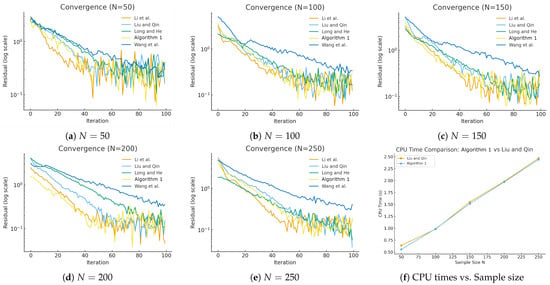
Figure 1. Comaprsion for $N=50,100,150,200,250$ (Algorithm 1,30,31,38,43]).

Table 2 below shows all algorithms converging across sample sizes. Algorithm 1 achieve balanced performance, requiring fewer iterations than Wang et al. [30] and Liu and Qin [31], while maintaining a competitive speed similar to Li et al. [43]. Its strength lies in combining stability with efficiency, offering reliable convergence under varying sample sizes. However, it should be noted that Long and He [38] achieve the fastest. Their algorithm is non-monotone, Lipschitz continuous with one oracle call per iteration, while Algorithm 1 have two oracle calls per iteration (see [38], Remark 1(i), Table 1).

Table 2. Convergence summary for the five algorithms across different sample sizes N.

Algorithm	$\mathit{N}=50$			$\mathit{N}=100$			$\mathit{N}=150$			$\mathit{N}=200$			$\mathit{N}=250$
	Time (s)	Iter	Conv	Time (s)	Iter	Conv	Time (s)	Iter	Conv	Time (s)	Iter	Conv	Time (s)	Iter	Conv
Li et al. [43]	0.002	35	Yes	0.003	30	Yes	0.004	28	Yes	0.005	27	Yes	0.006	25	Yes
Liu and Qin [31]	0.002	40	Yes	0.004	36	Yes	0.004	33	Yes	0.005	31	Yes	0.006	29	Yes
Long and He [38]	0.001	32	Yes	0.002	29	Yes	0.003	27	Yes	0.003	25	Yes	0.004	24	Yes
Algorithm 1	0.002	38	Yes	0.003	34	Yes	0.004	31	Yes	0.004	29	Yes	0.005	28	Yes
Wang et al. [30]	0.001	45	Yes	0.002	41	Yes	0.003	39	Yes	0.004	36	Yes	0.004	34	Yes

Example 2. (Network Bandwidth allocation) We consider a communication network in which individual users, acting selfishly, compete for shared bandwidth resources. The set of all users in a network is indexed by $S:=\{1,2,\dots ,m\}.$ Noting that each user can access multiple routes, one assumes that $\mathsf{\Phi }\left(s\right)$ is the set of routes governed by users $s\in S.$ For $s\in S,$ let $\vartheta \left(s\right)$ denotes the number of elements in $\mathsf{\Phi }\left(s\right)$ and $\Theta :={\sum }_{s\in S}\vartheta \left(s\right).$ Let $x_s^r(r\in \mathsf{\Phi })\left(s\right)$ be the flow rate for users s through which route r goes. The set of all links is denoted by $\mathbb{L}:=\{1,2,\dots ,\kappa .\}.$ The set of routes is denoted by $R:=\{1,2,\dots ,t\}.$ For $d\in \mathbb{L},$ one assumes that ${\mathbb{L}}_s^{\left(t\right)}$ is the set of links through which route $t\in \mathsf{\Phi }\left(s\right)$ goes. Suppose that

$$\begin{array}{c}\hfill {\mathcal{X}}_{s,d}^t=\left\{\begin{array}{c}1,ifd\in {\mathbb{L}}_s^{\left(t\right)};\hfill \\ 0,otherwise.\hfill \end{array}\right.\end{array}$$

When the flow rate is allocated to a user participating in a network, it derives a utility modeled as the value of a concave function. The utility function of each user is parametrized by the uncertainty, which is defined by

$$f_s(x_s,{\xi }_s):=\sum _{r\in \vartheta \left(s\right)}{\xi }_s^{\left(r\right)}In(1+x_s^r),\forall s\in S,$$

where $x_s:={\left(x_s^{\left(r\right)}\right)}_{r\in \mathsf{\Phi }\left(s\right)}$ is the flow rate decision vector of users, ${\xi }_s^r$ is the random weighted parameter route $r\in \mathsf{\Phi }\left(s\right),$ and ${\xi }_s:={\left({\xi }_s^r\right)}_{r\in \mathsf{\Phi }\left(s\right)}.$ The flow rate allocated to each user is regulated with a control mechanism to prevent network congestion in the bandwidth allocation. Such a mechanism ensures that the sum of the transmission rate for users sharing the link $\nu \in \mathbb{L}$ is less than or equal to the limited capacity of the link $t,$ that is,

$${\mathbb{X}}_{\nu }:=\left\{{\left({\left(x_s^{\left(r\right)}\right)}_{r\in \vartheta \left(s\right)}\right)}_{s\in S}\in {\mathbb{R}}_{+}^{\Theta }:\sum _{s\in S}{x}_s^{\left(r\right)}{X}_{s,d}^t\le c_{\nu },\right\},$$

where $c_t>0$ is the capacity of link $t\in \mathbb{L}.$ Set $c:={\left(c_t\right)}_{t\in \mathbb{L}}.$

We now formulate this model as a stochastic optimization problem given by

$$\begin{array}{c}\hfill maximize\sum _{\mathbb{E}}\left[f_s(x_s,{\xi }_s)\right]\\ \hfill subjecttox:={\left({\left(x_s^{\left(r\right)}\right)}_{r\in \mathsf{\Phi }\left(s\right)}\right)}_{s\in S}\in {\cap }_{t\in \mathbb{L}}{\mathbb{X}}_t,\end{array}$$

(46)

Let $\mathcal{M}$ denote the adjacency matrix that describes the correlation between the set of links $\mathbb{L}$ and the set of routes $R:={\cup }_{s\in S}\left(\vartheta \left(s\right)\right).$ We assumes that ${\mathcal{M}}_{t,r}:=1$ if route $r\in R$ goes through link $\nu \in \mathbb{L},$ otherwise $0.$ We observe that problem (46) can be captured by an SVI in a compact form:

Find $x^{\ast }\in \mathbb{X}:={\cap }_{\nu \in \mathbb{L}}{\mathcal{X}}_t,$ such that

$$⟨F\left(x^{\ast }\right),x-x^{\ast }⟩\ge 0,$$

for any $x\in {\cap }_{t\in \mathbb{L}},$ where

$$\begin{array}{ccc}\hfill F\left(x\right):& =& \nabla \left(-\sum _{s\in S}\mathbb{E}\left[f_s(x_s,{\xi }_s)\right]\right)\hfill \\ & =& -{\left({\displaystyle \frac{\mathbb{E}\left[{\xi }_s^r\right]}{1+x_s^{\left(r\right)}}}\right)}_{s\in S},\hfill \end{array}$$

(47)

and

$$\begin{array}{c}\hfill \mathcal{X}:=\{{\left({\left(x_s^{\left(r\right)}\right)}_{r\in \vartheta \left(s\right)}\right)}_{s\in S}\in {\mathbb{R}}_{+}^{\Theta }:\mathcal{M}\left(x\right)\le c\}.\end{array}$$

(48)

Now, we consider the bandwidth allocation problem on a network that consists of 10 nodes, 10 links, and 2 users. It is observed that $S:=\{1,2\},\mathbb{L}:=\{1,2,\dots ,10\},R:\{1,2,\dots ,5\},\mathsf{\Phi }\left(1\right):=\{1,2\}$ and $\mathsf{\Phi }\left(2\right)=\{1,2,3\}.$

In this experiment, the weighted parameters ${\xi }_s^r(s\in S,r\in \vartheta \left(s\right))$ are i.i.d. and drawn randomly from the uniform distribution according to Table 1. Beside, the links have limited capacity $c:=\left(c_{\nu \in \mathbb{L}}\right)$ with the values $c_1,\dots ,c_5$ given Table 2. One can check that the involved operator $F(.)$ in (47) is quasi-monotone and Lipschitz continuous in $\mathbb{X}$ with the constant $\mathbb{L}\left(\xi \right):={max}_{s\in S,r\in \vartheta \left(s\right)}{\xi }_s^r+2\parallel {\mathbb{MM}}^T\parallel .$

Figure 2 below shows a network of 10 nodes, 10 links, and 5 routes connecting two users. Core links carry higher capacities to support aggregate flows, while edge links act as potential bottlenecks. Shared routes between users highlight congestion risks, emphasizing the importance of efficient bandwidth allocation and resource management.

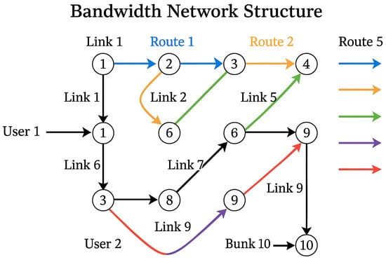
Figure 2. The bandwidth allocation network structure.

Table 3 presents uniform distributions of random parameters for each user’s routes. These ranges capture uncertainty in flow performance, modeling variability in network conditions, and ensuring fairness during bandwidth allocation.

Table 3. Uniform distribution of randomly generated parameters ${\xi }_s^r$ for each user-route pair.

User	Route	Random Parameter ${\mathit{\xi }}_{\mathit{s}}^{\mathit{r}}$	Distribution Range
User 1	$R_1$	${\xi }_1^{\left(1\right)}$	$\mathcal{U}(0.8,1.2)$
	$R_2$	${\xi }_1^{\left(2\right)}$	$\mathcal{U}(0.7,1.3)$
User 2	$R_1$	${\xi }_2^{\left(1\right)}$	$\mathcal{U}(0.9,1.4)$
	$R_2$	${\xi }_2^{\left(2\right)}$	$\mathcal{U}(0.6,1.1)$
	$R_3$	${\xi }_2^{\left(3\right)}$	$\mathcal{U}(0.75,1.25)$

Table 4 below reveals how different links are utilized in optimized flow allocation. Heavily loaded links like 4 and 8 should be carefully monitored or upgraded in real networks, while lightly loaded links like 6 and 7 might indicate insufficient routing or a redundant path. NB:Mbps means megabits per second and Gbps means gigabits per second.

Table 4. Link capacities $c_{\nu }$ (sample values). Units: flow units (replace with Mbps/Gbps as needed).

Link $\mathit{\nu }$	Incident Routes	Example Load	Suggested Capacity ${\mathit{c}}_{\mathit{\nu }}$	Slack (${\mathit{c}}_{\mathit{t}}$-Load)
1	{1}	$0.693$	$1.386$	$0.693$
2	{1,2}	$1.118$	$2.235$	$1.117$
3	{1,2}	$1.118$	$2.235$	$1.117$
4	{2,3}	$1.512$	$3.024$	$1.512$
5	{3}	$1.088$	$2.175$	$1.088$
6	{4}	$0.471$	$0.942$	$0.471$
7	{4}	$0.471$	$0.942$	$0.471$
8	{4,5}	$1.207$	$2.414$	$1.207$
9	{5}	$0.736$	$1.471$	$0.736$
10	{5}	$0.736$	$1.471$	$0.736$

Example 3. (Networked stochastic Nash–Cournot game) In this experiment, we consider a networked Nash–Cournot game adopted in [44] under uncertainty data, in which the cost-minimizing agents compete in quantity levels when facing a price function associated with aggregate output. Suppose that there are Ω firms that compete over a network of Λ nodes in supplying a homogeneous product in a non-cooperative sense. Let $x_{i,j}$ denote the level of sales of firm $i\in \left[\mathsf{\Omega }\right]$ and at a node $j\in \left[\mathsf{\Lambda }\right]$. Assume that the firm is characterized by a random linear cost function $c_i(X_i,{\xi }_i)=(a_i,{\xi }_i){\sum }_{j\in \left[\mathsf{\Lambda }\right]}{X}_{i,j}$ for some parameters $a_i>0\forall i,$ where ${\xi }_i$ is a mean zero random variable. We assume that the price at node j represented by $P_j({\sum }_{i\in \left[\mathsf{\Omega }\right]}{x}_{i,j},{\eta }_j)$ is a stochastic linear function corrupted by noisy $P_j({\sum }_{i\in \left[\mathsf{\Omega }\right]}{X}_{i,j},{\eta }_j)=d_j+{\eta }_j-b_j{\sum }_{i\in \left[\mathsf{\Omega }\right]}{q}_{i,j},$ where $d_j$ indicates the price when then production is zero, $b_j$ is the slope at the inverse demand function while ${\eta }_j$ is a zero-mean random disturbance. Assume that the transport cost is zero. Except for non-negativity constraints in $x_{i,j},$ we suppose that the firms $i^{\prime }s$ production at node j is capacitated by $ca{p}_{i,j}.$ We now transform the firm $i^{\prime }s$ into stochastic optimization problem given below:

$$\begin{array}{c}\hfill min\mathbb{E}\left[f_i(x,\xi ,\eta )\right]=\mathbb{E}\left[c_i(X_i,{\xi }_i)-\sum _{j\in \left[\mathsf{\Lambda }\right]}{P}_j\left(\sum _{i\in \left[\mathsf{\Omega }\right]}{X}_{i,j},{\eta }_j\right)X_{i,j}\right]\\ \hfill s.t.x_i\in {\mathcal{X}}_i=\{x_i\in {\mathbb{R}}^{\mathsf{\Lambda }}:x_i>0,x_{i,j}\le ca{p}_{i,j}\}\end{array}$$

(49)

Under some dominated conditions, when we interchange the others of expectation and derivative, the above stochastic Nash–Cournot game may be transformed into problem (3) with $\mathcal{X}={\prod }_{i=1}^{\mathsf{\Omega }}{\mathcal{X}}_i$ and $F\left(x\right)=(F_1\left(x\right);\dots ;F_{\mathsf{\Omega }}\left(x\right))$ with $F_i\left(x\right)=\mathbb{E}\left[{\partial }_{x_i}{f}_i(x,\xi ,\eta )\right].$ Just like in [44], we consider a network with $\mathsf{\Omega }=20$ firms, $\mathsf{\Lambda }=10$ markets and the capacity $Ca{p}_{i,j}=2$ for each $\in \in \mathsf{\Omega }$ and each $j\in \mathsf{\Lambda }.$ In the experiment, the parameters in the payoffs were set as $d\approx \mathcal{U}(40,50),b_j\approx \mathcal{U}(1,2),a_i\approx (3,5)$ for all $i\in \left[\mathsf{\Omega }\right]$ and $j\in \left[\mathsf{\Lambda }\right],$ where $\mathcal{U}(u^1,u^2)$ denotes the uniform distribution over an interval $(u^1,u^2),$ where $u^1<u^2.$ For the random data in the model, we assume ${\xi }_i\approx \mathcal{U}({\displaystyle \frac{-a_i}{5}},{\displaystyle \frac{a_i}{5}})$ and ${\eta }_j\approx \mathcal{U}(-{\displaystyle \frac{b_j}{5}},{\displaystyle \frac{b_j}{5}}),x_0=x_{-1}={(1,\dots ,1)}^T$ for all the algorithm.

Figure 3 shows performance comparison of algorithms across convergence behavior, computational efficiency, and underlying network structure.

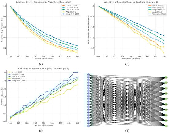
Figure 3. Networked stochastic Nash–Cournot game. (a) Empirical gap-function error, the error decreases across all algorithms, with Algorithm 1 converging fastest, Li et al. [43] closely following, while Liu and Qin [31], Long and He [38], and Wang et al. [30] converge slower. (b) Logarithm of empirical error, the plot shows faster convergence for Algorithm 1, while Wang et al. [30] lags behind, confirming differences in algorithmic efficiency. (c) CPU time, Algorithm 1 requires the least computation, reflecting efficiency, while Wang et al. [30] consumes the most, indicating higher computational overhead. (d) Network structure, twenty firms are interconnected with ten markets, highlighting competitive supply interactions and capacity-constrained distribution across nodes.

Table 5 below highlights uniform link capacities of two across all firm–market connections, while market prices vary stochastically through demand parameters. This structure reflects balanced competition, ensuring equal production opportunities for all firms, while random price variations across markets capture uncertainty and heterogeneity in the Nash–Cournot game environment.

Table 5. Capacity with respect to price, market, and firm.

Market	Price Parameters $({\mathit{d}}_{\mathit{j}},{\mathit{b}}_{\mathit{j}})$	Firms Connected	Capacity per Link
Market 1	$d_1\sim \mathcal{U}(40,50),b_1\sim \mathcal{U}(1,2)$	Firm 1–Firm 20	2
Market 2	$d_2\sim \mathcal{U}(40,50),b_2\sim \mathcal{U}(1,2)$	Firm 1–Firm 20	2
Market 3	$d_3\sim \mathcal{U}(40,50),b_3\sim \mathcal{U}(1,2)$	Firm 1–Firm 20	2
Market 4	$d_4\sim \mathcal{U}(40,50),b_4\sim \mathcal{U}(1,2)$	Firm 1–Firm 20	2
Market 5	$d_5\sim \mathcal{U}(40,50),b_5\sim \mathcal{U}(1,2)$	Firm 1–Firm 20	2
Market 6	$d_6\sim \mathcal{U}(40,50),b_6\sim \mathcal{U}(1,2)$	Firm 1–Firm 20	2
Market 7	$d_7\sim \mathcal{U}(40,50),b_7\sim \mathcal{U}(1,2)$	Firm 1–Firm 20	2
Market 8	$d_8\sim \mathcal{U}(40,50),b_8\sim \mathcal{U}(1,2)$	Firm 1–Firm 20	2
Market 9	$d_9\sim \mathcal{U}(40,50),b_9\sim \mathcal{U}(1,2)$	Firm 1–Firm 20	2
Market 10	$d_{10}\sim \mathcal{U}(40,50),b_{10}\sim \mathcal{U}(1,2)$	Firm 1–Firm 20	2

6. Conclusions

This work introduced an adaptive inertial stochastic projection framework for solving stochastic variational inequalities whose cost function is quasi-monotone, and the developed scheme was applied to stochastic complementary problems, networked stochastic Nash–Cournot game, and bandwidth allocation problem. By combining inertia with adaptive stepsize selection, the method accelerates convergence while preserving robustness under uncertainty. Stochastic projections ensure feasibility with link capacity constraints, preventing congestion and promoting fairness. Numerical experiments demonstrate superior efficiency, scalability, and stability compared to conventional techniques. Beyond bandwidth allocation, the approach offers a versatile tool for stochastic optimization problems in uncertain environments. In a nutshell, the algorithm delivered a resilient and computationally efficient solution, advancing both theory and practice in modern network resource management.

References

- Royset, J.O. Risk-adaptive approaches to stochastic optimization: A survey. SIAM Rev. 2025, 67, 3–70. [Google Scholar] [CrossRef]
- Liang, H.; Zhuang, W. Stochastic modeling and optimization in a microgrid: A survey. Energies 2014, 7, 2027–2050. [Google Scholar] [CrossRef]
- Sclocchi, A.; Wyart, M. On the different regimes of stochastic gradient descent. Proc. Natl. Acad. Sci. USA 2024, 121, e2316301121. [Google Scholar] [CrossRef]
- Dong, D.; Liu, J.; Tang, G. Sample average approximation for stochastic vector variational inequalities. Appl. Anal. 2023, 103, 1649–1668. [Google Scholar] [CrossRef]
- Robbins, H.; Monro, S. A stochastic approximation method. Ann. Math. Stat. 1951, 22, 400–407. [Google Scholar] [CrossRef]
- Farh, H.M.H.; Al-Shamma’a, A.A.; Alaql, F.; Omotoso, H.O.; Alfraidi, W.; Mohamed, M.A. Optimization and uncertainty analysis of hybrid energy systems using Monte Carlo simulation integrated with genetic algorithm. Comput. Electr. Eng. 2024, 120, 109833. [Google Scholar] [CrossRef]
- Stampacchia, G. Formes bilinéaires coercitives sur les ensembles convexes. Comptes Rendus l’Académie Sci. Série A 1964, 258, 4413–4416. [Google Scholar]
- Nagurney, A. Network Economics: A Variational Inequality Approach; Kluwer Academic: Dordrecht, The Netherlands, 1999. [Google Scholar]
- Shehu, Y.; Iyiola, O.S.; Reich, S. A modified inertial subgradient extragradient method for solving variational inequalities. Optim. Eng. 2022, 23, 421–449. [Google Scholar] [CrossRef]
- Liu, L.; Cho, S.Y.; Yao, J.C. Convergence analysis of an inertial Tseng’s extragradient algorithm for solving pseudomonotone variational inequalities and applications. J. Nonlinear Var. Anal. 2021, 2, 47–63. [Google Scholar]
- Nwawuru, F.O.; Echezona, G.N.; Okeke, C.C. Finding a common solution of variational inequality and fixed point problems using subgradient extragradient techniques. Rend. Circ. Mat. Palermo II Ser. 2024, 73, 1255–1275. [Google Scholar] [CrossRef]
- Dilshad, M.; Alamrani, F.M.; Alamer, A.; Alshaban, E.; Alshehri, M.G. Viscosity-type inertial iterative methods for variational inclusion and fixed point problems. AIMS Math. 2024, 9, 18553–18573. [Google Scholar] [CrossRef]
- Facchinei, F.; Pang, J.S. Finite-Dimensional Variational Inequalities and Complementarity Problems; Springer: New York, NY, USA, 2003. [Google Scholar]
- Jiang, H.; Xu, H. Stochastic approximation approaches to stochastic variational inequality problems. IEEE Trans. Autom. Control 2008, 53, 1462–1475. [Google Scholar] [CrossRef]
- Shapiro, A. Monte Carlo sampling methods. In Handbooks in Operations Research and Management Science: Stochastic Programming; Ruszczyński, A., Shapiro, A., Eds.; Elsevier: Amsterdam, The Netherlands, 2003; pp. 353–425. [Google Scholar]
- Wang, M.Z.; Lin, G.H.; Gao, Y.L.; Ali, M.M. Sample average approximation method for a class of stochastic variational inequality problems. J. Syst. Sci. Complex. 2011, 24, 1143–1153. [Google Scholar] [CrossRef]
- He, S.X.; Zhang, P.; Hu, X.; Hu, R. A sample average approximation method based on a D-gap function for stochastic variational inequality problems. J. Ind. Manag. Optim. 2014, 10, 977–987. [Google Scholar] [CrossRef]
- Cherukuri, A. Sample average approximation of conditional value-at-risk based variational inequalities. Optim. Lett. 2024, 18, 471–496. [Google Scholar] [CrossRef]
- Zhou, Z.; Honnappa, H.; Pasupathy, R. Drift optimization of regulated stochastic models using sample average approximation. arXiv 2025, arXiv:2506.06723. [Google Scholar] [CrossRef]
- Yousefian, F.; Nedić, A.; Shanbhag, U.V. Distributed adaptive steplength stochastic approximation schemes for Cartesian stochastic variational inequality problems. arXiv 2013, arXiv:1301.1711. [Google Scholar] [CrossRef]
- Koshal, J.; Nedić, A.; Shanbhag, U.V. Regularized iterative stochastic approximation methods for stochastic variational inequality problems. IEEE Trans. Autom. Control 2013, 58, 594–609. [Google Scholar] [CrossRef]
- Iusem, A.N.; Jofré, A.; Thompson, P. Incremental constraint projection methods for monotone stochastic variational inequalities. Math. Oper. Res. 2019, 44, 236–263. [Google Scholar] [CrossRef]
- Yang, Z.P.; Zhang, J.; Wang, Y.; Lin, G.H. Variance-based subgradient extragradient method for stochastic variational inequality problems. J. Sci. Comput. 2021, 89, 4. [Google Scholar] [CrossRef]
- Korpelevich, G.M. The extragradient method for finding saddle points and other problems. Matekon 1976, 12, 747–756. [Google Scholar]
- Iusem, A.N.; Jofré, A.; Oliveira, R.I.; Thompson, P. Extragradient method with variance reduction for stochastic variational inequalities. SIAM J. Optim. 2017, 27, 686–724. [Google Scholar] [CrossRef]
- Nwawuru, F.O. Approximation of solutions of split monotone variational inclusion problems and fixed point problems. Pan-Am. J. Math. 2023, 2, 1. [Google Scholar] [CrossRef]
- Iusem, A.N.; Jofré, A.; Oliveira, R.I.; Thompson, P. Variance-based extragradient methods with line search for stochastic variational inequalities. SIAM J. Optim. 2019, 29, 175–206. [Google Scholar] [CrossRef]
- Censor, Y.; Gibali, A.; Reich, S. The subgradient extragradient method for solving variational inequalities in Hilbert space. J. Optim. Theory Appl. 2011, 148, 318–335. [Google Scholar] [CrossRef]
- Nwawuru, F.O.; Ezeora, J.N.; ur Rehman, H.; Yao, J.-C. Self-adaptive subgradient extragradient algorithm for solving equilibrium and fixed point problems in Hilbert spaces. Numer. Algorithms 2025. [Google Scholar] [CrossRef]
- Wang, S.; Tao, H.; Lin, R.; Cho, Y.J. A self-adaptive stochastic subgradient extragradient algorithm for the stochastic pseudomonotone variational inequality problem with application. Z. Angew. Math. Phys. 2022, 73, 164. [Google Scholar] [CrossRef]
- Liu, L.; Qin, X. An accelerated stochastic extragradient-like algorithm with new stepsize rules for stochastic variational inequalities. Comput. Math. Appl. 2024, 163, 117–135. [Google Scholar] [CrossRef]
- Polyak, B.T. Some methods of speeding up the convergence of iterative methods. USSR Comput. Math. Math. Phys. 1964, 4, 1–17. [Google Scholar] [CrossRef]
- Nwawuru, F.O.; Ezeora, J.N. Inertial-based extragradient algorithm for approximating a common solution of split-equilibrium problems and fixed-point problems of nonexpansive semigroups. J. Inequalities Appl. 2023, 2023, 22. [Google Scholar] [CrossRef]
- Ezeora, J.N.; Enyi, C.D.; Nwawuru, F.O.; Ogbonna, R.C. An algorithm for split equilibrium and fixed-point problems using inertial extragradient techniques. Comput. Appl. Math. 2023, 42, 103. [Google Scholar] [CrossRef]
- Nwawuru, F.O.; Narian, O.; Dilshad, M.; Ezeora, J.N. Splitting method involving two-step inertial iterations for solving inclusion and fixed point problems with applications. Fixed Point Theory Algorithms Sci. Eng. 2025, 2025, 8. [Google Scholar] [CrossRef]
- Enyi, C.D.; Ezeora, J.N.; Ugwunnadi, G.C.; Nwawuru, F.O.; Mukiawa, S.E. Generalized split feasibility problem: Solution by iteration. Carpathian J. Math. 2024, 40, 655–679. [Google Scholar] [CrossRef]
- Nesterov, Y.E. A method for solving a convex programming problem with convergence rate O(1/k2). Dokl. Akad. Nauk SSSR 1983, 269, 543–547. [Google Scholar]
- Long, X.J.; He, Y.H. A fast stochastic approximation-based subgradient extragradient algorithm with variance reduction for solving stochastic variational inequality problems. J. Comput. Appl. Math. 2023, 420, 114786. [Google Scholar] [CrossRef]
- Zhang, X.; Du, X.; Yang, Z.; Lin, G. An infeasible stochastic approximation and projection algorithm for stochastic variational inequalities. J. Optim. Theory Appl. 2019, 183, 1053–1076. [Google Scholar] [CrossRef]
- Fang, C.; Chen, S. Some extragradient algorithms for variational inequalities. In Advances in Variational and Hemivariational Inequalities; Han, W., Migórski, S., Sofonea, M., Eds.; Advances in Mechanics and Mathematics; Springer: Cham, Switzerland, 2015; Volume 33, pp. 145–171. [Google Scholar]
- Ezeora, J.N.; Nwawuru, F.O. An inertial-based hybrid and shrinking projection methods for solving split common fixed point problems in real reflexive spaces. Int. J. Nonlinear Anal. Appl. 2023, 14, 2541–2556. [Google Scholar]
- Robbins, H.; Siegmund, D. A convergence theorem for nonnegative almost supermartingales and some applications. In Optimizing Methods in Statistics; Rustagi, J.S., Ed.; Academic Press: New York, NY, USA, 1971; pp. 233–257. [Google Scholar]
- Li, T.; Cai, X.; Song, Y.; Ma, Y. Improved variance reduction extragradient method with line search for stochastic variational inequalities. J. Glob. Optim. 2023, 87, 423–446. [Google Scholar] [CrossRef]
- Yang, Z.P.; Lin, G.H. Variance-based single-call proximal extragradient algorithms for stochastic mixed variational inequalities. J. Optim. Theory Appl. 2021, 190, 393–427. [Google Scholar] [CrossRef]
Disclaimer/Publisher’s Note: The statements, opinions and data contained in all publications are solely those of the individual author(s) and contributor(s) and not of MDPI and/or the editor(s). MDPI and/or the editor(s) disclaim responsibility for any injury to people or property resulting from any ideas, methods, instructions or products referred to in the content. |
© 2025 by the authors. Licensee MDPI, Basel, Switzerland. This article is an open access article distributed under the terms and conditions of the Creative Commons Attribution (CC BY) license (https://creativecommons.org/licenses/by/4.0/).