Abstract
This paper addresses first- and second-kind Volterra integral equations (VIEs) with discontinuous kernels. A hybrid method combining the Homotopy Analysis Method (HAM) and Physics-Informed Neural Networks (PINNs) is developed. The convergence of the HAM is analyzed. Benchmark examples confirm that the proposed HAM-PINNs approach achieves high accuracy and robustness, demonstrating its effectiveness for complex kernel structures.
Keywords:
Volterra integral equation; discontinuous kernel; homotopy analysis method; physics-informed neural networks MSC:
45D05; 65R20; 68T07
1. Introduction
VIEs of the first and second kinds are fundamental tools for modeling processes with memory and hereditary effects. In particular, first-kind equations, where the unknown appears only under the integral, often arise in inverse problems and are generally ill-posed. Second-kind equations, in which the unknown function appears both inside and outside the integral, are typically well-posed and suitable for forward modeling. Two important areas where VIEs play a significant role are energy systems and biology. In energy systems, they provide effective models for load leveling in batteries, where the future state depends on both current demand and historical usage. In biology, they are widely used to describe population dynamics, incorporating the influence of past generations on current growth. A wide range of analytical and numerical approaches have been developed for solving VIEs. For instance, spectral and superconvergent techniques have been proposed for both linear and nonlinear systems [1,2], while quadrature-based formulations such as barycentric rational Hermite methods have been introduced for improved numerical integration [3]. Discretization and extrapolation strategies for multidimensional cases have also been investigated [4]. Earlier works employed wavelet-based approaches [5], variational iteration [6], and sinc-collocation schemes [7], alongside semi-analytical methods like the homotopy analysis method [8] and Tau collocation [9]. To address discontinuities in kernels, the Adomian decomposition method has been applied [10], whereas reproducing kernel methods [11] and radial basis function approximations [12] offer alternative function-based formulations. More recently, artificial neural networks have been explored as flexible approximators for VIEs [13]. Together, these contributions highlight the richness of methodologies available for tackling both theoretical and application-oriented integral equation problems.
In this paper, we focus on solving first- and second-kind VIEs with discontinuous kernels because of their applications in load leveling problems in batteries. The general form of this problem can be presented as
where indicates whether the equation is of the first kind () or second kind (). The function F can be linear or nonlinear and is a known function. The kernel is assumed to be discontinuous along a finite number of smooth curves , for , which partition the integration domain as follows:
In light of these discontinuities, Equation (1) can be rewritten in a piecewise integrated form as follows:
It should be noted that the non-negativity of the solution in the load leveling problem for energy systems has already been assumed. The first kind of this problem is among inverse problems, which need some special methods for solving. Falaleev et al. and Sidorov et al. discussed the generalized solution of this problem in [14]. In [15], the existence of a solution for the first-kind problem has been discussed theoretically. In [16], the successive approximation method has been applied for finding the numerical solution for the non-regular case. The paper in [17] presents the parametric families of solutions for the first-kind problem with piecewise smooth kernel. And finally, more theory and basis of these problems can be found in the book in [18]. Among the methods for solving these problems in both the linear and nonlinear cases as well as for the first and second kinds with a prediction on load leveling in batteries, we can mention [19,20]. Also, other methods for solving IEs can be found in [21,22,23].
The HAM is a powerful semi-analytical technique for solving a wide range of linear and nonlinear problems in mathematics, physics, and engineering, which has been presented for the first time by Liao [24]. The main distinctions between the HAM and other methods such as collocation based methods, ADM, HPM, and others lie in the presence of the convergence control parameter ℏ and two additional auxiliary components: the auxiliary function and the auxiliary linear operator L. The function introduces flexibility by allowing the construction of solutions using different functional forms, such as exponential or trigonometric functions, among others, depending on the nature of the problem. A notable feature of the HAM is the parameter ℏ, which provides direct control over the convergence of the approximate series solution. By plotting the so-called ℏ-curves, one can determine the admissible convergence regions; as demonstrated by Liao in [24], the valid region corresponds to the portion of the ℏ-curve that remains parallel to the horizontal axis. Furthermore, the choice of the linear operator L improves the adaptability of the HAM. In this study, we consider the simplest case ; however, more sophisticated operators, such as the Laplace operator or other integral transforms, can be employed to obtain more accurate and efficient solutions. These flexibilities allow the HAM to handle nonlinear equations, integral equations, differential equations, integro-differential equations, and even systems with discontinuities or singularities [25]. It has been successfully applied in fluid dynamics, heat and mass transfer, nonlinear oscillations, wave propagation, biological systems, and financial modeling [26]. Its capability to provide accurate analytical approximations and to control the convergence region makes the HAM particularly useful in problems where purely numerical or perturbation approaches may fail or offer limited insight [27,28]. PINNs are one of the most popular research areas at this time, which allows us to integrate neural networks with the physical laws of the governing system, often expressed by differential equations or IEs [29]. This methodology creates a neural networks loss function from physical constraints. Later, we can minimize it, which makes the solution not only accurate but also physically consistent. Many researchers are working on improving numerical methods for different types of IEs, but still numerical methods are facing challenges with complex kernels, high dimensionality, and discontinuous kernels [30,31,32]. Neural networks allow us to solve these problems efficiently thanks to their universal approximation capability and by incorporating integral operators in the learning process. Numerous research studies demonstrate promising results in diverse fields, ranging from computational engineering and physics to finance and biology [29].
This paper is organized as follows: Section 2 provides the necessary preliminaries, where we recall fundamental concepts and notations and introduce the main idea of the HAM as the analytical foundation of our study. Section 3 is devoted to the main theoretical contributions, where we implement the HAM for solving first- and second-kind VIEs with discontinuous kernels and establish a rigorous convergence theorem to guarantee the validity of the proposed series solution. In Section 4, we present the framework of PINNs, define the augmented solution representation, and construct the residual and full loss functions that incorporate both data-driven learning and the governing equations. This section highlights the novelty of combining the HAM with PINNs to enhance accuracy and robustness. Section 5 contains several numerical examples, where the proposed hybrid HAM-PINN approach is applied to handle VIEs with discontinuities, and the results are compared with existing methods to demonstrate the efficiency, accuracy, and stability of the method. Finally, Section 6 concludes the paper with a summary of the main findings, discussion of the theoretical and practical implications, and suggestions for future research directions. The novelty of this work lies in the integration of an analytical series-based method (HAM) with a modern machine learning framework (PINNs) to develop a hybrid approach capable of solving discontinuous-kernel VIEs more effectively, while also providing theoretical convergence guarantees and practical numerical evidence of superiority over existing methods.
2. Preliminaries
Consider the nonlinear equation
where N is a nonlinear operator and is the unknown function to be determined. Based on the classical HAM, the corresponding zero-order deformation equation is formulated as
where ℏ is the convergence-control parameter, L is an auxiliary linear operator, is an initial guess for , is an auxiliary non-zero function, and is an unknown function that depends on the embedding parameter v.
Since ℏ and are non-zero, Equation (3) satisfies the boundary conditions
indicating that as v continuously changes from 0 to 1, deforms from the initial approximation to the exact solution . This continuous transformation is referred to as the homotopy deformation.
By applying Taylor series expansion around , the function can be expressed as
where each component is given by
If the auxiliary elements L, ℏ, , and are chosen appropriately, the series (5) converges at , resulting in the solution
To systematically compute each term , we define the vector
and derive the m-th order deformation equation by differentiating (3) m-times with respect to v, dividing by , and then setting . This yields
where the nonlinear operator is defined as
and is given by
Using the computed terms , the l-th order approximation of the exact solution is
and the exact solution is obtained as the limit
Therefore, the accuracy and convergence of the solution heavily depend on the appropriate choice of auxiliary elements L, ℏ, , and the initial guess .
3. Main Idea
First, we focus on solving the IE (2) when . It means we have a first-kind IE
and if for the nonlinear term, we have , then we get a linear problem like
We can define the operator N as follows:
The n-th order deformation equation of the HAM can be expressed as
where
Substituting Equation (12) into Equation (11), we get
We know that, having freedom to choose the special parameters, operators, and functions of the HAM like , and is one of the advantages of the HAM in comparison to the other semi-analytical methods. By taking in Equation (13) the following successive formula can be obtained:
Applying the successive Formula (14) leads to the M-th order approximate solution of IE (10) using
Then, applying the inverse substitution we find the approximate solution of the nonlinear problem (9).
For the second-kind problem, we have in Equation (2) and we get
and by the same transformation, we can change the problem to the linear form as
Repeating the same process as for the first-kind problem, we have the following successive relations:
and the approximate solution can be found using Equation (15).
It is important to note that the presence of discontinuities in the kernel does not introduce instability in our solution process. This is because the integral equation is explicitly partitioned into subintervals at the discontinuity locations, as shown in Equation (1). Each subinterval is handled separately, which avoids the need for additional “gluing” conditions or smoothness assumptions at the discontinuity points. Consequently, the homotopy analysis framework applies uniformly across all subdomains, and the convergence behavior remains stable near the discontinuities. Our numerical results further confirm that the method produces bounded errors in the vicinity of discontinuity points, demonstrating that they do not disrupt the solution process.
The following flowchart (Figure 1) shows the HAM procedure for solving IEs.
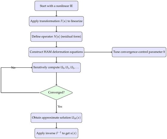
Figure 1.
Flowchart of the HAM procedure for solving nonlinear integral equations.
Theorem 1.
Proof.
The series solution (16) can be written as follows:
where . Using Equation (6), we have
and for the obtained equation, we get
Applying Equation (21) and using the definition of the linear operator L, we have
Thus,
In the obtained formula . So,
Now, we can write
which shows that the series solution (19) must be the exact solution as that of problem (2).
In the HAM, ℏ is known as the deformation parameter. Choosing an optimal ℏ is very important to control error. We can choose an optimal ℏ from the ℏ curve where it is flat in our numerical illustration. □
4. Physics-Informed Neural Networks Integration
The proposed method integrates the HAM with PINNs. The combined algorithm is more powerful to capture the accurate solution pattern. The HAM captures the fundamental behavior of the solution, while neural networks make it more refined to the exact solution by minimizing the loss function of the governing integral equation.
The neural network of HAM-PINN is a fully connected feed-forward network (Figure 2). The network consists of a single input layer, three hidden layers, and one output layer. In the input layer, there is only a single neuron, which takes the independent variable t from . In the three hidden layers, there are 40 neurons, which are passed through the hyperbolic tangent activation function, which normalizes the output to the range . The final layer is the output layer with the single neuron, which approximates the overall solution. To optimize the parameters, we use the Adam optimizer with an initial learning rate of , and the model is trained for a total of 3000 epochs.
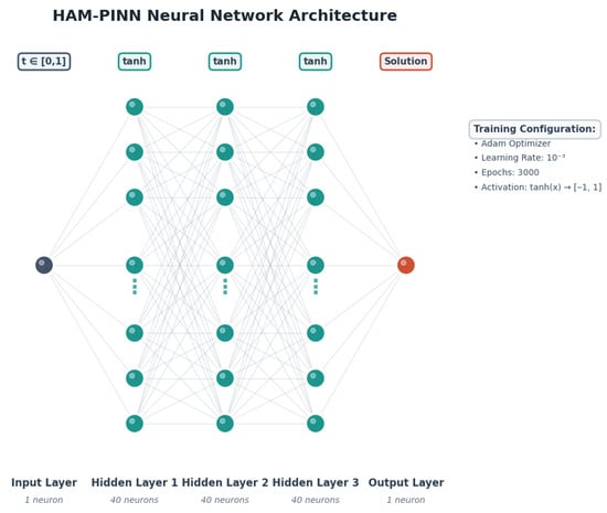
Figure 2.
Schematic flow.
4.1. Augmented Solution
The total approximate solution is the solution from the HAM series with optimized order and optimized h. After all, the additional neural network to the approximate solution is the extra correction term, which allows us to obtain a more refined result.
where represents the sum of the first N terms of the HAM series for a specific or most optimized value of h, which is pre-computed and fixed during the neural networks training. denotes the output of a feed-forward neural networks where the goal is to achieve the most optimized , which minimizes the loss function, designed to approximate the remaining part of the solution.
4.2. PINN Residual Loss
The main idea of constructing any PINN algorithm lies in designing a physics-informed loss function of the corresponding governing equation of the system. For a VIE of the form (2), the residual loss function is the square of the difference between the left and right sides of the set of points for the integral equation.
where
- is the number of points sampled uniformly or randomly across the domain.
- is the augmented solution evaluated at .
- is the forcing term evaluated at .
- is a constant coefficient from the integral equation.
- represents the numerical approximation of the j-th segment of the integral term at . The integral is often split into multiple segments, especially for discontinuous kernels, as seen in the provided Python 3.12.11 code where the kernel changes over different sub-intervals.
Here, the numerical integration for each segment is performed using a quadrature rule over a grid of integration points :
where is the kernel function specific to the j-th integral segment, evaluated at and integration point with the current estimate of the total solution . is the corresponding quadrature weights, and denotes the set of integration points that fall within the bounds of the j-th integral segment for a given .
4.3. Full Loss Function
The primary focus in PINNs is to minimize the physics-informed residual. PINN frameworks often include regularization terms to remove overfitness and improve training stability and generalization.
where in this context refers to the sum of the weighted squared terms of the parameter . is a hyperparameter that controls the weighting of the regularization term relative to the physics loss. The training process focuses on optimizing to minimize this .
5. Numerical Illustration
In this section, we present several numerical examples involving linear and nonlinear VIEs of both the first and second kinds, characterized by discontinuous kernels. The proposed HAM-PINN method is employed to solve these problems. Our training strategy includes two hidden layers with the 40 neurons, and we used the following relation
as the activation function [33]. We take up to 200 equally independent points x.
Also, in order to compare the accuracy of the method, we focus on three metrics [34], including MSE (Mean Squared Error), MAE (Mean Absolute Error), and R-squared, as follows:
where is to show the obtained numerical solution, is the obtained solution value by PINN, is the average value of all the solution values obtained using the numerical method, and K is the number of time data points. The results are summarized through tables comparing the approximate solutions with the exact ones at various values of t, including the corresponding errors. In addition, graphical illustrations such as the comparison of exact and approximate solutions, loss curves across training epochs, error graphs, and the ℏ-curves are provided for deeper insight.
Example 1.


Consider the following linear Volterra integral equation of the first kind:
where the exact solution is . The HAM-PINN method is applied to solve this equation, using and training the neural networks for 3000 epochs.
Table 1 presents the error metrics for the HAM-PINN solution in Example 1, including the MAE, MSE, and cumulative values. The MAE remains very small across all time points, reaching a maximum of approximately at , indicating that the predicted solution closely aligns with the exact solution. The MSE values are consistently negligible, confirming the stability of the approximation. The cumulative values are all near 1, reflecting strong agreement between the HAM-PINN predictions and the reference solution, except at the initial point where is undefined. Overall, the results indicate that HAM-PINN provides accurate and reliable approximations for this example without significant variation in the error measures across the interval.

Table 1.
Comparison between different errors for HAM-PINN in Example 1.
Table 2 compares the exact solution with the approximate solutions obtained using HAM-PINN and HAM for Example 1, along with their corresponding absolute errors. Overall, HAM-PINN produces results that closely align with the exact solution at all time points, with absolute errors generally on the order of or smaller. In comparison, HAM also provides reasonable approximations, but the errors are slightly higher at intermediate points, such as at and , where HAM-PINN shows improved accuracy. At , HAM achieves a marginally smaller error than HAM-PINN; however, across the majority of the interval, HAM-PINN demonstrates more consistent performance. These results indicate that the hybrid HAM-PINN approach maintains a stable and reliable approximation throughout the domain while effectively handling variations in the solution.

Table 2.
Comparison between the exact and approximate solutions and absolute errors in Example 1.
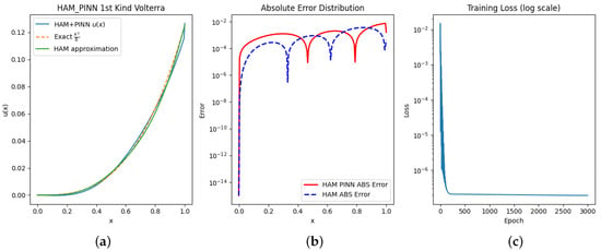
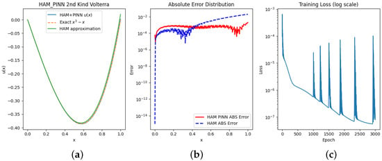
Figure 3a shows the comparative graphs between the approximate and exact solutions. Figure 3b contains the graphs of the absolute errors for HAM and PINN, which shows that PINN has better and accurate results against normal HAM. Figure 3c illustrates the evolution of the loss function during training, highlighting how the networks parameters θ are optimized to minimize the error and enhance model performance.

Figure 3.
(a) Exact and approximate solutions. (b) Absolute error functions. (c) Loss vs. epoch.
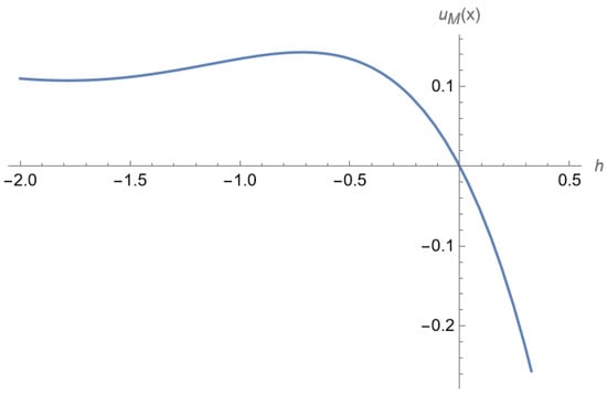
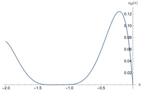
Figure 4 illustrates the convergence region of the auxiliary parameter ℏ, which plays a crucial role in ensuring the validity of the HAM. By plotting the so-called ℏ-curves, we are able to identify the intervals where the approximate solution converges to the exact one. For this particular example, the convergence region is observed within the interval . Inside this range, the series solution generated by the HAM remains stable and reliable, whereas values of ℏ outside this interval lead to divergence or loss of accuracy. This clearly demonstrates the importance of the convergence-control parameter in the HAM, since it not only guarantees convergence but also provides flexibility in adjusting the solution process without altering the original problem formulation.

Figure 4.
ℏ-curve for Example 1 for .
Example 2.


Consider the following Volterra integral equation of the first kind:
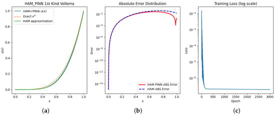
where the exact solution is given by . This equation is characterized by a linear structure and a discontinuous kernel. To solve this problem, we applied a hybrid approach combining the PINN method with the HAM, using and training the neural networks up to 3000 epochs.
Table 3 presents the error analysis of the HAM-PINN method for Example 2. At , all error measures are zero, as expected from the initial condition. For , the method shows a relatively small mean absolute error (MAE = 0.002350), though the value (0.304838) indicates limited agreement with the exact solution at this early stage. As t increases to 0.50 and 0.75, the errors grow moderately (MAE = 0.016805 and 0.022351), but the values improve significantly, suggesting that the approximation follows the overall trend of the exact solution more closely. Finally, at , the method achieves a very low error (MAE = 0.001786) with an of 0.998903, showing strong agreement at the final point.

Table 3.
Comparison between different errors for HAM-PINN in Example 2.
Table 4 compares the exact solution with the HAM-PINN and HAM approximations for Example 2, together with their absolute errors. At , all methods start from the exact value, giving zero error, as expected. For and , both HAM-PINN and HAM provide close approximations, though HAM-PINN shows slightly smaller errors (0.002350 and 0.016805) compared to the HAM (0.002504 and 0.020320). At , the HAM-PINN error is 0.022351, which remains lower than the HAM’s error of 0.035844, indicating a closer alignment with the exact solution in this interval. Finally, at , HAM-PINN achieves a very small error of 0.001786, while the HAM has a larger deviation of 0.012523.

Table 4.
Comparison between the exact and approximate solutions and absolute errors in Example 2.
Figure 5 illustrates different aspects of the results. In panel (a), the solution obtained by the HAM-PINN method shows a close agreement with the exact solution. Panel (b) presents a comparison of the errors from the HAM and HAM-PINN, highlighting their relative accuracy. Panel (c) depicts the convergence trend of the loss function during training, reflecting how the optimization of the neural network parameters θ contributes to improving the solution accuracy.

Figure 5.
(a) Exact and approximate solutions. (b) Absolute error functions. (c) Loss vs. epoch.
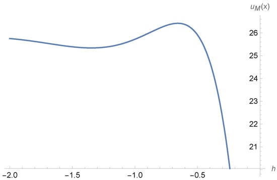
Figure 6 presents the admissible interval of the convergence-control parameter ℏ for this example. The results indicate that the convergence region is obtained within the range for . This interval corresponds to the nearly horizontal portion of the h-curve, which is known to characterize the region where the HAM series solution remains valid and reliable. Identifying such a range is essential, since values of ℏ outside this interval may lead to divergence or reduced accuracy of the approximation.

Figure 6.
Convergence region for ℏ in Example 3.
Example 3.


Consider the following nonlinear VIE
with the exact solution where the source term is
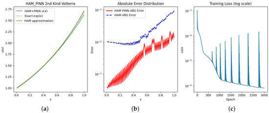
where the exact solution is . Here, we show our result after combining the neural networks training up to 3000 epochs and the HAM for and .
Table 5 presents the error metrics for HAM-PINN in Example 3. At , the MSE is zero. For and , the mean absolute error remains small (0.001459 and 0.002712, respectively), with corresponding MSE values on the order of to . At later points, and , the errors increase slightly, reaching a maximum MAE of 0.013723. Despite this increase, the values remain close to unity (above 0.9998), suggesting that the HAM-PINN solution maintains a strong agreement with the exact solution throughout the interval. The results indicate stable performance of the method, with errors growing moderately as t increases.

Table 5.
Comparison between different errors for HAM-PINN in Example 3.
Table 6 compares the exact solution with the approximations obtained by HAM-PINN and pure HAM in Example 3, together with their absolute errors. At , both methods reproduce the initial condition, but HAM-PINN achieves a smaller error (0.000387) compared to the HAM (0.010050). As t increases, HAM-PINN consistently provides lower errors than HAM. For instance, at and , the absolute errors of HAM-PINN are 0.001459 and 0.002712, respectively, while the HAM errors are noticeably larger (0.008264 and 0.011896). At later points ( and ), the difference becomes more pronounced: HAM-PINN maintains errors below 0.014, whereas the HAM errors increase to 0.035116 and 0.094190. The results indicate that HAM-PINN achieves closer agreement with the exact solution across the whole interval, with a clear improvement in accuracy compared to the HAM, especially at larger values of t.

Table 6.
Comparison between the exact and approximate solutions and absolute errors in Example 3.
Figure 7a shows that the HAM-PINN approach closely aligned with the exact solution, Figure 7b gives a comparison between the errors, and Figure 7c demonstrates how the loss function is optimized per epoch to obtain the promising result by determining θ, which is the parameter of the neural networks.

Figure 7.
(a) Exact and approximate solutions. (b) Absolute error functions. (c) Loss vs. epoch.
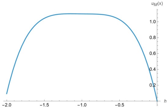
Figure 8 shows the ℏ-curve, illustrating the range of auxiliary parameter ℏ for which the HAM solution converges. For this particular example, convergence is achieved when ℏ lies within the interval . Within this range, the curve exhibits a nearly flat portion that runs parallel to the x-axis, which defines the stable convergence region. This parallel segment indicates that small variations in ℏ do not significantly affect the accuracy of the solution, providing flexibility in selecting the parameter. Outside this interval, the curve deviates sharply, suggesting that the solution may diverge or lose accuracy. Therefore, choosing ℏ from the parallel region ensures both convergence and numerical stability of the HAM approximation.

Figure 8.
ℏ Curve of Example 3 for .
Example 4.


Consider the integral equation:
with
where the exact solution is . This is a linear Volterra IE of the second kind with a discontinuous kernel.
Table 7 presents the error metrics for the HAM-PINN solution in Example 4, including MAE, MSE, and cumulative values. The MAE remains consistently small across all time points, with the highest value being at , indicating that the predicted solution closely follows the exact solution. The MSE values are negligible throughout, reflecting the stability and consistency of the method. The cumulative values are all very close to 1, confirming strong agreement between the HAM-PINN predictions and the reference solution, except at the initial point where is undefined. The results demonstrate that HAM-PINN provides accurate and reliable approximations with stable performance over the entire interval.

Table 7.
Comparison between different errors for HAM-PINN in Example 4.
Table 8 compares the exact solution with the approximate solutions obtained using HAM-PINN and HAM, along with their absolute errors. The HAM-PINN method maintains a close alignment with the exact solution across all time points, with absolute errors ranging from at to at . In comparison, the HAM shows slightly larger deviations, particularly at and , where the absolute error reaches and , respectively. These results indicate that HAM-PINN provides more consistent and accurate approximations, especially in regions affected by rapid changes or near the endpoints, while HAM performs adequately in smoother regions but exhibits larger errors in critical points.

Table 8.
Comparison between the exact and approximate solutions and absolute errors in Example 4.
Figure 9 illustrates different aspects of the HAM-PINN performance. Figure 9a shows that the HAM-PINN solution is closely aligned with the exact solution across the domain. Figure 9b presents a comparison of the absolute errors obtained from HAM-PINNs and pure HAM, highlighting the improved accuracy of the hybrid approach. Finally, Figure 9c displays the evolution of the loss function during training, demonstrating how the neural network parameters θ are progressively optimized to enhance solution accuracy.

Figure 9.
(a) Exact and approximate solutions. (b) Absolute error functions. (c) Loss vs. epoch.
Figure 10 illustrates the admissible range of values for the auxiliary parameter ℏ that ensures a convergent solution. For this problem, convergence is obtained when . Within this interval, the ℏ-curve exhibits a nearly flat portion that runs parallel to the x-axis, indicating a stable convergence region. This parallel behavior suggests that the solution remains insensitive to small variations in ℏ, providing flexibility in its selection without compromising accuracy. Outside this range, however, the curve deviates, leading to divergence and loss of reliability in the approximation. Hence, choosing ℏ from the parallel region ensures both convergence and numerical stability of the solution.

Figure 10.
ℏ curve Example 4 for .
6. Conclusions
In this study, we investigated the numerical solution of first- and second-kind VIEs with discontinuous kernels, which are fundamental in modeling systems with memory effects, such as load leveling in battery energy systems. The discontinuities in the kernels in the load leveling problem introduce significant challenges, requiring robust numerical strategies. To address this, we proposed a hybrid framework that combines the HAM, with its analytical flexibility and adjustable convergence control, and PINNs, which leverage data-driven learning guided by physical laws.
The comparative analysis between the HAM and HAM-PINNs demonstrates that the hybrid method achieves improvements in accuracy. For example, the absolute errors in HAM-PINNs were consistently lower than those of the HAM alone. However, these improvements come at the cost of additional computational effort due to the training phase of PINNs, which requires optimization over neural network parameters. Despite this, the enhanced accuracy and stability make HAM-PINNs a promising trade-off between precision and computational cost.
When compared with existing methods in the literature, the HAM-PINN approach demonstrates strong competitiveness, yielding results that are consistently closer to the exact solutions across various test problems. One of the main advantages of the HAM-based family of methods is the presence of auxiliary functions, auxiliary parameters, and the freedom in selecting a linear operator. These features provide a high degree of flexibility and control over the convergence of the series solution, which is not available in most traditional methods. In particular, the ℏ-curve offers a practical mechanism for identifying convergence regions and ensuring solution stability, allowing the method to be systematically tuned for improved accuracy.
Several limitations of the proposed method should also be noted. The scalability of HAM-PINNs to high-dimensional domains remains challenging due to increased computational demand in training PINNs. Additionally, while the current study focused primarily on linear examples, future work should address nonlinear integral equations and coupled systems to further validate the robustness of the framework.
Looking ahead, future research directions include (i) extending the approach to stochastic kernels and uncertainty quantification, and (ii) developing adaptive real-time learning strategies for online control and energy management. These extensions would enhance the practicality and versatility of HAM-PINNs in solving real-world problems where memory effects and discontinuities play a dominant role.
Author Contributions
Methodology, S.N., M.A.M. and S.M.; Software, S.N. and M.A.M.; Validation, S.N., M.A.M. and S.M.; Formal analysis, S.N. and S.M.; Investigation, S.M.; Writing—original draft, S.N. and M.A.M.; Writing—review & editing, S.N., M.A.M. and S.M. All authors have read and agreed to the published version of the manuscript.
Funding
The work of S. Noeiaghdam was funded by the High-Level Talent Research Start-up Project Funding of Henan Academy of Sciences (Project No. 241819246).
Data Availability Statement
Data are contained within the article.
Conflicts of Interest
The authors declare no conflicts of interest.
References
- Kumar, R.; Kant, K.; Kumar, B.V.R. Superconvergent spectral methods for system of modified Volterra Integral Equations. Math. Comput. Simul. 2026, 239, 115–134. [Google Scholar] [CrossRef]
- Chakraborty, S.; Agrawal, S.K.; Nelakanti, G. Spectral approximated superconvergent methods for system of nonlinear Volterra Hammerstein integral equations. Chaos Solitons Fractals 2025, 192, 116008. [Google Scholar] [CrossRef]
- Abdi, A.; Hormann, K.; Hosseini, S.A. Linear barycentric rational Hermite quadrature and its application to Volterra integral equations. J. Comput. Appl. Math. 2026, 474, 117009. [Google Scholar] [CrossRef]
- Bazm, S.; Lima, P.; Nemati, S. Discretization methods and their extrapolations for two-dimensional nonlinear Volterra-Urysohn integral equations. Appl. Numer. Math. 2025, 208, 323–337. [Google Scholar] [CrossRef]
- Bahmanpour, M.; Araghi, M.A.F. Numerical solution of Fredholm and Volterra integral equations of the first kind using wavelets bases. J. Math. Comput. Sci. 2012, 5, 337–345. [Google Scholar] [CrossRef]
- Araghi, M.A.F.; Behzadi, S.S. Solving nonlinear Volterra–Fredholm integro-differential equations using He’s variational iteration method. Int. J. Comput. Math. 2011, 88, 829–838. [Google Scholar] [CrossRef]
- Fahim, A.; Araghi, M.A.F.; Rashidinia, J.; Jalalvand, M. Numerical solution of Volterra partial integro-differential equations based on sinc-collocation method. Adv. Differ. Equ. 2017, 2017, 362. [Google Scholar] [CrossRef]
- Behzadi, S.S.; Abbasbandy, S.; Allahviranloo, T.; Yildirim, A. Application of homotopy analysis method for solving a class of nonlinear Volterra-Fredholm integro-differential equations. J. Appl. Anal. Comput. 2012, 2, 127–136. [Google Scholar]
- Gouyandeh, Z.; Allahviranloo, T.; Armand, A. Numerical solution of nonlinear Volterra–Fredholm–Hammerstein integral equations via Tau-collocation method with convergence analysis. J. Comput. Appl. Math. 2016, 308, 435–446. [Google Scholar] [CrossRef]
- Amirkhizi, S.A.; Mahmoudi, Y.; Shamloo, A.S. Solution of Volterra integral equations of the first kind with discontinuous kernels by using the Adomian decomposition method. Comput. Methods Differ. Equ. 2024, 12, 189–195. [Google Scholar]
- Amoozad, T.; Allahviranloo, T.; Abbasbandy, S.; Malkhalifeh, M.R. Application of the reproducing kernel method for solving linear Volterra integral equations with variable coefficients. Phys. Scr. 2024, 99, 025246. [Google Scholar] [CrossRef]
- Firouzdor, R.; Asari, S.S.; Amirfakhrian, M. Application of radial basis function to approximate functional integral equations. J. Interpolat. Approx. Sci. Comput. 2016, 2, 77–86. [Google Scholar] [CrossRef]
- Jafarian, A.; Measoomy, S.; Abbasbandy, S. Artificial neural networks based modeling for solving Volterra integral equations system. Appl. Soft Comput. 2015, 27, 391–398. [Google Scholar] [CrossRef]
- Sidorov, N.A.; Falaleev, M.V.; Sidorov, D.N. Generalized solutions of Volterra integral equations of the first kind. Bull. Malays. Math. Sci. Soc. 2006, 28, 101–109. [Google Scholar]
- Sidorov, N.A.; Sidorov, D.N. Existence and construction of generalized solutions of nonlinear Volterra integral equations of the first kind. Differ. Equ. 2006, 42, 1312–1316. [Google Scholar] [CrossRef]
- Sidorov, N.A.; Sidorov, D.N.; Krasnik, A.V. Solution of Volterra operator-integral equations in the nonregular case by the successive approximation method. Differ. Equ. 2010, 46, 882–891. [Google Scholar] [CrossRef]
- Sidorov, D.N. On parametric families of solutions of Volterra integral equations of the first kind with piecewise smooth kernel. Differ. Equ. 2013, 49, 210–216. [Google Scholar] [CrossRef]
- Sidorov, D. Integral Dynamical Models: Singularities. Signals & Control, T. 87; World Scientific Series on Nonlinear Science Series A; World Scientific Publications Pte Ltd.: Singapore, 2015. [Google Scholar]
- Noeiaghdam, S.; Sidorov, D.; Dreglea, A. A novel numerical optimality technique to find the optimal results of Volterra integral equation of the second kind with discontinuous kernel. Appl. Numer. Math. 2023, 186, 202–212. [Google Scholar] [CrossRef]
- Noeiaghdam, S.; Sidorov, D.; Muftahov, I.; Zhukov, A.V. Control of Accuracy on Taylor-Collocation Method for Load Leveling Problem. Bull. Irkutsk. State Univ. Ser. Math. 2019, 30, 59–72. [Google Scholar] [CrossRef]
- Noeiaghdam, S.; Araghi, M.A.F. Homotopy regularization method to solve the singular Volterra integral equations of the first kind. Jordan J. Math. Stat. 2018, 11, 1–12. [Google Scholar]
- Noeiaghdam, S.; Araghi, M.A.F. Valid implementation of the Sinc-collocation method to solve the linear integral equations by CADNA library. J. Math. Model. 2019, 7, 63–84. [Google Scholar]
- Mikaeilvand, N.; Noeiaghdam, S. Mean value theorem for integrals and its application on numerically solving of Fredholm integral equation of second kind with Toeplitz plus Hankel Kernel. Int. J. Ind. Math. 2014, 6, 351–360. [Google Scholar]
- Liao, S.J. The Proposed Homotopy Analysis Techniques for the Solution of Nonlinear Problems. Ph.D. Thesis, Shanghai Jiao Tong University, Shanghai, China, 1992. (In English). [Google Scholar]
- Liao, S.J. Beyond Perturbation: Introduction to Homotopy Analysis Method; Chapman & Hall/CRC Press: Boca Raton, FL, USA, 2003. [Google Scholar]
- Sahihi, H.; Abbasbandy, S.; Allahviranloo, T. Homotopy analysis method and its application for solving singularly perturbed differential–difference equation with boundary layer behavior and dela. J. New Res. Math. 2020, 6, 29–38. [Google Scholar]
- Liao, S.J. On the homotopy analysis method for nonlinear problems. Appl. Math. Comput. 2004, 147, 499–513. [Google Scholar] [CrossRef]
- Liao, S.J. Homotopy Analysis Method in Nonlinear Differential Equations; Higher Education Press: Beijing, China; Springer: Berlin/Heidelberg, Germany, 2012. [Google Scholar]
- Raissi, M.; Perdikaris, P.; Karniadakis, G.E. Physics-informed neural networks: A deep learning framework for solving forward and inverse problems involving nonlinear partial differential equations. J. Comput. Phys. 2019, 378, 686–707. [Google Scholar] [CrossRef]
- Mao, Z.; Jagtap, A.D.; Karniadakis, G.E. Conservative physics-informed neural networks on discrete domains for conservation laws: Applications to forward and inverse problems. Comput. Methods Appl. Mech. Eng. 2020, 360, 112789. [Google Scholar] [CrossRef]
- Effati, S.; Buzhabadi, R. A neural networks approach for solving Fredholm integral equations of the second kind. Neural Comput. Appl. 2012, 21, 843–852. [Google Scholar] [CrossRef]
- Lu, L.; Meng, Y.; Mao, Z.; Wang, J.; Karniadakis, G.E. DeepXDE: A deep learning library for solving differential equations and integral equations. SIAM J. Sci. Comput. 2021, 43, S613–S642. [Google Scholar] [CrossRef]
- Vo, V.T.; Noeiaghdam, S.; Sidorov, D.; Dreglea, A.; Wang, L. Solving Nonlinear Energy Supply and Demand System Using Physics-Informed Neural Networks. Computation 2025, 13, 13. [Google Scholar] [CrossRef]
- Wang, X.; Liu, X.; Wang, Y.; Kang, X.; Geng, R.; Li, A.; Xiao, F.; Zhang, C.; Yan, D. Investigating the Deviation Between Prediction Accuracy Metrics and Control Performance Metrics in the Context of an Ice-Based Thermal Energy Storage System. J. Energy Storage 2024, 91, 112–126. [Google Scholar] [CrossRef]
Disclaimer/Publisher’s Note: The statements, opinions and data contained in all publications are solely those of the individual author(s) and contributor(s) and not of MDPI and/or the editor(s). MDPI and/or the editor(s) disclaim responsibility for any injury to people or property resulting from any ideas, methods, instructions or products referred to in the content. |
© 2025 by the authors. Licensee MDPI, Basel, Switzerland. This article is an open access article distributed under the terms and conditions of the Creative Commons Attribution (CC BY) license (https://creativecommons.org/licenses/by/4.0/).