Statistical Convergence for Grünwald–Letnikov Fractional Differences: Stability, Approximation, and Diagnostics in Fuzzy Normed Spaces

Abstract

We present a unified framework for fuzzy statistical convergence of Grünwald–Letnikov (GL) fractional differences in Bag–Samanta fuzzy normed linear spaces, addressing memory effects and nonlocality inherent to fractional-order models. Theoretically, we establish the uniqueness, linearity, and invariance of fuzzy statistical limits and prove a Cauchy characterization: fuzzy statistical convergence implies fuzzy statistical Cauchyness, while the converse holds in fuzzy-complete spaces (and in the completion, otherwise). We further develop an inclusion theory linking fuzzy strong Cesàro summability—including weighted means—to fuzzy statistical convergence. Via the discrete Q-operator, all statements transfer verbatim between nabla-left and delta-right GL forms, clarifying the binomial GL↔discrete Riemann–Liouville correspondence. Beyond structure, we propose density-based residual diagnostics for GL discretizations of fractional initial-value problems: when GL residuals are fuzzy statistically negligible, trajectories exhibit Ulam–Hyers-type robustness in the fuzzy topology. We also formulate a fuzzy Korovkin-type approximation principle under GL smoothing: Cesàro control on the test set $\{1,x,x^2\}$ propagates to arbitrary targets, yielding fuzzy statistical convergence for positive-operator sequences. Worked examples and an engineering-style case study (thermal balance with memory and bursty disturbances) illustrate how the diagnostics certify robustness of GL numerical schemes under sparse spikes and imprecise data.

1. Introduction

Grünwald–Letnikov (GL) binomial kernels provide a standard discretization framework for memory-driven dynamics and for fractional differential/difference equations. The nabla/left and delta/right GL forms place the initial data transparently, while the discrete Q-operator establishes a duality that transfers results between left/right operators and clarifies the correspondence with discrete Riemann–Liouville calculus [1,2,3]. For classical (integer-order) difference equations we refer to [4]. Building on this backbone, the present work couples GL fractional differences with an uncertainty-aware mode of convergence. Throughout, we focus on orders $\alpha \in (0,1)$ for clarity; higher orders follow by iteration of GL differences, and tempered/shifted variants remain compatible with our arguments via the same binomial structure.

In data-centric settings where measurements are imprecise and signals feature sparsity or bursts, classical norms may be too rigid for proximity. Bag–Samanta fuzzy normed linear spaces (FNLSs) endow each resolution $t>0$ with a membership $N(·,t)\in [0,1]$ and admit a well-behaved completion in the induced I-topology [5,6]. This makes FNLSs a natural host for fuzzy statistical variants of discrete fractional analysis. Moreover, when the fuzzy norm is induced by a classical norm—e.g., $N_{\infty }(u,t)=t/(t+\parallel u\parallel )$—our results reduce to their standard counterparts, so the framework strictly extends the classical (non-fuzzy) discrete fractional setting.

Statistical convergence relaxes pointwise convergence by ignoring discrepancies on sets of natural density zero (see the classical origins [7,8]). In combination with (fractional) difference operators it interfaces with strong Cesàro means and Korovkin-type approximation mechanisms, which have been advanced in discrete and q-settings [9,10,11]. Our goal is to articulate this bridge within a fuzzy topology and directly for GL fractional differences. To our knowledge, a direct synthesis that treats GL fractional differences inside Bag–Samanta spaces, leverages Q-duality, and connects fuzzy statistical limits to Cesàro/Korovkin tools and residual diagnostics has not been reported in a single framework.

Within fuzzy environments, lacunary and Orlicz-based sequence spaces further enrich the convergence landscape and complement the density-based arguments we employ [12,13]. In parallel, very recent contributions on statistical convergence in fuzzy paranormed spaces motivate our choice of fuzzy topologies and our diagnostics in engineering-flavoured scenarios [14,15]. On the numerical/analytical side of GL schemes, pointwise-in-time error and stability analyses have sharpened the picture for fractional diffusion and reaction models; these developments inform our residual-based perspective and show that our results align with current GL numerics [16,17,18]. Beyond the classical binomial identification, discrete-time fractional calculus also hosts tempered/bilinear/shifted GL-type formalisms whose numerical behavior is relevant to robustness diagnostics and remains compatible with the fuzzy-statistical limits studied here [18].

Contributions: We develop a unified framework for fuzzy statistical convergence of GL fractional difference sequences (both nabla-left and delta-right) in Bag–Samanta FNLSs. Specifically: (i) we establish the uniqueness, linearity, and invariance properties of fuzzy statistical limits and prove a Cauchy characterization—fuzzy statistical convergence implies fuzzy statistical Cauchyness, while the converse holds on fuzzy-complete spaces; (ii) we show that fuzzy strong Cesàro summability, including weighted variants, forces fuzzy statistical convergence; (iii) via the Q-operator, all statements transfer verbatim between nabla and delta forms, clarifying the GL↔RL link [1,2]; and (iv) we propose density-based residual diagnostics for GL discretizations of fractional initial-value problems that certify robustness (Ulam–Hyers-type) under sparse spikes and imprecise data, and we formulate a fuzzy Korovkin-type approximation principle under GL smoothing that connects Cesàro control on test functions to fuzzy statistical convergence for positive-operator sequences. The results are stated for $\alpha \in (0,1)$ but extend to higher orders by iteration.

A simple motivating example illustrates why density-based and fuzzy notions provide robust surrogates for bursty data: for $x_k=1_{\{k=n^3\}}$ and any proper fraction $0<\alpha <1$ the fractional differences ${\Delta }^{\alpha }{x}_k$ are non-zero only near cubic indices—a set of natural density 0—so ${\Delta }^{\alpha }x$ is statistically (and, with $N_{\infty }(u,t)=t/(t+|u\left|\right)$, fuzzily statistically) convergent to 0 [5,9].

Organization: Section 2 recalls GL binomial kernels, nabla/delta operators and Q-duality, Bag–Samanta fuzzy norms, and natural density. Section 3 introduces fuzzy statistical convergence for GL differences, proves uniqueness and a Cauchy characterization, and develops strong Cesàro ⇒ statistical inclusions (with weighted variants). Section 4 presents illustrative examples and residual-based Ulam–Hyers diagnostics. Section 5 provides an engineering-style case study. Section 6 summarizes contributions and outlines open directions.

2. Preliminaries and Definitions

In this section, we use the following standard notation.

For $a\in \mathbb{Z}$, let

$${\mathbb{N}}_a:=\{a,a+1,a+2,\dots \},{}_b\mathbb{N}:=\{b,b-1,b-2,\dots \}.$$

In particular, we set

$${\mathbb{N}}_0:=\{0,1,2,\dots \}.$$

Moreover, for $\alpha \in \mathbb{R}\setminus \{-1,-2,-3,\dots \}$ and $j\in {\mathbb{N}}_0$, the generalized binomial coefficient is

$$\left({\displaystyle \genfrac{}{}{0pt}{}{\alpha }{j}}\right):={\displaystyle \frac{\Gamma (\alpha +1)}{\Gamma (j+1)\Gamma (\alpha -j+1)}}.$$

Remark 1 

(notational convention). We write $\Delta x\left(t\right)=x(t+1)-x\left(t\right)$ and $\nabla x\left(t\right)=x\left(t\right)-x(t-1)$. For the right-sided first difference, $\left({\Delta }_b^{1}x\right)\left(t\right)=x\left(t\right)-x(t+1)=-\Delta x\left(t\right)$; hence, sign conventions follow the natural right/left orientations of delta/nabla GL forms.

Assumption 1 

(standing range of the order). Unless stated otherwise, we consider $\alpha \in (0,1)$ (proper fraction). All statements that only require $\alpha >0$ will be explicitly marked as such.

Remark 2 

(scope of $\alpha$). Results that only require $\alpha >0$ are explicitly marked; otherwise, we work with $\alpha \in (0,1)$. This convention avoids notational clutter and matches the absolute summability of $w_{\alpha }$ used throughout.

2.1. Grünwald–Letnikov (GL) Fractional Binomial Kernels

Define the GL binomial kernel of order $\alpha >0$ by

$$w_{\alpha }\left(j\right):={(-1)}^j\left({\displaystyle \genfrac{}{}{0pt}{}{\alpha }{j}}\right),j\in {\mathbb{N}}_0.$$

These weights arise from the binomial expansion ${(1-z)}^{\alpha }={\sum }_{j\ge 0}{(-1)}^j\left({\displaystyle \genfrac{}{}{0pt}{}{\alpha }{j}}\right)z^j$ and generate the discrete GL fractional sums/differences via convolution on ${\mathbb{N}}_a$ or ${}_b\mathbb{N}$; see [1,2].

2.2. Nabla and Delta GL Fractional Differences; Q-Duality

Definition 1 

(binomial (GL) nabla-left fractional difference [1]). For a sequence $x={\left(x\left(t\right)\right)}_{t\in {\mathbb{N}}_a}$ taking values in a linear space (real, Banach, or fuzzy), and $\alpha >0$, 

$$\left({}_a\nabla ^{\alpha }x\right)\left(t\right):={\displaystyle \sum _{j=0}^{t-a}}{w}_{\alpha }\left(j\right)x(t-j)={\displaystyle \sum _{j=0}^{t-a}}{(-1)}^j\left({\displaystyle \genfrac{}{}{0pt}{}{\alpha }{j}}\right)x(t-j),t\in {\mathbb{N}}_a.$$

For $\alpha =1$ this reduces to the backward difference $\left({}_a\nabla x\right)\left(t\right)=x\left(t\right)-x(t-1)$.

Definition 2 

(binomial (GL)) delta-right fractional difference [1]). Fix $b\in \mathbb{Z}$ and $t\in {}_b\mathbb{N}$. For $\alpha >0$, define 

$$\left({\Delta }_b^{\alpha }x\right)\left(t\right):={\displaystyle \sum _{j=0}^{b-t}}{w}_{\alpha }\left(j\right)x(t+j)={\displaystyle \sum _{j=0}^{b-t}}{(-1)}^j\left({\displaystyle \genfrac{}{}{0pt}{}{\alpha }{j}}\right)x(t+j).$$

When $\alpha =1$ we obtain $\left({\Delta }_b^{1}x\right)\left(t\right)=x\left(t\right)-x(t+1)=-\Delta x\left(t\right)$, i.e., it coincides with the forward difference up to the right-sided orientation sign.

Proposition 1 

(discrete Q-operator duality [1]). Let $a<b$ and define $\left(Qx\right)\left(t\right):=x(a+b-t)$ for $t\in {\mathbb{N}}_a$ (so that Q maps ${\mathbb{N}}_a$ bijectively onto ${}_b\mathbb{N}$). Then, for all $\alpha >0$, 

$$Q\left({}_a\nabla ^{\alpha }x\right)={\Delta }_b^{\alpha }\left(Qx\right),Q\left({\Delta }_b^{\alpha }x\right)={}_a\nabla ^{\alpha }\left(Qx\right).$$

Consequently, results for ${}_a\nabla ^{\alpha }$ transfer verbatim to ${\Delta }_b^{\alpha }$ and conversely. Moreover, by combining these identities with the binomial definitions, one shows that the binomial (GL) operators coincide with the discrete Riemann–Liouville operators (delta/nabla, left/right) [1,2].

2.3. Bag–Samanta Fuzzy Normed Linear Spaces

Definition 3 

(Bag–Samanta fuzzy norm on $\mathbb{R}$ [5]). A mapping $N:\mathbb{R}\times (0,\infty )\to [0,1]$ is a Bag–Samanta fuzzy norm if for all $x,y\in \mathbb{R}$, $c\in \mathbb{R}\setminus \left\{0\right\}$ and $s,t>0$

(N1) 

$N(x,t)=1$ for all $t>0$ if and only if $x=0$;

(N2) 

$N(cx,t)=N\left(x,\frac{t}{\left|c\right|}\right)$;

(N3) 

$N(x+y,s+t)\ge \min \left\{N\right(x,s),N(y,t\left)\right\}$;

(N4) 

${\displaystyle \underset{t\to \infty }{\lim }N(x,t)=1}$.

Convergence means $x_n\to x$ if $N(x_n-x,t)\to 1$ for each fixed $t>0$.

Remark 3. 

Henceforth, the ambient space is $X=\mathbb{R}$ unless explicitly stated otherwise. Sections where a different space is used (e.g., $C[a,b]$ or the space $\mathcal{F}$ of fuzzy numbers) clearly declare it locally.

Remark 4 

(monotonicity follows from (N1) and (N3)). For $s\le t$, write $t=s+(t-s)$ and use (N3) with $y=0$: 

$$N(x,t)=N\left(x+0,s+(t-s)\right)\ge \min \{N(x,s),N(0,t-s)\}.$$

By (N1), $N(0,t-s)=1$; hence, $N(x,t)\ge N(x,s)$. Thus, $t\mapsto N(x,t)$ is non-decreasing and the monotonicity part of the classical (N4) is redundant.

Remark 5 

(I-topology and completion). Given a Bag–Samanta fuzzy norm N on a real linear space X (here, $X=\mathbb{R}$ unless stated otherwise), the associated I-topology (Saheli–Fang) is the topology generated by the sub-basis: 

$$\left\{B_N(x;t,\epsilon ):=\{y\in X:N(y-x,t)>1-\epsilon \}:t>0,\epsilon \in (0,1)\right\}.$$

With respect to this topology, $(X,N)$ is a topological vector space and admits a (unique up to isomorphism) completion [6,19]. When N is induced by a classical norm $\parallel ·\parallel$ via $N_{\infty }(u,t)={\displaystyle \frac{t}{t+\parallel u\parallel }}$ the I-topology coincides with the usual norm topology (in particular, on $\mathbb{R}$ it is the standard Euclidean topology).

Remark 6 

(topological convention). Unless explicitly stated otherwise, the terms “convergent”, “Cauchy”, “complete”, and “completion” refer to the I-topology of Remark 5. In sections where $N=N_{\infty }$ (induced by a classical norm) is used, this is exactly the classical norm topology.

Remark 7 

(where the “fuzziness” is reflected). In a Bag–Samanta fuzzy normed linear space $(\mathbb{R},N)$, the fuzziness is encoded in the membership map $N(·,t)\in [0,1]$, the resolution parameter $t>0$: convergence of $y_k\to y$ means $N(y_k-y,t)\to 1$ for every fixed t, and different t’s correspond to different granularities. Hence, elements of X need not be fuzzy numbers; the fuzziness resides in the topology induced by N. In our examples over $X=\mathbb{R}$ and $X=C[a,b]$, we use the standard choice $N_{\infty }(u,t)={\displaystyle \frac{t}{t+\parallel u\parallel }}$, which satisfies (N1)–(N4) and strictly extends the classical (crisp) norm topology.

2.4. Natural Density and Statistical Negligibility

For $A\subset \mathbb{N}$, the (asymptotic) natural density is

$$\delta \left(A\right):=\underset{n\to \infty }{\lim }{\displaystyle \frac{1}{n}}\left|\{k\le n:k\in A\}\right|$$

when the limit exists; otherwise, one may consider lower/upper densities. A set A with $\delta \left(A\right)=0$ is called statistically negligible. This underpins statistical convergence [7,8].

Definition 4 

(statistical convergence in Bag–Samanta FNLS [20]). Let $(\mathbb{R},N)$ be a Bag–Samanta fuzzy normed linear space. A sequence $\left(y_k\right)$ in $\mathbb{R}$ is said to be fuzzy statistically convergent to $L\in \mathbb{R}$ if for every $\epsilon \in (0,1)$ and $t>0$, 

$$\delta \left(\{k\in \mathbb{N}:N(y_k-L,t)\le 1-\epsilon \}\right)=0.$$

We write $f\left(st\right)-{\lim }_{k\to \infty }{y}_k=L$, or simply $\mathrm{f}\left(\mathrm{st}\right)-\lim y_k=L$.

2.5. Kızmaz Difference Sequence Spaces (Classical)

Consistent with our standing convention $\Delta x\left(t\right)=x(t+1)-x\left(t\right)$, for a sequence $x={\left(x_k\right)}_{k\ge 0}$ we set

$${(\Delta x)}_k:=x_{k+1}-x_k,k\ge 0.$$

Let $\omega$ denote the set of all real (or complex) sequences, and let ${\mathsf{\ell }}_{\infty }$, c , and $c_0$ be the classical sequence spaces of bounded, convergent, and null sequences, respectively, with respect to the usual (Euclidean) limit topology on $\mathbb{R}$ (or $\mathbb{C}$).

Following Kızmaz [21], we define

$${\mathsf{\ell }}_{\infty }(\Delta ):=\{x\in \omega :\Delta x\in {\mathsf{\ell }}_{\infty }\},c(\Delta ):=\{x\in \omega :\Delta x\in c\},c_0(\Delta ):=\{x\in \omega :\Delta x\in c_0\}.$$

Equivalently, $x\in c(\Delta )$ if ${(\Delta x)}_k$ converges to some $L\in \mathbb{R}$), and $x\in c_0(\Delta )$ if ${(\Delta x)}_k\to 0$.

We endow these spaces with the Kızmaz norm:

$${\parallel x\parallel }_{\Delta }:=|x_0{|+\parallel \Delta x\parallel }_{\infty }{,\parallel \Delta x\parallel }_{\infty }:=\underset{k\ge 0}{\sup }|x_{k+1}-x_k|,$$

under which ${\mathsf{\ell }}_{\infty }(\Delta )$, $c(\Delta )$, and $c_0(\Delta )$ are Banach spaces (see [21]).

2.6. Classical (Integer-Order) Difference Equations

Definition 5 

(linear difference equation of order m [4]). Let $m\in \mathbb{N}$. A (possibly non-autonomous) linear difference equation of order m is 

$${\Delta }^{m}x\left(t\right)+{\displaystyle \sum _{j=0}^{m-1}}{a}_j\left(t\right){\Delta }^{j}x\left(t\right)=g\left(t\right),t\in {\mathbb{N}}_{a+m-1},$$

with initial data $x\left(a\right),x(a+1),\dots ,x(a+m-1)$. Nonlinear equations take the form ${\Delta }^{m}x\left(t\right)=F\left(t,x\left(t\right),\Delta x\left(t\right),\dots ,{\Delta }^{m-1}x\left(t\right)\right).$

2.7. GL-Type Fractional Difference Equations (IVP Forms)

We recall that binomial (GL) fractional differences are given in nabla/delta form (Definitions 1 and 2). The IVP is posed by equating a GL-operator to a right-hand side and prescribing suitable initial data depending on $\alpha$.

Definition 6 

(nabla-left GL fractional difference equation [1,2,3]). Let $\alpha >0$ and $n:=\lceil \alpha \rceil$. A (nonlinear) nabla-left GL fractional difference equation (of order α) is 

$$\left({}_a\nabla ^{\alpha }x\right)\left(t\right)=f\left(t,x\left(t\right)\right),t\in {\mathbb{N}}_a,$$

together with n initial values consistent with the GL operator. In the binomial representation $\left({}_a\nabla ^{\alpha }x\right)\left(t\right)={\sum }_{j=0}^{t-a}{w}_{\alpha }\left(j\right)x(t-j)$, only indices with $t-j\ge a$ occur, so data are not required to the left of a (e.g., $x\left(a\right),x(a+1),\dots$ as appropriate to the order α). In the linear case, a typical form is 

$$\left({}_a\nabla ^{\alpha }x\right)\left(t\right)+{\displaystyle \sum _{j=0}^{m-1}}{b}_j\left(t\right)\left({}_a\nabla ^{{\alpha }_j}x\right)\left(t\right)=h\left(t\right),$$

with $0<{\alpha }_j\le \alpha$.

Definition 7 

(delta-right GL fractional difference equation [1,2,3]). For both $b\in \mathbb{Z}$ and $\alpha >0$, a delta-right GL fractional difference equation is 

$$\left({\Delta }_b^{\alpha }x\right)\left(t\right)=g\left(t,x\left(t\right)\right),t\in {}_b\mathbb{N},$$

with $n=\lceil \alpha \rceil$ initial values adapted to the right-sided GL operator (e.g., prescribed near b). By the discrete Q-operator, nabla-left and delta-right formulations are equivalent up to reflection; see Proposition 1.

Remark 8 

(GL↔RL and absolute summability). The binomial (GL) operators coincide with the corresponding discrete Riemann–Liouville forms up to Q-reflection and standard binomial identities. Moreover, $|w_{\alpha }\left(j\right)|\sim C_{\alpha }{j}^{-\alpha -1}$ as $j\to \infty$; hence, ${\sum }_{j=0}^{\infty }\left|w_{\alpha }\left(j\right)\right|<\infty$ for every $\alpha >0$.

Beyond the classical binomial identifications, discrete-time fractional calculus hosts several GL-type formalisms (tempered/bilinear/shifts) whose numerical behavior informs our stability and density diagnostics [18]. This broader palette provides alternative discretizations that are still compatible with the fuzzy-statistical limits studied here.

2.8. Fractional-Order Difference Sequence Spaces (Classical)

Following Baliarsingh, for a proper fraction $\alpha$ and a sequence space X set

$${\Delta }^{\alpha }\left(X\right):=\left\{x=\left(x_k\right)\in \omega :{\left({\Delta }^{\alpha }x\right)}_k\in X\right\}.$$

Theorem 1 

([22]). If X is a linear space then ${\Delta }^{\alpha }\left(X\right)$ is a linear space. If X is a (BK-)sequence space, one can induce natural (semi)norms via the image ${\Delta }^{\alpha }x$ and obtain Banach/BK structures under appropriate choices; see [22] for concrete models and duality results.

Definition 8 

(strongly ${\Delta }^{\alpha }$-Cesàro summability [22]). For $p>0$, a sequence $x=\left(x_k\right)$ is strongly ${\Delta }^{\alpha }$-Cesàro summable to $L\in \mathbb{C}$ if 

$$\underset{n\to \infty }{\lim }{\displaystyle \frac{1}{n}}{\displaystyle \sum _{k=1}^n}{\left|{\Delta }^{\alpha }{x}_k-L\right|}^p=0.$$

Write $x_k\to L\left({\Delta }^{\alpha }\left({\omega }_p\right)\right)$ and denote the class by ${\Delta }^{\alpha }\left({\omega }_p\right)$.

Theorem 2 

([22]). For $1\le p\le \infty$, ${\Delta }^{\alpha }\left({\omega }_p\right)$ is Banach under 

$${\parallel x\parallel }_{{\Delta }_{{\Gamma }_1}}={\displaystyle \sum _{i=1}^{\infty }}\left|x_i\right|+\underset{n\in \mathbb{N}}{\sup }{\left({\displaystyle \frac{1}{n}}{\displaystyle \sum _{k=1}^n}{\left|{\Delta }^{\alpha }{x}_k\right|}^p\right)}^{1/p},$$

and for $0<p<1$ it is complete with the p-norm 

$${\parallel x\parallel }_{{\Delta }_{{\Gamma }_2}}={\displaystyle \sum _{i=1}^{\infty }}{\left|x_i\right|}^p+\underset{n\in \mathbb{N}}{\sup }{\displaystyle \frac{1}{n}}{\displaystyle \sum _{k=1}^n}{\left|{\Delta }^{\alpha }{x}_k\right|}^p.$$

2.9. Statistical Convergence of Fractional Differences (Classical)

Definition 9 

(${\Delta }^{\alpha }$-statistical convergence [9]). Let $\alpha >0$ be a proper fraction. A sequence $x=\left(x_k\right)$ is said to be ${\Delta }^{\alpha }$-statistically convergent to $L\in \mathbb{C}$ if for each $\epsilon >0$, 

$$\underset{n\to \infty }{\lim }{\displaystyle \frac{1}{n}}\left|\{k\le n:|{\Delta }^{\alpha }{x}_k-L|\ge \epsilon \}\right|=0.$$

We denote the set of all such sequences by ${\Delta }^{\alpha }\left(S\right)$ and write $x_k\to L\left({\Delta }^{\alpha }\left(S\right)\right)$.

Definition 10 

(${\Delta }^{\alpha }$-statistically Cauchy [9]). A sequence $x=\left(x_k\right)$ is ${\Delta }^{\alpha }$-statistically Cauchy if for every $\epsilon >0$ there exists $N_0\in \mathbb{N}$, such that 

$$\underset{n\to \infty }{\lim }{\displaystyle \frac{1}{n}}\left|\{k\le n:|{\Delta }^{\alpha }{x}_k-{\Delta }^{\alpha }{x}_{N_0}|\ge \epsilon \}\right|=0.$$

Theorem 3 

(relations between strong Cesàro and statistical convergence [9]). Let $0<p<\infty$ and $\alpha >0$ be a proper fraction:

(a) 

If $x_k\to L\left({\Delta }^{\alpha }\left({\omega }_p\right)\right)$ then $x_k\to L\left({\Delta }^{\alpha }\left(S\right)\right)$.

(b) 

If ${\Delta }^{\alpha }x\in {\mathsf{\ell }}_{\infty }$ and $x_k\to L\left({\Delta }^{\alpha }\left(S\right)\right)$ then $x_k\to L\left({\Delta }^{\alpha }\left({\omega }_p\right)\right)$.

The strong–statistical bridge in this fractional setting follows the standard density counting argument; see also [23] for a concise proof in the binomial ${\Delta }^{\alpha }$ framework.

Definition 11 

(weighted strong means and inclusion [9]). Let $p=\left(p_k\right)$ be a bounded sequence with $0<h\le p_k\le H<\infty$. Set 

$${\Delta }^{\alpha }(\omega ;p):=\left\{x=\left(x_k\right):\exists L\in \mathbb{C}\mathit{with}\underset{n\to \infty }{\lim }{\displaystyle \frac{1}{n}}{\displaystyle \sum _{k=1}^n}{|{\Delta }^{\alpha }{x}_k-L|}^{p_k}=0\right\}.$$

Then, ${\Delta }^{\alpha }(\omega ;p)\subset {\Delta }^{\alpha }\left(S\right)$.

Theorem 4 

(inclusions [9]). (i) $x_k\to L\left({\Delta }^{\alpha }\left({\omega }_p\right)\right)\Rightarrow x_k\to L\left({\Delta }^{\alpha }\left(S\right)\right)$; (ii) if ${\Delta }^{\alpha }x\in {\mathsf{\ell }}_{\infty }$ and $x_k\to L\left({\Delta }^{\alpha }\left(S\right)\right)$ then $x_k\to L\left({\Delta }^{\alpha }\left({\omega }_p\right)\right)$.

Definition 12 

(Korovkin test set and positive operators [9]). Let $T_k:C[a,b]\to C[a,b]$ be positive linear operators and $f_i\left(x\right)=x^i$ for $i=0,1,2$.

Theorem 5 

(Korovkin via strong ${\Delta }^{\alpha }$-Cesàro [9]). For $p>0$ and proper fraction α, 

$$\underset{n\to \infty }{\lim }{\displaystyle \frac{1}{n}}{\displaystyle \sum _{k=1}^n}{∥{\Delta }^{\alpha }\left(T_{k}f\right)-f∥}_{\infty }^p=0\forall f\in C[a,b]$$

if and only if the same holds for $f_0,f_1,f_2$.

3. Main Results

3.1. Fuzzy Statistical Convergence of GL Fractional Differences

Fix $\alpha >0$, a Bag–Samanta FNLS $(\mathbb{R},N)$ and a scale $t>0$.

Definition 13 

(fuzzy statistical convergence for ${}_a\nabla ^{\alpha }$). A sequence $x={\left(x\left(k\right)\right)}_{k\in {\mathbb{N}}_a}$ in X is fuzzy statistically convergent of GL–order α to $L\in \mathbb{R}$ (with respect to ${}_a\nabla ^{\alpha }$) if for every $\epsilon \in (0,1)$ and every $t>0$, 

$$\delta \left(\left\{k\in {\mathbb{N}}_a:N\left(\left({}_a\nabla ^{\alpha }x\right)\left(k\right)-L,t\right)\le 1-\epsilon \right\}\right)=0.$$

We write ${}_a\nabla ^{\alpha }-\mathrm{f}\left(\mathrm{st}\right)-\lim x=L$.

Definition 14 

(fuzzy statistical Cauchy for ${}_a\nabla ^{\alpha }$). We say x is fuzzy statistically Cauchy of GL–order $\alpha$ if for every $\epsilon \in (0,1)$ and every $t>0$ there exists an index $N_0\in {\mathbb{N}}_a$, such that 

$$\delta \left(\left\{k\in {\mathbb{N}}_a:N\left(\left({}_a\nabla ^{\alpha }x\right)\left(k\right)-\left({}_a\nabla ^{\alpha }x\right)\left(N_0\right),t\right)\le 1-\epsilon \right\}\right)=0.$$

Definition 15 

(delta-right version). With obvious changes of domain, we define ${\Delta }_b^{\alpha }$–$\mathrm{f}\left(\mathrm{st}\right)$ convergence and Cauchy property by replacing ${}_a\nabla ^{\alpha }$ with ${\Delta }_b^{\alpha }$ in Definitions 13 and 14.

Remark 9 

(equivalence via Q; explicit statement). Let $a<b$ and define the discrete reflection $\left(Qx\right)\left(t\right):=x(a+b-t)$, which is a bijection ${\mathbb{N}}_a\leftrightarrow {}_b\mathbb{N}$. Then, for every $\alpha >0$, 

$$Q\left({}_a\nabla ^{\alpha }x\right)={\Delta }_b^{\alpha }\left(Qx\right),Q\left({\Delta }_b^{\alpha }x\right)={}_a\nabla ^{\alpha }\left(Qx\right),$$

i.e., binomial GL nabla-left and delta-right forms are intertwined by Q (see Proposition 1).

Preservation of statistical modes. Fix $t>0$ and $\epsilon \in (0,1)$. For the exceptional sets, 

$$A:=\left\{k\in {\mathbb{N}}_a:N\left(\left({}_a\nabla ^{\alpha }x\right)\left(k\right)-L,t\right)\le 1-\epsilon \right\},B:=\left\{s\in {}_b\mathbb{N}:N\left(\left({\Delta }_b^{\alpha }\left(Qx\right)\right)\left(s\right)-QL,t\right)\le 1-\epsilon \right\},$$

the map $\Phi \left(k\right)=a+b-k$ gives a bijection $A\leftrightarrow B$. Moreover, for each $n\ge 0$, 

$$|A\cap [a,a+n]|=|B\cap [b-n,b]|⟹{\displaystyle \frac{|A\cap [a,a+n\left]\right|}{n+1}}={\displaystyle \frac{|B\cap [b-n,b\left]\right|}{n+1}}.$$

Hence, the natural densities of A and B coincide. Consequently, x is ${}_a\nabla ^{\alpha }$–fuzzy statistically convergent to L if $Qx$ is ${\Delta }_b^{\alpha }$–fuzzy statistically convergent to $QL$; the same equivalence holds for the fuzzy statistical Cauchy property. (Proof sketch: expand ${}_a\nabla ^{\alpha }$ and ${\Delta }_b^{\alpha }$ as finite binomial sums at fixed indices and use the above index reflection; see also Proposition 6).

Definition 16 

($\lambda$-statistical density and fuzzy $\lambda$-st convergence for GL differences). Let $\lambda =\left({\lambda }_n\right)$ be a non-decreasing sequence of positive integers with ${\lambda }_n\to \infty$ and ${\lambda }_{n+1}\le {\lambda }_n+1$. For $A\subset \mathbb{N}$, the λ-density is 

$${\delta }_{\lambda }\left(A\right):=\underset{n\to \infty }{\lim }{\displaystyle \frac{1}{{\lambda }_n}}\left|\{k\in (n-{\lambda }_n+1,\dots ,n]:k\in A\}\right|\left(\mathit{if}\mathit{the}\mathit{limit}\mathit{exists}\right).$$

In a Bag–Samanta FNLS $(\mathbb{R},N)$ and for $\alpha >0$, we say $x=\left(x_k\right)$ is fuzzy λ-statistically convergent of GL-order α to $L\in \mathbb{R}$ if for every $t>0$ and $\epsilon \in (0,1)$, 

$${\delta }_{\lambda }\left(\left\{k:N\left({\Delta }^{\alpha }{x}_k-L,t\right)\le 1-\epsilon \right\}\right)=0.$$

Definition 17 

(fuzzy lacunary statistical convergence for GL differences). Let $\theta =\left(k_r\right)$ be lacunary with $h_r=k_r-k_{r-1}\to \infty$ and $I_r=(k_{r-1},k_r]$. In a Bag–Samanta FNLS $(\mathbb{R},N)$, we say $x=\left(x_k\right)$ is fuzzy θ-lacunary statistically convergent of GL-order α to $L\in \mathbb{R}$ if for every $t>0$ and $\epsilon \in (0,1)$, 

$$\underset{r\to \infty }{\lim }{\displaystyle \frac{1}{h_r}}\left|\{k\in I_r:N({\Delta }^{\alpha }{x}_k-L,t)\le 1-\epsilon \}\right|=0.$$

Proposition 2 

(coordinate-wise continuity of GL differences in FNLS). Let $(\mathbb{R},N)$ be a Bag–Samanta FNLS and $\alpha >0$. Fix k and let $m\in \mathbb{N}$ be such that ${\Delta }^{\alpha }{x}_k$ depends only on the finite set ${\left\{x_{k-j}\right\}}_{j=0}^m$ (or the corresponding left/right finite set under the domain restrictions). If $x^{\left(n\right)}(k-j)\to x(k-j)$ in $(\mathbb{R},N)$ for all $0\le j\le m$ then $N\left({\left({\Delta }^{\alpha }{x}^{\left(n\right)}\right)}_k-({\Delta }^{\alpha }{x}_k,t\right)\to 1$ for every $t>0$.

Proof. 

At the fixed index k , the GL operator has the finite binomial form

$${\left({\Delta }^{\alpha }x\right)}_k={\displaystyle \sum _{j=0}^m}{w}_{\alpha }\left(j\right)x_{k-j},$$

where $m\in \mathbb{N}$ depends on k and on the left/right domain restrictions. Using (N2) and (N3) of the fuzzy norm, we obtain

$$N\left({\left({\Delta }^{\alpha }{x}^{\left(n\right)}\right)}_k-{\left({\Delta }^{\alpha }x\right)}_k,t\right)\ge \underset{0\le j\le m}{\min }N\left(w_{\alpha }\left(j\right)\left(x^{\left(n\right)}(k-j)-x(k-j)\right),\frac{t}{m+1}\right).$$

Since for each $0\le j\le m$ we have $x^{\left(n\right)}(k-j)\to x(k-j)$ in $(\mathbb{R},N)$, property (N4) yields that the right-hand side tends to 1 for every fixed $t>0$. Hence, $N\left({\left({\Delta }^{\alpha }{x}^{\left(n\right)}\right)}_k-{\left({\Delta }^{\alpha }x\right)}_k,t\right)\to 1$, as claimed. □

Theorem 6 

(weighted fuzzy strong ⇒ fuzzy statistical). Let $p_k\in [h,H]$ with $0<h\le H<\infty$. If for every $t>0$ and some $L\in \mathbb{R}$ 

$$\underset{n\to \infty }{\lim }{\displaystyle \frac{1}{n}}{\displaystyle \sum _{k=1}^n}{\left(1-N\left({\Delta }^{\alpha }{x}_k-L,t\right)\right)}^{p_k}=0$$

then x is fuzzy ${\Delta }^{\alpha }$-statistically convergent to L.

Proof. 

Fix $t>0$ and $\epsilon \in (0,1)$, and define the exceptional set

$$A_{\epsilon ,t}:=\left\{k\in \mathbb{N}:N\left({\Delta }^{\alpha }{x}_k-L,t\right)\le 1-\epsilon \right\}.$$

For $k\in A_{\epsilon ,t}$ we have $1-N({\Delta }^{\alpha }{x}_k-L,t)\ge \epsilon$. Since $p_k\in [h,H]$ and $0<\epsilon <1$, the map $p\mapsto {\epsilon }^p$ is decreasing; hence,

$${\left(1-N({\Delta }^{\alpha }{x}_k-L,t)\right)}^{p_k}\ge {\epsilon }^{p_k}\ge {\epsilon }^H.$$

Therefore, for every $n\in \mathbb{N}$

$${\displaystyle \frac{1}{n}}{\displaystyle \sum _{k=1}^n}{\left(1-N({\Delta }^{\alpha }{x}_k-L,t)\right)}^{p_k}\ge {\epsilon }^H·{\displaystyle \frac{|A_{\epsilon ,t}\cap \{1,\dots ,n\}|}{n}}.$$

By the hypothesis, the left-hand side tends to 0 as $n\to \infty$, which forces ${\lim }_{n\to \infty }{\displaystyle \frac{|A_{\epsilon ,t}\cap \{1,\dots ,n\}|}{n}}=0.$ That is, $A_{\epsilon ,t}$ has natural density 0. This is exactly the definition of fuzzy ${\Delta }^{\alpha }$-statistical convergence to L . □

Theorem 7 

(fuzzy statistical ⇒ fuzzy strong). If x is fuzzy ${\Delta }^{\alpha }$-statistically convergent to L then for every $t>0$ and $p>0$, 

$$\underset{n\to \infty }{\lim }{\displaystyle \frac{1}{n}}{\displaystyle \sum _{k=1}^n}{\left(1-N\left({\Delta }^{\alpha }{x}_k-L,t\right)\right)}^p=0.$$

Proof. 

Fix $t>0$, $p>0$ and $\epsilon \in (0,1)$. Set

$$A_{\epsilon ,t}:=\{k:N({\Delta }^{\alpha }{x}_k-L,t)\le 1-\epsilon \},B_{\epsilon ,t}:=\mathbb{N}\setminus A_{\epsilon ,t}.$$

By fuzzy statistical convergence, we have $\delta \left(A_{\epsilon ,t}\right)=0$. For $k\in A_{\epsilon ,t}$ we simply use $0\le 1-N({\Delta }^{\alpha }{x}_k-L,t)\le 1$; hence, ${\left(1-N({\Delta }^{\alpha }{x}_k-L,t)\right)}^p\le 1$. For $k\in B_{\epsilon ,t}$ we have $1-N({\Delta }^{\alpha }{x}_k-L,t)<\epsilon$, whence ${\left(1-N({\Delta }^{\alpha }{x}_k-L,t)\right)}^p<{\epsilon }^p$. Therefore,

$${\displaystyle \frac{1}{n}}{\displaystyle \sum _{k=1}^n}{\left(1-N({\Delta }^{\alpha }{x}_k-L,t)\right)}^p\le {\displaystyle \frac{|A_{\epsilon ,t}\cap \{1,\dots ,n\}|}{n}}+{\epsilon }^p.$$

Letting $n\to \infty$ yields ${\mathrm{lim\; sup}}_{n\to \infty }(\cdots )\le {\epsilon }^p$. Since $\epsilon \in (0,1)$ is arbitrary, the limit is 0. □

Remark 10. 

Some earlier drafts assumed a uniform bound $1-N({\Delta }^{\alpha }{x}_k-L,t)\le M\left(t\right)<1$. The proof above shows that the conclusion holds without this assumption, since $1-N(·,t)\in [0,1]$ automatically.

Definition 18 

(true (exact) solution and fuzzy-statistical ε-solution) . Fix $\alpha \in (0,1)$ and an IVP 

$$\left({}_a\nabla ^{\alpha }x\right)\left(t\right)=f\left(t,x\left(t\right)\right),t\in {\mathbb{N}}_a$$

with initial data adapted to ${}_a\nabla ^{\alpha }$. A sequence $x:{\mathbb{N}}_a\to \mathbb{R}$ is a true (exact) solution if it satisfies the equation for all $t\in {\mathbb{N}}_a$ and the prescribed initial data.

Given $t_0>0$ and $\epsilon \in (0,1)$, a sequence y is a fuzzy-statistical $\epsilon$-solution at scale $t_0$ if there exists a set $E\subset {\mathbb{N}}_a$ with $\delta ({\mathbb{N}}_a\setminus E)=0$, such that 

$$N\left(\left({}_a\nabla ^{\alpha }y\right)\left(t\right)-f(t,y\left(t\right)),t_0\right)\ge 1-\epsilon \mathit{for}\mathit{all}t\in E.$$

All limits/closures are taken in the I-topology induced by N (see Remark 5).

Lemma 1 

(fuzzy statistical Ulam–Hyers stability). Assume $f(t,·)$ is (globally) Lipschitz with constant $L_f$ and that the IVP $\left({}_a\nabla ^{\alpha }x\right)\left(t\right)=f(t,x\left(t\right))$ admits a (unique) true solution x in the I-topological completion of $(\mathbb{R},N)$ (Remark 5). If y is a fuzzy-statistical ε-solution at scale $t_0>0$ then there exist constants $c,\eta \in (0,1)$, depending only on α, $L_f$, and $\parallel w_{\alpha }{\parallel }_{{\mathsf{\ell }}^1}$, such that 

$$\delta \left(\left\{t\in {\mathbb{N}}_a:N\left(x\left(t\right)-y\left(t\right),c{t}_0\right)\le 1-\eta \right\}\right)=0.$$

Moreover, if $(\mathbb{R},N)$ is complete then x belongs to $(\mathbb{R},N)$ itself.

Proof sketch 

Let $e\left(t\right):=x\left(t\right)-y\left(t\right)$. Using the binomial form of ${}_a\nabla ^{\alpha }$ and the Lipschitz property,

$$\left|\left({}_a\nabla ^{\alpha }e\right)\left(t\right)\right|\le L_f\left|e\left(t\right)\right|+\left|\left({}_a\nabla ^{\alpha }y\right)\left(t\right)-f(t,y\left(t\right))\right|.$$

On a density-1 set, the residual term is $N(·,t_0)\ge 1-\epsilon$; hence, small in the N-sense. A discrete Grönwall argument with $\parallel w_{\alpha }{\parallel }_{{\mathsf{\ell }}^1}$ yields fuzzy-statistical smallness of $e\left(t\right)$ at some scale $c{t}_0$ with level $1-\eta$. The reference to Remark 5 is needed to guarantee the existence of the true solution x (e.g., via Picard iteration): the iterative sequence is N-Cauchy in the I-topology and converges in the completion. If $(\mathbb{R},N)$ is complete, no extension is needed. □

3.2. Basic Properties

Lemma 2 

(density calculus). If $A,B\subset \mathbb{N}$ satisfy $\delta \left(A\right)=\delta \left(B\right)=0$ then $\delta (A\cup B)=0$. If $\delta \left(A\right)=0$ then $\delta (\mathbb{N}\setminus A)=1$.

Uniqueness, linearity, and invariances follow from (N1)–(N4) and the density calculus.

Proposition 3 

(uniqueness). If ${}_a\nabla ^{\alpha }-\mathrm{f}\left(\mathrm{st}\right)-\lim x=L$ and ${}_a\nabla ^{\alpha }-\mathrm{f}\left(\mathrm{st}\right)-\lim x=M$ in an FNLS $(\mathbb{R},N)$ then $L=M$.

Proof. 

Fix $t>0$ and $\epsilon \in (0,1)$. Outside two density–zero sets, both $N(\left({}_a\nabla ^{\alpha }x\right)\left(k\right)-L,t/2)$ and $N(\left({}_a\nabla ^{\alpha }x\right)\left(k\right)-M,t/2)$ exceed $1-\epsilon$. By (N3) and (N4), $N(L-M,t)\ge \min \{·,·\}>1-\epsilon$; hence, $L=M$ by (N1). □

Proposition 4 

(linearity). If ${}_a\nabla ^{\alpha }-\mathrm{f}\left(\mathrm{st}\right)-\lim x=L$ and ${}_a\nabla ^{\alpha }-\mathrm{f}\left(\mathrm{st}\right)-\lim y=M$ then for any $r,s\in \mathbb{R}$, 

$${}_a\nabla ^{\alpha }-\mathrm{f}\left(\mathrm{st}\right)-\lim (rx+sy)=rL+sM.$$

Proof. 

Use linearity of ${}_a\nabla ^{\alpha }$, scaling via (N2), and Lemma 2. □

Proposition 5 

(invariances). Let $(\mathbb{R},N)$ be an FNLS and $\alpha >0$:

(a) 

Finite modification: Changing finitely many terms of x does not affect ${}_a\nabla ^{\alpha }$–$\mathrm{f}\left(\mathrm{st}\right)$-limits.

(b) 

Vanishing perturbations: If $N(\left({}_a\nabla ^{\alpha }z\right)\left(k\right),t)\to 1$ for each $t>0$ then ${}_a\nabla ^{\alpha }-\mathrm{f}\left(\mathrm{st}\right)-\lim (x+z)=L$ whenever ${}_a\nabla ^{\alpha }-\mathrm{f}\left(\mathrm{st}\right)-\lim x=L$.

(c) 

Q-duality: ${}_a\nabla ^{\alpha }$–$\mathrm{f}\left(\mathrm{st}\right)$ limits for x are equivalent to ${\Delta }_b^{\alpha }$–$\mathrm{f}\left(\mathrm{st}\right)$ limits for $Qx$.

Definition 19 

(fuzzy completeness). A Bag–Samanta FNLS $(\mathbb{R},N)$ is called complete if every N-Cauchy sequence converges in the I-topology induced by N. Equivalently, $(\mathbb{R},N)$ is isomorphic to its f-norm completion.

Theorem 8 

(Cauchy characterization). Let $(\mathbb{R},N)$ be a Bag–Samanta fuzzy normed linear space and $\alpha >0$:

1. 

Every ${}_a\nabla ^{\alpha }$–$\mathrm{f}\left(\mathrm{st}\right)$ convergent sequence in X is ${}_a\nabla ^{\alpha }$–$\mathrm{f}\left(\mathrm{st}\right)$ Cauchy.

2. 

If $(\mathbb{R},N)$ is complete (with respect to the I-topology induced by N) then every ${}_a\nabla ^{\alpha }$–$\mathrm{f}\left(\mathrm{st}\right)$ Cauchy sequence is ${}_a\nabla ^{\alpha }$–$\mathrm{f}\left(\mathrm{st}\right)$ convergent.

In any case, an ${}_a\nabla ^{\alpha }$–$\mathrm{f}\left(\mathrm{st}\right)$ Cauchy sequence admits an ${}_a\nabla ^{\alpha }$–$\mathrm{f}\left(\mathrm{st}\right)$ limit in the completion of $(\mathbb{R},N)$.

Proof. 

(1) Let ${}_a\nabla ^{\alpha }$-f(st)-$\lim x=L$. Fix $t>0$ and $\epsilon \in (0,1)$. Set

$$A:=\left\{k:N\left(\left({}_a\nabla ^{\alpha }x\right)\left(k\right)-L,\frac{t}{2}\right)\le 1-\epsilon \right\}.$$

Then, $\delta \left(A\right)=0$. For $k\notin A$ and any $N_0\in {\mathbb{N}}_a$, by (N3) we have

$$N\left(\left({}_a\nabla ^{\alpha }x\right)\left(k\right)-\left({}_a\nabla ^{\alpha }x\right)\left(N_0\right),t\right)\ge \min \left\{N\left(\left({}_a\nabla ^{\alpha }x\right)\left(k\right)-L,\frac{t}{2}\right),N\left(L-\left({}_a\nabla ^{\alpha }x\right)\left(N_0\right),\frac{t}{2}\right)\right\}.$$

Choose $N_0$ so that $N\left(\left({}_a\nabla ^{\alpha }x\right)\left(N_0\right)-L,\frac{t}{2}\right)>1-\epsilon$. Hence, the exceptional set has natural density zero, i.e., x is ${}_a\nabla ^{\alpha }$–fuzzy statistically Cauchy.

(2) Assume $(\mathbb{R},N)$ is complete and x is ${}_a\nabla ^{\alpha }$–f(st) Cauchy. For each $n\in \mathbb{N}$, choose $N_n$, such that

$$\delta \left(\left\{k:N\left(\left({}_a\nabla ^{\alpha }x\right)\left(k\right)-\left({}_a\nabla ^{\alpha }x\right)\left(N_n\right),\frac{1}{n}\right)\le 1-\frac{1}{n}\right\}\right)<\frac{1}{n}.$$

Then, the sequence $\left(\left({}_a\nabla ^{\alpha }x\right)\left(N_n\right)\right)$ is Cauchy in $(\mathbb{R},N)$ and, by completeness, converges to some $L\in \mathbb{R}$. Standard density arguments (using the preceding sets and (N2)–(N4)) give ${}_a\nabla ^{\alpha }$-f(st)-$\lim x=L$. □

3.3. Fuzzy Strong Cesàro Summability for GL-Differences

Definition 20 

(fuzzy strong ${\Delta }^{\alpha }$-Cesàro summability). Let $(\mathbb{R},N)$ be a Bag–Samanta FNLS, $\alpha >0$, $p>0$. A sequence $x=\left(x_k\right)$ in X is fuzzy strongly ${\Delta }^{\alpha }$-Cesàro summable of order p to $L\in \mathbb{R}$ if, for every fixed $t>0$, 

$$\underset{n\to \infty }{\lim }{\displaystyle \frac{1}{n}}{\displaystyle \sum _{k=1}^n}{\left(1-N\left({\Delta }^{\alpha }{x}_k-L,t\right)\right)}^p=0.$$

We denote this by $x_k\to L\left({\Delta }^{\alpha }\left({\omega }_p^F\right)\right)$. For a bounded $p=\left(p_k\right)$ with $0<h\le p_k\le H<\infty$, define analogously 

$$\underset{n\to \infty }{\lim }{\displaystyle \frac{1}{n}}{\displaystyle \sum _{k=1}^n}{\left(1-N\left({\Delta }^{\alpha }{x}_k-L,t\right)\right)}^{p_k}=0,$$

and write $x_k\to L\left({\Delta }^{\alpha }\left({\omega }_{p_k}^F\right)\right)$.

Lemma 3 

(power–control on $[0,M]$). Let $M\in (0,1)$ and $p>0$. For every $x\in [0,M]$ we have 

$$x^p\le C_{p,M}x,C_{p,M}:=\max \{1,M^{p-1}\}.$$

Proof. 

If $p\in (0,1]$ then $x^p\le x$ on $[0,1]$, so $C_{p,M}=1$ works. If $p>1$ then for $x\in [0,M]$, $x^p=x·x^{p-1}\le x·M^{p-1}$; hence, $x^p\le M^{p-1}x$. □

Theorem 9 

(fuzzy strong ⇒ fuzzy statistical). Let $p_k\in [h,H]$ with $0<h\le H<\infty$ and $(\mathbb{R},N)$ be a Bag–Samanta FNLS. If for every $t>0$ and some $L\in \mathbb{R}$, 

$$\underset{n\to \infty }{\lim }{\displaystyle \frac{1}{n}}{\displaystyle \sum _{k=1}^n}{\left(1-N({\Delta }^{\alpha }{x}_k-L,t)\right)}^{p_k}=0,$$

then x is fuzzy ${\Delta }^{\alpha }$-statistically convergent to L.

Proof. 

Fix $t>0$ and $\epsilon \in (0,1)$ and set $A(\epsilon ,t):=\{k:N({\Delta }^{\alpha }{x}_k-L,t)\le 1-\epsilon \}$. For $k\in A(\epsilon ,t)$ we have ${\left(1-N({\Delta }^{\alpha }{x}_k-L,t)\right)}^{p_k}\ge {\epsilon }^{p_k}\ge {\epsilon }^H$. Hence,

$${\displaystyle \frac{1}{n}}{\displaystyle \sum _{k=1}^n}{\left(1-N({\Delta }^{\alpha }{x}_k-L,t)\right)}^{p_k}\ge {\epsilon }^H·{\displaystyle \frac{\left|A\right(\epsilon ,t)\cap \{1,\dots ,n\left\}\right|}{n}}.$$

The left-hand side $\to 0$ by hypothesis; hence, the density of $A(\epsilon ,t)$ is 0. This is precisely fuzzy ${\Delta }^{\alpha }$-statistical convergence to L . □

Corollary 1 

(fuzzy statistical ⇒ fuzzy Cauchy). If ${\Delta }^{\alpha }-\mathrm{f}\left(\mathrm{st}\right)-\lim x_k=L$ then x is fuzzy ${\Delta }^{\alpha }$-statistically Cauchy in the sense of Definition 14 (with ${}_a\nabla ^{\alpha }$ replaced by ${\Delta }^{\alpha }$).

3.4. Connections and Differences Among the Notions in Section 3

We record two auxiliary facts clarifying the interplay among the definitions.

Proposition 6 

(Q-duality for fuzzy statistical modes). Let $a<b$ and $Qx\left(t\right):=x(a+b-t)$ be the discrete reflection. Then, x is fuzzy ${}_a\nabla ^{\alpha }$–statistically convergent to L if and only if $Qx$ is fuzzy ${\Delta }_b^{\alpha }$–statistically convergent to $QL$. The same equivalence holds for the fuzzy statistical Cauchy property.

Proof. 

By Proposition 1, $Q\left({}_a\nabla ^{\alpha }x\right)={\Delta }_b^{\alpha }\left(Qx\right)$ and Q is a bijection on the index sets ${\mathbb{N}}_a\leftrightarrow {}_b\mathbb{N}$. Thus, for fixed $t>0$ and $\epsilon \in (0,1)$, the exceptional sets

$$A:=\left\{k\in {\mathbb{N}}_a:N\left(\left({}_a\nabla ^{\alpha }x\right)\left(k\right)-L,t\right)\le 1-\epsilon \right\}$$

and

$$B:=\left\{s\in {}_b\mathbb{N}:N\left(\left({\Delta }_b^{\alpha }\left(Qx\right)\right)\left(s\right)-QL,t\right)\le 1-\epsilon \right\}$$

are in bijection via $s=a+b-k$. Natural density is invariant under such reflections; hence, $\delta \left(A\right)=0$ if $\delta \left(B\right)=0$. The Cauchy version is analogous with L replaced by a reference index. □

Corollary 2 

(fuzzy statistical ⇒ fuzzy Cauchy, explicit proof). If ${\Delta }^{\alpha }$–$\mathrm{f}\left(\mathrm{st}\right)-\lim x=L$ in $(\mathbb{R},N)$ then x is fuzzy ${\Delta }^{\alpha }$–statistically Cauchy. Proof. Fix $t>0$ and $\epsilon \in (0,1)$. By hypothesis, the set 

$$A:=\left\{k:N({\Delta }^{\alpha }{x}_k-L,\frac{t}{2})\le 1-\epsilon \right\}$$

has density zero. Choose $N_0$ outside A. For any $k\notin A$, by (N3), 

$$N\left({\Delta }^{\alpha }{x}_k-{\Delta }^{\alpha }{x}_{N_0},t\right)\ge \min \left\{N\left({\Delta }^{\alpha }{x}_k-L,\frac{t}{2}\right),N\left(L-{\Delta }^{\alpha }{x}_{N_0},\frac{t}{2}\right)\right\}>1-\epsilon .$$

Hence, the exceptional set for the Cauchy condition is contained in $A\cup \left\{N_0\right\}$ and has density zero.

3.5. Fuzzy Korovkin-Type Approximation via GL Differences

Standing fuzzy norm on $C[a,b]$.

Equip $C[a,b]$ with the Bag–Samanta fuzzy norm induced by ${\parallel ·\parallel }_{\infty }$:

$$N_{\infty }(g,t):={\displaystyle \frac{t}{t+{\parallel g\parallel }_{\infty }}},t>0.$$

Definition 21 

(fuzzy strong Cesàro for operator sequences and indexwise differences). Let $T_k:C[a,b]\to C[a,b]$ be positive linear operators and $p>0$. We say that $\left\{T_k\right\}$ fuzzy-strongly Cesàro approximates $f\in C[a,b]$ if for every $t>0$, 

$$\underset{n\to \infty }{\lim }{\displaystyle \frac{1}{n}}{\displaystyle \sum _{k=1}^n}{\left(1-N_{\infty }(T_{k}f-f,t)\right)}^p=0.$$

We say that the indexwise fractional difference of the images is fuzzy-strongly Cesàro small if 

$$\underset{n\to \infty }{\lim }{\displaystyle \frac{1}{n}}{\displaystyle \sum _{k=1}^n}{\left(1-N_{\infty }({\Delta }_k^{\alpha }\left(T_{k}f\right),t)\right)}^p=0\mathit{for}\mathit{all}t>0.$$

Theorem 10 

(Korovkin via fuzzy strong Cesàro and indexwise GL differences). Let $\alpha \in (0,1)$ and $p>0$. Assume $T_k:C[a,b]\to C[a,b]$ are positive linear operators. If for $f_0\left(x\right)=1$, $f_1\left(x\right)=x$, $f_2\left(x\right)=x^2$ and every $t>0$, 

$$\underset{n\to \infty }{\lim }{\displaystyle \frac{1}{n}}{\displaystyle \sum _{k=1}^n}{\left(1-N_{\infty }(T_k{f}_i-f_i,t)\right)}^p=0\mathit{and}\underset{n\to \infty }{\lim }{\displaystyle \frac{1}{n}}{\displaystyle \sum _{k=1}^n}{\left(1-N_{\infty }({\Delta }_k^{\alpha }\left(T_k{f}_i\right),t)\right)}^p=0,$$

then for every $f\in C[a,b]$, 

$$\underset{n\to \infty }{\lim }{\displaystyle \frac{1}{n}}{\displaystyle \sum _{k=1}^n}{\left(1-N_{\infty }(T_{k}f-f,t)\right)}^p=0\mathit{and}\underset{n\to \infty }{\lim }{\displaystyle \frac{1}{n}}{\displaystyle \sum _{k=1}^n}{\left(1-N_{\infty }({\Delta }_k^{\alpha }\left(T_{k}f\right),t)\right)}^p=0.$$

Consequently, by the strong⇒statistical principle, both $\left\{T_{k}f\right\}$ and $\left\{{\Delta }_k^{\alpha }\left(T_{k}f\right)\right\}$ are fuzzy statistically convergent (the former to f, the latter to 0).

Proof. 

Following the classical Korovkin program, for any $f\in C[a,b]$ and $\delta >0$ consider the modulus of continuity

$$\omega (f,\delta ):=\underset{|x-y|\le \delta }{\sup }|f\left(x\right)-f\left(y\right)|.$$

For positive linear operators $T_k$, standard Korovkin-type estimates yield

$$|T_{k}f\left(x\right)-f\left(x\right)|\le |T_k{f}_0\left(x\right)-f_0{\left(x\right)|+\parallel f\parallel }_{\infty }|T_k{f}_1\left(x\right)-f_1\left(x\right)|+C\omega \left(f,\sqrt{\delta }\right)|T_k{f}_2\left(x\right)-f_2\left(x\right)|,$$

for a universal constant $C>0$ (independent of $k,x$). Averaging this inequality and using the fuzzy strong Cesàro assumptions on the test set $\{f_0,f_1,f_2\}$, we obtain

$${\displaystyle \frac{1}{n}}{\displaystyle \sum _{k=1}^n}{\left(1-N_{\infty }\left(T_{k}f-f,t\right)\right)}^p⟶0(n\to \infty )$$

for every $t>0$; hence, the first claim. For the indexwise GL difference, note that ${\Delta }_k^{\alpha }$ is linear in the index k ; applying the same Cesàro averaging to ${\Delta }_k^{\alpha }\left(T_{k}f\right)$ and using the already established bounds for $T_k{f}_i-f_i$ ($i=0,1,2$) yields

$${\displaystyle \frac{1}{n}}{\displaystyle \sum _{k=1}^n}{\left(1-N_{\infty }\left({\Delta }_k^{\alpha }\left(T_{k}f\right),t\right)\right)}^p⟶0.$$

This completes the sketch. □

4. Examples and Applications

We illustrate the theory with constructive examples tailored to Bag–Samanta fuzzy normed linear spaces. Throughout this section, unless stated otherwise, we work on $X=\mathbb{R}$ endowed with

$$N_{\infty }(u,t):={\displaystyle \frac{t}{t+\left|u\right|}},t>0,$$

so that $1-N_{\infty }(u,t)={\displaystyle \frac{\left|u\right|}{t+\left|u\right|}}\le {\displaystyle \frac{\left|u\right|}{t}}$.

4.1. Sparse Impulses: Fuzzy ${\Delta }^{\alpha }$-Statistical Convergence

Example 1 

(cubic spikes). Define $x=\left(x_k\right)$ by $x_k=1$ if $k=n^3$ for some $n\in \mathbb{N}$ and $x_k=0$, otherwise. Then, $\left(x_k\right)$ is not (classically) convergent, but ${\Delta }^{\alpha }x$ is fuzzy statistically convergent to 0 for every proper fraction $\alpha >0$.

The set of cubic indices has density 0; hence, so does any finite linear combination of finitely many shifts of it. Since ${\Delta }^{\alpha }$ is a finite binomial sum at each coordinate k, the non-zero contributions of ${\Delta }^{\alpha }{x}_k$ can occur only near cubic indices and retain density 0. Thus, for every $t>0$ and $\epsilon \in (0,1)$, 

$$\delta \left(\{k:N_{\infty }({\Delta }^{\alpha }{x}_k,t)\le 1-\epsilon \}\right)=0,$$

i.e., ${\Delta }^{\alpha }$–$\mathrm{f}\left(\mathrm{st}\right)$–$\lim x=0$.

4.2. Fuzzy-Valued Sequences: Triangular Fuzzy Numbers

Let $\mathcal{F}$ denote the space of fuzzy numbers on $\mathbb{R}$ with compact support. For $A\in \mathcal{F}$, write its $\alpha$-cut as ${\left[A\right]}_{\alpha }=[a_{\alpha }^{-},a_{\alpha }^{+}]$. Equip $\mathcal{F}$ with the (scale-homogeneous) metric

$$d_{\infty }(A,B):=\underset{\alpha \in (0,1]}{\sup }H\left({\left[A\right]}_{\alpha },{\left[B\right]}_{\alpha }\right),$$

where H is the Hausdorff distance on intervals. Define the Bag–Samanta fuzzy norm on $\mathcal{F}$ by

$$N_{\mathcal{F}}(A,t):={\displaystyle \frac{t}{t+d_{\infty }(A,\tilde{0})}},t>0,$$

with $\tilde{0}$ the zero fuzzy number. It is routine to check that $N_{\mathcal{F}}$ satisfies (N1)–(N4) and $N_{\mathcal{F}}(cA,t)=N_{\mathcal{F}}(A,t/|c\left|\right)$ (since $d_{\infty }(cA,\tilde{0})=\left|c\right|d_{\infty }(A,\tilde{0})$).

Example 2 

(triangular fuzzy cubic spikes). Let ${\tilde{x}}_k$ be triangular fuzzy numbers with center $m_k={\mathbf{1}}_{\{k=n^3\}}$ and fixed spreads $s>0$ on both sides, i.e., ${\left[{\tilde{x}}_k\right]}_{\alpha }=[m_k-(1-\alpha )s,m_k+(1-\alpha )s]$. Define the GL fractional differences by Zadeh’s extension/linearity on α-cuts: 

$${\left[{\Delta }^{\alpha }{\tilde{x}}_k\right]}_{\alpha }=\sum _{j\ge 0}{w}_{\alpha }\left(j\right){\left[{\tilde{x}}_{k-j}\right]}_{\alpha }=\left[\sum _{j\ge 0}{w}_{\alpha }\left(j\right)m_{k-j}-S_{\alpha },\sum _{j\ge 0}{w}_{\alpha }\left(j\right)m_{k-j}+S_{\alpha }\right],$$

where $S_{\alpha }:=(1-\alpha )s{\sum }_{j\ge 0}\left|w_{\alpha }\left(j\right)\right|$. Hence, $d_{\infty }({\Delta }^{\alpha }{\tilde{x}}_k,\tilde{0})={\max }_{\alpha }\left(\left|{\sum }_j{w}_{\alpha }\left(j\right)m_{k-j}\right|+S_{\alpha }\right)=\left|{\sum }_j{w}_{\alpha }\left(j\right)m_{k-j}\right|+s{\parallel w_{\alpha }\parallel }_{{\mathsf{\ell }}^1}$. Since the center sequence $\left(m_k\right)$ has support on a density-zero set (cubes), the non-zero indices of the finite binomial combinations also form a density-zero set. Therefore, for every $t>0$ and $\epsilon \in (0,1)$, 

$$\delta \left(\{k:N_{\mathcal{F}}({\Delta }^{\alpha }{\tilde{x}}_k,t)\le 1-\epsilon \}\right)=0,$$

i.e., ${\Delta }^{\alpha }$–fuzzy statistical convergence of $\tilde{x}$ to $\tilde{0}$ holds in $(\mathcal{F},N_{\mathcal{F}})$.

Example 3 

(fuzzy residual diagnostic). Consider the nabla-left GL model $\left({}_0\nabla ^{\alpha }\tilde{x}\right)\left(t\right)=\lambda (u-\tilde{x}\left(t\right))+\tilde{r}\left(t\right)$ with a fuzzy residual $\tilde{r}\left(t\right)$ (e.g., triangular with center $r\left(t\right)$ and spread $\sigma \left(t\right)$). Then, 

$$d_{\infty }\left(\left({}_0\nabla ^{\alpha }\tilde{x}\right)\left(t\right)-\lambda (u-\tilde{x}\left(t\right)),\tilde{0}\right)\le d_{\infty }(\tilde{r}\left(t\right),\tilde{0})$$

and, hence, $N_{\mathcal{F}}\left(\left({}_0\nabla ^{\alpha }\tilde{x}\right)\left(t\right)-\lambda (u-\tilde{x}\left(t\right)),t_0\right)\ge {\displaystyle \frac{t_0}{t_0+d_{\infty }(\tilde{r}\left(t\right),\tilde{0})}}$. If the set of t where $d_{\infty }(\tilde{r}\left(t\right),\tilde{0})>\eta$ has natural density zero (for some $\eta >0$) then the left-hand side exceeds $1-\epsilon$ outside a density-zero set, yielding the same Ulam–Hyers type fuzzy statistical robustness conclusion as in the crisp case.

Remark 11 

(sensitivity to the resolution parameter t). For both Examples 2–3, increasing t enlarges $N(·,t)$ and shrinks the exceptional set for a fixed threshold $1-\epsilon$, illustrating how the fuzzy resolution modulates acceptance of residual spikes.

Example 4 

(square spikes with decay). Define $y=\left(y_k\right)$ through its GL-fractional difference by 

$${\Delta }^{\alpha }{y}_k=\left\{\begin{array}{cc}{\displaystyle \frac{1}{k},}\hfill & \mathit{if}k=n^2,\hfill \\ 0,\hfill & \mathit{otherwise}.\hfill \end{array}\right.$$

Then, y is fuzzy strongly ${\Delta }^{\alpha }$–Cesàro summable to 0 and, thus, fuzzy ${\Delta }^{\alpha }$–statistically convergent to 0.

Proof. 

Fix $t>0$, $p>0$. Using $1-N_{\infty }(u,t)\le \left|u\right|/t$,

$${\displaystyle \frac{1}{n}}{\displaystyle \sum _{k=1}^n}{\left(1-N_{\infty }({\Delta }^{\alpha }{y}_k,t)\right)}^p\le {\displaystyle \frac{1}{t^p}}·{\displaystyle \frac{1}{n}}{\displaystyle \sum _{k=1}^n}{\left|{\Delta }^{\alpha }{y}_k\right|}^p={\displaystyle \frac{1}{t^p}}·{\displaystyle \frac{1}{n}}\sum _{m^2\le n}{\displaystyle \frac{1}{{\left(m^2\right)}^p}}\le {\displaystyle \frac{C_p}{t^p}}·{\displaystyle \frac{1}{n}}\to 0.$$

Hence, $y_k\to 0\left({\Delta }^{\alpha }\left({\omega }_p^F\right)\right)$. Theorem 9 gives fuzzy statistical convergence to 0. □

Example 5 

(alternating bounded image: non-convergence). Let a sequence z be defined with $z_0=0$ and recursively determined by 

$${\Delta }^{\alpha }{z}_k=\left\{\begin{array}{cc}{2}^{\alpha -1},\hfill & k\mathit{even},\hfill \\ -2^{\alpha -1},\hfill & k\mathit{odd}.\hfill \end{array}\right.$$

Note that this uniquely determines z, given the initial condition and the binomial representation of ${\Delta }^{\alpha }$. Then, ${\Delta }^{\alpha }z$ is bounded but not fuzzy ${\Delta }^{\alpha }$–statistically convergent: both values occur with density $1/2$, so for any $t>0$ and $\epsilon <N_{\infty }(2^{\alpha -1},t)$ the exceptional set has density 1. This shows that boundedness of ${\Delta }^{\alpha }z$ does not imply fuzzy statistical convergence.

4.3. Non-Inclusions via Counterexamples

The previous examples imply the following:

• By Example 5, ${\Delta }^{\alpha }\left({\mathsf{\ell }}_{\infty }\right)$ does not embed into ${\Delta }^{\alpha }\left(S\right)$.
• By Example 4, there are sequences with ${\Delta }^{\alpha }$–fuzzy statistical limit 0 that are not (classically) convergent, so S does not embed into ${\Delta }^{\alpha }\left(S\right)$ and vice versa.

4.4. Fuzzy Ulam–Hyers Type Diagnostic for GL Schemes

Consider the nabla-left GL IVP,

$${}_a\nabla ^{\alpha }x\left(t\right)=\lambda x\left(t\right)+f\left(t\right),t\in {\mathbb{N}}_a,\alpha \in (0,1),$$

with fixed $\lambda \in \mathbb{R}$ and data consistent with ${}_a\nabla ^{\alpha }$. Let y be a numerical/perturbed solution with residual

$$r\left(t\right):={}_a\nabla ^{\alpha }y\left(t\right)-\lambda y\left(t\right)-f\left(t\right).$$

Assume that for some $t_0>0$ and $\epsilon \in (0,1)$,

$$\delta \left(\{t\in {\mathbb{N}}_a:N_{\infty }(r\left(t\right),t_0)\le 1-\epsilon \}\right)=0;$$

that is, $r\left(t\right)$ is fuzzy ${\Delta }^{\alpha }$–statistically negligible. Then, on the fuzzy completion there exists a true solution x to the IVP, such that

$$\delta \left(\{t:N_{\infty }(x\left(t\right)-y\left(t\right),c{t}_0)\le 1-\eta \}\right)=0$$

for suitable constants $c,\eta \in (0,1)$ depending only on $\alpha$ and $\left|\lambda \right|$.

Proof. 

Let $e\left(t\right):=x\left(t\right)-y\left(t\right)$. Then

$$\left({}_a\nabla ^{\alpha }e\right)\left(t\right)=f(t,x\left(t\right))-f(t,y\left(t\right))-\left[\left({}_a\nabla ^{\alpha }y\right)\left(t\right)-f(t,y\left(t\right))\right].$$

By the Lipschitz condition, $|f(t,x)-f(t,y)|\le L_f|x-y|$. Using the binomial representation of the GL operator, we obtain

$$\left|\left({}_a\nabla ^{\alpha }e\right)\left(t\right)\right|\le L_f\left|e\left(t\right)\right|+r\left(t\right),$$

where $r\left(t\right)$ denotes the residual. A discrete Grönwall-type inequality combined with the fuzzy statistical negligibility of r yields the fuzzy statistical smallness of e , which proves the claim. □

4.5. Korovkin-Type Fuzzy Approximation Under GL Smoothing

Let $T_k:C[a,b]\to C[a,b]$ be positive linear operators (e.g., Bernstein or Szász–Mirakjan). Equip $C[a,b]$ with $N_{\infty }(g,t)={\displaystyle \frac{t}{t+{\parallel g\parallel }_{\infty }}}$. If for $f_0\left(x\right)=1$, $f_1\left(x\right)=x$, $f_2\left(x\right)=x^2$ and some $p>0$,

$$\underset{n\to \infty }{\lim }{\displaystyle \frac{1}{n}}{\displaystyle \sum _{k=1}^n}{\left(1-N_{\infty }({\Delta }^{\alpha }\left(T_k{f}_i\right)-f_i,t)\right)}^p=0\forall t>0;$$

then Theorem 10 gives, for every $f\in C[a,b]$,

$$\underset{n\to \infty }{\lim }{\displaystyle \frac{1}{n}}{\displaystyle \sum _{k=1}^n}{\left(1-N_{\infty }({\Delta }^{\alpha }\left(T_{k}f\right)-f,t)\right)}^p=0,$$

and, consequently, ${\Delta }^{\alpha }\left(T_{k}f\right)$ is fuzzy ${\Delta }^{\alpha }$–statistically convergent to f . This furnishes a robustness principle: averaged GL-residual control on the Korovkin test set implies fuzzy statistical convergence for all targets.

4.6. Control-Oriented Application: Fuzzy Robust Stability Under Sparse Disturbances

Consider the closed-loop scalar GL–nabla system

$${}_0\nabla ^{\alpha }x\left(k\right)=a_{\mathrm{cl}}x\left(k\right)+d\left(k\right),k\in {\mathbb{N}}_0,\alpha \in (0,1),$$

where $a_{\mathrm{cl}}<0$ is a (feedback) gain and d is a disturbance.

Proposition 7 

(fuzzy robust stability under density-zero impulses). Let $(\mathbb{R},N)=(\mathbb{R},N_{\infty })$ with $N_{\infty }(u,t)={\displaystyle \frac{t}{t+\left|u\right|}}$. Assume d is bounded and supported on a set $D\subset {\mathbb{N}}_0$ with natural density $\delta \left(D\right)=0$. Then, the solution x generated by the recursion 

$$x\left(k\right)={\displaystyle \frac{-{\sum }_{j=1}^k{w}_{\alpha }\left(j\right)x(k-j)+d\left(k\right)}{1-a_{\mathrm{cl}}}},x\left(0\right)\in \mathbb{R},$$

is bounded and satisfies 

$$\delta \left(\{k:N_{\infty }({}_0\nabla ^{\alpha }x\left(k\right),t)\le 1-\epsilon \}\right)=0\mathit{for}\mathit{all}t>0,\epsilon \in (0,1).$$

Hence, ${}_0\nabla ^{\alpha }$–$\mathrm{f}\left(\mathrm{st}\right)$–$\lim x=0$.

Proof. 

At each k , ${}_0\nabla ^{\alpha }x\left(k\right)=a_{\mathrm{cl}}x\left(k\right)+d\left(k\right)$ with $w_{\alpha }\left(0\right)=1$ and ${\sum }_{j\ge 0}\left|w_{\alpha }\left(j\right)\right|<\infty$ for $\alpha >0$. A single impulse in d yields a tail whose above-threshold length is finite (resolvent bounded by $\parallel w_{\alpha }{\parallel }_{{\mathsf{\ell }}^1}$). Since d is supported on a density-zero set, the union of such finite tails also has density zero. Using $1-N_{\infty }(u,t)={\displaystyle \frac{\left|u\right|}{t+\left|u\right|}}\le \left|u\right|/t$ gives the claim. □

Remark 12 

(counterexample at positive density). If d contains i.i.d. impulses with fixed probability $p>0$ then the exceptional set $\{k:N_{\infty }({}_0\nabla ^{\alpha }x\left(k\right),t)\le 1-\epsilon \}$ typically has density $\asymp p$, so fuzzy statistical convergence to 0 may fail. This contrasts cleanly with the density-zero case in Proposition 7.

We begin with Scenario A (Bernoulli impulses, $p=0.05$). Figure 1 displays the state trajectory $x\left(k\right)$. Figure 2 reports the fractional difference ${\nabla }^{\alpha }x\left(k\right)$. Figure 3 shows the running density of the exceptional set $\{k\le n:N_{\infty }({\nabla }^{\alpha }x\left(k\right),1)\le 1-\epsilon \}$ with $\epsilon =0.2$, illustrating the positive-density obstruction discussed in the preceding remark and contrasting the density-zero behavior in Proposition 7.

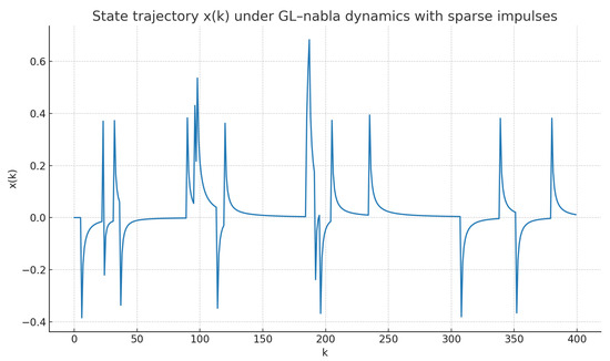
Figure 1. Scenario A (Bernoulli impulses, $p=0.05$): state trajectory $x\left(k\right)$.

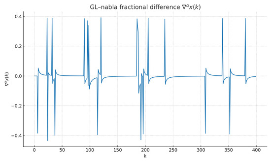
Figure 2. Scenario A: fractional difference ${\nabla }^{\alpha }x\left(k\right)$.

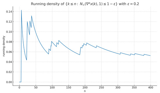
Figure 3. Scenario A: running density of the exceptional set $\{k\le n:N_{\infty }({\nabla }^{\alpha }x\left(k\right),1)\le 1-\epsilon \}$ with $\epsilon =0.2$.

Next, Scenario B (square-time impulses with density $\to 0$) corroborates the density-zero case. Figure 4 presents the state trajectory $x\left(k\right)$. Figure 5 shows the fractional difference ${\nabla }^{\alpha }x\left(k\right)$. Figure 6 demonstrates that the running density of the same exceptional set tends to zero, in line with Proposition 7.

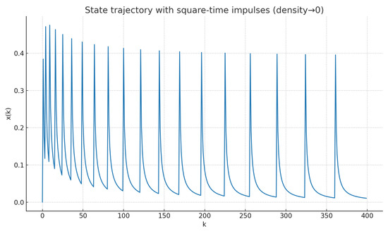
Figure 4. Scenario B (square-time impulses, density $\to 0$): state trajectory $x\left(k\right)$.

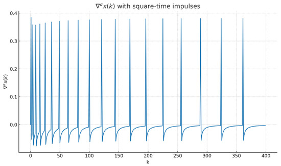
Figure 5. Scenario B: fractional difference ${\nabla }^{\alpha }x\left(k\right)$.

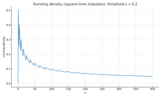
Figure 6. Scenario B: running density $\to 0$ (proof-of-concept for Proposition 7).

Finally, Figure 7 depicts the Grünwald–Letnikov binomial kernel $w_{\alpha }\left(j\right)$ for $\alpha =0.6$, highlighting the long-memory effect via slowly decaying magnitudes and sign alternation.

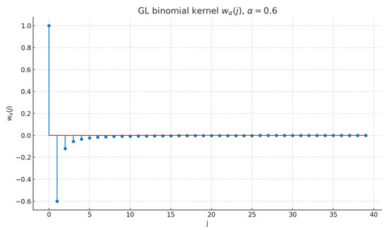
Figure 7. GL binomial kernel $w_{\alpha }\left(j\right)$ for $\alpha =0.6$ (memory effect).

5. Engineering Case Study: Fuzzy Diagnostics for a Fractional Thermal Balance

We demonstrate how the proposed fuzzy statistical framework delivers actionable diagnostics for an engineering-style model: a single-degree thermal balance with memory, time-stepped by the binomial GL nabla operator under imprecise measurements and sparse bursts.

5.1. Model and GL Scheme

Let $x\left(t\right)$ denote a (lumped) temperature state tracking an ambient setpoint u . We evolve x by the binomial GL nabla operator of order $\alpha \in (0,1)$:

$$\left({}_0\nabla ^{\alpha }x\right)\left(t\right)=\lambda \left(u-x\left(t\right)\right)+r\left(t\right),t\in {\mathbb{N}}_0,$$

where $\lambda >0$ is a coupling parameter and $r\left(t\right)$ collects perturbations/measurement errors. Using the binomial representation $\left({}_0\nabla ^{\alpha }x\right)\left(t\right)={\sum }_{j=0}^t{w}_{\alpha }\left(j\right)x(t-j)$ with $w_{\alpha }\left(j\right)={(-1)}^j\left({\displaystyle \genfrac{}{}{0pt}{}{\alpha }{j}}\right)$, solving for $x\left(t\right)$ gives the explicit GL recursion

$$(1+\lambda )x\left(t\right)=\lambda u+r\left(t\right)-{\displaystyle \sum _{j=1}^t}{w}_{\alpha }\left(j\right)x(t-j),t\ge 1,$$

(1)

with $x\left(0\right)$ prescribed. Hence, the memory is realized via a causal binomial convolution.

5.2. Residual-Based Fuzzy Diagnostics

We adopt the Bag–Samanta fuzzy norm induced by the sup-norm, $N_{\infty }(z,t_0)={\displaystyle \frac{t_0}{t_0+\left|z\right|}}$. Given a computed trajectory x , we form the residual

$$\widehat{r}\left(t\right):=\left({}_0\nabla ^{\alpha }x\right)\left(t\right)-\lambda (u-x\left(t\right))={\displaystyle \sum _{j=0}^t}{w}_{\alpha }\left(j\right)x(t-j)-\lambda (u-x\left(t\right)),$$

and evaluate

$$N_{\infty }\left(\widehat{r}\left(t\right),t_0\right)={\displaystyle \frac{t_0}{t_0+\left|\widehat{r}\left(t\right)\right|}}.$$

For fixed $t_0>0$ and $\epsilon \in (0,1)$, call an index t a violation if $N_{\infty }(\widehat{r}\left(t\right),t_0)\le 1-\epsilon$. Our theory is as follows: If the set of violations has natural density 0 then ${\Delta }^{\alpha }$-fuzzy statistical convergence holds (and strong Cesàro ⇒ fuzzy statistical, as in Theorem 9).

5.3. Numerical Experiment (Engineering-Flavored)

We choose $\alpha =0.6$, $\lambda =0.3$, $u=1$, horizon $T=1000$. The perturbation $r\left(t\right)$ combines small zero-mean noise with sparse bursts at square indices $t=n^2$:

$$r\left(t\right)=0.02\xi \left(t\right)+0.5\sigma \left(t\right),\sigma \left(t\right)\in \{-1,0,+1\}\mathrm{and}\sigma \left(t\right)\ne 0\iff t=n^2,$$

where $\xi$ is i.i.d. standard normal. Equation (1) yields $x\left(t\right)$ explicitly. We set $t_0=0.1$, $\epsilon =0.25$.

Findings

Figure 8 shows $x\left(t\right)$ tracking u despite bursts. Figure 9 and Figure 10 depict $|\widehat{r}\left(t\right)|$ and $N_{\infty }(\widehat{r}\left(t\right),t_0)$; bursts create visible spikes yet are sparse. Figure 11 plots the running fraction of violations ${\displaystyle \frac{1}{n}}\left|\{1\le t\le n:N_{\infty }(\widehat{r}\left(t\right),t_0)\le 1-\epsilon \}\right|$, which decays towards 0, confirming the fuzzy statistical smallness of the residuals. Finally, Figure 12 reports the strong Cesàro-type average ${\displaystyle \frac{1}{n}}{\sum }_{t=1}^n(1-N_{\infty }(\widehat{r}\left(t\right),t_0))$, which also tends to 0, aligning with Theorem 9.

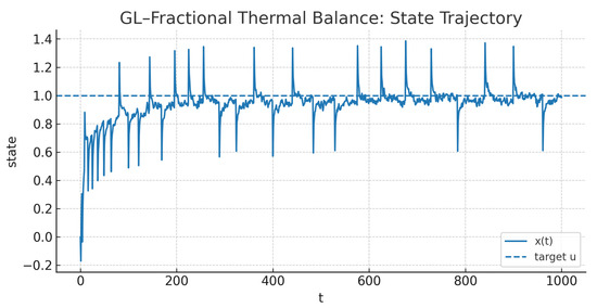
Figure 8. State trajectory under GL memory ($\alpha =0.6$): $x\left(t\right)$ vs. setpoint u . Bursts perturb the path but do not destroy fuzzy statistical convergence.

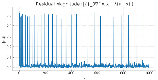
Figure 9. Residual magnitude $|\widehat{r}\left(t\right)|=\left|{}_0\nabla ^{\alpha }x\left(t\right)-\lambda (u-x\left(t\right))\right|$. Sparse bursts appear at $t=n^2$.

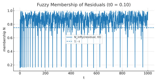
Figure 10. Fuzzy membership of residuals $N_{\infty }(\widehat{r}\left(t\right),t_0)={\displaystyle \frac{t_0}{t_0+\left|\widehat{r}\left(t\right)\right|}}$ with $t_0=0.1$. The dashed line is $1-\epsilon$ with $\epsilon =0.25$.

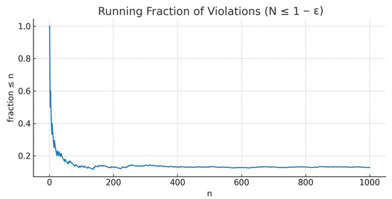
Figure 11. Running fraction of violations $N_{\infty }(\widehat{r}\left(t\right),t_0)\le 1-\epsilon$. Decay towards 0 indicates density-zero violations and, thus, fuzzy statistical convergence.

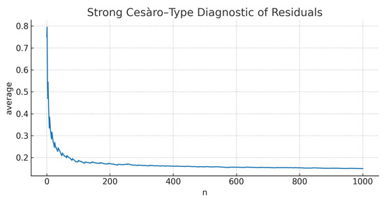
Figure 12. Strong Cesàro-type diagnostic ${\displaystyle \frac{1}{n}}{\sum }_{t=1}^n(1-N_{\infty }(\widehat{r}\left(t\right),t_0))\to 0$, which implies fuzzy statistical convergence (Theorem 9).

5.4. Takeaway for Engineering Practice (Concise Checklist)

Let $\alpha \in (0,1)$, setpoint u , coupling $\lambda >0$, and a computed trajectory $x\left(t\right)$. Define the GL residual

$$\widehat{r}\left(t\right):={}_0\nabla ^{\alpha }x\left(t\right)-\lambda (u-x\left(t\right)),N_{\infty }(z,t_0)={\displaystyle \frac{t_0}{t_0+\left|z\right|}}.$$

Fix resolution $t_0>0$ and threshold $\epsilon \in (0,1)$.

5.4.1. What to Compute

What to compute:

• Membership series $N_{\infty }(\widehat{r}\left(t\right),t_0)$ and the violation set ${\mathcal{V}}_{\epsilon ,t_0}:=\{t:N_{\infty }(\widehat{r}\left(t\right),t_0)\le 1-\epsilon \}$.
• Running density ${\displaystyle D\left(n\right):=\frac{1}{n}|{\mathcal{V}}_{\epsilon ,t_0}\cap \{1,\dots ,n\}|}$.
• (Optional strong mean) ${\displaystyle C\left(n\right):=\frac{1}{n}{\displaystyle \sum _{t=1}^n}\left(1-N_{\infty }(\widehat{r}\left(t\right),t_0)\right)}$.

5.4.2. Decision Rule

Decision rule:

• If $D\left(n\right)\to 0$ as $n\to \infty$ (violations have density 0) then the trajectory is fuzzy statistically robust for the chosen $(t_0,\epsilon )$.
• The auxiliary indicator $C\left(n\right)\to 0$ corroborates this via strong Cesàro ⇒ statistical (Theorem 9).

5.4.3. How to Choose $(t_0,\epsilon )$

How to choose $(t_0,\epsilon )$:

• Set $t_0$ to a robust scale of residuals, e.g., $t_0:=2\mathrm{MAD}\left(\widehat{r}\right)$ (Median Absolute Deviation).
• Take $\epsilon \in [0.1,0.3]$ in practice; smaller $\epsilon$ accepts larger residuals.
• For windowed monitoring, use $\lambda$-density with a sliding window of length ${\lambda }_n$ (e.g., ${\lambda }_n=\lfloor n^{1/2}\rfloor$).

5.4.4. Implementation Notes

Implementation notes:

• Precompute GL weights $w_{\alpha }\left(j\right)={(-1)}^j\left({\displaystyle \genfrac{}{}{0pt}{}{\alpha }{j}}\right)$. For long horizons, truncate at M , such that ${\sum }_{j>M}\left|w_{\alpha }\left(j\right)\right|\le \tau$ (e.g., $\tau ={10}^{-3}$). This yields cost $\mathcal{O}\left(TM\right)$ with negligible loss.
• Right–left forms are equivalent by the discrete reflection Q (Proposition 1); the same diagnostic applies to ${\Delta }_b^{\alpha }$.

5.4.5. Reporting Template

Report $(\alpha ,\lambda ,t_0,\epsilon ,M)$ and the limits ${\lim }_{n\to \infty }D\left(n\right)$, ${\lim }_{n\to \infty }C\left(n\right)$, plus a plot of $D\left(n\right)$. When $D\left(n\right)\to 0$, the residual violations are of natural density zero, which certifies the fuzzy statistical robustness claimed in Section 4.

5.5. Reproducibility Statement

All numerical figures in Section 5 are reproducible with the parameters $(\alpha ,\lambda ,u,T,t_0,\epsilon )=(0.6,0.3,1,1000,0.1,0.25)$. Noise $\xi \left(t\right)$ is standard normal and bursts occur at square indices $t=n^2$ with magnitude $0.5$. A reference implementation (pseudo-code) of the GL recursion (1),

$$(1+\lambda )x\left(t\right)=\lambda u+r\left(t\right)-{\displaystyle \sum _{j=1}^t}{w}_{\alpha }\left(j\right)x(t-j),t\ge 1,$$

A reference implementation sufficient to reproduce the figures is available upon request; any fixed random seed yields qualitatively identical plots.

6. Conclusions

We have introduced and analyzed fuzzy statistical convergence for Grünwald–Letnikov fractional difference sequences in Bag–Samanta fuzzy normed linear spaces. Our contributions include the following: (i) a coherent definition for both nabla-left and delta-right GL operators together with the uniqueness, linearity, and invariance properties of fuzzy statistical limits; (ii) a Cauchy characterization (with the completeness of the underlying fuzzy space ensuring the existence of limits); (iii) an inclusion theory showing that fuzzy strong Cesàro summability—including weighted variants—forces fuzzy statistical convergence; and (iv) a Q-duality principle that transfers all statements between nabla and delta forms, clarifying the GL↔RL correspondence.

On the applied side, we propose density-based residual diagnostics for discrete fractional initial-value problems, and we have illustrated how fuzzy statistically negligible GL-residuals guarantee the robustness of GL-type numerical schemes in the presence of bursty or imprecise data. We have also established a fuzzy Korovkin-type approximation mechanism under GL smoothing: Cesàro-type control on the Korovkin test set implies fuzzy statistical convergence for all targets in $C[a,b]$ equipped with a Bag–Samanta fuzzy norm.

Outlook

Several avenues appear promising: (1) Tauberian theory in fuzzy settings: precise conditions under which fuzzy statistical convergence implies stronger modes of convergence for GL differences. (2) General densities: $\lambda$-densities and lacunary densities for GL operators in fuzzy spaces, with embeddings between the corresponding limit classes. (3) Weighted/variable-order operators: Stability and approximation when the GL order is variable or weights are data-adaptive. (4) Stochastic perturbations: regimes with positive-density impulses and probabilistic bounds for residual-driven diagnostics. (5) Multivariate and space–time grids: extensions to GL-type operators on lattices and graphs, with fuzzy norms tailored to anisotropic resolutions. (6) Numerics under GL schemes. Incorporating sharp pointwise-in-time error bounds and stability insights for GL discretizations into our fuzzy residual tests is a natural next step [16]; see also GL-based iterative solvers and performance evidence in higher-dimensional diffusion problems [17].

We expect these directions to enhance uncertainty-aware analysis and computation for memory-driven models, and to broaden the practical scope of fuzzy diagnostics in fractional difference equations.

References

- Abdeljawad, T. Fractional Sums and Differences with Binomial Coefficients. Discret. Dyn. Nat. Soc. 2013, 2013, 104173. [Google Scholar] [CrossRef]
- Goodrich, C.; Peterson, A.C. Discrete Fractional Calculus; Springer: Cham, Switzerland, 2015. [Google Scholar] [CrossRef]
- Atici, F.M.; Eloe, P.W. Discrete fractional calculus with the nabla operator. Electron. J. Qual. Theory Differ. Equ. 2009, 2009, 12. [Google Scholar] [CrossRef]
- Elaydi, S.N. An Introduction to Difference Equations, 3rd ed.; Springer: New York, NY, USA, 2005. [Google Scholar]
- Bag, T.; Samanta, S.K. Finite Dimensional Fuzzy Normed Linear Spaces. J. Fuzzy Math. 2003, 11, 687–705. [Google Scholar]
- Yan, C. On the Completion of Fuzzy Normed Linear Spaces in the Sense of Bag and Samanta. Fuzzy Inf. Eng. 2021, 13, 236–247. [Google Scholar] [CrossRef]
- Fast, H. Sur la convergence statistique. Colloq. Math. 1951, 2, 241–244. [Google Scholar] [CrossRef]
- Steinhaus, H. Sur la convergence ordinaire et la convergence asymptotique. Colloq. Math. 1951, 2, 73–74. [Google Scholar]
- Baliarsingh, P.; Kadak, U.; Mursaleen, M. On statistical convergence of difference sequences of fractional order and related Korovkin type approximation theorems. Quaest. Math. 2018, 41, 1117–1133. [Google Scholar] [CrossRef]
- Ayman Mursaleen, M.; Serra-Capizzano, S. Statistical Convergence via q-Calculus and a Korovkin’s Type Approximation Theorem. Axioms 2022, 11, 70. [Google Scholar] [CrossRef]
- Tanushri; Ahmad, A.; Esi, A. A Framework for I*-Statistical Convergence of Fuzzy Numbers. Axioms 2024, 13, 639. [Google Scholar] [CrossRef]
- Raj, K.; Gorka, S.; Esi, A. Lacunary Statistical Convergence of Uncertain Fuzzy Number Sequences via Orlicz Function. Math. Found. Comput. 2025, 8, 998–1011. [Google Scholar] [CrossRef]
- Karakaş, A. Statistical convergence of new type difference sequences with Caputo fractional derivative. AIMS Math. 2022, 7, 17091–17104. [Google Scholar] [CrossRef]
- Türkmen, M.R.; Öğünmez, H. I-fp Convergence in Fuzzy Paranormed Spaces. Mathematics 2025, 13, 2478. [Google Scholar] [CrossRef]
- Öğünmez, H.; Türkmen, M.R. Applying λ-Statistical Convergence in Fuzzy Paranormed Spaces to Supply Chain Inventory Management. Mathematics 2025, 13, 1977. [Google Scholar] [CrossRef]
- Chen, H.; Jiang, Y.; Wang, J. Grünwald–Letnikov scheme for a multi-term time fractional reaction-subdiffusion equation. Commun. Nonlinear Sci. Numer. Simul. 2024, 132, 107930. [Google Scholar] [CrossRef]
- Kittisopaporn, A.; Chansangiam, P. Approximate solutions of the 2D space-time fractional diffusion equation via a gradient-descent iterative algorithm with Grünwald–Letnikov approximation. AIMS Math. 2022, 7, 8471–8490. [Google Scholar] [CrossRef]
- Ortigueira, M.D. Discrete-Time Fractional Difference Calculus: Origins, Evolutions and New Formalisms. Fractal Fract. 2023, 7, 502. [Google Scholar] [CrossRef]
- Fang, J.X. On I-topology generated by fuzzy norm. Fuzzy Sets Syst. 2006, 157, 2739–2750. [Google Scholar] [CrossRef]
- Şencimen, C.; Pehlivan, I. Statistical convergence in fuzzy normed linear spaces. Fuzzy Sets Syst. 2008, 159, 361–370. [Google Scholar] [CrossRef]
- Kizmaz, H. On Certain Sequence Spaces. Can. Math. Bull. 1981, 24, 169–176. [Google Scholar] [CrossRef]
- Baliarsingh, P. Some new difference sequence spaces of fractional order and their dual spaces. Appl. Math. Comput. 2013, 219, 9737–9742. [Google Scholar] [CrossRef]
- Ercan, S. Some Cesàro-Type Summability and Statistical Convergence of Sequences Generated by Fractional Difference Operator. Afyon Kocatepe Univ. J. Sci. Eng. 2018, 18, 125–130. [Google Scholar] [CrossRef]
Disclaimer/Publisher’s Note: The statements, opinions and data contained in all publications are solely those of the individual author(s) and contributor(s) and not of MDPI and/or the editor(s). MDPI and/or the editor(s) disclaim responsibility for any injury to people or property resulting from any ideas, methods, instructions or products referred to in the content. |
© 2025 by the authors. Licensee MDPI, Basel, Switzerland. This article is an open access article distributed under the terms and conditions of the Creative Commons Attribution (CC BY) license (https://creativecommons.org/licenses/by/4.0/).