Four-Step T-Stable Generalized Iterative Technique with Improved Convergence and Various Applications

Abstract

This research presents a new form of iterative technique for Garcia-Falset mapping that outperforms previous iterative methods for contraction mappings. We illustrate this fact through comparison and present the findings graphically. The research also investigates convergence of the new iteration in uniformly convex Banach space and explores its stability. To further support our findings, we present its working on to a BV problem and to a delay DE. Finally, we propose a design of an implicit neural network that can be considered as an extension of a traditional feed forward network.

1. Introduction

The theory of fixed points (FP) is a discipline that studies the criteria for the existence and uniqueness of FPs for specific mappings in abstract spaces. This theory, built on the basis of the Banach contraction principle (BCP), demonstrates that the FP of contraction mapping is unique in the entire metric space. In the early 1900s, scholars expanded the BCP to the encompass multiple abstract spaces and developed additional types of contraction mapping. Initially, the notion of fixed points focused solely on locating them. However, in other cases, it is impossible to determine fixed points using direct approaches, particularly for nonlinear mapping. As a result, iterative approximations are offered as an alternative method for estimating the fixed point. Many issues in applied physics and engineering are too complex to solve with traditional analytical approaches [1,2,3,4,5]. In such instances, FP theory proposes several alternate strategies for obtaining the desired results. To begin, we convert the problem to an FP problem, ensuring that the FP set of one problem is equivalent to the solution set of the other. This establishes that the existence of a FP for an equation implies the existence of a solution for it. Suppose $\mathbb{N}$ and $\mathbb{R}$ represent the standard notations for the set. Consider $C\ne \varnothing$ to be a closed convex subset of a uniformly convex Banach space (UCBS). $T:C\to C$ represents a contraction ( resp., nonexpansive) mapping if there is a constant $H\in [0,1)$ (resp., $H=1$) that satisfies:

$$∥Tx-Ty∥\le H∥x-y∥$$

for all $x,y\in C$. The set of FP of T is denoted by $F\left(T\right)$.

In 1965, refs [6,7,8] developed FP theorem for nonexpansive mappings in a UCBS. A Banach space S is uniformly convex if for any $ϵ>0$, some $\delta >0$ exists such that $∥x+y∥\le 2(1-\delta )$ holds whenever $∥x∥\le 1$, $∥y∥\le 1$ and $∥x-y∥\ge ϵ$. Soon after, Goebel [9] established a basic proof for the Kirk–Browder–Gohde Theorem. Several writers have explained that nonexpansive mappings occur spontaneously while studying nonlinear problems in various distance space topologies. Thus, it is entirely reasonable to investigate extensions of these mappings.

BCP ensures the uniqueness of FP for every contraction T on a Banach space. A similar claim for nonexpansive mapping is no longer accurate.

Additionally, even if a nonexpansive T has a FP which is unique, the Picard iteration $x_n=T^n{x}_0$ may not be useful to find it.

Thanks to these aspects, nonexpansive mappings have been a significant research topic in nonlinear analysis. In 2008, Suzuki [10] extended nonexpansive mappings by defining it with a weaker inequality. A self-map $T:C\to C$ is defined to satisfy condition (C), if $∥Tx-Ty∥\le ∥x-y∥$ holds for each $x,y\in C$ whenever:

$$\begin{array}{c}\hfill {\displaystyle \frac{1}{2}}∥x-Tx∥\le ∥x-y∥.\end{array}$$

(1)

It seems trivial that a nonexpansive mapping satisfies condition (C), but [10] demonstrated with an example that the converse does not generally hold true. Thus, Suzuki mappings have a broader class as compared to the nonexpansive mappings. On similar lines, Garcia-Falset et al. [11] established a new class that is more general than the class of Suzuki (C) and can be defined as follows:

$T:C\to C$ is a Garcia-Falset map (or a map T with condition (E)) if there is $\mu \le 1$ for $x,y\in C$ such that:

$$\begin{array}{c}\hfill ∥x-Ty∥\le \mu ∥x-Tx∥+∥x-y∥.\end{array}$$

(2)

It is trivial to verify that every Suzuki mapping T satisfies condition (E) with $\mu =3$. We now present an example for a map $T:C\to C$, with condition (E), and show that it is not nonexpansive.

Example 1.

Consider $C=[2,7]$ a self-map $T:C\to C$ is defined by:

$$Tx=\left\{\begin{array}{c}{\displaystyle \frac{2x+5}{3}},ifx\in C_1=[0,7)\hfill \\ \\ 5,ifx\in C_2=\left\{7\right\}.\hfill \end{array}\right.$$

To verify that T satisfies condition (E), we need to check

$$∥x-Ty∥\le \mu ∥x-Tx∥+∥x-y∥,$$

for some $\mu \ge 1$ and $\forall x,y\in C$.

Fixing the value of $\mu =4$, we discuss the following cases. $\left(M_1\right)$: Select $x,y\in C_2$, then $Tx=5=Ty$. We have:

$$\begin{array}{ccc}\hfill ∥x-Ty∥& =& |x-Ty|\hfill \\ & =& |x-5|\hfill \\ & =& |x-Tx|\hfill \\ & \le & 4|x-Tx|+|x-y|\hfill \\ & =& 4\left|\right|x-Tx\left|\right|+\left|\right|x-y\left|\right|.\hfill \end{array}$$

(3)

$\left(M_2\right)$: Choose any $x,y\in C_1$, then $Tx={\displaystyle \frac{2x+5}{3}}$ and $Ty={\displaystyle \frac{2y+5}{3}}$. We have:

$$\begin{array}{ccc}\hfill ∥x-Ty∥& =& |x-Ty|\hfill \\ & \le & |x-Tx|+|Tx-Ty|\hfill \\ & =& |x-Tx|+|{\displaystyle \frac{2x}{3}}-{\displaystyle \frac{2y}{3}}|\hfill \\ & =& |x-Tx|+{\displaystyle \frac{2}{3}}|x-y|\hfill \\ & \le & |x-Tx|+|x-y|\hfill \\ & \le & 4|x-Tx|+|x-y|\hfill \\ & =& 4\left|\right|x-Tx\left|\right|+\left|\right|x-y\left|\right|.\hfill \end{array}$$

$\left(M_3\right)$: Choose any $x\in \left(C_1\right)$ and $y\in C_2$, then $Tx={\displaystyle \frac{2x+5}{3}}$ and $Ty=5$. We have:

$$\begin{array}{ccc}\hfill ∥x-Ty∥& =& |x-Ty|\hfill \\ & =& |x-5|\hfill \\ & =& 3|{\displaystyle \frac{x-5}{3}}|\hfill \\ & =& 3|x-{\displaystyle \frac{2x+5}{3}}|\hfill \\ & =& 3|x-Tx|\hfill \\ & \le & 4|x-Tx|\hfill \\ & \le & 4|x-Tx|+|x-y|\hfill \\ & =& 4\left|\right|x-Tx\left|\right|+\left|\right|x-y\left|\right|.\hfill \end{array}$$

$\left(M_4\right)$: Choose any $x\in \left(C_2\right)$ and $y\in C_1$, then $Tx=5$ and $Ty={\displaystyle \frac{2x+5}{3}}$. We have:

$$\begin{array}{ccc}\hfill ∥x-Ty∥& =& |x-Ty|\hfill \\ & =& |x-{\displaystyle \frac{2y+5}{3}}|\hfill \\ & =& |{\displaystyle \frac{3x-2y-5}{3}}|\hfill \\ & =& |{\displaystyle \frac{2x+x-2y-5}{3}}|\hfill \\ & \le & |{\displaystyle \frac{2(x-y)}{3}}|+|{\displaystyle \frac{x-5}{3}}|\hfill \\ & =& {\displaystyle \frac{2}{3}}|x-y|+{\displaystyle \frac{1}{3}}|x-5|\hfill \\ & \le & |x-Tx|+|x-y|\hfill \\ & \le & 4|x-Tx|+|x-y|\hfill \\ & =& 4\left|\right|x-Tx\left|\right|+\left|\right|x-y\left|\right|.\hfill \end{array}$$

In the above, we proved that in each case T satisfies condition (E). When choosing $x=6.5$ and $y=7$ and fixed point of this is $p=5$, it is easily can be seen that $1=\left|\right|Tx-Ty\left|\right|>\left|\right|x-y\left|\right|=0.5$ but $1=\left|\right|Tx-Tp\left|\right|<\left|\right|x-p\left|\right|=1.5$. Hence, $T:C\to C$ is a Garcia-Falset mapping.

Remark 1.

Every Garcia-Falset mapping is not a nonexpansive mapping.

Soon after this discovery for these mappings, the approximation of FP under Ishikawa iteration in a certain-distance space was first studied by Bagherboum [12].

Iterative Techniques

Iterative techniques can solve a variety of issues, including minimization, equilibrium, and viscosity approximation in various domains [13,14,15,16]. Picard [17] proposed an iterative scheme for approximation of the FP in 1890 as follows:

$$\begin{array}{c}\hfill \left\{\begin{array}{cc}{x}_1\hfill & =x\in C\hfill \\ x_{n+1}\hfill & =T{x}_n,n\in \mathbb{N}\hfill \end{array}\right.\end{array}$$

(4)

Some well-known iteration processes that are often used to approximate FPs of nonexpansive mappings include Picard [17], Mann [18], Ishikawa [19], Noor [20], Abbas and Nazir [21] and Thakur et al. [22] iterations. A Thakur iteration [22] is as follows:

$$\begin{array}{c}\hfill \left\{\begin{array}{cc}{x}_{n+1}\hfill & =(1-M_n)T{z}_n+M_{n}T{y}_n\hfill \\ y_n\hfill & =T((1-N_n)z_n+N_{n}T{z}_n)\hfill \\ z_n\hfill & =T((1-O_n)x_n+O_{n}T{x}_n),n\in \mathbb{N}\hfill \end{array}\right.\end{array}$$

(5)

where $\left\{M_n\right\}$, $\left\{N_n\right\}$ and $\left\{O_n\right\}$ are in (0, 1). They established that, for contractive mappings, it converges faster than iterations of [17,18,19,20,21].

The Asghar Rahim iteration [23] is as follows:

$$\begin{array}{c}\hfill \left\{\begin{array}{cc}{x}_{n+1}\hfill & =(1-M_n)T{y}_n+M_{n}T{z}_n\hfill \\ y_n\hfill & =T((1-N_n)x_n+N_n{z}_n)\hfill \\ z_n\hfill & =T((1-O_n)x_n+O_{n}T{x}_n),n\in \mathbb{N}\hfill \end{array}\right.\end{array}$$

(6)

where $\left\{M_n\right\}$, $\left\{N_n\right\}$ and $\left\{O_n\right\}$ are in (0, 1). This process also proven by the authors to be faster than that of [17,18,19,20,21,22].

A Picard–Thakur hybrid iteration [12] is as follows:

$$\begin{array}{c}\hfill \left\{\begin{array}{cc}{j}_{n+1}\hfill & =V{k}_n\hfill \\ k_n\hfill & =(1-M_n)V{m}_n+M_{n}V{l}_n\hfill \\ l_n\hfill & =(1-N_n)m_n+N_{n}V{m}_n\hfill \\ m_n\hfill & =(1-O_n)j_n+O_{n}V{j}_n,n\in \mathbb{N}\hfill \end{array}\right.\end{array}$$

(7)

where $\left\{M_n\right\}$, $\left\{N_n\right\}$ and $\left\{O_n\right\}$ are in (0, 1). They proved that this process converges faster than iteration processes (4)–(6) for contraction mappings.

Akanimo iteration [24] is as follows:

$$\begin{array}{c}\hfill \left\{\begin{array}{cc}{x}_{n+1}\hfill & =(1-M_n)T{z}_n+M_{n}T{y}_n\hfill \\ y_n\hfill & =T\left(T{z}_n\right)\hfill \\ z_n\hfill & =T((1-N_n)x_n+N_{n}T{x}_n),n\in \mathbb{N}\hfill \end{array}\right.\end{array}$$

(8)

where $\left\{M_n\right\}$, $\left\{N_n\right\}$ are in (0, 1). They proved that it converges faster than iterations (4)–(7) for contractive mappings.

Iterative methods based on fixed-point theory are essential in order to solve the heat equation.

Time delays add complexity to delay differential equations, which is why fixed-point iterative techniques (4)–(7) are employed. By approximating the system’s state at each time step, these methods iteratively approach a solution, aiding in the stabilization and precise solution of equations when delays impact future behavior.

Implicit neural networks can be regarded as extensions of feedforward neural networks that allow for the transfer of training parameters between layers through input-injected weight tying. In fact, backpropagation in implicit networks is achieved by implicit differentiation in gradient computation, while evaluation of function is carried out by solving a FP equation. Compared to typical neural networks, implicit models have better memory efficiency and greater flexibility because of these special characteristics. However, because their FP equations are nonlinear, implicit networks may experience instability during training.

The fact that deep learning models are very effective when equipped with implicit layers has been demonstrated by numerous publications in learning theory. These learning models substitute a rule of composition, which may be a fixed-point scheme or a differential equation solution for the concept of layers. Known deep learning frameworks that use implicit infinite-depth layers are neural ODEs [25], implicit deep learning [26] and deep equilibrium networks [27]. In [28], the convergence of specific classes of implicit networks to global minima is examined.

The research of implicit-depth learning models’ well-posedness and numerical stability has attracted attention lately. An adequate spectral requirement for the convergence and well-posedness of the Picard’s scheme, connected to the implicit network fixed-point equation, is presented by [26].

Robust and well-posed implicit neural networks for the non-Euclidean norm $l_{\infty }$ are built on the basis of contraction theory [29]. In order to create durable models, they develop a training problem that is constrained by the average iteration and the well-posedness condition. The input–output Lipschitz constant is used as a regularizer in this process. A new kind of deep learning model that works on the basis of implicit prediction rules is presented in [26]. These principles are unlike modern neural networks as they are not produced through a recursive approach across multiple layers. Instead, they rely on solving a fixed-point problem in a “state” vector $x\in R^n$.

The structure of the paper is as follows. First, we present a novel iterative technique for Garcia-Falset mapping and evaluate its convergence and stability in UCBS. Secondly, we compare this with different well-known iterative schemes, and finally, we illustrate its applications in various problems, namely the BV problem, delay DE and a training problem for an implicit neural network.

2. Rate of Convergence

In this paper, we prove that our novel iterative scheme converges faster than iteration processes (4)–(6). Our novel proposed iteration is given by:

$$\begin{array}{c}\hfill \left\{\begin{array}{cc}{x}_{n+1}\hfill & =T\left(T\left(p_n\right)\right)\hfill \\ p_n\hfill & =T((1-M_n)T{z}_n+M_{n}T{y}_n)\hfill \\ y_n\hfill & =T((1-N_n)x_n+N_{n}T{z}_n)\hfill \\ z_n\hfill & =T((1-O_n)x_n+O_{n}T{x}_n),n\in \mathbb{N}\hfill \end{array}\right.\end{array}$$

(9)

where $\left\{M_n\right\}$, $\left\{N_n\right\}$ and $\left\{O_n\right\}$ are in (0,1).

Theorem 1.

Let $C\ne \varnothing$ be a closed and convex subset of a UCBS. Let T be a contraction mapping with some constant $H\in (0,1)$ and fixed point p. Let $\left\{u_n\right\}$ be defined by (6) and $\left\{x_n\right\}$ by (9), where {$M_n$}, {$N_n$}, {$O_n$} are sequences in [ϵ, 1 $-ϵ$] for every $n\in \mathbb{N}$ and some $ϵ\in (0,1)$. Then, the rate of convergence of $\left\{x_n\right\}$ is greater than the rate of $\left\{u_n\right\}$.

Proof. 

As proven in Theorem 2 of [23], we have:

$$∥u_{n+1}-p∥\le H^n{[1-(1-H)NO)]}^n.$$

(10)

Let

$$u_n=H^n{[1-(1-H)NO]}^n∥u_1-p∥.$$

(11)

Using the iterative scheme (9), we have:

$$\begin{array}{ccc}\hfill ∥z_n-p∥& =& \left|\right|T[(1-O_n)x_n+O_{n}T{x}_n]-p\left|\right|\hfill \\ & \le & H\left|\right|(1-O_n)(x_n-p)+O_n(T{x}_n-p)\left|\right|\hfill \\ & \le & H[(1-O_n)∥x_n-p∥+O_n∥T{x}_n-p∥]\hfill \\ & \le & H[(1-O_n)∥x_n-p∥+O_{n}H∥x_n-p∥]\hfill \\ & =& H[1-(1-H)O_n]∥x_n-p∥\hfill \end{array}$$

so that

$$\begin{array}{ccc}\hfill ∥y_n-p∥& =& \left|\right|T[(1-N_n)z_n+N_{n}T{z}_n]-p\left|\right|\hfill \\ & \le & H\left|\right|(1-N_n)(z_n-p)+N_n(T{z}_n-p)\left|\right|\hfill \\ & \le & H[(1-N_n)∥z_n-p∥+N_n∥T{z}_n-p∥]\hfill \\ & \le & H[(1-N_n)∥z_n-p∥+N_{n}H∥z_n-p∥]\hfill \\ & =& H[1-(1-H)N_n]∥z_n-p∥\hfill \\ & <& H(1-(1-H)N_n)(1-(1-H)O_n)∥x_n-p∥\hfill \end{array}$$

and

$$\begin{array}{ccc}\hfill ∥p_n-p∥& =& \left|\right|T[(1-M_n)T{z}_n+M_{n}T{y}_n]-p\left|\right|\hfill \\ & \le & H\left|\right|(1-M_n)(T{z}_n-p)+M_n(T{y}_n-p)\left|\right|\hfill \\ & \le & H[(1-M_n)∥T{z}_n-p∥+M_n∥T{y}_n-p∥]\hfill \\ & \le & H[(1-M_n)H∥z_n-p∥+M_{n}H∥y_n-p∥]\hfill \\ & \le & H[(1-M_n)H^2(1-(1-H)O_n)∥x_n-p∥\hfill \\ & & +M_n{H}^2(1-(1-H)O_n)(1-(1-H)N_n)∥x_n-p∥]\hfill \\ & \le & H^3(1-(1-H)O_n)[(1-M_n)+M_n(1-(1-H))N_n]∥x_n-p∥\hfill \\ & =& H^3(1-(1-H)O_n)\left[(1-(1-H))N_n\right]∥x_n-p∥\hfill \\ & =& H^3[1-(1-H)M_n{N}_n-(1-H)O_n+{(1-H)}^2{O}_n{N}_n{M}_n]∥x_n-p∥\hfill \\ & \le & H^3[1-(1-H)M_n{N}_n-(1-H)O_n+(1-H)O_n{N}_n{M}_n]∥x_n-p∥\hfill \\ & \le & H^3[1-(1-H)(M_n{N}_n+O_n-O_n{N}_n{M}_n]∥x_n-p∥\hfill \\ & <& H[1-(1-H)(M_n{N}_n+O_n-O_n{N}_n{M}_n]∥x_n-p∥.\hfill \end{array}$$

Thus,

$$\begin{array}{ccc}\hfill ∥x_{n+1}-p∥& =& ∥T\left(T{P}_n\right)-p∥\hfill \\ & \le & H∥T{p}_n-p∥\hfill \\ & \le & H^2∥p_n-p∥\hfill \\ & \le & H^3[1-(1-H)(M_n{N}_n+O_n-O_n{N}_n{M}_n]∥x_n-p∥.\hfill \end{array}$$

(12)

Let

$$\begin{array}{ccc}\hfill b_n& =& H^{3n}[1-(1-H){(M_n{N}_n+O_n-O_n{N}_n{M}_n]}^n∥x_1-p∥.\hfill \end{array}$$

Then,

$$\begin{array}{ccc}\hfill {\displaystyle \frac{b_n}{u_n}}& =& {\displaystyle \frac{H^{3n}[1-(1-H){(M_n{N}_n+O_n-k{O}_n{N}_n{M}_n]}^n∥x_1-p∥}{H^n{[1-(1-H)NO]}^n∥u_1-p∥}}\hfill \\ & =& {\displaystyle \frac{H^3[1-(1-H){(M_n{N}_n+O_n-O_n{N}_n{M}_n]}^n∥x_1-p∥}{H^n{[1-(1-H)NO]}^n∥u_1-p∥}}\to 0n\to \infty .\hfill \end{array}$$

(13)

From Definition 3.4 of [30], $\left\{x_n\right\}$ converges faster than $\left\{u_n\right\}$. □

Remark 2.

As proven in [31], Thakur iteration (5) is faster than Ishikawa [19], Noor [20], Abbas and Nazir [21]. So, we will compare our proposed iteration with Picard (4), Thakur (5) and Asghar Rahimi (6).

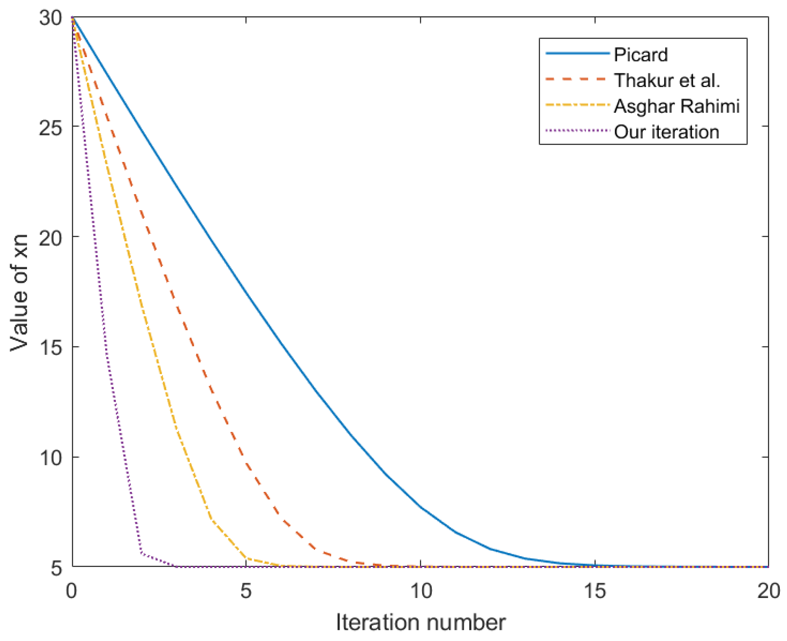
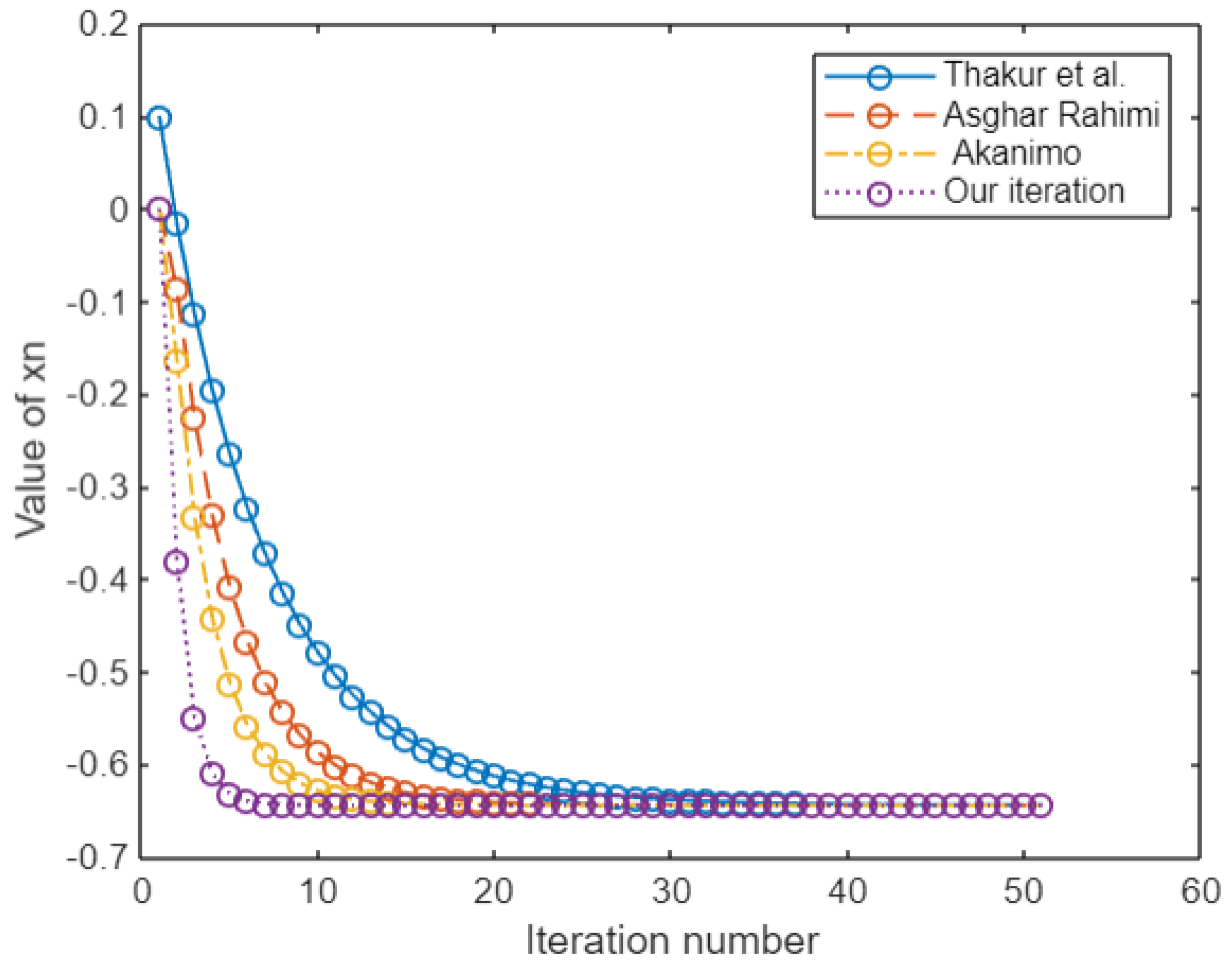
We now demonstrate with an example that our novel iteration (9) converges at a greater rate than Picard (4), Thakur (5) and Asghar Rahimi iteration processes (6).

Example 2.

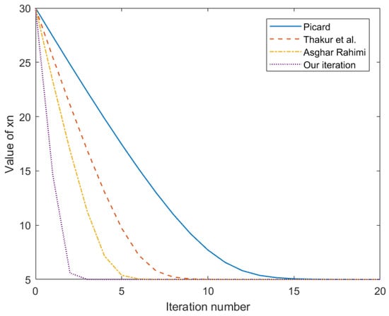
Consider $T:\mathbb{R}\to \mathbb{R}$ to be a mapping defined by $T\left(x\right)=\sqrt{x^2-6x+30}$ for any $x\in \mathbb{R}$. Choose $M_n=N_n=O_n={\displaystyle \frac{1}{2}}$, with an initial guess $x_1=30$. It can be easily seen that $x=5$ is a fixed point of T. Table 1 and Figure 1 below shows the comparison of all the iterative schemes to a fixed point of T in 21 iterations.

Table 1. Comparing iteration convergence.

No. of Iterations	Picard	Thakur	Asghar Rahimi	New Iteration
1	30	30	30	30
2	27.3861278753	25.4605027258	23.2381722116	14.6168424629
3	24.8129650132	21.0691659384	16.8793944946	5.5974190240
4	22.2891328380	16.8924163440	11.2697340648	5.0032637416
5	19.8260093221	13.0431036573	7.1650814763	5.0000149868
6	17.4388815498	9.7163929865	5.3849641099	5.0000000688
7	15.1486402165	7.2125863864	5.0454052746	5.0000000003
8	12.9842003647	5.7772680541	5.0049230360	5.0000000000
9	10.9856386670	5.2154250367	5.0005284002	5.0000000000
10	9.2070855823	5.0535678237	5.0000566520	5.0000000000
11	7.7154333272	5.0128902394	5.0000060732	5.0000000000
12	6.5753563754	5.0030760332	5.0000006510	5.0000000000
13	5.8123294135	5.0007325602	5.0000000698	5.0000000000
14	5.3767273252	5.0001743757	5.0000000075	5.0000000000
15	5.1622507474	5.0000415029	5.0000000008	5.0000000000
16	5.0670828190	5.0000098778	5.0000000001	5.0000000000
17	5.0272091045	5.0000023509	5.0000000000	5.0000000000
18	5.0109456945	5.0000005595	5.0000000000	5.0000000000
19	5.0043883329	5.0000001332	5.0000000000	5.0000000000
20	5.0017569502	5.0000000317	5.0000000000	5.0000000000
21	5.0007030393	5.0000000075	5.0000000000	5.0000000000

Figure 1. Convergence rate of iterative schemes [22].

3. Convergence Results for Garcia-Falset Mapping

Lemma 1.

Let $\varnothing \ne C$ be a convex and closed subset of a Banach space S and $T:C\to C$ is a mapping with condition (E). If $x_n$ defined by (9) then ${lim}_{n\to \infty }∥x_n-p∥$ exists for every fixed point p provided that $F\left(T\right)\ne \varnothing$.

Proof. 

Recall that $F\left(T\right)\ne \varnothing$. By Lemma 6 of [10], we have:

$$\begin{array}{ccc}\hfill ∥z_n-p∥& =& \left|\right|T[(1-O_n)x_n+O_{n}T{x}_n]-p\left|\right|\hfill \\ & \le & \left|\right|(1-O_n)(x_n-p)+O_n(T{x}_n-p)\left|\right|\hfill \\ & \le & [(1-O_n)∥x_n-p∥+O_n∥T{x}_n-p∥]\hfill \\ & \le & [(1-O_n)∥x_n-p∥+O_n∥x_n-p∥]\hfill \\ & =& ∥x_n-p∥\hfill \end{array}$$

(14)

so that

$$\begin{array}{ccc}\hfill ∥y_n-p∥& =& \left|\right|T[(1-N_n)z_n+N_{n}T{z}_n]-p\left|\right|\hfill \\ & \le & \left|\right|(1-N_n)(z_n-p)+N_n(T{z}_n-p)\left|\right|\hfill \\ & \le & [(1-N_n)∥z_n-p∥+N_n∥T{z}_n-p∥]\hfill \\ & \le & [(1-N_n)∥z_n-p∥+N_n∥z_n-p∥]\hfill \\ & =& ∥z_n-p∥\hfill \\ & <& ∥x_n-p∥\hfill \end{array}$$

(15)

and

$$\begin{array}{ccc}\hfill ∥p_n-p∥& =& \left|\right|T[(1-M_n)T{z}_n+M_{n}T{y}_n]-p\left|\right|\hfill \\ & \le & \left|\right|(1-M_n)(T{z}_n-p)+M_n(T{y}_n-p)\left|\right|\hfill \\ & \le & [(1-M_n)∥T{z}_n-p∥+M_n∥T{y}_n-p∥]\hfill \\ & \le & [(1-M_n)∥z_n-p∥+M_n∥y_n-p∥]\hfill \\ & \le & [(1-M_n)∥x_n-p∥+M_n∥x_n-p∥]\hfill \\ & =& ∥x_n-p∥.\hfill \end{array}$$

(16)

Thus,

$$\begin{array}{ccc}\hfill ∥x_{n+1}-p∥& =& ∥T\left(p_n\right)-p∥\hfill \\ & \le & ∥p_n-p∥\hfill \\ & \le & ∥T{p}_n-p∥\hfill \\ & \le & ∥x_n-p∥\hfill \end{array}$$

(17)

Hence, $∥x_n-p∥$ is bounded and nonincreasing for every $p\in F\left(T\right)$. Thus, ${lim}_{n\to \infty }∥x_n-p∥$ exists. □

Lemma 2.

Let $\varnothing \ne C$ be a convex and closed subset of a Banach space S and $T:C\to C$ be a Garcia-Falset mapping. Suppose $x_n$ is defined by (9) and $F\left(T\right)\ne \varnothing$, then

${lim}_{n\to \infty }∥T{x}_n-x_n∥=0$.

Proof. 

From Lemma 1, for each $\mathit{p}\in F\left(T\right)$, ${lim}_{n\to \infty }∥x_n-p∥$ exists. Suppose that there exists $t\ge 0$, such that:

$$\begin{array}{ccc}\hfill \underset{n\to \infty }{lim}∥x_n-p∥& =& t\hfill \end{array}$$

(18)

From the proof of Lemma 1 we obtain that $∥z_n-p∥\le ∥x_n-p∥$. Accordingly, one has

$$\begin{array}{ccc}\hfill \underset{n\to \infty }{lim}sup∥z_n-p∥\le \underset{n\to \infty }{lim}sup∥x_n-p∥& =& t\hfill \end{array}$$

(19)

Now p is the fixed point, and by Lemma 6 of [10], we obtain that $∥T{x}_n-p∥\le ∥x_n-p∥$

$$\begin{array}{ccc}\hfill \underset{n\to \infty }{lim}sup∥T{x}_n-p∥\le \underset{n\to \infty }{lim}sup∥x_n-p∥& =& t\hfill \end{array}$$

(20)

Again, by the proof of Lemma 1, we obtain that $∥y_n-p∥\le ∥z_n-p∥$. So,

$$∥x_{n+1}-p∥\le [(1-M_n)∥x_n-p∥+M_n∥y_n-p∥]$$

$$\le [(1-M_n)∥x_n-p∥+M_n∥z_n-p∥]$$

Hence,

$$∥x_{n+1}-p∥-∥x_n-p∥\le {\displaystyle \frac{∥x_{n+}-p∥-∥x_n-p∥}{M_n}}\le ∥z_n-p∥-∥x_n-p∥.$$

So,

$$∥x_{n+1}-p∥\le ∥z_n-p∥.$$

From (18), we have

$$\begin{array}{ccc}\hfill t& \le & \underset{n\to \infty }{lim}inf∥z_n-p∥.\hfill \end{array}$$

(21)

Hence, from (19) and (21), we have

$$t=\underset{n\to \infty }{lim}∥z_n-p∥$$

From (9) and from (18), we have

$$\begin{array}{ccc}\hfill t& =& \underset{n\to \infty }{lim}∥z_n-p∥\hfill \\ & =& \underset{n\to \infty }{lim}\left|\right|T[(1-O_n)x_n+O_{n}T{x}_n]-p\left|\right|\hfill \\ & \le & \underset{n\to \infty }{lim}\left|\right|(1-O_n)({\mathit{x}}_n-p)+O_n(T{x}_n-p)\left|\right|\hfill \\ & \le & \underset{n\to \infty }{lim}[(1-O_n)∥x_n-p∥+\underset{n\to \infty }{lim}{O}_n∥T{x}_n-p∥]\hfill \\ & \le & t.\hfill \end{array}$$

(22)

Hence,

$$t=\underset{n\to \infty }{lim}\left|\right|(1-O_n)(x_n-p)+O_n(T{x}_n-p)\left|\right|$$

Now, from (19), (20), (22) and Lemma 2.5 of [30], ${lim}_{n\to \infty }∥T{x}_n-x_n∥=0$. □

4. Stability

In this section, we establish the stability for Garcia-Falset mappings via our novel iteration process (9).

Theorem 2.

The iterative process $\left\{x_n\right\}$ defined by Equation (9) is T-stable in the sense of Harder and Hicks [32].

Proof. 

Suppose $u_n$ is an arbitrary sequence in C and $u_{n+1}=f(T,u_n)$ is the sequence generated by (9) converging to a fixed point p (by Theorem 1) and ${\delta }_n=∥u_{n+1}-f(T,u_n)∥$ for all $n\in \mathbb{Z}+$. We have to prove that ${lim}_{n\to \infty }{\delta }_n=0$ which implies that ${lim}_{n\to \infty }{u}_n=p$. Suppose ${lim}_{n\to \infty }{\delta }_n=0$; then, by iteration process (9), we have

$$\begin{array}{ccc}\hfill ∥u_{n+1}-p∥& \le & ∥u_{n+1}-f(T,u_n)∥+∥f(T,u_n)-p∥\hfill \\ & \le & {\delta }_n+∥f(T,u_n)-p∥\hfill \\ & \le & {\delta }_n+H^3[1-(1-H)(M_n{N}_n+O_n-O_n{N}_n{M}_n]∥u_n-p∥.\hfill \end{array}$$

(23)

since

$$\begin{array}{ccc}\hfill 0<(1-(1-H)\left(M_n{N}_n\right))& \le & 1,\hfill \end{array}$$

and

$$\begin{array}{ccc}\hfill 0<(1-(1-H)(M_n{N}_n+O_n-O_n{N}_n{M}_n)& \le & 1,\hfill \end{array}$$

we obtain $∥u_{n+1}-p∥\le {\delta }_n+H^3∥u_n-p∥$.

Define $v_n=∥u_n-p∥$. Then, $u_{n+1}\le H^3{v}_n+{\delta }_n$. Since ${lim}_{n\to \infty }{\delta }_n=0$, we have ${lim}_{n\to \infty }{v}_n=0$, i.e., ${lim}_{n\to \infty }{u}_n=p$. Conversely, suppose ${lim}_{n\to \infty }{u}_n=p$, we have:

$$\begin{array}{ccc}\hfill {\delta }_n& =& ∥u_{n+1}-f(T,u_n)∥\hfill \\ & \le & ∥u_{n+1}-p∥+∥f(T,u_n)-p∥\hfill \\ & \le & ∥u_{n+1}-p∥+H^3[1-(1-H)(M_n{N}_n+O_n-O_n{N}_n{M}_n]∥u_n-p∥\hfill \\ & \le & ∥u_{n+1}-\mathit{p}∥+H^3∥u_n-p∥\hfill \end{array}$$

This implies that ${lim}_{n\to \infty }{\delta }_n=0$. Hence, iteration process (9) is T-stable. □

5. Application

Thermal analysis and engineering both make extensive use of the heat equation, which represents the temperature distribution over time in a specific location. By adding delays, delay differential equations expand on conventional differential equations and can be used in systems where past states affect future behavior, such as population dynamics. Implicit functions are used by designed implicit neural networks to define outputs, resulting in reliable and effective solutions to challenging issues.

5.1. Heat Equation

Consider the following one-dimensional heat equation:

$$\begin{array}{c}\hfill {\displaystyle \frac{\partial u}{\partial t}}=\alpha {\displaystyle \frac{{\partial }^{2}u}{\partial x^2}},0<x<L,0<t<\infty ,\end{array}$$

(24)

The initial and homogeneous boundary conditions are given as follows:

$$u(x,0)=f\left(x\right),$$

(25)

and

$$u(0,t)=0\mathrm{and}u(L,t)=0,$$

(26)

$f\left(x\right)$ is a continuous function. Utilizing iterative scheme (9), a solution of the problem (24) is approximated with the following assumptions:

$$\left|f\right(t,a)-f(t,b\left)\right|\le max|a-b|,\mathrm{for}\mathrm{all}0<t<\infty ,$$

(27)

Theorem 3.

Suppose $T:C\to C$ is given by:

$$\begin{array}{c}\hfill T\left(u(t,x)\right)=B_{n}f(t,u(t,x)),x\in C.\end{array}$$

(28)

Let $x_n$ be a sequence defined by (9) for T and (27) is satisfied. Then the sequence $x_n$ converges to a solution $u(t,x)$ of problem (24).

Proof. 

$u(t,x)$ satisfies (24) only if it satisfies the following equation:

$$\begin{array}{c}\hfill u(t,x)=B_{n}f(t,u(t,x)),x\in C.\end{array}$$

(29)

Let $u,v\in S$ and using (27), we obtain

$$\begin{array}{ccc}\hfill \left|T\right(u(t,x))-T(v(t,x)\left)\right|& =& |B_{n}f(t,u(t,x)),-B_{n}f(t,v(t,x))|\hfill \\ & \le & B_n|f(t,u(t,x))-f(t,v(t,x))|\hfill \\ & \le & B_{n}max|\left(u(t,x)\right)-\left(v(t,x)\right)|\hfill \\ & \le & B_n\left|\right|\left(u(t,x)\right)-\left(v(t,x)\right)\left|\right|.\hfill \end{array}$$

(30)

Such that

$$\begin{array}{c}\hfill B_n=\left\{\begin{array}{cc}0,\hfill & forevenn\hfill \\ {\displaystyle \frac{4}{n\pi }},\hfill & foroddn.\hfill \end{array}\right.\end{array}$$

(31)

To apply our Theorem, we must have nonexpansive mapping. To make (30) nonexpansive, we will make $B_n=1$. As we see in (31), we will take only the odd case. When we take $n={\displaystyle \frac{4}{\pi }}$, we obtain

$$\begin{array}{c}\hfill \parallel T\left(u\right(t,x\left)\right)-T\left(v\right(t,x\left)\right)\parallel =\parallel \left(u\right(t,x\left)\right)-\left(v\right(t,x\left)\right)\parallel \end{array}$$

(32)

Thus, T is nonexpansive mapping. Hence, (9) converges to the solution of (24). □

Example 3.

Consider the following problem:

$$\begin{array}{c}\hfill {\displaystyle \frac{\partial u}{\partial t}}=\alpha {\displaystyle \frac{{\partial }^{2}u}{\partial x^2}},0<x<2,t=0.5,\alpha =0.5,\end{array}$$

(33)

with initial and boundary conditions given as follows:

$$u(x,0)=1,$$

and

$$u(0,t)=0\mathrm{and}u(2,t)=0.$$

The problem (33) has an exact solution given by:

$$u(t,x)=\sum _{n=1,\mathrm{odd}}^{\infty }{\displaystyle \frac{4}{n\pi }}{e}^{-0.25{\left({\displaystyle \frac{n\pi }{2}}\right)}^2}sin\left({\displaystyle \frac{n\pi x}{2}}\right).$$

(34)

$T:C\to C$ is defined by:

$$Tu(t,x)=\sum _{n=1,\mathrm{odd}}^{\infty }{\displaystyle \frac{4}{n\pi }}{e}^{-0.25{\left({\displaystyle \frac{n\pi }{2}}\right)}^2}sin\left({\displaystyle \frac{n\pi x}{2}}\right).$$

(35)

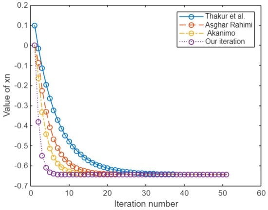
The iterative scheme converges to (34) for the operator defined in Equation (35) which is shown in Table 2 and Figure 2.

Table 2. Comparing iteration convergence.

No. of Iterations	Akanimo	Thakur	Asghar Rahimi	New Iteration
1	0.1	0.1	0.1	0.1
2	−0.0644720187	−0.0869402962	−0.1630096033	−0.3803139327
3	−0.1922289988	−0.2264595551	−0.3322517610	−0.5494920044
4	−0.2915201418	−0.3306827011	−0.4414827416	−0.6100326607
5	−0.3687681179	−0.4086549542	−0.5122262545	−0.6318737760
6	−0.4289375510	−0.4670790018	−0.5581749961	−0.6397788231
7	−0.4758578291	−0.5109175395	−0.5880826744	−0.6426433848
8	−0.5124838838	−0.5438511695	−0.6075783795	−0.6436818788
9	−0.5410994344	−0.5686166193	−0.6202998349	−0.6440584262
10	−0.5634729424	−0.5872541993	−0.6286065855	−0.6441949665
⋮	⋮	⋮	⋮	⋮
48	−0.6442665057	−0.6442716845	−0.6442726463	−0.6442726473
49	−0.6442678310	−0.6442719208	−0.6442726467	−0.6442726473
50	−0.6442688702	−0.6442720992	−0.6442726469	−0.6442726473

Figure 2. Comparison of iteration processes convergence [22].

Remark 3.

It is visible that after 7 iterations, new iteration (9) converges to solution of problem (33) up to 2 decimals faster than the iterative techniques [22,23,24], and after 50 iterations, ita convergence rate is faster than iterative techniques [22,23,24], as shown in Table 2 and Figure 2.

5.2. Delay Differential Equations

A delay differential equation (DDE) is a class of differential equations that includes terms dependent on past values of the solution. It takes the following form:

$${\displaystyle \frac{dy\left(t\right)}{dt}}=f(t,y\left(t\right),y(t-\tau ))$$

where $y\left(t\right)$ is the unknown function of time t, $\tau$ is the delay parameter and f is a function that describes how the rate of change of y depends on both the current state $y\left(t\right)$ and the state at an earlier time $y(t-\tau )$. This inclusion of past states allows DDEs to model systems where historical information impacts future dynamics, such as in biological, engineering or economic processes.

In this subsection, we use novel iterative scheme (9) to find the solution.

Consider $C\left(\right[u,v\left]\right)$, where the Banach space [33] of all continuous functions on closed interval $[u,v]$ has the Chebyshev norm defined as follows:

$${\left|\right|x-z\left|\right|}_{\infty }=\underset{r\in [u,v]}{sup}|x\left(r\right)-z\left(r\right)|.$$

We consider the following delay differential equation:

$$\begin{array}{c}\hfill x^{\prime }\left(r\right)=\psi (r,x\left(r\right),x(r-\gamma )),r\in [r_0,v]\end{array}$$

(36)

with initial condition

$$\begin{array}{c}\hfill x\left(r\right)=\zeta \left(r\right),r\in [r_0-\gamma ,r_0]\end{array}$$

(37)

A function $x\in C([r_0-\gamma ,v],\mathbb{R}) \cap C^1([r_0,v],\mathbb{R})$ that satisfies (36) and (37) is the solution of (36).

We further suppose that the following conditions are satisfied:

• $r_0,v\in \mathbb{R},\gamma >0$,
• $\psi \in C([r_0,v]\times {\mathbb{R}}^2,\mathbb{R}),$
• $\zeta \in C([r_0-\gamma ,v],\mathbb{R}),$
• There exists $Q_{\psi }>0$ such that:

  $$\begin{array}{c}\hfill |\psi (r,s_1,s_2)-\psi (r,t_1,t_2)|\le Q_{\psi }\sum _{i=1}^2|s_i-t_i|,s_i,t_i\in \mathbb{R},r\in [r_o,v]\end{array}$$

  (38)
• $2Q_{\psi }(v-r_0)<1$.

Using (36) and (37), we construct the integral equation as follows:

$$\begin{array}{c}\hfill x\left(r\right)=\left\{\begin{array}{c}\zeta \left(r\right),r\in [r_0-\gamma ,v]\hfill \\ \zeta \left(r_0\right)+{\int }_{r_0}^r\psi (t,x\left(t\right),x(t-\gamma ))dt,r\in [r_0,v].\hfill \end{array}\right.\end{array}$$

(39)

We present the following result as a generalization of the result of Coman et al. [34].

Theorem 4.

Suppose conditions $\left(1\right)$ to $\left(5\right)$ are satisfied. Then, (36) and (37) have the unique solution $x^{*}\in C([r_0-\gamma ,v],\mathbb{R}) \cap C^1([r_0,v],\mathbb{R})$, and the iterative scheme (9) converges to $x^{*}$ and

$$\begin{array}{c}\hfill x^{*}=\underset{n\to \infty }{lim}{T}^n\left(x\right)\end{array}$$

(40)

Proof. 

Let $x_n$ be the iterative scheme defined by (9) for an operator T given in (39).

Let $x^{*}\in F\left(T\right)$. We show that $x_n\to x^{*}$ as $n\to \infty$ for each $r\in [r_0-\gamma ,r_0].$

Now, for each $r\in [r_0,v]$, we have

$$\begin{array}{ccc}\hfill \parallel z_n-x^{*}{\parallel }_{\infty }& =& \parallel T((1-O_n)x_n+O_{n}T{x}_n)-x^{*}{\parallel }_{\infty }\hfill \\ & \le & \underset{r\in [r_0,v]}{sup}\left|T\left(((1-O_n)x_n+O_{n}T{x}_n)\right)\left(t\right)-T{x}^{*}\left(t\right)\right|\hfill \\ & \le & \underset{r\in [r_0,v]}{sup}\left|\zeta \left(r_0\right)+{\int }_{r_0}^r\psi (s,((1-O_n)x_n+O_{n}T{x}_n)\left(s\right),\right.\hfill \\ & & ((1-O_n)x_n+O_{n}T{x}_n\left)(s-\gamma )\right)ds\hfill \\ & & \left.-\left(\zeta \left(r_0\right)+{\int }_{r_0}^r\psi (s,x^{*}\left(s\right),x^{*}(s-\gamma ))ds\right)\right|\hfill \\ & \le & {\int }_{r_0}^r\left|\psi (s,((1-O_n)x_n+O_{n}T{x}_n)\left(s\right),\right.\hfill \\ & & \left.((1-O_n)x_n+O_{n}T{x}_n\left)(s-\gamma )\right)ds-\psi (s,x^{*}\left(s\right),x^{*}(s-\gamma ))ds)\right|\hfill \end{array}$$

(41)

$$\begin{array}{ccc} & \le & \underset{r\in [r_0,v]}{sup}{\int }_{r_0}^r{L}_{\psi }\left(\left|((1-O_n)x_n+O_{n}T{x}_n)\left(s\right)-x^{*}\left(s\right)\right|\right.\hfill \\ & & \left.+\left|((1-O_n)x_n+O_{n}T{x}_n)(s-\gamma )-x^{*}(s-\gamma )\right|\right)ds\hfill \\ & \le & {\int }_{r_0}^r{L}_{\psi }\left(\underset{r\in [r_0,v]}{sup}\left|((1-O_n)x_n+O_{n}T{x}_n)\left(s\right)-x^{*}\left(s\right)\right|\right.\hfill \\ & & \left.+\underset{r\in [r_0,v]}{sup}\left|((1-O_n)x_n+O_{n}T{x}_n)(s-\gamma )-x^{*}(s-\gamma )\right|\right)ds\hfill \\ & \le & {\int }_{r_0}^r{L}_{\psi }\left(\parallel ((1-O_n)x_n+O_{n}T{x}_n)\left(s\right)-x^{*}\left(s\right){\parallel }_{\infty }\right.\hfill \\ & & \left.+\parallel ((1-O_n)x_n+O_{n}T{x}_n)\left(s\right)-x^{*}\left(s\right){\parallel }_{\infty }\right)ds\hfill \\ & \le & 2L_{\psi }(v-r_0){\parallel ((1-O_n)x_n+O_{n}T{x}_n)\left(s\right)-x^{*}\left(s\right)\parallel }_{\infty }.\hfill \end{array}$$

(42)

$$\begin{array}{ccc}\hfill \parallel ((1-O_n)x_n+O_{n}T{x}_n)-x^{*}{\parallel }_{\infty }& =& \parallel ((1-O_n)x_n+O_{n}T{x}_n)-x^{*}{\parallel }_{\infty }\hfill \\ & \le & (1-O_n)\parallel x_n-x^{*}{\parallel }_{\infty }+O_n{\parallel T{x}_n-T{x}^{*}\parallel }_{\infty }\hfill \\ & \le & (1-O_n){\parallel x_n-x^{*}\parallel }_{\infty }+O_n\underset{r\in [r_0,v]}{sup}\hfill \\ & & \left(\left|{\int }_{r_0}^r\psi (s,(x_n\left(s\right),x_n(s-\gamma )ds-{\int }_{r_0}^r\psi (s,x^{*}\left(s\right),x^{*}(s-\gamma ))ds\right|\right)\hfill \\ & \le & (1-O_n){\parallel x_n-x^{*}\parallel }_{\infty }\hfill \\ & +& O_n{\int }_{r_0}^r{L}_{\psi }\left|\right|x_n\left(s\right)-x^{*}\left(s\right){\left|\right|}_{\infty }+\left|\right|x_n\left(s\right)-x^{*}\left(s\right){\left|\right|}_{\infty }ds\hfill \\ & \le & (1-O_n)\parallel x_n-x^{*}{\parallel }_{\infty }+O_{n}2L_{\psi }(v-r_0)\left|\right|x_n-x^{*}{\left|\right|}_{\infty }\hfill \\ & \le & [1-O_n(1-2L_{\psi }(v-r_0))]\left|\right|x_n-x^{*}{\left|\right|}_{\infty }\hfill \end{array}$$

(43)

Moreover,

$$\begin{array}{ccc}\hfill \parallel y_n-x^{*}{\parallel }_{\infty }& =& \parallel T((1-N_n)x_n+N_{n}T{z}_n)-x^{*}{\parallel }_{\infty }\hfill \\ & \le & \underset{r\in [r_0,v]}{sup}\left|T\left(((1-N_n)x_n+N_{n}T{z}_n)\right)\left(t\right)-T{x}^{*}\left(t\right)\right|\hfill \\ & \le & \underset{r\in [r_0,v]}{sup}\hfill \\ & & \left|\zeta \left(r_0\right)+{\int }_{r_0}^r\psi (s,((1-N_n)x_n+N_{n}T{z}_n)\left(s\right),\right.\hfill \\ & & \left.((1-N_n)x_n+N_{n}T{z}_n\left)(s-\gamma )\right)ds-\left(\zeta \left(r_0\right)+{\int }_{r_0}^r\psi (s,x^{*}\left(s\right),x^{*}(s-\gamma ))ds\right)\right|\hfill \\ & \le & {\int }_{r_0}^r\left|\psi (s,((1-N_n)x_n+N_{n}T{z}_n)\left(s\right),\right.\hfill \end{array}$$

(44)

$$\begin{array}{ccc} & & \left.((1-N_n)x_n+N_{n}T{z}_n\left)(s-\gamma )\right)ds-\psi (s,x^{*}\left(s\right),x^{*}(s-\gamma ))ds)\right|\hfill \\ & \le & \underset{r\in [r_0,v]}{sup}{\int }_{r_0}^r{L}_{\psi }\left(\left|((1-N_n)x_n+N_{n}T{z}_n)\left(s\right)-x^{*}\left(s\right)\right|\right.\hfill \\ & & \left.+\left|((1-N_n)x_n+N_{n}T{z}_n)(s-\gamma )-x^{*}(s-\gamma )\right|\right)ds\hfill \\ & \le & {\int }_{r_0}^r{L}_{\psi }\left(\underset{r\in [r_0,v]}{sup}\left|((1-N_n)x_n+N_{n}T{z}_n)\left(s\right)-x^{*}\left(s\right)\right|\right.\hfill \\ & & \left.+\underset{r\in [r_0,v]}{sup}\left|((1-N_n)x_n+N_{n}T{z}_n)(s-\gamma )-x^{*}(s-\gamma )\right|\right)ds\hfill \\ & \le & {\int }_{r_0}^r{L}_{\psi }\left(\parallel ((1-N_n)x_n+N_{n}T{z}_n)\left(s\right)-x^{*}\left(s\right){\parallel }_{\infty }\right.\hfill \\ & & \left.+\parallel ((1-N_n)x_n+N_{n}T{z}_n)\left(s\right)-x^{*}\left(s\right){\parallel }_{\infty }\right)ds\hfill \\ & \le & 2L_{\psi }(v-r_0){\parallel ((1-N_n)x_n+N_{n}T{z}_n)\left(s\right)-x^{*}\left(s\right)\parallel }_{\infty }.\hfill \end{array}$$

(45)

$$\begin{array}{ccc}\hfill \parallel ((1-N_n)x_n+N_{n}T{z}_n)-x^{*}{\parallel }_{\infty }& =& \parallel ((1-N_n)x_n+N_{n}T{z}_n)-x^{*}{\parallel }_{\infty }\hfill \\ & \le & (1-N_n)\parallel x_n-x^{*}{\parallel }_{\infty }+N_n{\parallel T{z}_n-T{x}^{*}\parallel }_{\infty }\hfill \\ & \le & (1-N_n){\parallel x_n-x^{*}\parallel }_{\infty }+N_n\underset{r\in [r_0,v]}{sup}\hfill \\ & & \left(\left|{\int }_{r_0}^r\psi (s,(z_n\left(s\right),z_n(s-\gamma )ds-{\int }_{r_0}^r\psi (s,x^{*}\left(s\right),x^{*}(s-\gamma ))ds\right|\right)\hfill \\ & \le & (1-N_n){\parallel x_n-x^{*}\parallel }_{\infty }\hfill \\ & +& N_n{\int }_{r_0}^r{L}_{\psi }\left|\right|z_n\left(s\right)-x^{*}\left(s\right){\left|\right|}_{\infty }+\left|\right|z_n\left(s\right)-x^{*}\left(s\right){\left|\right|}_{\infty }ds\hfill \\ & \le & (1-N_n)\parallel x_n-x^{*}{\parallel }_{\infty }+N_{n}2L_{\psi }(v-r_0)\left|\right|z_n-x^{*}{\left|\right|}_{\infty }\hfill \\ & \le & (1-N_n){\parallel x_n-x^{*}\parallel }_{\infty }+N_{n}2L_{\psi }(v-r_0)\hfill \\ & & [1-O_n(1-2L_{\psi }(v-r_0))]\left|\right|x_n-x^{*}{\left|\right|}_{\infty }\hfill \\ & \le & [1-N_n(1-2L_{\psi }(v-r_0))][1-O_n(1-2L_{\psi }(v-r_0))]\hfill \\ & & \left|\right|x_n-x^{*}{\left|\right|}_{\infty }\hfill \end{array}$$

(46)

and

$$\begin{array}{ccc}\hfill \parallel p_n-x^{*}{\parallel }_{\infty }& =& \parallel T\left((1-M_n)T{z}_n+M_{n}T{y}_n\right)-x^{*}{\parallel }_{\infty }\hfill \\ & \le & \underset{r\in [r_0,v]}{sup}\left|T\left(\left(1-M_n\right)T{z}_n+M_{n}T{y}_n\right)\left(t\right)-T{x}^{*}\left(t\right)\right|\hfill \\ & \le & \underset{r\in [r_0,v]}{sup}\left|\zeta \left(r_0\right)+{\int }_{r_0}^r\psi \left(s,\left(1-M_n\right)T{z}_n\left(s\right)+M_{n}T{y}_n\left(s\right),\right.\right.\hfill \\ & & \left.\left(1-M_n\right)T{z}_n(s-\gamma )+M_{n}T{y}_n(s-\gamma )\right)ds\hfill \\ & & \left.-\left(\zeta \left(r_0\right)+{\int }_{r_0}^r\psi \left(s,x^{*}\left(s\right),x^{*}(s-\gamma )\right)ds\right)\right|\hfill \end{array}$$

(47)

$$\begin{array}{ccc} & \le & {\int }_{r_0}^r\left|\psi \left(s,\left(1-M_n\right)T{z}_n\left(s\right)+M_{n}T{y}_n\left(s\right),\right.\right.\hfill \\ & & \left.\left.\left(1-M_n\right)T{z}_n(s-\gamma )+M_{n}T{y}_n(s-\gamma )\right)-\psi \left(s,x^{*}\left(s\right),x^{*}(s-\gamma )\right)\right|ds\hfill \\ & \le & {\int }_{r_0}^r{L}_{\psi }\left(\underset{r\in [r_0,v]}{sup}\left|\left(1-M_n\right)T{z}_n\left(s\right)+M_{n}T{y}_n\left(s\right)-x^{*}\left(s\right)\right|\right.\hfill \\ & & \left.+\underset{r\in [r_0,v]}{sup}\left|\left(1-M_n\right)T{z}_n(s-\gamma )+M_{n}T{y}_n(s-\gamma )-x^{*}(s-\gamma )\right|\right)ds\hfill \\ & \le & {\int }_{r_0}^r{L}_{\psi }\left(\parallel \left(1-M_n\right)T{z}_n\left(s\right)+M_{n}T{y}_n\left(s\right)-x^{*}{\left(s\right)\parallel }_{\infty }\right.\hfill \\ & & \left.+\parallel \left(1-M_n\right)T{z}_n(s-\gamma )+M_{n}T{y}_n(s-\gamma )-x^{*}{(s-\gamma )\parallel }_{\infty }\right)ds\hfill \\ & \le & 2L_{\psi }(v-r_0){\parallel (1-M_n)T{z}_n+M_{n}T{y}_n-x^{*}\left(s\right)\parallel }_{\infty }.\hfill \end{array}$$

(48)

$$\begin{array}{ccc}\hfill \parallel ((1-M_n)T{z}_n+M_{n}T{y}_n)-x^{*}{\parallel }_{\infty }& =& \parallel ((1-M_n)T{z}_n+M_{n}T{y}_n)-T{x}^{*}{\parallel }_{\infty }\hfill \\ & \le & (1-M_n)\parallel T{z}_n-T{x}^{*}{\parallel }_{\infty }+M_n{\parallel T{y}_n-T{x}^{*}\parallel }_{\infty }\hfill \\ & \le & (1-M_n)\underset{r\in [r_0,v]}{sup}\hfill \\ & & \left(\left|{\int }_{r_0}^r\psi (s,(z_n\left(s\right),z_n(s-\gamma )ds-{\int }_{r_0}^r\psi (s,x^{*}\left(s\right),x^{*}(s-\gamma ))ds\right|\right)\hfill \\ & +& M_n\underset{r\in [r_0,v]}{sup}\hfill \\ & & \left(\left|{\int }_{r_0}^r\psi (s,(y_n\left(s\right),y_n(s-\gamma )ds-{\int }_{r_0}^r\psi (s,x^{*}\left(s\right),x^{*}(s-\gamma ))ds\right|\right)\hfill \\ & \le & (1-M_n){\int }_{r_0}^r{L}_{\psi }\left|\right|z_n\left(s\right)-x^{*}\left(s\right){\left|\right|}_{\infty }+\left|\right|z_n\left(s\right)-x^{*}\left(s\right){\left|\right|}_{\infty }ds\hfill \\ & +& M_n{\int }_{r_0}^r{L}_{\psi }\left|\right|y_n\left(s\right)-x^{*}\left(s\right){\left|\right|}_{\infty }+\left|\right|y_n\left(s\right)-x^{*}\left(s\right){\left|\right|}_{\infty }ds\hfill \\ & \le & (1-M_n)2L_{\psi }(v-r_0)\left|\right|z_n-x^{*}{\left|\right|}_{\infty }\hfill \\ & +& M_{n}2L_{\psi }(v-r_0)\left|\right|y_n-x^{*}{\left|\right|}_{\infty }\hfill \\ & \le & (1-M_n)2L_{\psi }(v-r_0)[1-O_n(1-2L_{\psi }(v-r_0))]+M_{n}2\hfill \\ & & L_{\psi }(v-r_0)[1-N_n(1-2L_{\psi }(v-r_0))]\hfill \\ & & [1-O_n(1-2L_{\psi }(v-r_0))]\left|\right|x_n-x^{*}{\left|\right|}_{\infty }\hfill \\ & =& 2L_{\psi }(v-r_0)\hfill \\ & & [1-(1-2L_{\psi }(v-r_0))\left(M_n{N}_n+O_n-M_n{N}_n{O}_n\right)]\hfill \\ & & \left|\right|x_n-x^{*}{\left|\right|}_{\infty }\hfill \end{array}$$

(49)

Finally,

$$\begin{array}{ccc}\hfill \parallel x_{n+1}-x^{*}{\parallel }_{\infty }& =& \parallel T\left(T{p}_n\right)-x^{*}{\parallel }_{\infty }\hfill \\ & \le & \underset{r\in [r_0,v]}{sup}\left|T\left(T{p}_n\right)\left(t\right)-T{x}^{*}\left(t\right)\right|\hfill \\ & \le & \underset{r\in [r_0,v]}{sup}\hfill \end{array}$$

(50)

$$\begin{array}{ccc} & & \left|\zeta \left(r_0\right)+{\int }_{r_0}^r\psi (s,T{p}_n\left(s\right),T{p}_n(s-\gamma ))ds-\left(\zeta \left(r_0\right)+{\int }_{r_0}^r\psi (s,x^{*}\left(s\right),x^{*}(s-\gamma ))ds\right)\right|\hfill \\ & \le & {\int }_{{r_0}^r}\left|\psi (s,T{p}_n\left(s\right),T{p}_n(s-\gamma ))ds-\psi (s,x^{*}\left(s\right),x^{*}(s-\gamma ))ds)\right|\hfill \\ & \le & \underset{r\in [r_0,v]}{sup}{\int }_{r_0}^r{L}_{\psi }(\left|T{p}_n\left(s\right)-x^{*}\left(s\right)\right|+\left|T{p}_n(s-\gamma )-x^{*}(s-\gamma )\right|)ds\hfill \\ & \le & {\int }_{r_0}^r{L}_{\psi }\left(\underset{r\in [r_0,v]}{sup}(\left|T{p}_n\left(s\right)-x^{*}\left(s\right)\right|+\underset{r\in [r_0,v]}{sup}\left|T{p}_n(s-\gamma )-x^{*}(s-\gamma )\right|)\right)ds\hfill \\ & \le & {\int }_{r_0}^r{L}_{\psi }\left(\right||T{p}_n\left(s\right)-x^{*}{\left(s\right)\left|\right|}_{\infty }+\left|\right|T{p}_n\left(s\right)-x^{*}{\left(s\right)\left|\right|}_{\infty })ds\hfill \\ & \le & 2L_{\psi }(v-r_0)\left|\right|T{p}_n-x^{*}{\left|\right|}_{\infty }.\hfill \end{array}$$

(51)

$$\begin{array}{ccc}\hfill \parallel T{p}_n-x^{*}{\parallel }_{\infty }& =& \parallel T\left(p_n\right)-x^{*}{\parallel }_{\infty }\hfill \\ & \le & \underset{r\in [r_0,v]}{sup}\left|T\left(p_n\right)\left(t\right)-T{x}^{*}\left(t\right)\right|\hfill \\ & \le & \underset{r\in [r_0,v]}{sup}\hfill \\ & & \left|\zeta \left(r_0\right)+{\int }_{r_0}^r\psi (s,p_n\left(s\right),p_n(s-\gamma ))ds-\left(\zeta \left(r_0\right)+{\int }_{r_0}^r\psi (s,x^{*}\left(s\right),x^{*}(s-\gamma ))ds\right)\right|\hfill \\ & \le & {\int }_{r_0}^r\left|\psi (s,p_n\left(s\right),p_n(s-\gamma ))ds-\psi (s,x^{*}\left(s\right),x^{*}(s-\gamma ))ds)\right|\hfill \\ & \le & \underset{r\in [r_0,v]}{sup}{\int }_{r_0}^r{L}_{\psi }(\left|p_n\left(s\right)-x^{*}\left(s\right)\right|+\left|p_n(s-\gamma )-x^{*}(s-\gamma )\right|)ds\hfill \\ & \le & {\int }_{r_0}^r{L}_{\psi }\left(\underset{r\in [r_0,v]}{sup}(\left|p_n\left(s\right)-x^{*}\left(s\right)\right|+\underset{r\in [r_0,v]}{sup}\left|p_n(s-\gamma )-x^{*}(s-\gamma )\right|)\right)ds\hfill \\ & \le & {\int }_{r_0}^r{L}_{\psi }\left(\right||p_n\left(s\right)-x^{*}{\left(s\right)\left|\right|}_{\infty }+\left|\right|p_n\left(s\right)-x^{*}{\left(s\right)\left|\right|}_{\infty })ds\hfill \\ & \le & 2L_{\psi }(v-r_0)\left|\right|p_n-x^{*}{\left|\right|}_{\infty }.\hfill \\ & =& 2{L_{\psi }(v-r_0)}^2\hfill \\ & & [1-(1-2L_{\psi }(v-r_0))\left(M_n{N}_n+O_n-M_n{N}_n{O}_n\right)]\hfill \\ & & \left|\right|x_n-x^{*}{\left|\right|}_{\infty }\hfill \end{array}$$

(52)

□

Remark 4.

By condition 5 and as $[1-(1-2L_{\psi }(v-r_0))(M_n{N}_n+O_n-M_n{N}_n{O}_n\left)\right]={\tau }_n<1$ and $\left|\right|x_n-x^{*}{\left|\right|}_{\infty }=r_n$, the conditions of Lemma 3 of [35] are satisfied. Hence, ${lim}_{n\to \infty }\left|\right|x_n-x^{*}{\left|\right|}_{\infty }=0$.

5.3. Implicit Neural Network

In this section, we present a modified implicit neural network which can be regard as an extension of the traditional feed-forward neural network.

Deep equilibrium (DEQ) models, an emerging class of implicit models that map inputs to fixed points in neural networks, are gaining popularity in the deep learning community. A deep equilibrium (DEQ) model deviates from classical depth by solving for the fixed point of a single nonlinear layer R. This structure allows for the decoupling of the layer’s internal structure (which regulates representational capacity) from how the fixed point is determined (which affects inference-time efficiency), which is typically carried out using classic techniques.

We aim to build the neural network given in Figure 3 that translates from a data space x to an inference space y. The implicit component of the network utilizes a latent space X, and data are translated through L maps of this latent space from x to X. We defined that T is a network operator that transforms $X\times x\to X$ by:

$$T(X,x)\stackrel{\Delta }{=}R(X,L(x\left)\right)$$

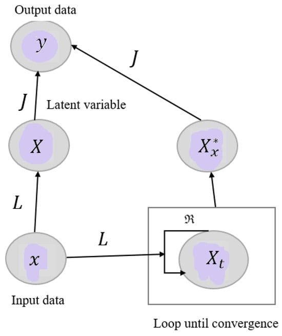
Figure 3. Feed-forward networks act by computing $J\circ L$. Implicit networks add a fixed point condition using R. When R is Garcia-Falset, repeatedly applying R to update a latent variable $x^k$ converges to a fixed point $x^{*}=R(x^{*};L\circ \left(x\right))$.

The objective is to find the unique fixed point $X_x^{*}$ of $T(.;x)$ given input data x. We will then use a final mapping $J:X\to y$ to transfer $X_x^{*}$ to the inference space y. Because of this, we can create an implicit network N by

$$N\left(x\right)\stackrel{\Delta }{=}J\left(X_x^{*}\right),\mathrm{where} T(X_x^{*}=X_x^{*},x)$$

Implicit models specify their outputs as solutions to nonlinear dynamical systems, as opposed to stacking a number of operators hierarchically. For instance, the outputs of DEQ models, which are the subject of this work, are defined as fixed points (i.e., equilibria) of a layer R and input x; that is, output

$$x^{*}=R(x^{*},x)$$

Theorem 5.

Let $\varnothing \ne C$ be a convex and closed subset of a UCBS and $\sigma :C\to C$ be a contraction mapping (activation function). Then, Equation (53) models well-posed and robust neural network provided that the weights {$M_t$}, {$N_t$}, {$O_t$},{$W_{(.)}$} and biases {$b_{(.)}$} are in [δ, 1 $-\delta$] for any $n\in \mathbb{N}$ and some $\delta \in (0,1)$.

$$\begin{array}{ccc}\hfill q_t& =& \sigma ((1-O_t)X+O_t\sigma \left(W_{1}X+W_2{P}_{t-1}+b_q\right))\hfill \\ \hfill r_t& =& \sigma ((1-N_t)X+N_t\sigma \left(W_3{q}_t+b_r\right))\hfill \\ \hfill z_t& =& \sigma ((1-M_t)\sigma \left(W_3{q}_t+b_r\right)+M_t\sigma \left(W_4{r}_t+b_z\right))\hfill \\ \hfill P_t& =& \sigma \left(W_5{z}_t+b_P\right)\hfill \\ \hfill X_t& =& \sigma \left(W_6{P}_t+b_y\right)\hfill \end{array}$$

(53)

Proof. 

Under the given conditions, Equation (53) models a well-posed system as the existence of unique fixed point for the contraction mapping $\sigma$ is guaranteed [17]. The robustness of system can be verified by Theorem 2 where the iterative scheme is proved to be T-stable, which shows that the smaller perturbation to the system does not effect the output. □

Example 4.

Training implicit neural network. Suppose we want to build a neural network that can predict an exam score based on the number of hours studied by assuming that whoever studies for $x\in [0,3]$ hours tends to achieve an exam score of $y\in [0,10]$, which can be defined by function $f\left(x\right)={\displaystyle \frac{10}{3}}x$. For this purpose, we train a network that takes an input of 3 (hours) and gives an output of 10 (score).

Key steps for solving iteration using implicit neural networks:

• FormulatetheProblem: Represent the task as a fixed-point equation.
• ChooseanIterativeSolver: Select an appropriate iterative method (4)–(7) to solve the implicit equation.
• Initialization: Define an initial guess for x and determine the conditions for convergence.
• BackpropagationthroughIterations: Implement the backpropagation process, considering the differentiation of the fixed-point iteration with respect to the parameters using implicit differentiation.
• ConvergenceandStabilityAnalysis: Analyze the convergence behavior and stability of the iterative process, ensuring that the method reliably finds a solution within the desired tolerance.

Given:

• Maximum input (max) = 3;
• Minimum input (min) = 0;
• Input value = 3.

Normalizing the input and output:

$$\mathit{normalized}\_\mathit{value}={\displaystyle \frac{\mathit{value}-min}{max-min}}$$

we get:

$$\mathit{normalized}\_\mathit{value}={\displaystyle \frac{3-0}{3-0}}={\displaystyle \frac{3}{3}}=1$$

By normalization, input 3 becomes 1, and similarly, output 10 also becomes 1. We start the Example by taking the following:

• Input $X=1$;
• Weights: $W_1=0.1,W_2=0.2,W_3=0.3,W_4=0.4,W_5=0.5,W_6=0.3$;
• Bias: $b_q=0.5,b_r=0.3,b_z=0.1,b_P=0.3,b_y=0.4$;
• $O=0.3,N=0.4,M=0.5$;
• Learning rate $\alpha =0.02$.

Novel Proposed Method:

We will compute $y_t$ using (53). For this, let us start by taking the activation function as $\sigma \left(x\right)={\displaystyle \frac{1}{1+exp(-x)}}$, which is a contraction on $(0,\infty )$.

At Time Step$t=1$:

Now applying our proposed iterative method, we obtain:

$$q_1=0.69$$

$$r_1=0.65$$

$$z_1=0.34$$

$$P_1=0.44$$

$$X_1=0.48$$

This will be output $y_t$ at time step $t=1$

Compute Loss:

The mean square error cost function is defined as follows:

$$C(W,b)=\sum _x\left|\right|{\displaystyle \frac{1}{2}}{(y\left(x\right)-y_t)}^2\left|\right|$$

where:

• x: input;
• $y_t$: output at time step t;
• W: weights collected in the network;
• b: biases;
• $∥v∥$: usual length of vector v.

Let us use the Mean Squared Error (MSE) $Loss$. The true output is $y=1.00;$

$$Loss={\displaystyle \frac{1}{2}}{(y-y_1)}^2$$

$$={\displaystyle \frac{1}{2}}{(1.00-0.48)}^2\approx 0.52.$$

Backpropagation:

Now, by using backpropagation, we will update weights and biases.

$${\displaystyle \frac{\partial Loss}{\partial y_1}}=-(1.00-0.48)=-0.52$$

Gradient Learning Algorithm:

We will update weights and biases using the gradient learning algorithm. This technique can be written as follows:

$$P_{n+1}=P_n-\alpha \nabla f\left(P_n\right)$$

Updating  $W_6$:

$${\displaystyle \frac{\partial Loss}{\partial W_6}}={\displaystyle \frac{\partial Loss}{\partial y_1}}{\displaystyle \frac{\partial y_1}{\partial \sigma }}{\displaystyle \frac{\partial \sigma }{\partial W_6}}=-0.52\times (1-ta{n}^2\left(0.48\right))\times P_1=-0.52\times 0.76\times 0.44=-0.18$$

$$Updated{W}_6=W_6\left(previous\right)-0.2\times {\displaystyle \frac{\partial Loss}{\partial W_6}}=0.33$$

Updating $b_y$:

$${\displaystyle \frac{\partial Loss}{\partial b_y}}={\displaystyle \frac{\partial Loss}{\partial y_1}}{\displaystyle \frac{\partial y_1}{\partial \sigma }}{\displaystyle \frac{\partial \sigma }{\partial b_y}}=-0.52\times (1-ta{n}^2\left(0.48\right))=-0.41$$

$$Updated{b}_y=b_y\left(previous\right)-0.2\times {\displaystyle \frac{\partial Loss}{\partial b_y}}=0.48$$

In a similar way, we will calculate other weights and biases as well.

Updated Weights and Biases:

Weights	Biases
$W_1=0.10$	$b_q=0.50$
$W_2=0.20$	$b_r=0.30$
$W_3=0.30$	$b_z=0.10$
$W_4=0.40$	$b_P=0.31$
$W_5=0.50$	$b_y=0.48$
$W_6=0.33$

At Time Step$t=2$:

We will calculate output $y_2$ by using updated weights and biases.

Using the same procedure, we calculated

$$y_2=0.55$$

Compute $Loss$:

Let us use the Mean Squared Error (MSE) $Loss$.

$$Loss\approx 0.45.$$

By repeating the same procedure:

At Time Step $t=6$:

After 6 iterations, our model is trained and we obtain the following loss:

$$Loss\approx 0.27.$$

Now, as our model is trained, we will check at $x=0.5$ and see what the output for this will be. Output y at normalized input is

$$y=0.50$$

We obtained the estimated output $y=5.0$ (score) for an input of $x=\left(1.5\right)$ hours.

It is proven in Section 2 that the rate of convergence of the iterative scheme (9) is higher than several others; therefore, the convergence rate of the trained network (53) is higher than many traditional networks like FNN, RNN, etc.

Since the proposed iterative method is faster in its convergence rate, therefore, the implicit neural network operating on its basis also has an improved convergence rate.

6. Conclusions

This research presents a novel iterative scheme that converges faster than Picard [17], Thakur et al. [22], Asghar Rahimi [23], Sintunavarat iteration [36], Jubair et al. [37], Okeke and Abbas [38], Agarwal et al. [39] and Akanimo [24]. The comparison of (9) with other iterative schemes through an Example 2 is also demonstrated. Finally, applications raised from various fields of science are given to show the applicability of our scheme. As a future work, it would be very interesting to see the applicability of this iterative scheme for solving nonlinear ODEs and PDEs after discretization. For similar work, see [40].

References

- Alagoz, O.; Birol, G.; Sezgin, G. Numerical reckoning fixed points for Barinde mappings via a faster iteration process. Facta Univ. Ser. Math. Inform. 2008, 33, 295–305. [Google Scholar]
- Ullah, K.; Ahmad, J.; Arshad, M.; Ma, Z. Approximating fixed points using a faster iterative method and application to split feasibility problems. Computation 2021, 9, 90. [Google Scholar] [CrossRef]
- Censor, Y.; Elfving, T. A multiprojection algorithm using Bregman projections in a product space. Numer. Algorithms 1994, 8, 221–239. [Google Scholar] [CrossRef]
- Byrne, C. A unified treatment of some iterative algorithms in signal processing and image reconstruction. Inverse Prob. 2004, 20, 103–120. [Google Scholar] [CrossRef]
- López, G.; Márquez, V.M.; Xu, H.K. Halpern iteration for Nonexpansive mappings. Contemp. Math. 2010, 513, 211–231. [Google Scholar]
- Kirk, W.A. A fixed point Theorem for mappings which do not increase distances. Amer. Math. Mon. 1965, 72, 1004–1006. [Google Scholar] [CrossRef]
- Browder, F.E. Nonexpansive nonlinear operators in a Banach space. Proc. Natl. Acad. Sci. USA 1965, 54, 1041–1044. [Google Scholar] [CrossRef]
- Göhde, D. Zum Prinzip der kontraktiven Abbildung. Math. Nachr. 1965, 30, 251–258. [Google Scholar] [CrossRef]
- Goebel, K. An elementary proof of the fixed-point Theorem of Browder and Kirk. Michigan Math. J. 1969, 16, 381–383. [Google Scholar] [CrossRef]
- Suzuki, T. Fixed point Theorems and convergence Theorems for some generalized nonexpansive mappings. J. Math. Anal. Appl. 2008, 340, 1088–1095. [Google Scholar] [CrossRef]
- Garcia-Falset, J.; Llorens-Fuster, E.; Suzuki, T. Fixed point theory for a class of generalized nonexpansive mappings. J. Math. Anal. Appl. 2011, 375, 185–195. [Google Scholar] [CrossRef]
- Bagherboum, M. Approximating fixed points of mappings satisfying condition (E) in Busemann space. Numer. Algorithms 2016, 71, 25–39. [Google Scholar] [CrossRef]
- Kitkuan, D.; Muangchoo, K.; Padcharoen, A.; Pakkaranang, N.; Kumam, P. A viscosity forward-backward splitting approximation method in Banach spaces and its application to convex optimization and image restoration problems. Comput. Math. Methods 2020, 2, e1098. [Google Scholar] [CrossRef]
- Kumam, W.; Pakkaranang, N.; Kumam, P.; Cholamjiak, P. Convergence analysis of modified Picard’s hybrid iterative algorithms for total asymptotically nonexpansive mappings in Hadamard spaces. Int. J. Comput. Math. 2020, 97, 157–188. [Google Scholar] [CrossRef]
- Sunthrayuth, P.; Pakkaranang, N.; Kumam, P.; Thounthong, P.; Cholamjiak, P. Convergence Theorems for generalized viscosity explicit methods for nonexpansive mappings in Banach spaces and some applications. Mathematics 2019, 7, 161. [Google Scholar] [CrossRef]
- Thounthong, P.; Pakkaranang, N.; Cho, Y.J.; Kumam, W.; Kumam, P. The numerical reckoning of modified proximal point methods for minimization problems in non-positive curvature metric spaces. J. Nonlinear Sci. Appl. 2020, 97, 245–262. [Google Scholar] [CrossRef]
- Picard, E. Mémoire sur la théorie des équations aux dérivées partielles et la méthode des approximations successives. J. Math. Pures Appl. 1890, 6, 145–210. [Google Scholar]
- Mann, W.R. Mean value methods in iteration. Proc. Amer. Math. Soc. 1953, 4, 506–510. [Google Scholar] [CrossRef]
- Ishikawa, S. Fixed points by a new iteration method. Proc. Amer. Math. Soc. 1974, 44, 147–150. [Google Scholar] [CrossRef]
- Noor, M.A. New approximation schemes for general variational inequalities. J. Math. Anal. Appl. 2000, 251, 217–229. [Google Scholar] [CrossRef]
- Abbas, M.; Nazir, T. A new faster iteration process applied to constrained minimization and feasibility problems. Mate. Vesnik 2014, 66, 223–234. [Google Scholar]
- Thakur, B.S.; Thakur, D.; Postolache, M. A new iteration scheme for approximating fixed points of nonexpansive mappings. Filomat 2015, 30, 2711–2720. [Google Scholar] [CrossRef]
- Rahimi, A.; Rezaei, A.; Daraby, B.; Ghasemi, M. A new faster iteration process to fixed points of generalized alpha-nonexpansive mappings in Banach spaces. Int. J. Nonlinear Anal. Appl. 2024, 15, 1–10. [Google Scholar]
- Okeke, G.A.; Udo, A.V.; Alqahtani, R.T.; Kaplan, M.; Ahmed, W.E. A novel iterative scheme for solving delay differential equations and third order boundary value problems via Green’s functions. AIMS Math. 2024, 9, 6468–6498. [Google Scholar] [CrossRef]
- Chen, T.Q.; Rubanova, Y.; Bettencourt, J.; Duvenaud, D. Neural ordinary differential equations. In Proceedings of the Advances in Neural Information Processing Systems 31 (NeurIPS 2018), Montréal, QC, Canada, 3–8 December 2018; Volume 31. [Google Scholar]
- Ghaoui, E.; Gu, F.; Travacca, B.; Askari, A.; Tsai, A. Implicit deep learning. Siam J. Math. Data Sci. 2021, 3, 930–950. [Google Scholar] [CrossRef]
- Bai, S.; Kolter, J.Z.; Koltun, V. Deep equilibrium models. arXiv 2019, arXiv:1909.01377. [Google Scholar]
- Kawaguchi, K. On the theory of implicit deep learning: Global convergence with implicit layers. arXiv 2021, arXiv:2102.07346. [Google Scholar]
- Jafarpour, S.; Davydov, A.; Proskurnikov, A.V.; Bullo, F. Robust implicit networks via non-Euclidean contractions. arXiv 2022, arXiv:2106.03194. [Google Scholar]
- Sahu, D.R. Applications of the S-iteration process to constrained minimization problems and split feasibility problems. Fixed Point Theory 2011, 12, 187–204. [Google Scholar]
- Gopi, R.; Pragadeeswarar, V.; De La Sen, M. Thakur’s Iterative Scheme for Approximating Common Fixed Points to a Pair of Relatively Nonexpansive Mappings. J. Math. 2022, 2022, 55377686. [Google Scholar] [CrossRef]
- Harder, A.M.; Hicks, T.L. A Stable Iteration Procedure for Nonexpansive Mappings. Math. Japon. 1988, 33, 687–692. [Google Scholar]
- Heammerlin, G.; Hoffmann, K.H. Numerical Mathematics; Springer Science and Business Media: Berlin/Heidelberg, Germany, 1991. [Google Scholar]
- Coman, G.; Rus, I.; Pavel, G.; Rus, I. Introduction in the Operational Equations Theory; Dacia: Cluj-Napoca, Romania, 1976. [Google Scholar]
- Weng, X. Fixed point iteration for local strictly pseudo-contractive mapping. Proc. Am. Math. Soc. 1991, 113, 727–731. [Google Scholar] [CrossRef]
- Sintunavarat, W.; Pitea, A. On a new iteration scheme for numerical reckoning fixed points of Berinde mappings with convergence analysis. J. Nonlinear Sci. Appl. 2016, 9, 2553–2562. [Google Scholar] [CrossRef]
- Ali, F.; Ali, J. Convergence, stability and data dependence of a new iterative algorithm with an application. Comput. Appl. Math. 2020, 39, 267. [Google Scholar] [CrossRef]
- Okeke, G.A.; Abbas, M. A solution of delay differential equations via Picard, Krasnoselskii hybrid iterative process. Arab. J. Math. 2017, 6, 21–29. [Google Scholar] [CrossRef]
- Agarwal, R.P.; O’Regan, D.; Sahu, D. Fixed Point Theory for Lipschitzian-Type Mappings with Applications; Springer: Berlin/Heidelberg, Germany, 2009. [Google Scholar]
- Wang, X. Fixed-Point Iterative Method with Eighth-Order Constructed by Undetermined Parameter Technique for Solving Nonlinear Systems. Symmetry 2021, 13, 863. [Google Scholar] [CrossRef]
Disclaimer/Publisher’s Note: The statements, opinions and data contained in all publications are solely those of the individual author(s) and contributor(s) and not of MDPI and/or the editor(s). MDPI and/or the editor(s) disclaim responsibility for any injury to people or property resulting from any ideas, methods, instructions or products referred to in the content. |
© 2025 by the authors. Licensee MDPI, Basel, Switzerland. This article is an open access article distributed under the terms and conditions of the Creative Commons Attribution (CC BY) license (https://creativecommons.org/licenses/by/4.0/).