On Fourier Series in the Context of Jacobi Matrices

Abstract

We investigate the properties of matrices that emerge from the application of Fourier series to Jacobi matrices. Specifically, we focus on functions defined by the coefficients of a Fourier series expressed in orthogonal polynomials. In the operational formulation of integro-differential problems, these infinite matrices play a fundamental role. We have derived precise calculation formulas for their elements, enabling exact computation of these operational matrices. Numerical results illustrate the effectiveness of our approach.

1. Introduction

This work presents a comprehensive investigation of matrices generated through the application of Fourier series to Jacobi matrices, with a particular focus on functions defined by Fourier series coefficients expressed in orthogonal polynomials. Precise formulas for computing the elements of these matrices are derived, which are crucial for the operational formulation of integro-differential problems. The fundamental properties of these matrices are highlighted, emphasizing their algebraic representation within functional operators. In numerical analysis, that representation gives rise to operational methods of which spectral methods are among a wide range of numerical tools to approximate solutions to integro-differential problems.

Let $\mathcal{D}:\mathbb{E}\mapsto \mathbb{F}$ be, at least approximately, a linear operator, with $\mathbb{E}$ and $\mathbb{F}$ being adequate function spaces, and let

$$\mathcal{D}y=f$$

(1)

be the problem to be solved, where $f\in \mathbb{F}$ is given and $y\in \mathbb{E}$ is the sought solution, at least approximately. Assuming that $\mathbb{P}$, the space of all real polynomials, is dense in $\mathbb{E}$, then y can be represented by a Fourier series:

$$y=\mathcal{P}\mathsf{a}\equiv \sum _{i=0}^{\infty }{a}_i{P}_i,$$

where $\mathcal{P}={\left[P_i\right]}_{i=0}^{\infty }\in \mathbb{P}$ is an orthogonal polynomial sequence (OPS) and $\mathsf{a}={[a_0,a_1,\dots ]}^T$ is the coefficients vector. The orthogonality of $\mathcal{P}$ ensures the existence of an inner product such that $⟨P_i,P_j⟩={\mu }_i{\delta }_{i,j}$, ${\delta }_{ij}$ is the Kronecker delta, and $a_i={\displaystyle \frac{1}{{\mu }_i}}⟨P_i,y⟩$ are the Fourier coefficients of y [1]. In addition, if $\mathbb{P}$ is also dense in $\mathbb{F}$, writing $f=\mathcal{P}\mathsf{f}$, then the problem of finding y in (1), given $\mathcal{D}$ and f, can be reduced to building $\mathsf{D}={\left[d_{i,j}\right]}_{i,j=0}^{\infty }$, the matrix operator such that

$$d_{i,j}={\displaystyle \frac{1}{{\mu }_i}}⟨P_i,\mathcal{D}{P}_j⟩$$

(2)

and solving the algebraic problem $\mathsf{D}\mathsf{a}=\mathsf{f}.$ Here, f corresponds, naturally, to the vector of Fourier coefficients of function f.

Building $\mathsf{D}$ is often a challenging task, involving numerically unstable and computationally heavy operations. Many mathematical problems can be modeled using derivatives and primitives, together with algebraic operations. For those cases, the matrix $\mathsf{D}$ can be built from three building blocks: the matrix $\mathsf{M}$, representing multiplication in $\mathcal{P}$; the matrix $\mathsf{N}$, representing differentiation; and the matrix $\mathsf{O}$, representing primitivation. Formally,

$$x\mathcal{P}=\mathcal{P}\mathsf{M},{\displaystyle \frac{d}{dx}}\mathcal{P}=\mathcal{P}\mathsf{N}\mathrm{and}\int \mathcal{P}=\mathcal{P}\mathsf{O}.$$

(3)

The linear integro-differential operator $\mathcal{D}$ can be cast in the form

$$\mathcal{D}=\sum _{k=-\eta }^{\nu }{f}_k{\displaystyle \frac{d^k}{d{x}^k}},$$

with $\nu ,\eta \ge 0$, where the negative indices represent primitives and $f_k$ the coefficients. Then, in matrix form,

$$\mathsf{D}=\sum _{k=-\eta }^{\nu }{f}_k\left(\mathsf{M}\right){\mathsf{N}}^k$$

where ${\mathsf{N}}^k$ corresponds to ${\mathsf{O}}^{-k}$ for negative powers. If $f_k={\sum }_{j=0}^{\infty }{f}_{k,j}{P}_j$ are functions given by its Fourier series, then

$$f_k\left(\mathsf{M}\right)=\sum _{j=0}^{\infty }{f}_{k,j}{P}_j\left(\mathsf{M}\right).$$

The paper is structured as follows: In Section 2 we derive properties of matrix polynomials $f_k\left(\mathsf{M}\right)$; in Section 3 we explore the functions of the matrix multiplication matrix; numerical results are provided to demonstrate the effectiveness of the proposed approach, showcasing the practical applicability of the derived formulas in Section 4; and we conclude in Section 5.

2. Polynomials of Jacobi Matrices

Using the well-known properties of orthogonal polynomials, we derive properties of matrix polynomials. In this context, we consider matrix polynomials as matrices transformed by polynomials with real scalar coefficients.

2.1. Orthogonal Polynomials

One characteristic property of orthogonal polynomials is the three-term recurrence relation. Let $\mathcal{P}={\left[P_i\right]}_{i=0}^{\infty }$ be an OPS satisfying

$$\left\{\begin{array}{c}{P}_{-1}=0,P_0=1\hfill \\ x{P}_j={\alpha }_j{P}_{j+1}+{\beta }_j{P}_j+{\gamma }_j{P}_{j-1},j=0,1,\dots ,\hfill \end{array}\right.$$

(4)

and let $\mathsf{A}={\left[a_{i,k}\right]}_{n\times n}$ be a square $n\times n$ real or complex matrix. We call ${\mathsf{P}}_j=P_j\left(\mathsf{A}\right),j=0,1,\dots$, the set of matrices defined by (4):

$${\mathsf{P}}_{j+1}={\displaystyle \frac{1}{{\alpha }_j}}(\mathsf{A}-{\beta }_j\mathsf{I}){\mathsf{P}}_j-{\displaystyle \frac{{\gamma }_j}{{\alpha }_j}}{\mathsf{P}}_{j-1},j=0,1,\dots ,$$

(5)

with ${\mathsf{P}}_{-1}=0$ and ${\mathsf{P}}_0=\mathsf{I}$ the null and the identity $n\times n$ matrices, respectively. Of course, since $\mathsf{A}$ and ${\mathsf{P}}_j$ are commutative matrices (${\mathsf{P}}_j$ is a linear combination of powers of $\mathsf{A}$), we can equivalently consider

$${\mathsf{P}}_{j+1}={\displaystyle \frac{1}{{\alpha }_j}}{\mathsf{P}}_j(\mathsf{A}-{\beta }_j\mathsf{I})-{\displaystyle \frac{{\gamma }_j}{{\alpha }_j}}{\mathsf{P}}_{j-1},j=0,1,\dots .$$

(6)

From (5), the rows of ${\mathsf{P}}_{j+1}$ can be evaluated by

$$e_i^T{\mathsf{P}}_{j+1}={\displaystyle \frac{1}{{\alpha }_j}}\sum _{k=0}^{n-1}{a}_{i,k}{e}_k^T{\mathsf{P}}_j-{\displaystyle \frac{{\beta }_j}{{\alpha }_j}}{e}_i^T{\mathsf{P}}_j-{\displaystyle \frac{{\gamma }_j}{{\alpha }_j}}{e}_i^T{\mathsf{P}}_{j-1},i=0,\dots ,n-1,$$

and from (6), the columns of ${\mathsf{P}}_{j+1}$ are given by

$${\mathsf{P}}_{j+1}{e}_k={\displaystyle \frac{1}{{\alpha }_j}}\sum _{i=0}^{n-1}{a}_{i,k}{\mathsf{P}}_j{e}_i-{\displaystyle \frac{{\beta }_j}{{\alpha }_j}}{\mathsf{P}}_j{e}_k-{\displaystyle \frac{{\gamma }_j}{{\alpha }_j}}{\mathsf{P}}_{j-1}{e}_k,k=0,\dots ,n-1.$$

For our purpose, we are interested in the case $\mathsf{A}=\mathsf{M}$, defined by (2) and (3), that is, $\mathsf{M}={\left[m_{i,j}\right]}_{i,j=0}^{\infty }$ with $m_{i,j}={\displaystyle \frac{1}{{\mu }_i}}⟨P_i,x{P}_j⟩$, and so, from (4),

$$\mathsf{M}=\left[\begin{array}{ccc}{\beta }_0& {\gamma }_1& \\ {\alpha }_0& {\beta }_1& {\gamma }_2& \\ & {\alpha }_1& {\beta }_2& & \\ & & {\alpha }_2& \\ & & & \cdots \end{array}\right]$$

(7)

is the Jacobi matrix associated with $\mathcal{P}$.

When considering the powers of such matrices, it is important to remember that they are infinite matrices. However, since each row and column of $\mathsf{M}$ contains only a finite number of non-zero elements, their products are well defined. Consequently, each power ${\mathsf{M}}^k$ with $k\in {\mathbb{N}}_0$ is well defined and has only a finite number of non-zero elements in each row and column.

In computational applications, to deal with $\mathsf{M}$ we have to truncate it to an ${\mathsf{M}}_{n\times n}$ square matrix for some $n\in \mathbb{N}$. One consequence of such a truncation operation is that elements outside the main block $(n-k)\times (n-k)$ of ${\mathsf{M}}^k$ can differ from the corresponding ones in ${\left({\mathsf{M}}_{n\times n}\right)}^k$. In practice, if we need to evaluate the main block $n\times n$ of ${\mathsf{M}}^k$ we must evaluate ${\left({\mathsf{M}}_{(n+k)\times (n+k)}\right)}^k$ and truncate the resulting square block.

In this work, we aim to evaluate $P_j\left(\mathsf{M}\right)$, where $P_j$ is the polynomials defined by (4) and $\mathsf{M}$ is its infinite Jacobi matrix defined by (7). As just explained, rather than performing matrix multiplications, we operate with the finite number of non-zero elements in each row and column of these matrices.

2.2. Linearization Coefficients

From now on, ${\mathsf{P}}_j=P_j\left(\mathsf{M}\right),j=0,1,\dots$ are the set of matrices defined by (5), with $\mathsf{A}=\mathsf{M}$ defined by (7). In that case, ${\mathsf{P}}_j$ are matrices of linearization coefficients, in the sense of:

Proposition 1. 

If $\mathcal{P}={\left[P_j\right]}_{j=0}^{\infty }$ is an OPS, $\mathsf{M}$ is its associated Jacobi matrix and ${\mathsf{P}}_j=P_j\left(\mathsf{M}\right),j=0,1,\dots$, then

$${\mathsf{P}}_j={\left[p_{jik}\right]}_{i,k=0}^{\infty },p_{jik}={\displaystyle \frac{1}{{\mu }_i}}⟨P_i,P_j{P}_k⟩.$$

Proof. 

Since, formally,

$$x\mathcal{P}=\mathcal{P}\mathsf{M},m_{ik}={\displaystyle \frac{1}{{\mu }_i}}⟨P_i,x{P}_k⟩,$$

then $x^j\mathcal{P}=\mathcal{P}{\mathsf{M}}^j,j=0,1,\dots$, and by linearity

$$P_j\left(x\right)\mathcal{P}=\mathcal{P}{P}_j\left(\mathsf{M}\right),p_{jik}={\displaystyle \frac{1}{{\mu }_i}}⟨P_i,P_j{P}_k⟩.$$

□

In the context of orthogonal polynomial theory, those values $p_{jik}$ are called linearization coefficients [2,3,4] because they solve the linearization problem

$$P_j{P}_k=\sum _{i=|j-k|}^{j+k}{p}_{jik}{P}_i.$$

(8)

It has been proven [2,3] that when $\mathcal{P}$ is a classical OPS the coefficients satisfy a second-order recurrence relation in the indices k. Furthermore, conditions have been established to ensure that ${\mathsf{P}}_j$ has only non-negative entries [4].

In search of specific cases, some authors have derived explicit formulas for these coefficients. Notable examples include the Legendre polynomials [5,6], the Hermite polynomials [7], and the Jacobi polynomials [8]. However, the formulas in some of these cases involve hypergeometric functions, which are not practical for numerical purposes. The linearization coefficients of the Chebyshev polynomials are particularly noteworthy due to their simplicity. Using the standard notation for the first, second, third, and fourth order of Chebyshev polynomials, we have found the following results [9,10] for $j=1,2,\dots$,

$$\begin{array}{ccc}\hfill {\displaystyle T_j{T}_k=\frac{1}{2}\left(T_{j+k}+T_{|j-k|}\right),}& & U_j{U}_k={\displaystyle \frac{1}{2}}\sum _{i=|j-k|}^{j+k}(1+{(-1)}^{j+k-i})U_i,\hfill \\ \hfill {\displaystyle V_j{V}_k=\sum _{i=|j-k|}^{j+k}{(-1)}^{j+k+i}{V}_i,}& & W_j{W}_k=\sum _{i=|j-k|}^{j+k}{W}_i,\hfill \end{array}$$

(9)

and, in the four cases, $P_0{P}_k=P_k$. In Figure 1, we can see the sparse structure of ${\mathsf{P}}_{15}$ matrices for those cases.

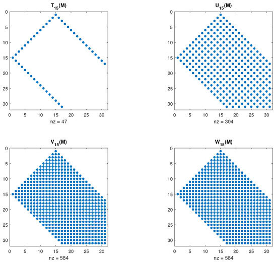
Figure 1. Sparse structure of ${\mathsf{P}}_{15}$, truncated to their $31\times 31$ main block, for T, U, V, and W, the first-, second-, third-, and fourth-kind Chebyshev polynomials, respectively.

This band structure, characterized by zeros outside the $\pm j$ diagonals and within the triangular block, $i=0,\dots ,|j-k|-1$, of matrices ${\mathsf{P}}_j$, is not exclusive to Chebyshev polynomials. In fact, it is a consequence of the general Formula (8), inherited from the three-term recurrence relation (4).

Proposition 2. 

If $\mathcal{P}={\left[P_j\right]}_{j=0}^{\infty }$ is an OPS satisfying (8), $\mathsf{M}$ is its associated Jacobi matrix and ${\mathsf{P}}_j=P_j\left(\mathsf{M}\right),j=0,1,\dots$, then

$${\mathsf{P}}_j={\left[p_{jik}\right]}_{i,k=0}^{\infty },\mathit{with}{p}_{jik}=\left\{\begin{array}{cc}1,\hfill & k=0\hfill \\ 0,\hfill & i>j+k\hfill \\ 0,\hfill & i<|j-k|\hfill \end{array}\right..$$

Proof. 

Considering $k=0$ in Equation (8) results in $P_j{P}_0=p_{jj0}{P}_j$, and since $P_0=1$ we obtain $p_{jj0}=0$. The proof ends considering that, for any $k>0$, Equation (8) is equivalent to

$$P_j{P}_k=\sum _{i=0}^{\infty }{p}_{jik}{P}_i,$$

for $i>j+k$ and for $i<|j-k|$. □

One immediate consequence of those triangular null blocks is that they include square main blocks inside.

Corollary 1. 

Let ${\mathsf{P}}_j=P_j\left(\mathsf{M}\right)$, defined as in Proposition 2, and let ${\left({\mathsf{P}}_j\right)}_{n\times n}={\left[p_{jik}\right]}_{i,k=0}^n$ be a square main block. If $j>2n$, then ${\left({\mathsf{P}}_j\right)}_{n\times n}=0$ is a null matrix.

Proof. 

Proposition 2 implies that $p_{jik}=0$ for any pair $i,k$ such that $i+k<j$, and this is valid if $i,k\le n$ and $j>2n$. □

Three additional consequences of Proposition 1 are as follows:

$$\left\{\begin{array}{c}{p}_{kij}=p_{jik}\hfill \\ p_{ijk}={\displaystyle \frac{{\mu }_i}{{\mu }_j}}{p}_{jik}\hfill \\ p_{jki}={\displaystyle \frac{{\mu }_i}{{\mu }_k}}{p}_{jik}\hfill \end{array}\right.,i,j,k=0,1,\dots .$$

The first one, meaning that each column j of a matrix ${\mathsf{P}}_k$ equals the column k of ${\mathsf{P}}_j$,

$${\mathsf{P}}_k{e}_j={\mathsf{P}}_j{e}_k,k,j=0,1,\dots ,$$

is a general property. The other two, relating each row j of ${\mathsf{P}}_i$ with row i of ${\mathsf{P}}_j$,

$$e_j^T{\mathsf{P}}_i={\displaystyle \frac{{\mu }_i}{{\mu }_j}}{e}_i^T{\mathsf{P}}_j,i,j=0,1,\dots ,$$

and ${\mathsf{P}}_j$ with its transpose,

$$e_k^T{\mathsf{P}}_j{e}_i={\displaystyle \frac{{\mu }_i}{{\mu }_k}}{e}_i^T{\mathsf{P}}_j{e}_k,i,j,k=0,1,\dots ,$$

are both verified if the associated inner product satisfies the wide general property $⟨P_i,P_j{P}_k⟩=⟨P_j,P_i{P}_k⟩$.

Next, we study the more general properties of the matrices ${\mathsf{P}}_j$, associated with generic OPSs, not limited to the classical ones.

2.3. General Properties of ${\mathsf{P}}_j$ Matrices

First of all, we can verify that any re-normalization in the polynomial sequence leads to similar matrices.

Proposition 3. 

Let $\hat{\mathcal{P}}={\left[{\hat{P}}_j\right]}_{j=0}^{\infty }$ such that ${\hat{P}}_j={\lambda }_j{P}_j$, with ${\lambda }_0=1$ and ${\lambda }_j\ne 0,j=1,2,\dots$; and let $\mathsf{M}$ and $\hat{\mathsf{M}}$ be the Jacobi matrices associated with $\mathcal{P}$ and $\hat{\mathcal{P}}$, respectively. Then, ${\hat{\mathsf{P}}}_j={\hat{P}}_j\left(\hat{\mathsf{M}}\right)$ and ${\mathsf{P}}_j=P_j\left(\mathsf{M}\right)$ are related by

$${\hat{\mathsf{P}}}_j={\lambda }_j{\mathsf{D}}^{-1}{\mathsf{P}}_j\mathsf{D},$$

(10)

with $\mathsf{D}=diag\left({\left[{\lambda }_j\right]}_{j=0}^{\infty }\right)$.

Proof. 

From (4) we obtain that

$$\left\{\begin{array}{c}{\hat{P}}_{-1}=0,{\hat{P}}_0=1\hfill \\ x{\hat{P}}_j={\hat{\alpha }}_j{\hat{P}}_{j+1}+{\hat{\beta }}_j{\hat{P}}_j+{\hat{\gamma }}_j{\hat{P}}_{j-1},j=0,1,\dots ,\hfill \end{array}\right.$$

with

$${\hat{\alpha }}_j={\displaystyle \frac{{\lambda }_j}{{\lambda }_{j+1}}}{\alpha }_j,{\hat{\beta }}_j={\beta }_j,\mathrm{and}{\hat{\gamma }}_{j+1}={\displaystyle \frac{{\lambda }_{j+1}}{{\lambda }_j}}{\gamma }_{j+1},j=0,1,\dots .$$

So, $\hat{\mathsf{M}}={\mathsf{D}}^{-1}\mathsf{M}\mathsf{D}$. Furthermore, ${\hat{\mathsf{P}}}_{-1}={\mathsf{P}}_{-1}=0,{\hat{\mathsf{P}}}_0={\mathsf{P}}_0=\mathsf{I}$, both satisfying (10), and

$$\begin{array}{ccc}\hfill {\hat{\mathsf{P}}}_{j+1}& =& {\displaystyle \frac{1}{{\hat{\alpha }}_j}}\left(\hat{\mathsf{M}}-{\hat{\beta }}_j\mathsf{I}\right){\hat{\mathsf{P}}}_j-{\displaystyle \frac{{\hat{\gamma }}_j}{{\hat{\alpha }}_j}}{\hat{\mathsf{P}}}_{j-1}\hfill \\ & =& {\displaystyle \frac{{\lambda }_{j+1}}{{\lambda }_j{\alpha }_j}}{\mathsf{D}}^{-1}\left(\mathsf{M}-{\beta }_j\mathsf{I}\right)\mathsf{D}{\hat{\mathsf{P}}}_j-{\displaystyle \frac{{\lambda }_{j+1}{\gamma }_j}{{\lambda }_{j-1}{\alpha }_j}}{\hat{\mathsf{P}}}_{j-1}.\hfill \end{array}$$

Then, by the induction hypothesis,

$$\begin{array}{ccc}\hfill {\hat{\mathsf{P}}}_{j+1}& =& {\lambda }_{j+1}{\mathsf{D}}^{-1}\left[{\displaystyle \frac{1}{{\alpha }_j}}\left(\mathsf{M}-{\beta }_j\mathsf{I}\right){\mathsf{P}}_j-{\displaystyle \frac{{\gamma }_j}{{\alpha }_j}}{\mathsf{P}}_{j-1}\right]\mathsf{D}\hfill \\ & =& {\lambda }_{j+1}{\mathsf{D}}^{-1}{\mathsf{P}}_{j+1}\mathsf{D}.\hfill \end{array}$$

□

Proposition 3 can be utilized to establish a connection between matrices ${\mathsf{P}}_j$ associated with any generic OPS and matrices ${\hat{\mathsf{P}}}_j$ linked to their respective monic orthogonal polynomial sequences, or to the corresponding orthonormal polynomial sequences.

Corollary 2. 

Let $\mathcal{P}={\left[P_j\right]}_{j=0}^{\infty }$ be an OPS with leading coefficients $c_j={\displaystyle \frac{1}{{\mu }_j}}⟨P_j,x^j⟩$, and let $\hat{\mathcal{P}}={\left[{\hat{P}}_j\right]}_{j=0}^{\infty }$ be the monic OPS ${\hat{P}}_j={\displaystyle \frac{1}{c_j}}{P}_j$, then

$${\hat{\mathsf{P}}}_j={\displaystyle \frac{1}{c_j}}{\mathsf{D}}^{-1}{\mathsf{P}}_j\mathsf{D},$$

where $\mathsf{D}$ is the diagonal matrix $\mathsf{D}={\left[{\displaystyle \frac{1}{c_j}}{\delta }_{i,j}\right]}_{i,j=0}^{\infty }$.

Corollary 3. 

Let $\mathcal{P}={\left[P_j\right]}_{j=0}^{\infty }$ be an OPS with polynomial norms $\parallel P_j{\parallel }^2={\mu }_j=⟨P_j,P_j⟩$, and let $\hat{\mathcal{P}}={\left[{\hat{P}}_j\right]}_{j=0}^{\infty }$ be the orthonormal polynomial sequence ${\hat{P}}_j={\displaystyle \frac{1}{\sqrt{{\mu }_j}}}{P}_j$, then

$${\hat{\mathsf{P}}}_j={\displaystyle \frac{1}{\sqrt{{\mu }_j}}}{\mathsf{D}}^{-1}{\mathsf{P}}_j\mathsf{D},$$

with $\mathsf{D}={\left[{\displaystyle \frac{1}{\sqrt{{\mu }_j}}}{\delta }_{i,j}\right]}_{i,j=0}^{\infty }$.

As pointed out in [11], the Jacobi matrix $\mathsf{M}$ associated with any OPS is similar to the symmetric matrix $\mathsf{J}$ associated with the corresponding orthonormal sequence. Indeed, $\mathsf{J}={\mathsf{D}}^{-1}\mathsf{M}\mathsf{D}$ is the symmetric matrix

$$\mathsf{J}=\left[\begin{array}{ccc}{\beta }_0& {\rho }_0& \\ {\rho }_0& {\beta }_1& {\rho }_1& \\ & {\rho }_1& {\beta }_2& \\ & & {\rho }_2& \\ & & & \cdots \end{array}\right],{\rho }_i=\sqrt{{\displaystyle \frac{{\mu }_{i+1}}{{\mu }_i}}}{\alpha }_i,$$

(11)

associated with the orthonormal polynomials

$$\left\{\begin{array}{c}{\hat{P}}_{-1}=0,{\hat{P}}_0=1\hfill \\ x{\hat{P}}_j={\rho }_j{\hat{P}}_{j+1}+{\beta }_j{\hat{P}}_j+{\rho }_{j-1}{\hat{P}}_{j-1},j=0,1,\dots .\hfill \end{array}\right.$$

(12)

From (11) and (12), we obtain symmetric matrices.

Proposition 4. 

Let $\hat{\mathcal{P}}={\left[{\hat{P}}_j\right]}_{j=0}^{\infty }$ be an orthonormal OPS defined by (12) and let $\mathsf{J}$ be its associated Jacobi matrix, then ${\hat{\mathsf{P}}}_j={\hat{P}}_j\left(\mathsf{J}\right),j=0,1,\dots$ are symmetric matrices.

Proof. 

Since ${\hat{\mathsf{P}}}_0=0$ and ${\hat{\mathsf{P}}}_1=\mathsf{I}$ are both symmetric matrices, the proof results from

$${\hat{\mathsf{P}}}_{j+1}={\displaystyle \frac{1}{{\rho }_j}}\left(\mathsf{J}-{\beta }_j\mathsf{I}\right){\hat{\mathsf{P}}}_j-{\displaystyle \frac{{\rho }_{j-1}}{{\rho }_j}}{\hat{\mathsf{P}}}_{j-1}$$

by the induction hypothesis in j and by the symmetry of $\mathsf{J}$. □

Another general property of ${\mathsf{P}}_j$ matrices is invariance under the orthogonality support of $\mathcal{P}$, in the sense of the following proposition:

Proposition 5. 

Let $\mathcal{P}={\left[P_i\right]}_{i=0}^{\infty }$ be the OPS defined by (4) and ${\mathcal{P}}^{*}={\left[P_i^{*}\right]}_{i=0}^{\infty }$ be the OPS defined by

$$\left\{\begin{array}{c}{P}_{-1}^{*}=0,P_0^{*}=1\hfill \\ x{P}_j^{*}={\alpha }_j^{*}{P}_{j+1}^{*}+{\beta }_j^{*}{P}_j^{*}+{\gamma }_j^{*}{P}_{j-1}^{*},j=0,1,\dots ,\hfill \end{array}\right.$$

with ${\alpha }_j^{*}={\displaystyle \frac{{\alpha }_j}{\lambda }},{\beta }_j^{*}={\displaystyle \frac{{\beta }_j-\delta }{\lambda }}$, and ${\gamma }_j^{*}={\displaystyle \frac{{\gamma }_j}{\lambda }}$ for some $\lambda ,\delta \in \mathbb{R}$, $\lambda \ne 0$. If $\mathsf{M}$ and ${\mathsf{M}}^{*}$ are the Jacobi matrices associated with $\mathcal{P}$ and ${\mathcal{P}}^{*}$, respectively, then

$$P_j^{*}\left({\mathsf{M}}^{*}\right)=P_j\left(\mathsf{M}\right),j=0,1,\dots .$$

Proof. 

From ${\mathsf{M}}^{*}={\displaystyle \frac{1}{\lambda }}(\mathsf{M}-\delta \mathsf{I})$, we have

$$\begin{array}{ccc}\hfill {\mathsf{P}}_{j+1}^{*}& =& {\displaystyle \frac{1}{{\alpha }_j^{*}}}({\mathsf{M}}^{*}-{\beta }_j^{*}\mathsf{I}){\mathsf{P}}_j^{*}-{\displaystyle \frac{{\gamma }_j^{*}}{{\alpha }_j^{*}}}{\mathsf{P}}_{j-1}^{*}\hfill \\ & =& {\displaystyle \frac{\lambda }{{\alpha }_j}}({\displaystyle \frac{1}{\lambda }}(\mathsf{M}-\delta \mathsf{I})-{\displaystyle \frac{{\beta }_j-\delta }{\lambda }}\mathsf{I}){\mathsf{P}}_j^{*}-{\displaystyle \frac{{\gamma }_j}{{\alpha }_j}}{\mathsf{P}}_{j-1}^{*}\hfill \\ & =& {\displaystyle \frac{1}{{\alpha }_j}}(\mathsf{M}-{\beta }_j\mathsf{I}){\mathsf{P}}_j^{*}-{\displaystyle \frac{{\gamma }_j}{{\alpha }_j}}{\mathsf{P}}_{j-1}^{*},j=0,1,\dots ,\hfill \end{array}$$

and ${\mathsf{P}}_{j+1}^{*}={\mathsf{P}}_{j+1}$, since ${\mathsf{P}}_{-1}^{*}={\mathsf{P}}_{-1}$ and ${\mathsf{P}}_0^{*}={\mathsf{P}}_0$. □

If $[a,b],b>a$ is the domain of orthogonality of $\mathcal{P}$ and $[c,d],d>c$ is the domain of orthogonality of ${\mathcal{P}}^{*}$, then the conditions of Proposition 5 hold, with $\lambda ={\displaystyle \frac{d-c}{b-a}}$ and $\delta ={\displaystyle \frac{bc-ad}{b-a}}$, and we obtain ${\mathsf{P}}_j^{*}={\mathsf{P}}_j$ for all j.

2.4. Recurrence Relations

Returning to recursive Formulas (5) and (6), taking $\mathsf{A}=\mathsf{M}$, we obtain

$$\begin{array}{ccc}\hfill e_i^T{\mathsf{P}}_{j+1}& =& {\displaystyle \frac{{\alpha }_{i-1}}{{\alpha }_j}}{e}_{i-1}^T{\mathsf{P}}_j+{\displaystyle \frac{1}{{\alpha }_j}}({\beta }_i-{\beta }_j)e_i^T{\mathsf{P}}_j+{\displaystyle \frac{{\gamma }_{i+1}}{{\alpha }_j}}{e}_{i+1}^T{\mathsf{P}}_j-{\displaystyle \frac{{\gamma }_j}{{\alpha }_j}}{e}_i^T{\mathsf{P}}_{j-1},\hfill \\ \hfill {\mathsf{P}}_{j+1}{e}_k& =& {\displaystyle \frac{{\gamma }_k}{{\alpha }_j}}{\mathsf{P}}_j{e}_{k-1}+{\displaystyle \frac{1}{{\alpha }_j}}({\beta }_k-{\beta }_j){\mathsf{P}}_j{e}_k+{\displaystyle \frac{{\alpha }_k}{{\alpha }_j}}{\mathsf{P}}_j{e}_{k+1}-{\displaystyle \frac{{\gamma }_j}{{\alpha }_j}}{\mathsf{P}}_{j-1}{e}_k,\hfill \end{array}$$

(13)

recursive formulas relating the rows and columns of ${\mathsf{P}}_{j+1}$ with those of ${\mathsf{P}}_j$ and ${\mathsf{P}}_{j-1}$. From their element-wise versions, we obtain a recursivity in ${\mathsf{P}}_j$ elements,

$$p_{j,i,k+1}={\displaystyle \frac{1}{{\alpha }_k}}\left[{\alpha }_{i-1}{p}_{j,i-1,k}+({\beta }_i-{\beta }_k)p_{j,i,k}+{\gamma }_{i+1}{p}_{j,i+1,k}-{\gamma }_k{p}_{j,i,k-1}\right],$$

(14)

for $i,j,k=0,1,\dots$, where $p_{i,j,k}=0$ whenever at least one index is negative.

From (13) we can take values for a matrix sequence ${\mathsf{P}}_j,j=1,2,\dots$. Recurrence relations (14) are useful in case only a single matrix ${\mathsf{P}}_j$ is needed. For the latter case, we need the first two columns for the initial values.

Proposition 6. 

Let $\mathcal{P}={\left[P_i\right]}_{i=0}^{\infty }$ be an OPS and $\mathsf{M}$ its associated Jacobi matrix. If ${\mathsf{P}}_j=P_j\left(\mathsf{M}\right)$ and $p_{j,i,k}=e_i^T{\mathsf{P}}_j{e}_k$, then for $i,j=0,1,\dots$,

(a) 

$p_{j,i,0}={\delta }_{i,j};$

(b) 

$p_{j,i,1}=\left\{\begin{array}{cc}{\displaystyle \frac{{\gamma }_j}{{\alpha }_0}},\hfill & i=j-1\hfill \\ {\displaystyle \frac{1}{{\alpha }_0}}({\beta }_j-{\beta }_0),\hfill & i=j\hfill \\ {\displaystyle \frac{{\alpha }_j}{{\alpha }_0}},\hfill & i=j+1\hfill \\ 0\hfill & |j-i|>1\hfill \end{array}\right..$

Proof. 

The proof of (a) is immediate from Proposition 2. (b) results from (a) and (14). □

Keeping in mind that ${\mathsf{P}}_j$ is a band matrix, from (14) we obtain explicit formulas for the sub-diagonals j and $j-1$.

Proposition 7. 

Let $\mathcal{P}={\left[P_i\right]}_{i=0}^{\infty }$ be an OPS, $c_j={\displaystyle \frac{1}{{\mu }_j}}⟨P_j,x^j⟩$ and $c_j^{\prime }={\displaystyle \frac{1}{{\mu }_j}}⟨P_j,x^{j-1}⟩$ its leading coefficients, and ${\mathsf{P}}_j=P_j\left(\mathsf{M}\right)$, then for $j,k=0,1,\dots$,

(a) 

${\displaystyle p_{j,j+k,k}=\frac{c_j{c}_k}{c_{j+k}}}$;

(b) 

${\displaystyle p_{j,j+k-1,k}=\frac{c_j{c}_k}{c_{j+k-1}}\left(\frac{c_j^{\prime }}{c_j}+\frac{c_k^{\prime }}{c_k}-\frac{c_{j+k}^{\prime }}{c_{j+k}}\right)}$.

Proof. 

For the proof, we need the well-known relations [9]

$${\alpha }_j={\displaystyle \frac{c_j}{c_{j+1}}},{\beta }_j={\displaystyle \frac{c_j^{\prime }}{c_j}}-{\displaystyle \frac{c_{j+1}^{\prime }}{c_{j+1}}},$$

and, since $c_0=1,c_0^{\prime }=0$, we have

$$\prod _{r=0}^n{\alpha }_r={\displaystyle \frac{1}{c_{n+1}}},\sum _{r=0}^n{\beta }_r=-{\displaystyle \frac{c_{n+1}^{\prime }}{c_{n+1}}}.$$

From (14) and Proposition 2,

$$p_{j,j+k,k}={\displaystyle \frac{{\alpha }_{j+k-1}}{{\alpha }_{k-1}}}{p}_{j,j+k-1,k-1}.$$

This is a recurrence relation that, with the initial value $p_{j,j,0}=1$ given in Proposition 6, results in

$$p_{j,j+k,k}={\displaystyle \frac{{\prod }_{r=j}^{j+k-1}{\alpha }_r}{{\prod }_{r=0}^{k-1}{\alpha }_r}}={\displaystyle \frac{{\prod }_{r=0}^{j+k-1}{\alpha }_r}{{\prod }_{r=0}^{j-1}{\alpha }_r{\prod }_{r=0}^{k-1}{\alpha }_r}}.$$

So (a) is proved.

Again, from (14) and Proposition 2,

$$p_{j,j+k-1,k}={\displaystyle \frac{{\alpha }_{j+k-2}}{{\alpha }_{k-1}}}{p}_{j,j+k-2,k-1}+{\displaystyle \frac{1}{{\alpha }_{k-1}}}({\beta }_{j+k-1}-{\beta }_{k-1})p_{j,j+k-1,k-1}$$

or

$$p_{j,j+k-1,k}={\displaystyle \frac{c_k{c}_{j+k-2}}{c_{k-1}{c}_{j+k-1}}}{p}_{j,j+k-2,k-1}+{\displaystyle \frac{c_j{c}_k}{c_{j+k-1}}}({\beta }_{j+k-1}-{\beta }_{k-1}),$$

with initial value $p_{j,j,1}={\displaystyle \frac{1}{{\alpha }_0}}({\beta }_j-{\beta }_0)=c_1({\beta }_j-{\beta }_0)$, results in

$$p_{j,j+k-1,k}={\displaystyle \frac{c_j{c}_k}{c_{j+k-1}}}\left(\sum _{r=j}^{j+k-1}{\beta }_r-\sum _{r=0}^{k-1}{\beta }_r\right)={\displaystyle \frac{c_j{c}_k}{c_{j+k-1}}}\left(\sum _{r=0}^{j+k-1}{\beta }_r-\sum _{r=0}^{j-1}{\beta }_r-\sum _{r=0}^{k-1}{\beta }_r\right),$$

and in (b). □

Similar results can be obtained for the first two non-null ${\mathsf{P}}_j$ anti-diagonals.

Proposition 8. 

In the conditions of Proposition 7, for $j=0,1,\dots$,

(a) 

${\displaystyle p_{j,j-k,k}=\frac{{\mu }_j{c}_k{c}_{j-k}}{{\mu }_{j-k}{c}_j}}$, for $k=0,\dots ,j$;

(b) 

${\displaystyle p_{j,j-k+1,k}=\frac{{\mu }_j{c}_k{c}_{j-k+1}}{{\mu }_{j-k+1}{c}_j}\left(\frac{c_{j-k+1}^{\prime }}{c_{j-k+1}}+\frac{c_k^{\prime }}{c_k}-\frac{c_{j+1}^{\prime }}{c_{j+1}}\right)}$, for $k=1,\dots ,j$.

Proof. 

Since $p_{j,j-k-1,k-1},p_{j,j-k,k-1}$, and $p_{j,j-k,k-2}$ belong to the null triangular block of ${\mathsf{P}}_j$, from (14) we have, for $k=0,\dots ,j$,

$$p_{j,j-k,k}={\displaystyle \frac{{\gamma }_{j-k+1}}{{\alpha }_{k-1}}}{p}_{j,j-k+1,k-1}={\displaystyle \frac{{\prod }_{r=j+1-k}^j{\gamma }_r}{{\prod }_{r=0}^{k-1}{\alpha }_r}}{p}_{j,j,0}.$$

The proof of (a) results from [9]

$${\gamma }_j={\displaystyle \frac{{\mu }_j}{{\mu }_{j-1}}}{\alpha }_{j-1},$$

from which we have

$$\prod _{r=1}^n{\gamma }_r={\displaystyle \frac{{\mu }_n}{{\mu }_0{c}_n}}.$$

We arrive at (b) from

$$p_{j,j-k+1,k}={\displaystyle \frac{1}{{\alpha }_{k-1}}}({\beta }_{j-k+1}-{\beta }_{k-1})p_{j,j-k+1,k-1}+{\displaystyle \frac{{\gamma }_{j-k+2}}{{\alpha }_{k-1}}}{p}_{j,j-k+2,k-1}.$$

Using (a) and iterating in k, we obtain

$$p_{j,j-k+1,k}={\displaystyle \frac{{\mu }_j{c}_{j-k+1}{c}_k}{{\mu }_{j-k+1}{c}_j}}\left(\sum _{r=j-k+1}^j{\beta }_r-\sum _{r=0}^{k-1}{\beta }_r\right),$$

and (b). □

Using property (b) of Proposition 7, we confirm that for any values of $p_{j,j+k-1,k}=0$, j and k satisfy ${\displaystyle \frac{c_{j+k}^{\prime }}{c_{j+k}}}={\displaystyle \frac{c_j^{\prime }}{c_j}}+{\displaystyle \frac{c_k^{\prime }}{c_k}}$. The next proposition presents a sufficient condition for the matrix ${\mathsf{P}}_j$ to have null intercalated diagonals.

Proposition 9. 

Let $\mathcal{P}={\left[P_i\right]}_{i=0}^{\infty }$ be an OPS satisfying (4) with constant ${\beta }_i=\beta ,i=0,1,\dots$, then

$$p_{j,j+k-1-2r,k}=0,r=0,1,\dots ,\lfloor (j+k-1)/2\rfloor ,k=0,1,\dots .$$

Proof. 

Using (14), with ${\beta }_i={\beta }_k$,

$$p_{j,i,k}={\displaystyle \frac{1}{{\alpha }_{k-1}}}\left[{\alpha }_{i-1}{p}_{j,i-1,k-1}+{\gamma }_{i+1}{p}_{j,i+1,k-1}-{\gamma }_{k-1}{p}_{j,i,k-2}\right].$$

The hypothesis implies that ${\displaystyle \frac{c_n^{\prime }}{c_n}}=-n\beta ,n=0,1,\dots$, and so, using Proposition 7, we obtain $p_{j,j+k-1,k}=0,k=0,1,\dots$. Admitting by the induction hypothesis that, for some $r\le (j+k-1)/2$ we have $p_{j,j+k-1-2n,k}=0$ for $n=0,\dots ,r$, then

$$\begin{array}{ccc}\hfill p_{j,j+k-3-2r,k}& =& {\displaystyle \frac{{\alpha }_{j+k-4-2r}}{{\alpha }_{k-1}}}{p}_{j,j+k-4-2r,k-1}\hfill \\ & =& {\displaystyle \frac{{\prod }_{n=j-1-r}^{j+k-4-2r}{\alpha }_n}{{\prod }_{n=r+2}^{k-1}{\alpha }_n}}{p}_{j,j-1-r,r+2}\hfill \\ & =& {\displaystyle \frac{{\mu }_j{c}_k{c}_{j-1-r}{c}_{j-r}{c}_{r+2}}{{\mu }_{j-1-r}{c}_j{c}_{j+k-3-2r}{c}_{r+3}}}\left({\displaystyle \frac{c_{j-1-r}^{\prime }}{c_{j-1-r}}}+{\displaystyle \frac{c_{r+2}^{\prime }}{c_{r+2}}}-{\displaystyle \frac{c_{j+1}^{\prime }}{c_{j+1}}}\right)=0.\hfill \end{array}$$

□

Proposition 9 includes symmetric OPSs, generalizing the one in [12], $P_j(-x)={(-1)}^j{P}_j\left(x\right)$, for which ${\beta }_i=0,i=0,1,\dots$.

3. Functions of the Matrix $\mathsf{M}$

So far, we have found recursive formulas to evaluate ${\mathsf{P}}_j$, from ${\mathsf{P}}_{j-1}$ and $P_{j-2}$, or from its first two columns or from its first two non-null diagonals. With ${\mathsf{P}}_j=P_j\left(\mathsf{M}\right),j=0,1,\dots$ already evaluated, we build matrices

$$\mathsf{F}=\sum _{j=0}^{\infty }{f}_j{\mathsf{P}}_j.$$

(15)

In the case where $f={\sum }_{j=0}^{\infty }{f}_j{P}_j$ is a Fourier series, then $\mathsf{F}=f\left(\mathsf{M}\right)$ is the operational matrix representing the multiplication by f in $\mathcal{P}$. Taking into account that for the ${\mathsf{P}}_j$ matrices we know exactly each element, defined as a finite sum, implies that the entries of matrix $\mathsf{F}$ are also evaluated explicitly as finite sums. This is explained next.

Having found, in Section 2.2, a particular sparse structure of matrices ${\mathsf{P}}_j$, with well-located non-null entries, this is the core result to prove that each entry of $\mathsf{F}$ is evaluated as a finite sum.

Proposition 10. 

Let $\mathsf{F}$ be defined by (15), $f_{ik}=e_i^T\mathsf{F}{e}_k$, and $p_{jik}=e_i^T{\mathsf{P}}_j{e}_k$, then for $i,k=0,1,\dots$,

$$f_{ik}=\sum _{j=|i-k|}^{i+k}{f}_j{p}_{jik}.$$

(16)

Proof. 

From Proposition 2 we obtain that $p_{jik}=0$ if $j<i-k$, or if $j>i+k$, or if $j<k-i$, and the result follows from

$$f_{ik}=\sum _{j=0}^{\infty }{f}_j{p}_{jik}.$$

□

The values for the first two columns of $\mathsf{F}$, as particular cases of (16), arise from Propositions 6 and 10.

Corollary 4. 

In the conditions of Proposition 10:

(a) 

$f_{i,0}=f_i$;

(b) 

$f_{i,1}={\displaystyle \frac{1}{{\alpha }_0}}({\alpha }_{i-1}{f}_{i-1}+({\beta }_i-{\beta }_0)f_i+{\gamma }_{i+1}{f}_{i+1})$.

Another corollary of Proposition 10 is that each block of $\mathsf{F}$ depends only on a finite number of f coefficients.

Corollary 5. 

Let $\mathsf{F}$ be defined by (15), ${\mathsf{F}}^{\left(k\right)}={\sum }_{j=0}^k{f}_j{\mathsf{P}}_j$ a truncated series, and ${\mathsf{F}}_{n\times n}={\left[f_{ik}\right]}_{i,k=0}^n$ a square main block, then

(a) 

${\mathsf{F}}_{n\times n}$ depends on $f_0,\dots ,f_{2n}$;

(b) 

${\mathsf{F}}_{n\times n}={\left({\mathsf{F}}^{\left(k\right)}\right)}_{n\times n},k>2n$.

Two Fourier series sharing the first coefficients do have identical blocks in their respective matrices, as stated in the next corollary.

Corollary 6. 

Let $f={\sum }_{j=0}^{\infty }{f}_j{P}_j$ and $\tilde{f}=f+{\sum }_{j=2n+1}^{\infty }{ϵ}_j{P}_j$ be two Fourier series, and let $\mathsf{F}=f\left(\mathsf{M}\right)$ and $\tilde{\mathsf{F}}=\tilde{f}\left(\mathsf{M}\right)$ be the respective matrix functions, then

$${\tilde{\mathsf{F}}}_{n\times n}={\mathsf{F}}_{n\times n}.$$

These results are relevant because they allow working with approximate series when only the first coefficients are known.

Benzi and Golub [13] showed that the entries of a matrix function $f\left(\mathsf{A}\right)$, when f is analytic and $\mathsf{A}$ is any symmetric band matrix, are bounded in an exponentially decaying manner away from the main diagonal. This result also applies to our work since whenever $\mathsf{M}$ is not symmetric it can be reduced by similarity to a symmetric matrix $\mathsf{J}$. As proved in Corollary 3, instead of ${\mathsf{P}}_j$, we can work with matrices ${\hat{\mathsf{P}}}_j$, associated with monic polynomials.

Proposition 11. 

Let $f={\sum }_{j=0}^{\infty }{f}_j{P}_j$, $\mathsf{F}=f\left(\mathsf{M}\right)$. If

$$\hat{\mathsf{F}}=f\left(\mathsf{J}\right)=\sum _{j=0}^{\infty }{\hat{f}}_j{\hat{P}}_j\left(\mathsf{J}\right)$$

then

$$\hat{\mathsf{F}}=\mathsf{D}\mathsf{F}{\mathsf{D}}^{-1},\mathit{with}\mathsf{D}={\left[{\displaystyle \frac{1}{\sqrt{{\mu }_j}}}{\delta }_{i,j}\right]}_{i,j=0}^{\infty }.$$

Proof. 

The proof follows from ${\hat{f}}_j={\displaystyle \frac{1}{\sqrt{{\mu }_j}}}⟨f,P_j⟩=\sqrt{{\mu }_j}{f}_j$ and Corollary 3. □

And so, $f\left(\mathsf{M}\right)={\mathsf{D}}^{-1}f\left(\mathsf{J}\right)\mathsf{D}$ and, when f is analytic, $f\left(\mathsf{J}\right)$ is bounded in an exponentially decaying manner away from the main diagonal.

In the next section, we illustrate the effectiveness of the previous formulas in the evaluation of the entries of matrix $\mathsf{F}$.

4. Applications

We conclude with applications to functions whose Fourier coefficients are given by closed-form expressions. We present two illustrative examples. The first, using Legendre polynomials, a particular case of Jacobi polynomials, where the linearization coefficients are explicitly known. The second example, based on Laguerre polynomials, for which the linearization coefficients are not available, makes use of the recurrence relations presented in Section 2.4. Valuable references on linearization coefficients for Jacobi and Laguerre polynomials can be found in [14,15], along with additional relevant sources cited within these works.

4.1. The Sign Function with Legendre Polynomials

Considering Legendre polynomials $P_j\left(x\right)$, for which the Legendre–Fourier coefficients of a function $f:[-1,1]\mapsto \mathbb{R}$ are

$$f_j={\displaystyle \frac{2j+1}{2}}{\int }_{-1}^{1}f\left(x\right)P_j\left(x\right)dx,j=0,1,\dots ,$$

if f is the sign function

$$f\left(x\right)=sign\left(x\right)=\left\{\begin{array}{cc}-1,\hfill & -1\le x<0\hfill \\ 1,\hfill & 0<x\le 1\hfill \end{array}\right.,$$

then

$$f_j={\displaystyle \frac{2j+1}{2}}\left({\int }_{-1}^0-P_j\left(x\right)dx+{\int }_0^1{P}_j\left(x\right)dx\right).$$

Using the parity property $P_j(-x)={(-1)}^j{P}_j\left(x\right)$ [9], and the primitives formula $\int P_j={\displaystyle \frac{1}{2j+1}}(P_{j+1}-P_{j-1})$ [16], then

$$f_j={\displaystyle \frac{1-{(-1)}^j}{2}}(P_{j+1}\left(1\right)-P_{j-1}\left(1\right)+P_{j-1}\left(0\right)-P_{j+1}\left(0\right)),$$

and so, $f_{2j}=0$. Finally, since $P_j\left(1\right)=1$ and $P_{2j}\left(0\right)={\displaystyle \frac{{(-1)}^j}{j!}}{\left({\displaystyle \frac{1}{2}}\right)}_j$, it is a straightforward exercise to prove that

$$f_{2j+1}={\displaystyle \frac{{(-1)}^j(4j+3)}{2(j+1)!}}{\left({\displaystyle \frac{1}{2}}\right)}_j.$$

With ${\left(x\right)}_j,x\in \mathbb{R},j\in {\mathbb{N}}_0$, we represent the rising factorial ${\left(x\right)}_0=1$ and ${\left(x\right)}_j=x(x+1)\cdots (x+j-1),j>0$, also known by Pochhammer’s symbol.

We proceed to evaluate

$$\mathsf{F}=\sum _{j=0}^{\infty }{f}_{2j+1}{P}_{2j+1}\left(\mathsf{M}\right).$$

where $\mathsf{M}$ is the Jacobi matrix associated with Legendre polynomials. To the reader interested in matrix sign functions, we recommend [17,18]. Making use of Corollary 5, we consider the first Legendre–Fourier coefficients $f_0,\dots ,f_{2n}$ to evaluate the main block ${\mathsf{F}}_{n\times n}$ of $\mathsf{F}$.

The linearization coefficients of Legendre polynomials products are explicitly known [5]:

$$P_j{P}_k=\sum _{r=0}^{min\{j,k\}}{p}_{j,j+k-2r,k}{P}_{j+k-2r},$$

with

$$p_{j,j+k-2r,k}={\displaystyle \frac{2j+2k+1-4r}{2j+2k+1-2r}}{\displaystyle \frac{{\varphi }_r{\varphi }_{j-r}{\varphi }_{k-r}}{{\varphi }_{j+k-r}}},$$

where ${\varphi }_0=1,{\varphi }_k={\displaystyle \frac{{\left(\frac{1}{2}\right)}_k}{k!}}={\displaystyle \frac{2k-1}{k}}{\varphi }_{k-1},k\ge 1$.

Those coefficients and (16) result in

$$f_{i,k}=\left\{\begin{array}{cc}{\displaystyle (2i+1)\sum _{r=0}^i\frac{f_{k+i-2r}}{k+i-r+1}\frac{{\varphi }_{k-r}{\varphi }_{i-r}{\varphi }_r}{{\varphi }_{k+i-r+1}},}\hfill & i\le k\hfill \\ {\displaystyle \frac{2i+1}{2k+1}{f}_{k,i},}\hfill & i>k\hfill \end{array}\right..$$

To compare these formulas with the ability of matrix ${\tilde{\mathsf{F}}}_{n\times n}=sign\left({\mathsf{M}}_{n\times n}\right)$ to mimic the effect of ${\mathsf{F}}_{n\times n}={\left(sign\left(\mathsf{M}\right)\right)}_{n\times n}$, we use the function $g=\left|x\right|,x\in [-1,1]$. Since $g=xsign\left(x\right)$, the Legendre–Fourier coefficients of g can be obtained from those of f,

$$g=\sum _{j=0}^{\infty }{g}_{2j}{P}_{2j},\mathrm{with}{g}_{2j}={\displaystyle \frac{{(-1)}^{j+1}}{(j+1)!}}{\displaystyle \frac{4j+1}{4j-2}}{\left({\displaystyle \frac{1}{2}}\right)}_j,$$

(17)

and, since $x=P_1$, for Legendre polynomials, those g coefficients must lie in column $\mathsf{F}{e}_1$. In Figure 2, we present the error $\left|x\right|-g\left(x\right)$ with coefficients $g_j$ obtained in our matrix ${\mathsf{F}}_{n\times n}$ and in matrix ${\tilde{\mathsf{F}}}_{n\times n}=sign\left({\mathsf{M}}_{n\times n}\right)$, with selected values of matrix dimensions n. Matrix ${\tilde{\mathsf{F}}}_{n\times n}$ is obtained with Newton–Schultz iteration [18].

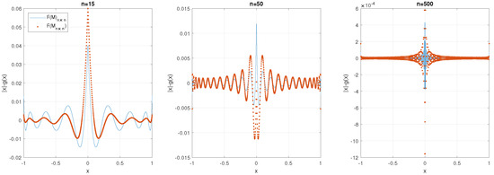
Figure 2. Error $\left|x\right|-g\left(x\right)$ with coefficients $g_j$ obtained in ${\mathsf{F}}_{n\times n}{e}_1$ and in $sign\left({\mathsf{M}}_{n\times n}\right)e_1$, with $n=15,n=50$, and $n=500$.

In Figure 3, we present in log scale the error $|g_j-F_{j,1}|$, with coefficients $g_j$ obtained with (17) and $F_{j,1}$, the values ${\mathsf{F}}_{n\times n}{e}_1$, and in matrix $sign\left({\mathsf{M}}_{n\times n}\right)e_1$, with selected values of matrix dimensions n.

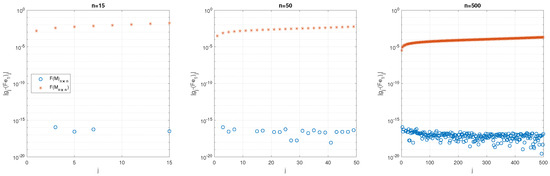
Figure 3. Error $\left|x\right|-g\left(x\right)$ with coefficients $g_j$ obtained in ${\mathsf{F}}_{n\times n}{e}_1$ and in $sign\left({\mathsf{M}}_{n\times n}\right)e_1$, with $n=15,n=50$, and $n=500$.

A similar test can be made using the fact that $P_0=1$, and so, $\mathsf{F}{e}_0=\mathsf{f}$; we can verify if ${\mathsf{F}}^{-1}\mathsf{f}=e_0$. In Figure 4, we plot the norms $\left|\right|{\mathsf{F}}^{-1}\mathsf{f}-e_0\left|\right|$, illustrating the fact that while ${\mathsf{F}}_{n\times n}^{-1}$ behaves like ${\mathsf{F}}^{-1}$, $sign{\left(\mathsf{M}\right)}_{n\times n}^{-1}$ does not. We remark that ${\mathsf{F}}_{n\times n}$ is regular for even n only.

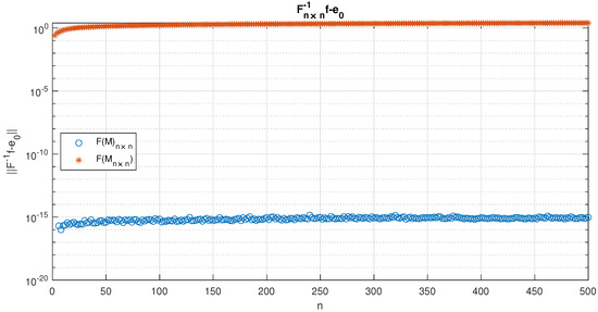
Figure 4. Norm $\left|\right|{\mathsf{F}}^{-1}\mathsf{f}-e_0\left|\right|$ for even $n=2,4,\dots ,500$.

4.2. Trigonometric Functions with Laguerre Polynomials

From the generating function of Laguerre polynomials [9],

$$e^{-ax}={\displaystyle \frac{1}{1+a}}\sum _{j=0}^{\infty }{\left({\displaystyle \frac{a}{1+a}}\right)}^j{L}_j\left(x\right)$$

we obtain

$$cos\left(x\right)=\sum _{j=0}^{\infty }{\displaystyle \frac{{(-1)}^j}{2^{2j+1}}}(L_{4j}\left(x\right)+L_{4j+1}\left(x\right)+{\displaystyle \frac{1}{2}}{L}_{4j+2}\left(x\right)).$$

The recurrence relation of Laguerre polynomials,

$$\left\{\begin{array}{c}{L}_{-1}=0,L_0=1,\hfill \\ x{L}_j=-(j+1)L_{j+1}+(2j+1)L_j-j{L}_{j-1},j=0,1,\dots ,\hfill \end{array}\right.$$

results in the particular case of recurrence relation (14):

$$\begin{array}{ccc}\hfill p_{j,i,0}& =& {\delta }_{i,j},\hfill \\ \hfill p_{j,i,1}& =& \left\{\begin{array}{cc}{\displaystyle -\frac{i}{2}(1+3{(-1)}^{j-i}),}\hfill & |j-i|\le 1,\hfill \\ 0,\hfill & |j-i|>1\hfill \end{array}\right.,\hfill \\ \hfill {\displaystyle p_{j,i,k+1}}& =& \left\{\begin{array}{cc}& {\displaystyle \frac{1}{k+1}}[i{p}_{j,i-1,k}+2(k-i)p_{j,i,k}\hfill \\ & +(i+1)p_{j,i+1,k}-k{p}_{j,i,k-1}],\hfill & & |j-i|\le k+1\hfill \\ & 0\hfill & & |j-i|>k+1\hfill \end{array}\right..\hfill \end{array}$$

Illustrating an application of these formulas, we build square matrices,

$$cos\left(\mathsf{M}\right)=\sum _{j=0}^{\infty }{\displaystyle \frac{{(-1)}^j}{2^{2j+1}}}(L_{4j}\left(\mathsf{M}\right)+L_{4j+1}\left(\mathsf{M}\right)+{\displaystyle \frac{1}{2}}{L}_{4j+2}\left(\mathsf{M}\right))$$

truncated to the respective $n\times n$ main blocks, where $\mathsf{M}$ is the Jacobi matrix of Laguerre polynomials for several values of n. Given $\mathsf{a}$, the coefficients vector of a Fourier series $y=\mathcal{L}\mathsf{a}$ in Laguerre polynomials, then $cos\left(\mathsf{M}\right)\mathsf{a}$ is the coefficients vector of $cos\left(x\right)y$ in the same polynomial basis. In order to illustrate the effectiveness of this procedure, we choose $y=x^m$, for several given m, whose Fourier–Laguerre coefficients are given by

$$x^m=\sum _{j=0}^m\left({\displaystyle \genfrac{}{}{0pt}{}{m}{j}}\right)L_j\left(x\right).$$

In Figure 5, we present in log scale the error $|x^{m}cos\left(x\right)-y_n\left(x\right)|$, for $m=4$ and $m=5$, where $y_n$ results from $cos\left(\mathsf{M}\right)\mathsf{a}$ truncated to dimension n.

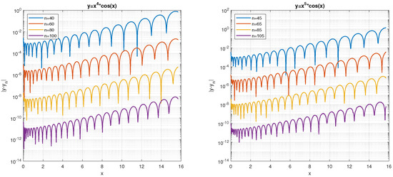
Figure 5. Absolute error $|y\left(x\right)-y_n\left(x\right)|$, for $x\in [0,5\pi ]$, with $y=x^{m}cos\left(x\right)$ for $m=4,5$; and $y_n$ is the truncated Laguerre series evaluated by truncated matrices $cos\left(\mathsf{M}\right)\mathsf{a}$.

5. Conclusions

In this work, we reveal fundamental properties of matrices resulting from the image of Jacobi matrices transformed by generalized Fourier series. These are useful matrices in the context of algebraic representation of functional operators. Among the properties associated with matrix polynomials, we highlight the relationship between linearization coefficients and operational matrices. Additionally, we explore symmetry properties, invariance over domain linear displacements, and certain recurrence relations. We conclude that the properties exhibited by matrices transformed through polynomials are inherited by matrices transformed using Fourier series with orthogonal polynomials.

In addition to efficiently addressing the challenge of operating with infinite matrices, this work offers effective calculation formulas applicable to any finite block of these matrices. The examples illustrate the successful and efficient performance of the presented calculation formulas.

References

- Gautschi, W. Orthogonal polynomials: Applications and computation. Acta Numer. 1996, 5, 45–119. [Google Scholar] [CrossRef]
- Lewanowicz, S. Second-order recurrence relation for the linearization coefficients of the classical orthogonal polynomials. J. Comput. Appl. Math. 1996, 69, 159–170. [Google Scholar] [CrossRef]
- Ronveaux, A.; Hounkonnou, M.N.; Belmehdi, S. Generalized linearization problems. J. Phys. A Math. Gen. 1995, 28, 4423. [Google Scholar] [CrossRef]
- Szwarc, R. Linearization and connection coefficients of orthogonal polynomials. Monatshefte Für Math. 1992, 113, 319. [Google Scholar] [CrossRef]
- Adams, J.C., III. On the expression of the product of any two Legendre’s coefficients by means of a series of Legendre’s coefficients. Proc. R. Soc. Lond. 1878, 27, 63–71. [Google Scholar]
- Park, S.B.; Kim, J.H. Integral evaluation of the linearization coeficients of the product of two Legendre polynomials. J. Phys. A Math. Gen. 2006, 20, 623–635. [Google Scholar]
- Chaggara, H.; Koepf, W. On linearization and connection coefficients for generalized Hermite polynomials. J. Comput. Appl. Math. 2011, 236, 65–73. [Google Scholar] [CrossRef][Green Version]
- Chaggara, H.; Koepf, W. On linearization coefficients of Jacobi polynomials. Appl. Math. Lett. 2010, 23, 609–614. [Google Scholar] [CrossRef][Green Version]
- Olver, F.W.J.; Olde Daalhuis, A.B.; Lozier, D.W.; Schneider, B.I.; Boisvert, R.F.; Clark, C.W.; Miller, B.R.; Saunders, B.V.; Cohl, H.S.; McClain, M.A. (Eds.) NIST Digital Library of Mathematical Functions. Release 1.1.10 of 2023-06-15. Available online: https://dlmf.nist.gov/ (accessed on 30 July 2024).
- Doha, E.; Abd-Elhameed, W. New linearization formulae for the products of Chebyshev polynomials of third and fourth kinds. Rocky Mt. J. Math. 2016, 46, 443–460. [Google Scholar] [CrossRef]
- Gene, H.; Golub, J.H.W. Calculation of Gauss quadrature rules. Math. Comput. 1969, 23, 221–230. [Google Scholar] [CrossRef]
- Chihara, T.S. An Introduction to Orthogonal Polynomials; Dover Publications, Inc.: Mineola, NY, USA, 2011. [Google Scholar]
- Benzi, M.; Golub, G. Bounds for the Entries of Matrix Functions with Applications to Preconditioning. BIT Numer. Math. 1999, 39, 417–438. [Google Scholar] [CrossRef]
- Abd-Elhameed, W. New product and linearization formulae of Jacobi polynomials of certain parameters. Integral Transform. Spec. Funct. 2015, 26, 586–599. [Google Scholar] [CrossRef]
- Ahmed, H.M. Computing expansions coefficients for Laguerre polynomials. Integral Transform. Spec. Funct. 2021, 32, 271–289. [Google Scholar] [CrossRef]
- Matos, J.M.A.; Rodrigues, M.J.; de Matos, J.C. Explicit formulae for derivatives and primitives of orthogonal polynomials. arXiv 2017, arXiv:1703.00743. [Google Scholar]
- Roberts, J.D. Linear model reduction and solution of the algebraic Riccati equation by use of the sign function. Int. J. Control 1980, 32, 677–687. [Google Scholar] [CrossRef]
- Wang, X.; Cao, Y. A numerically stable high-order Chebyshev-Halley type multipoint iterative method for calculating matrix sign function. AIMS Math. 2023, 8, 12456–12471. [Google Scholar] [CrossRef]
Disclaimer/Publisher’s Note: The statements, opinions and data contained in all publications are solely those of the individual author(s) and contributor(s) and not of MDPI and/or the editor(s). MDPI and/or the editor(s) disclaim responsibility for any injury to people or property resulting from any ideas, methods, instructions or products referred to in the content. |
© 2024 by the authors. Licensee MDPI, Basel, Switzerland. This article is an open access article distributed under the terms and conditions of the Creative Commons Attribution (CC BY) license (https://creativecommons.org/licenses/by/4.0/).