
Some Classical Inequalities Associated with Generic Identity and Applications
 , , ,
, , ,  and
and 
Abstract
1. Introduction
2. Main Results
2.1. Auxiliary Result
2.2. Bounds for Several Error Inequalities Involving Convex Functions
3. Visual Analysis
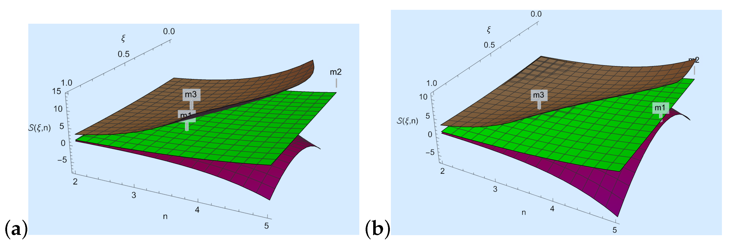
- We take , , , and in Theorem 1; then, , where
- We take , , , and in Theorem 1; then, , where
- For Figure 1a, we choose and n to develop a visual explanation of Theorem 1 at .
- For Figure 1b, we choose and n to a develop visual explanation of Theorem 1 at .
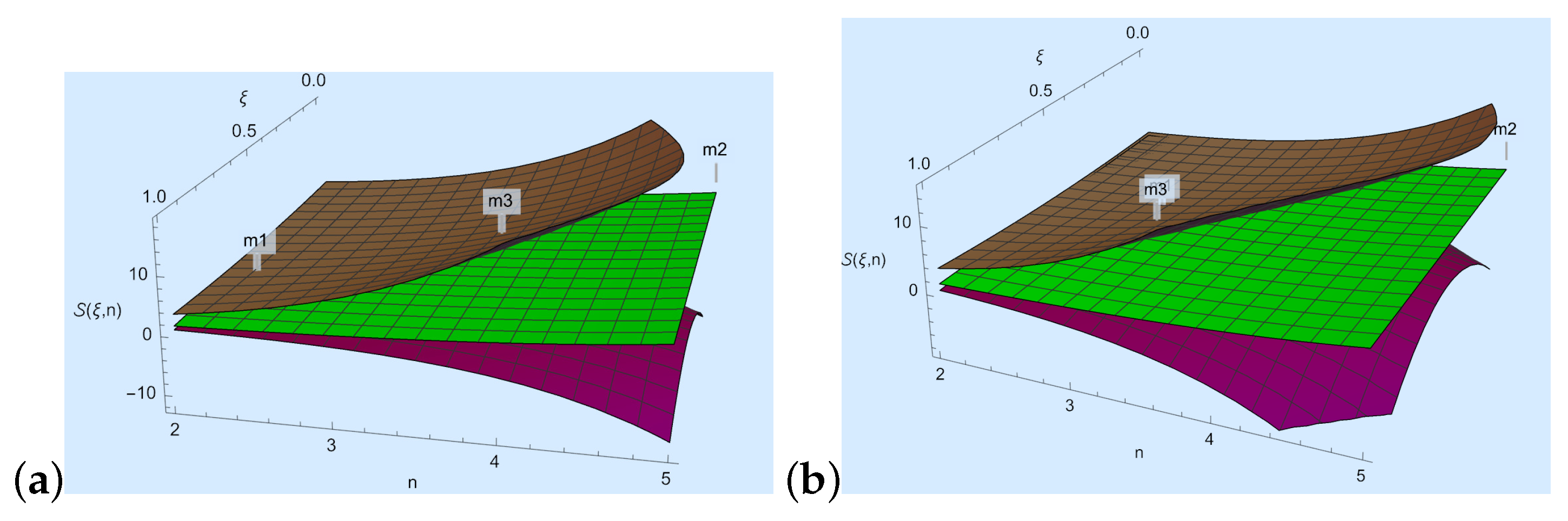
- We take , , , and in Theorem 2; then, , where
- We take , , , and in Theorem 2; then, , where
- For Figure 2a, we choose and n to develop a visual explanation of Theorem 2 at .
- For Figure 2b, we choose and n to develop a visual explanation of Theorem 2 at .
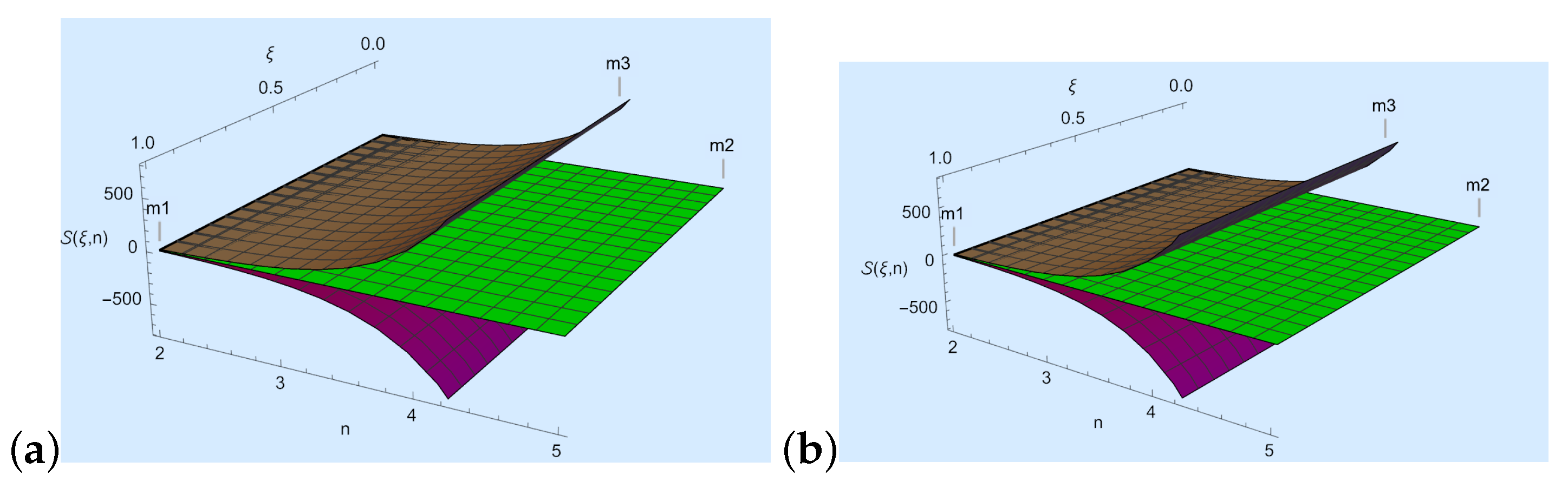
- We take , , , , and in Theorem 3; then, , where
- We take , , , , and in Theorem 3; then, , where
- For Figure 3a, we choose and n to develop a visual explanation of Theorem 3 at .
- For Figure 3b, we choose and n to develop a visual explanation of Theorem 3 at .
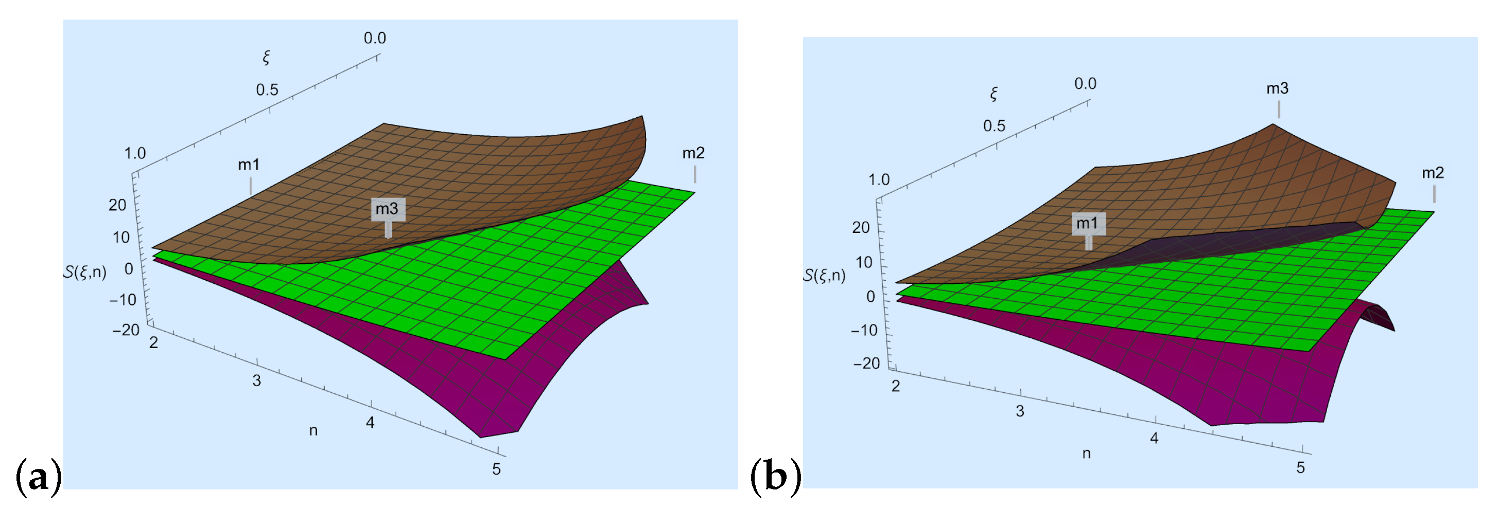
- We take , , , , and in Theorem 4; then, , where
- We take , , , and in Theorem 4, then , where
- For Figure 4a, we choose and n to develop a visual explanation of Theorem 4 at .
- For Figure 4b, we choose and n to develop a visual explanation of Theorem 4 at .
- We take , , , , and in Theorem 4; then, , where
- We take , , , , and in Theorem 5; then, , where
4. Applications
4.1. Error Boundaries of Composite Newton–Cotes Schemes
4.2. Applications for the Linear Combination of Means
- .
4.3. Application for Special Functions
4.4. Family of Iterative Methods to Find the Roots of Non-Linear Equations
- By taking in Proposition 6, we then have the following iterative schemewhere is already defined in Proposition 6.
- By taking in Proposition 6, we then have the following iterative schemewhere is already defined in Proposition 6.
- By taking in Proposition 6, we then have the following iterative schemewhere is already defined in Proposition 6.
- By taking in Proposition 6, we then have the following iterative schemewhere is already defined in Proposition 6.
- By taking in Proposition 6, we have the following iterative schemewhere is already defined in Proposition 6.
- By taking in Proposition 6, we then have the following iterative schemewhere is already defined in Proposition 6.
- It is worth noting that for different choices of γ and ξ in Theorem 5, we can generate a family of iterative methods, as well as by making use of another method in place of Newton’s method as corrector methods.
4.5. Examples and Visual Analysis of Equation (4)
- In our first example, we consider the problem related to the plug flow of Casson fluids of blood in the rheology and fractional non-linear equations model [42]. The fall in flow rate can be estimated through the following equationhere, we choose , and by selecting the initial guess of , Equation (4) with results in the required root in the third iteration.
- ,
- ,
- ,
- .
- ,
- .
| Methods | IT | ||||
| 2 | 5 | 0 | |||
| 2 | 4 | 0 | 0 | ||
| 2 | 4 | 0 | 0 | ||
| 2 | 4 | 0 | 0 | ||
| 2 | 4 | 0 | 0 |
| Methods | IT | ||||
| 6 | |||||
| 5 | 0 | ||||
| 4 | 0 | ||||
| 5 | 0 | ||||
| 5 | 0 |
| Methods | IT | ||||
| 5 | |||||
| 4 | |||||
| 4 | 0 | ||||
| 4 | 0 | ||||
| 4 | 0 |
| Methods | IT | ||||
| 2 | 4 | ||||
| 2 | 4 | ||||
| 2 | 4 | ||||
| 2 | 3 | ||||
| 2 | 4 |
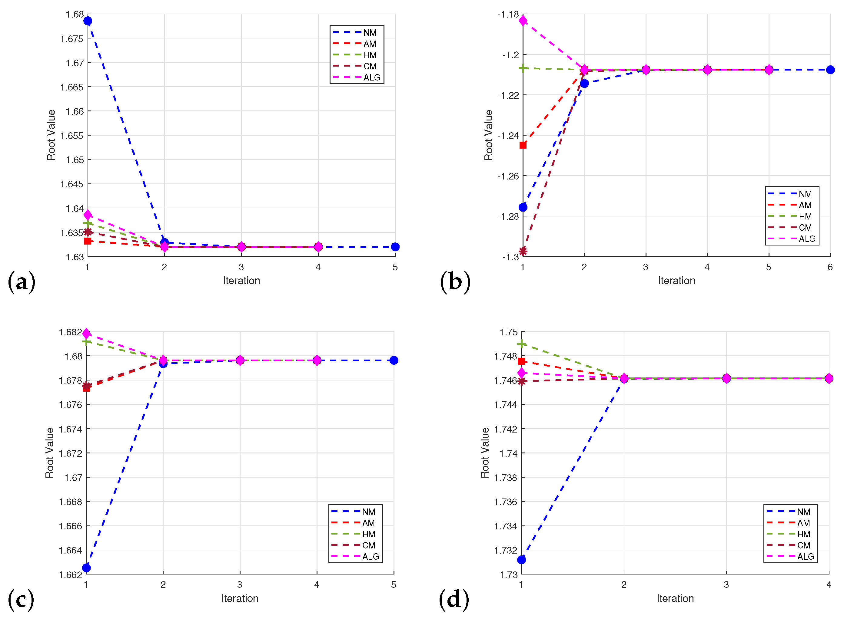
- Figure 6a describe the comparative study of our proposed Algorithm with classical schemes with respect to number of iterations and root values for .
- Figure 6b describe the comparative study of our proposed Algorithm with classical schemes with respect to number of iterations and root values for .
- Figure 6c describe the comparative study of our proposed Algorithm with classical schemes with respect to number of iterations and root values for .
- Figure 6d describe the comparative study of our proposed Algorithm with classical schemes with respect to number of iterations and root values for .
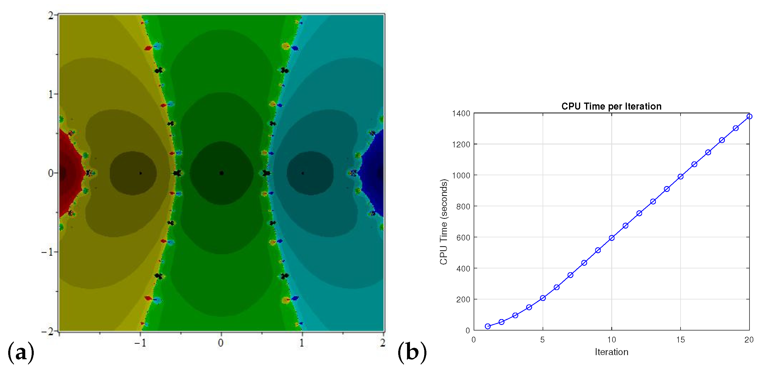
4.6. Basin of Attraction
5. Conclusions
Author Contributions
Funding
Data Availability Statement
Acknowledgments
Conflicts of Interest
References
- Dragomir, S.S.; Agarwal, R. Two inequalities for differentiable mappings and applications to special means of real numbers and to trapezoidal formula. Appl. Math. Lett. 1998, 11, 91–95. [Google Scholar] [CrossRef]
- Latif, M.A. On some inequalities for h-convex functions. Int. J. Math. Anal. 2010, 4, 1473–1482. [Google Scholar]
- Ozdemir, M.E.; Gurbuz, M.; Kavurmaci, H. Hermite-Hadamard-type inequalities for (g, ϕ, h)-convex dominated functions. J. Inequalities Appl. 2013, 2013, 184. [Google Scholar] [CrossRef]
- Abramovich, S. On superquadracity. J. Math. Inequalities 2009, 3, 329–339. [Google Scholar] [CrossRef]
- Bohner, M.; Matthews, T. Ostrowski inequalities on time scales. J. Inequalities Pure Appl. Math. 2008, 9, 8. [Google Scholar]
- Popa, E. An inequality of Ostrowski type via a mean value theorem. Gen. Math. 2007, 15, 93–100. [Google Scholar]
- Anastassiou, G.A. Univariate Ostrowski inequalities, revisited. Monatshefte Math. 2002, 135, 175–189. [Google Scholar] [CrossRef]
- Awan, M.U.; Javed, M.Z.; Budak, H.; Hamed, Y.S.; Ro, J.S. A study of new quantum Montgomery identities and general Ostrowski like inequalities. Ain Shams Eng. J. 2024, 15, 102683. [Google Scholar] [CrossRef]
- Vivas-Cortez, M.; Awan, M.U.; Asif, U.; Javed, M.Z.; Budak, H. Advances in Ostrowski-Mercer Like Inequalities within Fractal Space. Fractal Fract. 2023, 7, 689. [Google Scholar] [CrossRef]
- Dragomir, S.S.; Rassias, T.M. (Eds.) Ostrowski Type Inequalities and Applications in Numerical Integration; Kluwer Academic: Dordrecht, The Netherlands, 2002. [Google Scholar]
- Dragomir, S.S.; Agarwal, R.P.; Cerone, P. On Simpson’s inequality and applications. J. Inequalities Appl. 2000, 5, 533–579. [Google Scholar] [CrossRef]
- Liu, Z. An inequality of Simpson type. Proc. R. Soc. A Math. Phys. Eng. Sci. 2005, 461, 2155–2158. [Google Scholar] [CrossRef]
- Alomari, M.; Darus, M.; Dragomir, S.S. New inequalities of Simpson’s type for s-convex functions with applications. RGMIA Res. Rep. Collect. 2009, 4, 12. [Google Scholar]
- Sarikaya, M.Z.; Set, E.; Ozdemir, M.E. On new inequalities of Simpson’s type for s-convex functions. Comput. Math. Appl. 2010, 60, 2191–2199. [Google Scholar] [CrossRef]
- Li, Y.; Du, T. Some Simpson type integral inequalities for functions whose third derivatives are (a, m)-GA-convex functions. J. Egypt. Math. Soc. 2016, 24, 175–180. [Google Scholar] [CrossRef]
- Kashuri, A.; Mohammed, P.O.; Abdeljawad, T.; Hamasalh, F.; Chu, Y. New Simpson type integral inequalities for s-convex functions and their applications. Math. Probl. Eng. 2020, 2020, 8871988. [Google Scholar] [CrossRef]
- Fedotov, I.; Dragomir, S.S. An inequality of Ostrowski type and its applications for Simpson’s rule and special means. RGMIA Res. Rep. Collect. 1999, 2, 491–499. [Google Scholar] [CrossRef]
- Hanna, G.; Cerone, P.; Roumeliotis, J. An Ostrowski type inequality in two dimensions using the three point rule. ANZIAM J. 2000, 42, C671–C689. [Google Scholar] [CrossRef]
- Alomari, M.W.; Dragomir, S.S. Various error estimations for several Newton-Cotes quadrature formulae in terms of at most first derivative and applications in numerical integration. Jordan J. Math. Stat. 2014, 7, 89–108. [Google Scholar]
- Iftikhar, S.; Erden, S.; Ali, M.A.; Baili, J.; Ahmad, H. Simpson’s second-type inequalities for co-ordinated convex functions and applications for cubature formulas. Fractal Fract. 2022, 6, 33. [Google Scholar] [CrossRef]
- Budak, H.; Erden, S.; Ali, M.A. Simpson and Newton type inequalities for convex functions via newly defined quantum integrals. Math. Methods Appl. Sci. 2021, 44, 378–390. [Google Scholar] [CrossRef]
- Butt, S.I.; Javed, I.; Agarwal, P.; Nieto, J.J. Newton-Simpson-type inequalities via majorization. J. Inequalities Appl. 2023, 2023, 16. [Google Scholar] [CrossRef]
- Meftah, B. Maclaurin type inequalities for multiplicatively convex functions. Proc. Am. Math. Soc. 2023, 151, 2115–2125. [Google Scholar] [CrossRef]
- Peng, Y.; Du, T. Fractional Maclaurin-type inequalities for multiplicatively convex functions and multiplicatively P-functions. Filomat 2023, 37, 9497–9509. [Google Scholar] [CrossRef]
- Hezenci, H. Fractional inequalities of corrected Euler-Maclaurin-type for twice-differentiable functions. Comput. Appl. Math. 2023, 42, 92. [Google Scholar] [CrossRef]
- Alomari, M. New error estimations for the Milne’s quadrature formula in terms of at most first derivatives. Konuralp J. Math. 2013, 1, 17–23. [Google Scholar]
- Budak, H.; Kosem, P.; Kara, H. On new Milne-type inequalities for fractional integrals. J. Inequalities Appl. 2023, 2023, 10. [Google Scholar] [CrossRef]
- Bin-Mohsin, B.; Javed, M.Z.; Awan, M.U.; Khan, A.G.; Cesarano, C.; Noor, M.A. Exploration of Quantum Milne-Mercer-Type Inequalities with Applications. Symmetry 2023, 15, 1096. [Google Scholar] [CrossRef]
- Tseng, K.L.; Hwang, S.R.; Hsu, K.C. Hadamard-type and Bullen-type inequalities for Lipschitzian functions and their applications. Comput. Math. Appl. 2012, 64, 651–660. [Google Scholar] [CrossRef]
- Cakmak, M. On some Bullen-type inequalities via conformable fractional integrals. J. Sci. Perspect. 2019, 3, 285–298. [Google Scholar]
- Du, T.; Luo, C.; Cao, Z. On the Bullen-type inequalities via generalized fractional integrals and their applications. Fractals 2021, 29, 2150188. [Google Scholar] [CrossRef]
- Vivas-Cortez, M.; Javed, M.Z.; Awan, M.U.; Noor, M.A.; Dragomir, S.S. Bullen-Mercer type inequalities with applications in numerical analysis. Alex. Eng. J. 2024, 96, 15–33. [Google Scholar] [CrossRef]
- Xi, B.Y.; Qi, F. Some Integral Inequalities of Hermite-Hadamard Type for Convex Functions with Applications to Means. J. Funct. Spaces 2012, 2012, 980438. [Google Scholar] [CrossRef]
- Nwaeze, E.R.; Tameru, A.M. New parameterized quantum integral inequalities via η-quasiconvexity. Adv. Differ. Equ. 2019, 2019, 425. [Google Scholar] [CrossRef]
- Du, T.; Yuan, X. On the parameterized fractal integral inequalities and related applications. Chaos Solitons Fractals 2023, 170, 113375. [Google Scholar] [CrossRef]
- Yu, Y.; Liu, J.; Du, T. Certain error bounds on the parameterized integral inequalities in the sense of fractal sets. Chaos Solitons Fractals 2022, 161, 112328. [Google Scholar] [CrossRef]
- Nonlaopon, K.; Awan, M.U.; Talib, S.; Budak, H. Parametric generalized (p, q)-integral inequalities and applications. AIMS Math. 2022, 7, 12437–12457. [Google Scholar] [CrossRef]
- Kirmaci, U.S. Inequalities for differentiable mappings and applications to special means of real numbers and to midpoint formula. Appl. Math. Comput. 2004, 147, 137–146. [Google Scholar] [CrossRef]
- Raees, M.; Anwar, M.; Vivas-Cortez, M.; Kashuri, A.; Samraiz, M.; Rahman, G. New simpson’s type estimates for two newly defined quantum integrals. Symmetry 2022, 14, 548. [Google Scholar] [CrossRef]
- Watson, G.N. A Treatise on the Theory of Bessel Functions; Cambridge University Press: Cambridge, UK, 1922; Volume 2. [Google Scholar]
- Luke, Y.L. (Ed.) Special Functions and Their Approximations; Academic Press: Cambridge, MA, USA, 1969. [Google Scholar]
- Fournier, R.L. Basic Transport Phenomena in Biomedical Engineering; CRC Press: Boca Raton, FL, USA, 2017. [Google Scholar]
- Burden, R.K.; Faires, J.D. Numerical Analysis, 9th ed.; Brooks/Cole; Cengage Learning: Boston, MA, USA, 2011. [Google Scholar]
- Abbasbandy, S. Improving Newton-Raphson method for nonlinear equations by modified Adomian decomposition method. Appl. Math. Comput. 2003, 145, 887–893. [Google Scholar] [CrossRef]
- Chun, C. Iterative methods improving Newton’s method by the decomposition method. Comput. Math. Appl. 2005, 50, 1559–1568. [Google Scholar] [CrossRef]


Disclaimer/Publisher’s Note: The statements, opinions and data contained in all publications are solely those of the individual author(s) and contributor(s) and not of MDPI and/or the editor(s). MDPI and/or the editor(s) disclaim responsibility for any injury to people or property resulting from any ideas, methods, instructions or products referred to in the content. |
© 2024 by the authors. Licensee MDPI, Basel, Switzerland. This article is an open access article distributed under the terms and conditions of the Creative Commons Attribution (CC BY) license (https://creativecommons.org/licenses/by/4.0/).
Share and Cite
Javed, M.Z.; Awan, M.U.; Bin-Mohsin, B.; Budak, H.; Dragomir, S.S. Some Classical Inequalities Associated with Generic Identity and Applications. Axioms 2024, 13, 533. https://doi.org/10.3390/axioms13080533
Javed MZ, Awan MU, Bin-Mohsin B, Budak H, Dragomir SS. Some Classical Inequalities Associated with Generic Identity and Applications. Axioms. 2024; 13(8):533. https://doi.org/10.3390/axioms13080533
Chicago/Turabian StyleJaved, Muhammad Zakria, Muhammad Uzair Awan, Bandar Bin-Mohsin, Hüseyin Budak, and Silvestru Sever Dragomir. 2024. "Some Classical Inequalities Associated with Generic Identity and Applications" Axioms 13, no. 8: 533. https://doi.org/10.3390/axioms13080533
APA StyleJaved, M. Z., Awan, M. U., Bin-Mohsin, B., Budak, H., & Dragomir, S. S. (2024). Some Classical Inequalities Associated with Generic Identity and Applications. Axioms, 13(8), 533. https://doi.org/10.3390/axioms13080533