Article

Fox’s H-Functions: A Gentle Introduction to Astrophysical Thermonuclear Functions

1
Office for Outer Space Affairs, Vienna International Centre, 1400 Vienna, Austria
2
Department of Mathematics, University of Kerala, Kariavattom, Thiruvananthapuram 695581, India
*
Author to whom correspondence should be addressed.
Axioms 2024, 13(8), 532; https://doi.org/10.3390/axioms13080532
Submission received: 9 July 2024 / Revised: 4 August 2024 / Accepted: 5 August 2024 / Published: 6 August 2024

Abstract

:
Needed for cosmological and stellar nucleosynthesis, we are studying the closed-form analytic evaluation of thermonuclear reaction rates. In this context, we undertake a comprehensive analysis of three largely distinct velocity distributions, namely the Maxwell–Boltzmann distribution, the pathway distribution, and the Mittag-Leffler distribution. Moreover, a natural generalization of the Maxwell–Boltzmann velocity distribution is discussed. Furthermore, an explicit evaluation of the reaction rate integral in the high-energy cut-off case is carried out. Generalized special functions of mathematical physics like Meijer’s G-function and Fox’s H-functions and their utilization in mathematical physics are the prime focus of this paper.

1. Fox’s H -Functions

The invention of G- and H-functions has created a revolution in special function theory, as these are two functions that are general in nature, covering the genesis of many special functions, and have wide applicability. C. S. Meijer, in 1936 [1], introduced the G-function as a generalization of the hypergeometric function in terms of the Mellin–Barnes contour integral. Following the definition of Meijer’s G-function, in 1961, Charles Fox [2] defined a new function involving the Mellin–Barnes integrals covering Meijer’s G-function, which he called H ( x ) , later known as the H-function. The H-function turns out to be a generalization of many known special functions at that time, namely hypergeometric functions, Wright functions, Mittag-Leffler functions, Bessel functions, G-functions, etc.
Fox’s H-function is defined for integers m ,   n ,   a ,   b by 0 m b , 0 n a , and c i , d j C and for C i , D j R + = ( 0 , ) by
H a , b m , n ( z | ( c 1 , C 1 ) , , ( c a , C a ) ( d 1 , D 1 ) , , ( d b , D b ) ) : = 1 2 π i C Φ ( w ) z w d w
Φ ( w ) = j = 1 m Γ ( d j + D j w ) j = 1 n Γ ( 1 c j C j w ) j = m + 1 b Γ ( 1 d j D j w ) j = n + 1 a Γ ( c j + C j w )
where
z w = exp [ w { ln | z | + arg z } ] ; z 0 ; i = 1 ;
where arg ( z ) is not necessarily the principal value. Here C is an appropriate contour separating the poles
ζ j l = d j + l D j , j = 1 , 2 , , m ; l = 0 , 1 , 2 ,
of Γ ( d j + D j w ) , j = 1 , , m from those poles
η i k = 1 c i + k C i , i = 1 , 2 , , n ; k = 0 , 1 , 2 ,
of Γ ( 1 c i C i w ) , i = 1 , , n . We assume that no poles of Γ ( d j + D j s ) for j = 1 , 2 , , m coincide with any poles of Γ ( 1 c j C j w ) for j = 1 , 2 , , n , where Γ ( · ) denotes the gamma function that for ( λ ) > 0 ,   Γ ( λ ) = 0 t λ 1 exp t d t , due to Euler. Details on the different types of contours for C and the convergence conditions of their existence is available in numerous books, see for example Mathai et al. [3], Kilbas and Saigo [4,5], Prudnikov et al. [6], etc. Let
Δ = j = 1 b D j i = 1 a C i a * = i = 1 n C i i = n + 1 a C i + j = 1 m D j j = n + 1 b D j μ * = j = 1 b d j i = 1 a c i + a b 2 δ * = i = 1 a C i C i j = 1 b D j D j ,
then the existence conditions for Fox’s H-function are given by the following cases [4]:
1 . C = C , Δ > 0 , z 0 , 2 . C = C , Δ = 0 , 0 < | z | < δ * , 3 . C = C , Δ = 0 , | z | = δ * , ( μ * ) < 1 ,
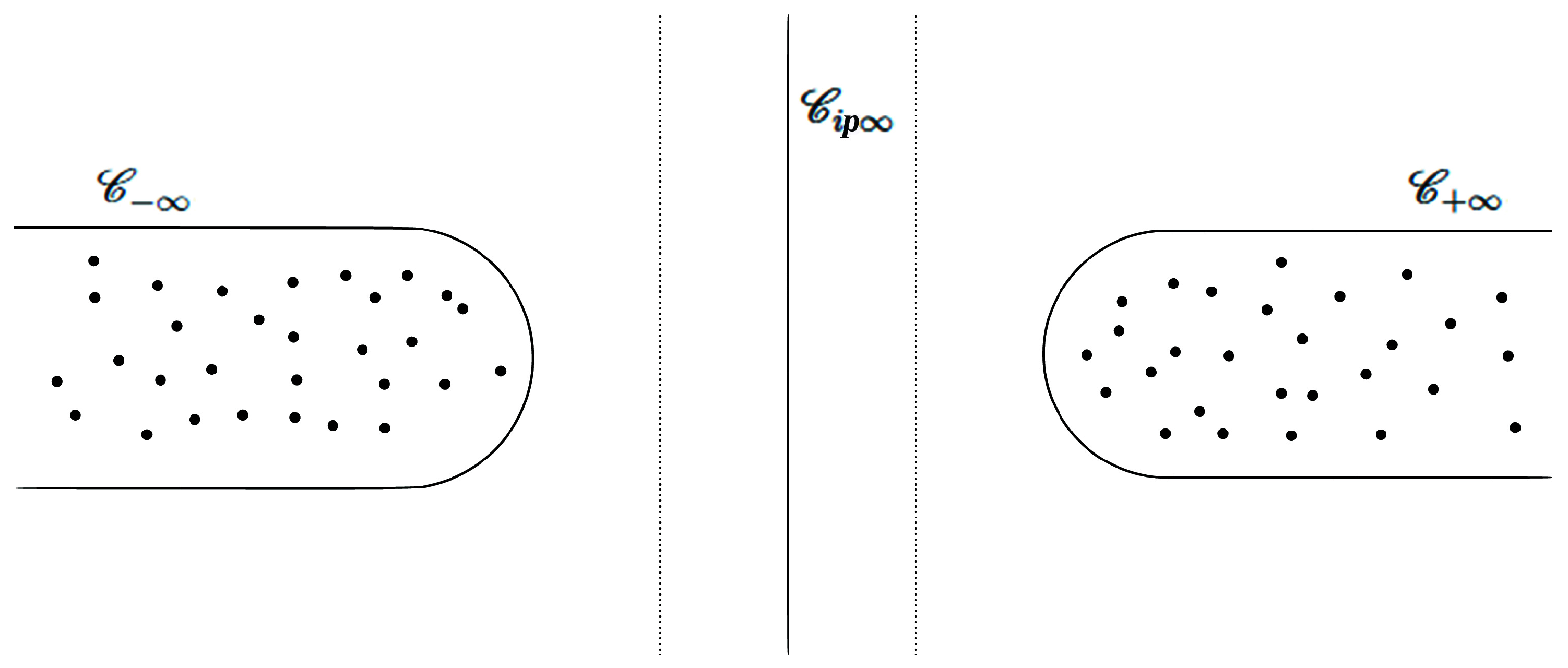
where the notation C is used to represent the left loop beginning at + i λ 1 and ending at + i λ 2 , < λ 1 < λ 2 < ; see Figure 1. Further,
4 . C = C + , Δ < 0 , z 0 , 5 . C = C + , Δ = 0 , | z | > δ * , 6 . C = C + , Δ = 0 , | z | = δ * , ( μ * ) < 1 ,
where C + is a right loop starting at + + i λ 1 and terminating at + + i λ 2 , < λ 1 < λ 2 < . Also,
7 . C = C i p , a * > 0 , | arg z | < a * π 2 8 . C = C i p , a * = 0 , Δ p + ( μ * ) < 1 , arg z = 0 , z 0 ,
where C i p is a contour starting at p i and terminating at p + i , p R ; see Figure 1. For suitable restrictions for the parameters, in particular
min 1 j m d j D j < ( w ) < min 1 i n 1 c i C i ,
a * > 0 , | arg z | < a * π 2 , z 0 ; thus, it is evident that the Mellin transformation of H a , b m , n ( z | ( c 1 , C 1 ) , , ( c a , C a ) ( d 1 , D 1 ) , , ( d b , D b ) )   is Φ (w).
Figure 1. Different types of contours for Fox’s H-function.
Axioms 13 00532 g001
For instance, setting C i , D j = E , E > 0 for i = 1 , 2 , , a and j = 1 , 2 , , b in the above definition of the H-function, we obtain the Meijer G-function, defined as
G a , b m , n ( z 1 E | c 1 , , c a d 1 , , d b ) : = E 2 π i C ϕ ( w ) z w d w
Here,
ϕ ( w ) = j = 1 m Γ ( d j + w ) j = 1 n Γ ( 1 c j w ) j = m + 1 b Γ ( 1 d j w ) j = n + 1 a Γ ( c j + w ) ,
and C is the suitable contour. The existence conditions for the G-function can be found from the above existence condition for Fox’s H-function.
There are numerous generalizations of Fox’s H-function that have been developed by many authors; see, for example [7,8,9]. However, we are not going to discuss all such generalizations, but rather the following: in 2018, Srivastava et al. [10] introduced a family of incomplete H-functions by means of the incomplete gamma functions, namely, the lower gamma function
γ λ , z : = 0 z t λ 1 exp t d t , ( λ ) > 0 , z 0
and the upper gamma function
Γ λ , z : = z t λ 1 exp t d t , z 0 ; ( λ ) > 0 , if z = 0 .
The incomplete H-functions, according to Srivastava et al. [10], are the following:
H ̲ a , b m , n ( z | ( c 1 , C 1 , y ) , ( c 2 , C 2 ) , , ( c a , C a ) ( d 1 , D 1 ) , , ( d b , D b ) ) : = 1 2 π i C Φ 1 ( w , y ) z w d w
and
H ̲ a , b m , n ( z | ( c 1 , C 1 , y ) , ( c 2 , C 2 ) , , ( c a , C a ) ( d 1 , D 1 ) , , ( d b , D b ) ) : = 1 2 π i C Φ 2 ( w , y ) z w d w
Here,
Φ 1 ( w ) = γ 1 c 1 C 1 w , y j = 1 m Γ ( d j + D j w ) j = 2 n Γ ( 1 c j C j w ) j = m + 1 b Γ ( 1 d j D j w ) j = n + 1 a Γ ( c j + C j w )
and
Φ 2 ( w ) = Γ 1 c 1 C 1 w , y j = 1 m Γ ( d j + D j w ) j = 2 n Γ ( 1 c j C j w ) j = m + 1 b Γ ( 1 d j D j w ) j = n + 1 a Γ ( c j + C j w ) .
The incomplete H-functions H ¯ a , b m , n ( · ) and H ̲ a , b m , n ( · ) exist for all y 0 under the same conditions stated above. One can readily find that H ¯ a , b m , n ( · ) + H ̲ a , b m , n ( · ) = H a , b m , n ( · ) . For more details we refer readers to [10].
This article is setup in the following way: Section 2 defines thermonuclear fusion reaction rates in high-energy physics. In Section 3, we demonstrate how the Maxwell–Boltzmann distribution affects reaction rates in solar analogs, specifically in resonant reaction or direct capture cases. We also discuss a natural generalization of the Maxwell–Boltzmann distribution. Section 4 and Section 5 describe non-perfect situations, such as non-equilibrium hydrostatic conditions that arise or non-Maxwellian cases due to practical disturbances. In such cases, the pathway model or Mittag-Leffler Gaussian model are employed to obtain the reaction rates in a closed form. Additionally, a closed-form evaluation of the reaction rate integral in the cut-off scenario is performed. Section 6 includes a comparative analysis of the velocity distributions along with our concluding remarks.

2. Thermonuclear Reactions

The sun and other stars are governed by explosive thermonuclear fusion processes. These reactions involve the collision of atomic nuclei at incredibly high temperatures, typically millions of degrees Celsius, found in a star’s core. In such extreme conditions, the velocity distribution of the interacting particles is governed by the principles of plasma physics. For those charged particles, the Maxwell–Boltzmann velocity distribution describes how particles within the plasma move and collide. Understanding this distribution is crucial, as it dictates the likelihood of particles having sufficient kinetic energy to overcome electrostatic repulsion and engage in nuclear fusion. Essentially, the velocity distribution of particles drives the reaction rates and probabilities of thermonuclear reactions, determining the star’s energy output and, ultimately, its lifespan. Nuclear fusion reactions not only produce the energy that powers the evolution of stars but also contribute to the creation of elements in the universe. These processes primarily involve reactions driven by hydrogen, helium, neutrons, and heavy ions such as carbon and oxygen [11].
In a non-degenerate setting, for particles of type i and j, r i j denotes the reaction rate, which is given by [12]:
r i j = n i n j σ i j v .
Here, n i represents the number density of particle of type i and n j represents the number density of particle of type j. The relative velocity v and the energy-dependent reaction cross-section σ ( v ) of the interacting particles are combined to obtain an appropriate average σ i j v , which is given by
σ i j v = 0 v f ( v ) σ ( v ) d 3 v ,
where f ( v ) is the distribution function of the relative velocity of the particles i , j and d 3 v = 4 π v 2 d v . In terms of energy E, the reaction cross-section σ ( E ) can be parametrized by the S-factor S ( E ) using the relation
σ ( E ) = S ( E ) E exp 2 π η ( E ) ,
where
η ( E ) = μ 2 1 2 z i z j e 2 1 E 1 2
is the Sommerfeld parameter, is Plank’s quantum of action, e is the quantum of electric charge, and z i and z j denote the charges of the interacting particles. A better approximation to S ( E ) is a Maclaurin series up to the second order of E
S ( E ) S ( 0 ) + d d E S ( 0 ) E + 1 2 ! d d E S ( 0 ) E 2 = ν = 0 2 S ν ( 0 ) ν ! E ν .

3. Maxwell–Boltzmann Case

The Maxwell–Boltzmann distribution is a fundamental concept that describes the distribution of particle velocities within a high-temperature environment, such as the core of a star. In this distribution, particles like protons and helium nuclei exhibit a wide range of velocities due to their thermal motion. Some particles possess energies and velocities high enough to overcome the Coloumb barrier and successfully collide, initiating nuclear fusion. The Maxwell–Boltzmann distribution helps us understand the probability of different particles having the necessary kinetic energy for fusion events, which is vital for comprehending the rates and efficiencies of the thermonuclear reactions that power the stars and drive the energy balance within celestial objects. Under a non-relativistic, non-degenerate setup, these particles follow the classical Maxwell–Boltzmann velocity distribution when they are in thermodynamic equilibrium, which is given by [12]:
f M B D ( v ) d v = μ 2 π K B T 3 2 exp μ v 2 2 K B T 4 π v 2 d v .
Here, the reduced mass of the reacting particles is denoted by μ , the temperature of the system is represented by T, and K B denotes Boltzmann’s constant. The classical Maxwell–Boltzmann energy distribution corresponds to (10) and can be obtained as
f M B D ( E ) d E = 2 π 1 π K B T 3 2 exp E K B T E d E ,
where E is the kinetic energy, E = 1 2 μ v 2 .
For particles moving at relativistic speeds, their kinetic energy may differ significantly from the classical expression 1 2 μ v 2 . For example, when we consider particles which move at a speed close to the speed of light, their kinetic energy can be described by relativistic mechanics rather than 1 2 μ v 2 . In such cases, their relativistic kinetic energy is given by
E k i n e t i c = ( γ 1 ) μ C 2 .
Here, γ denotes the Lorentz factor and C is the speed of light. In a similar way, quantum systems may also deviate from the classical energy relation. Likewise, in high-energy physics, particles can possess extremely high kinetic energies and show deviation from 1 2 μ v 2 . Particularly in astrophysical contexts, such as within the sun or other stars, particles can attain extremely high energies and behave like non-classical systems. For this reason, here we consider the energy function in a more general form,
E ( v ) = A f ( v ) ,
where f ( v ) is any function of velocity v and A denotes the scaling factor. In particular, let us define
E ( v ) = A v 2 p , ( p > 0 ) .
Using (14) with the scaling factor μ 2 , one can write the generalized Maxwell–Boltzmann velocity distribution as
f G M B ( v ) d v = p Γ 3 2 p μ 2 K B T 3 2 p v 2 exp μ v 2 p 2 K B T d v ( p > 0 ) .
It is readily seen that (15) is an immediate generalization of (10). In terms of energy E,
f G M B ( E ) d E = 1 Γ 3 2 p 1 2 K B T 3 2 p exp E K B T 2 E 3 2 p 1 d E ( p > 0 ) .
Using (6) and (16), we obtain the reaction rate in the generalized Maxwell–Boltzmann case, as
r i j ( p ) = n i n j 2 1 2 p Γ 3 2 p 1 K B T 3 2 p 1 μ 1 2 p 0 E 2 p 1 σ ( E ) exp E K B T d E .
Now, using (7) and (9), we have
r i j ( p ) = n i n j Γ 3 2 p 1 K B T 3 2 p 2 μ 1 2 p ν = 0 2 S ( ν ) ( 0 ) ν ! 0 E ν exp E K B T 2 π μ 2 1 2 z i z j e 2 E 1 2 d E .
Taking t = E K B T and x = 2 π μ 2 1 2 z i z j e 2 , we have the simplified form of the reaction rate:
r i j ( p ) = n i n j Γ 3 2 p 1 K B T 3 2 p 2 μ 1 2 p ν = 0 2 S ( ν ) ( 0 ) ν ! 0 t ν exp t x t 1 2 d t .
Using the Meijer G-function, one can end up with the following closed expression of the non-resonant reaction rate in the generalized Maxwell–Boltzmann case:
r i j ( p ) = n i n j Γ 3 2 p 1 K B T 3 2 p 2 μ 1 2 p ν = 0 2 S ( ν ) ( 0 ) ν ! G 0 , 3 3 , 0 ( x 2 4 | 0 , 1 2 , ν + 1 ) ,
where p > 0 .
For instance, when p = 1 , both energy distributions in (16) and (11) coincide. That is, for x = 2 π μ 2 1 2 z i z j e 2 , the standard reaction rate in the classical Maxwell–Boltzmann case can be obtained as
r i j = n i n j π 8 μ 1 2 ν = 0 2 S ( ν ) ( 0 ) ν ! 1 K B T ν + 1 2 G 0 , 3 3 , 0 ( x 2 4 | 0 , 1 2 , ν + 1 ) ,
This evaluation can be found in the recent literature; see, for example, [13]. It is clear that there is no explicit difference between the reaction rate integrals in classical Maxwell–Boltzmann and generalized Maxwell–Boltzmann cases.
During reactions, a high-energy tail cut-off may occur due to various factors, which results in a modified energy distribution. In such cases, the reaction rate in the classical Maxwell–Boltzmann case becomes
C r i j = n i n j π 8 μ 1 2 ν = 0 2 1 K B T ν + 1 2 S ( ν ) ( 0 ) ν ! 0 d y ν exp y x y 1 2 d y ,
where d < is the cut-off parameter. In order to evaluate the cut-off reaction rate C r i j in (21), consider the reaction rate integral explicitly, as
g ( x ) = 0 d y ν exp y x y 1 2 d y .
Since g ( x ) is a complex valued function of the real positive variable x, we can apply the one-variable Mellin transform to (22) and find that
M g ( x ) ( s ) = 0 x s 1 0 d y ν exp y x y 1 2 d y d x .
Interchanging the integral and making use of the gamma and lower gamma functions, we have
M g ( x ) ( s ) = Γ ( s ) 0 d y ν + s 2 exp y d y .
With further simplifications, we obtain
M g ( x ) ( s ) = Γ ( s ) γ ν + s 2 + 1 , d , ( ( s ) > 0 ) .
Taking the inverse Mellin transform, one can find that
g ( x ) = 1 2 π i C γ 1 + ν w 2 , d Γ ( w ) 1 x w d w .
Using the incomplete H-function in (4), we know that
g ( x ) = H ̲ 2 , 0 0 , 2 ( 1 x | ( ν , 1 2 , d ) , ( 1 , 1 ) )
Hence, according to (21), we obtain the reaction rate in the cut-off case:
C r i j = n i n j π 8 μ 1 2 ν = 0 2 1 K B T ν + 1 2 S ( ν ) ( 0 ) ν ! H ̲ 2 , 0 0 , 2 ( 1 x | ( ν , 1 2 , d ) , ( 1 , 1 ) ) .
One might imagine an alternate velocity distribution in place of the Maxwell–Boltzmann distribution for the nuclear fusion processes occurring in star interiors if there is a deviation from hydrostatic equilibrium. The following sections discuss more alternative distributions which also cover the classical Maxwell–Boltzmann distribution.

4. Pathway Case

In 2005, Mathai [14] introduced a statistical model into the matrix variate case that is called the pathway model. In a real scalar one-variable situation, the representation of the pathway model P ( t ) is as follows:
P ( t ) = N 1 | t | ν 1 [ 1 x ( 1 β ) | t | δ ] η 1 β , x > 0 , δ > 0 , 1 x ( 1 β ) | t | δ > 0 , ν > 0 , η > 0 .
where β denotes the pathway parameter. When β < 1 , the model in (29) belongs to the generalized type-1 beta form of real scalar cases. When β > 1 ,
P ( t ) = N 2 | t | ν 1 [ 1 + x ( β 1 ) | t | δ ] η 1 β ,
belongs to the generalized type-2 beta family of real scalar cases. When β 1 , the two forms in (29) and (30) reduce to the gamma form
P ( t ) = N 3 | t | ν 1 exp x η | t | δ .
Several statistical densities can be viewed as specific instances of one of the three pathway functional forms mentioned above; see [14]. Notice that N 1 , N 2 , and N 3 are the normalizing constants.
In 2018, Haubold and Kumar [12] extended the thermonuclear integrals by utilizing Mathai’s pathway idea for real scalar cases [14], covering the non-extensive statistical mechanics of Tsallis [15]. They also represented extended reaction rates in the form of Fox’s H-function. The pathway energy distribution considered by Haubold and Kumar [12] is given by
f P D ( E ) d E = 2 π ( β 1 ) 3 2 ( π K B T ) 3 2 Γ 1 β 1 Γ 1 β 1 3 2 E 1 + ( β 1 ) E K B T 1 β 1 d E ,
where β > 1 , 1 β 1 > 3 2 . Using (6), the standard reaction rate in the pathway case is given by
r ˜ i j = n i n j 8 μ π 1 2 ( β 1 K B T ) 3 2 Γ 1 β 1 Γ 1 β 1 3 2 ν = 0 2 S ( ν ) ( 0 ) ν ! 0 E ν 1 + ( β 1 ) E K B T 1 β 1 × exp 2 π μ 2 1 2 z i z j e 2 E 1 2 d E ,
which, in closed form, leads to
r ˜ i j = n i n j 8 μ π 1 2 ( β 1 ) 3 2 Γ 1 β 1 3 2 ν = 0 2 1 K B T ν + 1 2 S ( ν ) ( 0 ) ν ! 1 ( β 1 ) ν + 1 × G 1 , 3 3 , 1 ( x 2 ( β 1 ) 4 | 2 1 β 1 + ν 0 , 1 2 , ν + 1 ) .
By setting E = 1 2 μ v 2 in (32), the corresponding velocity distribution in the extended pathway case is given by
f P D ( v ) d v = ( β 1 ) μ 2 π K B T 3 2 Γ 1 β 1 Γ 1 β 1 3 2 1 + ( β 1 ) μ v 2 2 K B T 1 β 1 4 π v 2 d v .
As β approaches to 1, one can retrieve the Maxwell–Boltzmann case.
Let us consider the cut-off case integral in its pathway form. Using the type-1 pathway form, one can write the reaction rate integral in the cut-off case as
f ˜ ( x ) = 0 1 y ( 1 β ) t ν 1 y ( 1 β ) t 1 1 β exp x t 1 2 d t , β < 1 , y > 0 .
Making the use of Mellin transform of one variable,
M f ˜ ( x ) ( s ) = 0 x s 1 exp x t 1 2 0 1 y ( 1 β ) t ν 1 y ( 1 β ) t 1 1 β d t d x .
Using the type-1 beta and gamma functions, we obtain
M f ˜ ( x ) ( s ) = 1 y 1 β s 2 + ν + 1 Γ ( s ) Γ s 2 + ν + 1 Γ 1 + 1 1 β Γ s 2 + ν + 2 + 1 1 β .
Therefore, for β < 1 ,
f ˜ ( x ) = Γ 1 + 1 1 β y 1 β ν + 1 H 1 , 2 2 , 0 ( x y ( 1 β ) 1 2 | 1 + ν , 1 2 , ( 0 , 1 ) 2 + ν + 1 1 β , 1 2 ) .
Using (39), one can find the reaction rate in the cut-off case in its closed form.

5. Mittag-Leffler Case

The Mittag-Leffler function, a special function of mathematical physics, can describe many complex behaviors and phenomena as it is a generalization of the exponential function. Haubold et al. introduced the Mittag-Leffler velocity distribution for 0 < α 1 in the form
f M L ( v ) d v = Γ 1 α 2 α π μ 2 π K B T 3 2 E α , α μ v 2 2 K B T 4 π v 2 d v ,
using the one-parameter standard Mittag-Leffler Gaussian distribution studied by Agahi and Alipour [16] (2.2). Here, E α , α ( · ) is the Mittag-Leffler function [17]:
E α , α ( z ) = k = 0 z k Γ ( α k + α ) , z , α C , ( α ) > 0 .
The energy distribution corresponding to (40) is given by
f M L ( E ) d E = 2 π α Γ 1 α 2 1 π K B T 3 2 E α , α E K B T E d E ,
where 0 < α 1 , which, in terms of the H-function, is
r i j = n i n j 8 μ 1 2 Γ 1 α 2 α π ν = 0 2 1 K B T ν + 1 2 S ( ν ) ( 0 ) ν ! z ν + 1 × H 1 , 3 2 , 1 ( x | ν + 1 , 1 2 ( 0 , 1 ) , ν + 1 , 1 2 , ( 1 α + α ν + α , α 2 ) ) .
The detailed evaluation procedure of the above integral is provided in Appendix A.
In the cut-off case, the reaction rate becomes
r i j * = n i n j 8 μ 1 2 Γ 1 α 2 α π ν = 0 2 1 K B T ν + 1 2 S ( ν ) ( 0 ) ν ! 0 d y ν E α , α y exp x y 1 2 d y ,
where d is the cut-off parameter. The evaluation of the integral results in Meijer’s G-function, as
C r i j * = n i n j 8 μ 1 2 Γ 1 α 2 α π ρ ν = 0 2 1 K B T ν + 1 2 × S ( ν ) ( 0 ) d ν ν ! z ν + 1 m = 0 ( 1 ) m ( z d ) m Γ ( α m + α ) G 1 , 3 3 , 0 ( x 2 4 d | m + ν + 2 m + ν + 1 , 0 , 1 2 )       ( d < )
The detailed evaluation procedure of the above integral is given in Appendix A.

6. Interpretations and Concluding Remarks

In the present scenario, we undertook a comprehensive study of velocity distributions, namely, the Maxwell–Boltzmann, the pathway, and the Mittag-Leffler distributions.
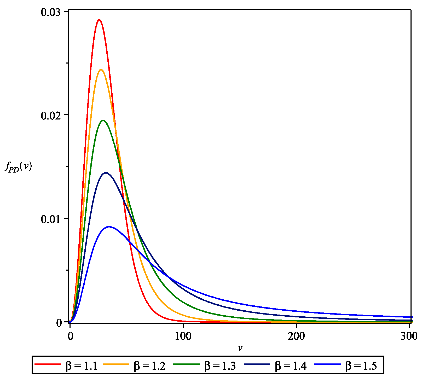
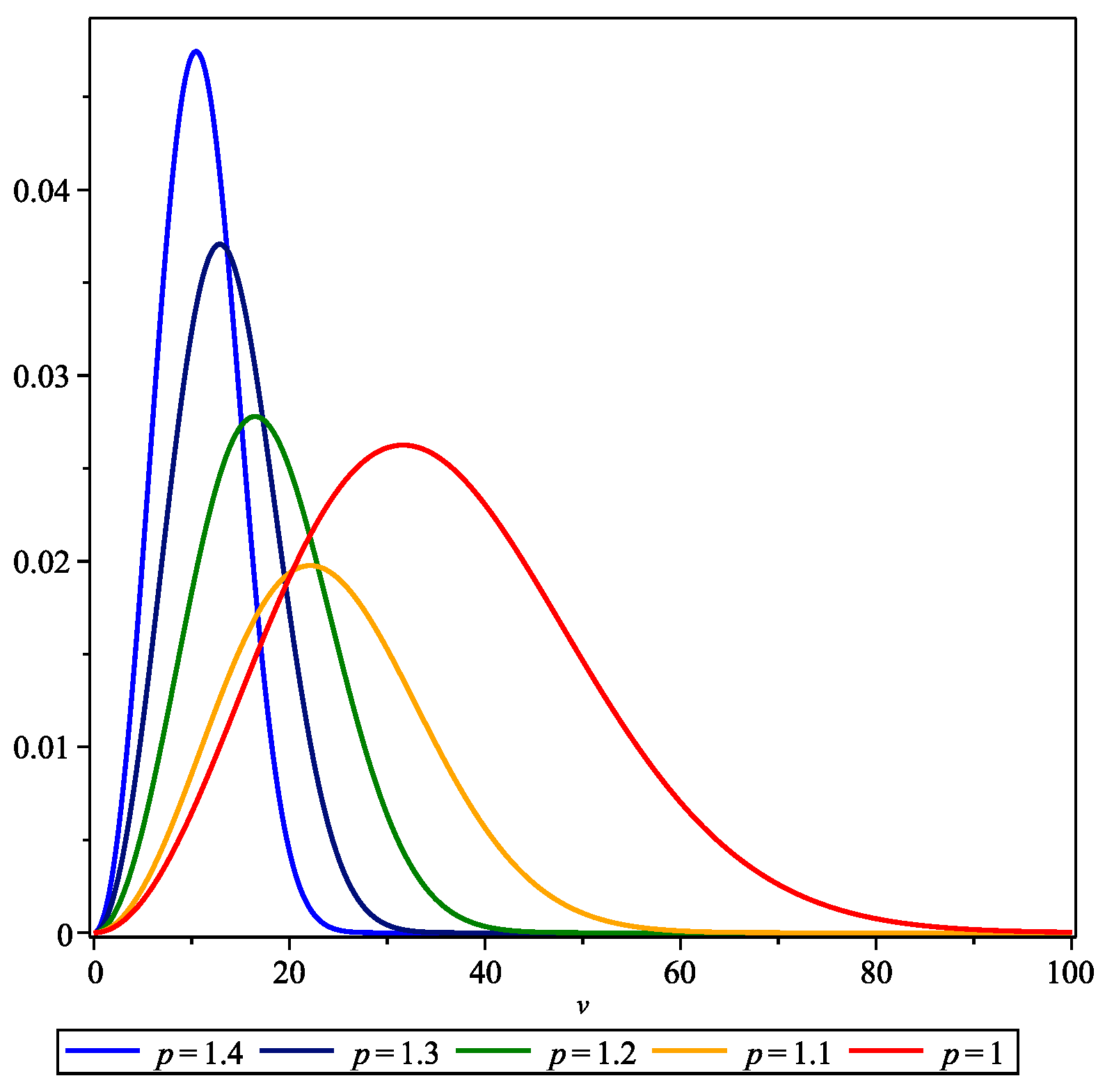
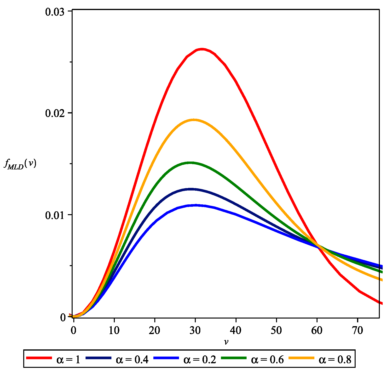
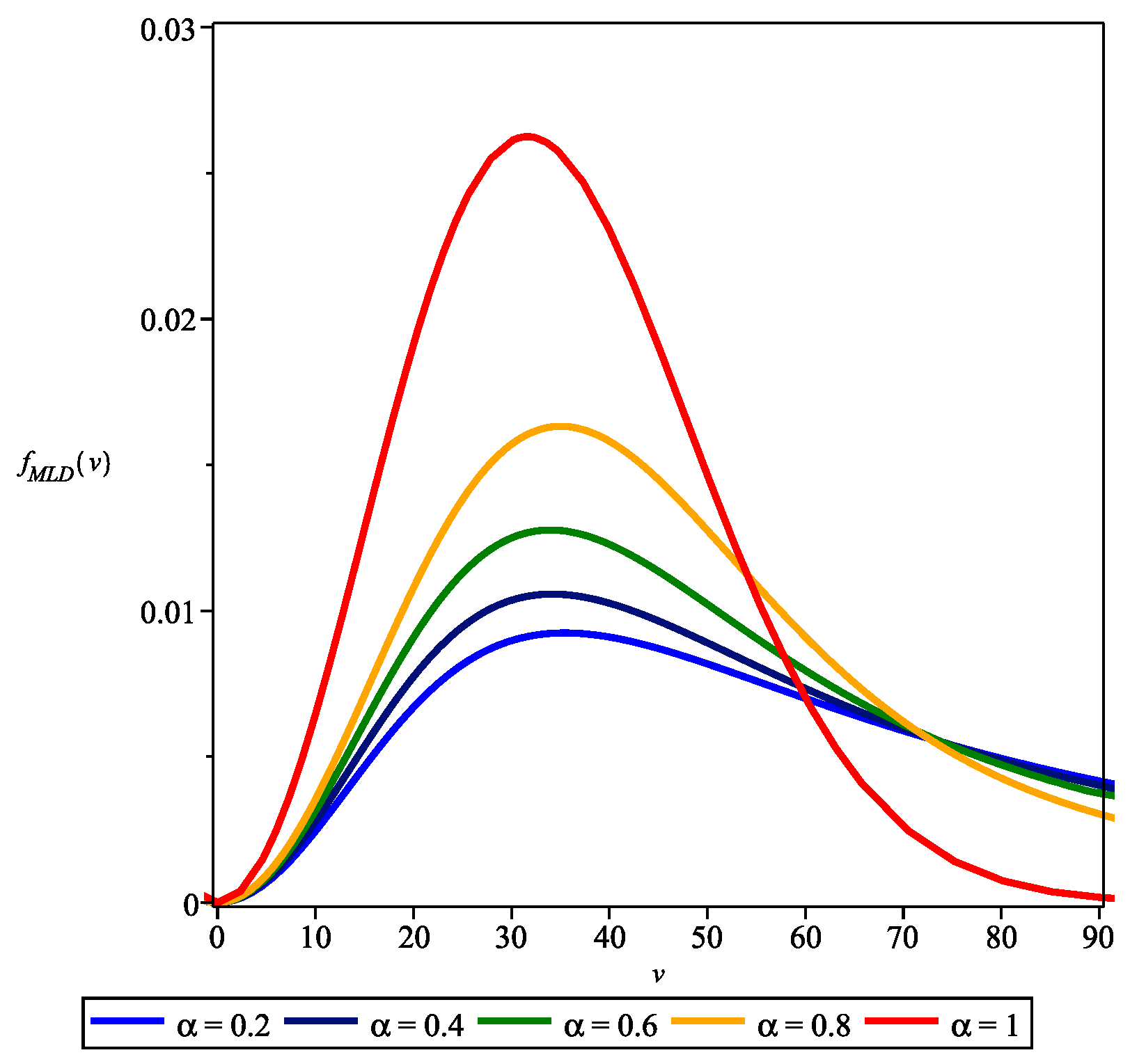
The figures below depict the velocity distribution in four different scenarios with a reduced mass of particles, μ = 1 . Figure 2 illustrates f M B D ( v ) for various values of T, while Figure 3 portrays the velocity distribution, f P D ( v ) , under various λ values, with T = 300 . Figure 4 and Figure 5 show the velocity distribution curves of the generalized Maxwell–Boltzmann case for T = 100 and T = 500 . It is readily seen that, when the parameter p is greater than 1, the distribution curve has heavy tails and shows that there is a higher probability of observing particles with very high energies. When p < 1 , the curve has lighter tail and can be applied to damped systems, while, for p = 1 , the curves coincide with classical Maxwell–Boltzmann cases, or stable cases, or equilibrium cases. Figure 6 displays the Mittag-Leffler velocity distribution of different α values, with T = 500 , and Figure 7 demonstrates the Mittag-Leffler velocity distribution of varying α values, with T = 700 . It can be observed that as the values of T increase in f M L ( v ) , the curve becomes heavy-tailed and less peaked in comparison to f P D ( v ) . Also, f M L ( v ) is less peaked when compared to f M B D ( v ) . It is evident from these observations that the Mittag-Leffler-modified velocity distribution f M L ( v ) is more general in nature and covers many classes of velocity distributions, including the Maxwell–Boltzmann velocity distribution f M B D ( v ) . From these figures, it is observable how the velocity distribution varies under non-perfect hydrostatic conditions, highlighting the differences captured by the Maxwell–Boltzmann distribution. Notably, the Maxwell–Boltzmann velocity distribution can be retrieved from the Mittag-Leffler-modified velocity distribution by setting α = 1 . It is worth noting that the Maxwell–Boltzmann velocity distribution also serves as a limiting case of the pathway velocity distribution.
The significance of altering the velocity distribution from the classical Maxwell–Boltzmann model is evident in several contexts. For instance, understanding the fusion reaction rates that contributed to the birth of our planet, which are the result of the Big Bang’s massive nuclear reactions, requires precise models. While the Maxwell–Boltzmann distribution provides a simplified theoretical framework, assuming stability and equilibrium, practically, conditions may not always align with these assumptions. Therefore, exploring alternative distributions becomes crucial. These alternatives allow for a more accurate representation of unstable or non-equilibrium processes, enhancing our ability to model and predict behaviors in complex systems. By adjusting the distribution function, we can better address the complexities of both stable and non-equilibrium scenarios. This study emphasizes the importance of altering the velocity distribution in a fusion plasma, transitioning from the conventional Maxwell–Boltzmann distribution to the pathway distribution and modified Mittag-Leffler distribution. This study has delved into the analysis of non-resonant modified thermonuclear functions under various scenarios, including classical Maxwell–Boltzmann and cut-off cases. These complex functions were elegantly expressed in closed forms, utilizing Fox’s H-function and incomplete H-functions, showcasing the versatility and applicability of these generalized special functions in high-energy physics. The graphs in the manuscript were plotted using Maple 2022.

Author Contributions

Writing—original draft, D.K. and A.A.K.; Writing—review & editing, H.J.H. All authors have read and agreed to the published version of the manuscript.

Funding

This research received no external funding.

Data Availability Statement

The original contributions presented in the study are included in the article, further inquiries can be directed to the corresponding author.

Acknowledgments

The authors would like to acknowledge the unknown referees for their valuable comments and suggestions, which enhanced the paper to its present form.

Conflicts of Interest

The authors declare no conflicts of interest.

Appendix A

This appendix addresses the evaluation techniques of the reaction rate integrals in non-relativistic cases. Consider a general integral of the form
T = 0 y ν 1 E α , α z y exp x y ρ d y ,
where z > 0 ,   x > 0 ,   ρ > 0 and 0 < α 1 . Taking the Mellin transform and using the definition of the gamma function, we obtain
M T ( s ) = 0 x s 1 0 y ν 1 E α , α z y exp x y ρ d y d x = Γ ( s ) 0 y ν + ρ s 1 E α , α z y d y = Γ ( s ) Γ ( ν + ρ s ) Γ ( 1 ν ρ s ) z ν + ρ s Γ ( α α ν α ρ s ) ,
where ( s ) > 0 , 0 < ( ν + ρ s ) < 1 . Using the inverse Mellin transform and Equation (A1), we obtain
T = 1 z ν H 1 , 3 2 , 1 ( z ρ x | ( ν , ρ ) ( 0 , 1 ) , ( ν , ρ ) , ( 1 α + α ν , α ρ ) ) .
Let us assume the reaction rate integral in the cut-off case to be
I ( x ) = 0 d y ν 1 E α , α z y exp x y ρ d y .
Let
f ( x 1 ) = x 1 ν E α , α z x 1 , if 0 x 1 < d < ,
and
g ( x 2 ) = exp x 2 ρ , if 0 x 2 < , ρ > 0 .
Using the Mellin convolution, we obtain
M I ( x ) ( s ) = M f ( s ) M g ( s ) ,
where
M f ( s ) = 0 d y ν + s 1 E α , α z y d y = k = 0 ( 1 ) k ( z d ) k Γ ( α k + α ) d ν + s Γ ( k + ν + s ) Γ ( k + ν + s + 1 ) ,
and
M g ( s ) = 0 y s 1 exp y ρ d y = 1 ρ Γ s ρ , ( s ) > 0 ,
Now, using (A5) and the inverse Mellin transform, we have
I x ρ = k = 0 ( 1 ) k ( z d ) k Γ ( α k + α ) d ν 2 π i ρ C Γ ( k + ν + s ) Γ s ρ Γ ( k + ν + s + 1 ) x d s d s ,
where C reperesents an appropriate contour. Using (1), we have
I ( x ) = d ν ρ k = 0 ( 1 ) k ( z d ) k Γ ( α k + α ) H 1 , 2 2 , 0 ( x 1 ρ d | ( k + ν + 1 , 1 ) ( k + ν , 1 ) , ( 0 , 1 ρ ) ) .
Also, one can represent the integral (A3) in terms of the incomplete H-function. Using the duplication formula on the gamma function, one can see from (A9) that I ( x ) in (A3) can also be represented in terms of Meijer’s G-function.

References

  1. Meijer, C. Über Whittakersche bezw. Besselsche Funktionen und deren Produkten. Nieuw Arch. Wisk. 1936, 18, 10–39. [Google Scholar]
  2. Fox, C. The G and H-functions as symmetrical Fourier kernels. Trans. Am. Math. Soc. 1961, 98, 395–429. [Google Scholar]
  3. Mathai, A.M.; Saxena, R.K.; Haubold, H.J. The H-Function: Theory and Applications; Springer: New York, NY, USA, 2010. [Google Scholar]
  4. Kilbas, A.A.; Saigo, M. On the H-function. J. Appl. Math. Stoch. Anal. 1999, 12, 191–204. [Google Scholar] [CrossRef]
  5. Kilbas, A.A.; Saigo, M. H-Transforms: Theory and Application; CRC Press: Boca Raton, FL, USA, 2004. [Google Scholar]
  6. Prudnikov, A.P.; Brychkov, Y.A.; Marichev, O.I. Integrals and Series; Gordon and Breach: New York, NY, USA, 1990; Volume 3. [Google Scholar]
  7. Buschman, R.G. H-function of two variables. Indian J. Math. 1978, 20, 105–116. [Google Scholar]
  8. Inayat-Hussain, A.A. New properties of hypergeometric series derivable from Feynman integrals: II. A generalization of the H-function. J. Phys. A Math. Gen. 1987, 20, 4119–4128. [Google Scholar] [CrossRef]
  9. Saxena, R.K.; Pogány, T.K. On fractional integration formulae for Aleph functions. Appl. Math. Comput. 2011, 218, 985–990. [Google Scholar] [CrossRef]
  10. Srivastava, H.M.; Saxena, R.K.; Parmar, R.K. Some Families of the Incomplete H-Functions and the Incomplete H ¯ -Functions and Associated Integral Transforms and Operators of Fractional Calculus with Applications. Russ. J. Math. Phys. 2018, 25, 116–138. [Google Scholar] [CrossRef]
  11. Shen, Y.P.; Guo, B.; Liu, W.P. Alpha-cluster transfer reactions: A tool for understanding stellar helium burning. Prog. Part. Nucl. Phys. 2021, 119, 103857. [Google Scholar] [CrossRef]
  12. Haubold, H.J.; Kumar, D. Extension of thermonuclear functions through the pathway model including Maxwell-Boltzmann and Tsallis’ distributions. Astropart. Phys. 2008, 29, 70–76. [Google Scholar] [CrossRef]
  13. Haubold, H.J.; Kabeer, A.A.; Kumar, D. Analytic forms of thermonuclear functions. Physica A 2023, 630, 129249. [Google Scholar] [CrossRef]
  14. Mathai, A.M. A pathway to matrix-variate gamma and normal densities. Linear Algebra Its Appl. 2005, 396, 317–328. [Google Scholar] [CrossRef]
  15. Tsallis, C. Possible generalization of Boltzmann–Gibbs statistics. J. Stat. Phys. 1998, 52, 479–487. [Google Scholar] [CrossRef]
  16. Agahi, H.; Alipour, M. Mittag-Leffler-Gaussian distribution: Theory and application to real data. Math. Comput. Simul. 2019, 156, 227–235. [Google Scholar] [CrossRef]
  17. Gorenflo, R.; Kilbas, A.A.; Mainardi, F.; Rogosin, S.V. Mittag-Leffler Functions, Related Topics and Applications, 2nd ed.; Springer Monographs in Mathematics; Springer: Berlin, Germany, 2020. [Google Scholar]
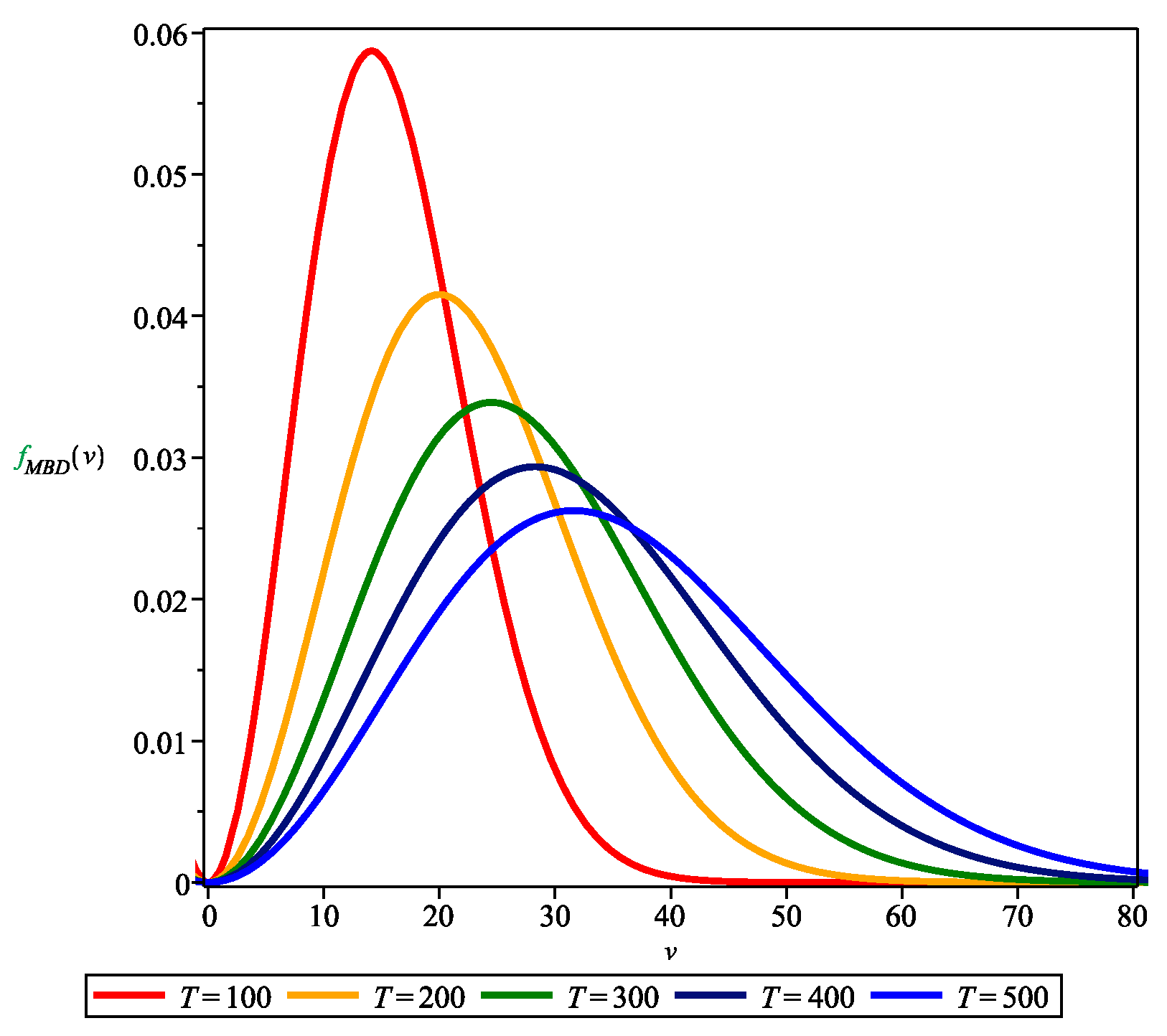
Figure 2. f M B D ( v ) for T = 100 , 200 , 300 , 400 , 500 .
Axioms 13 00532 g002
Figure 3. f P D ( v ) for T = 300 and β = 1.1 , 1.2 , 1.3 , 1.4 , 1.5 .
Axioms 13 00532 g003
Figure 4. f G M B ( v ) for T = 100 and p = 1.0 , 1.1 , 1.2 , 1.3 , 1.4 .
Axioms 13 00532 g004
Figure 5. f G M B ( v ) for T = 500 and p = 1.0 , 1.1 , 1.2 , 1.3 , 1.4 .
Axioms 13 00532 g005
Figure 6. f M L ( v ) for T = 500 and α = 0.2 , 0.4 , 0.6 , 0.8 , 1 .
Axioms 13 00532 g006
Figure 7. f M L ( v ) for T = 700 and α = 0.2 , 0.4 , 0.6 , 0.8 , 1 .
Axioms 13 00532 g007
Disclaimer/Publisher’s Note: The statements, opinions and data contained in all publications are solely those of the individual author(s) and contributor(s) and not of MDPI and/or the editor(s). MDPI and/or the editor(s) disclaim responsibility for any injury to people or property resulting from any ideas, methods, instructions or products referred to in the content.