On Lebesgue Constants

Abstract

Simple formulae for Lebesgue constants arising in the classical Fourier series approximation are obtained. Both even and odd cases are addressed, extending Fejér’s results. Asymptotic formulae are also obtained.

1. Introduction

There are many famous important constants in mathematics, such as e (Napier’s constant or Euler’s number), $\pi$ (Archimedes’ constant), $\sqrt{2}$ (Pythagoras’ constant), and $\gamma$ (Euler’s constant), to cite a few [1]. In this article, we will deal with the Lebesgue constants that were introduced by H. Lebesgue as the best possible upper bound for the approximation of functions through Fourier series [2,3,4]. These numbers are usually expressed in the form

$$I_n={\displaystyle \frac{1}{\pi }}{\int }_0^{\pi }{\displaystyle \frac{|sin((n+1/2)t\left)\right|}{sin(t/2)}}dt$$

(1)

where $n\in \mathbb{N}.$

Several famous mathematicians have worked on these constants and established some properties, such as asymptotic and proposed alternative expressions. Here are some of them.

• Fejér [5] proved the formula

  $$I_n={\displaystyle \frac{1}{2n+1}}+{\displaystyle \frac{2}{\pi }}\sum _{k=1}^n{\displaystyle \frac{1}{k}}tan\left({\displaystyle \frac{k\pi }{2n+1}}\right),n\in \mathbb{N};$$

  (2)
• Szegö [6] contributed with the formula

  $$I_n={\displaystyle \frac{16}{{\pi }^2}}\sum _{k=1}^{\infty }\sum _{j=1}^{(2n+1)k}{\displaystyle \frac{1}{4k^2-1}}{\displaystyle \frac{1}{2j-1}},n\in \mathbb{N};$$

  (3)
• Watson [7] established the following asymptotic expression:

  $$\underset{n\to \infty }{lim}\left(I_n-{\displaystyle \frac{4}{{\pi }^2}}ln\left(2n+1\right)\right)=c$$

  (4)

  where

  $$c={\displaystyle \frac{8}{{\pi }^2}}\sum _{k=1}^{\infty }{\displaystyle \frac{ln\left(k\right)}{4k^2-1}}-{\displaystyle \frac{4}{{\pi }^2}}\psi \left({\displaystyle \frac{1}{2}}\right)={\displaystyle \frac{4}{{\pi }^2}}(2.4413238136\dots ),$$

  (5)

  and $\psi \left(x\right)$ is the digamma function;
• Hardy [8] discovered two integral representations

  $$\begin{array}{cc}\hfill I_n& =4\underset{0}{\overset{\infty }{\int }}{\displaystyle \frac{tanh\left((2n+1)x\right)}{tanh\left(x\right)}}{\displaystyle \frac{1}{\pi 2+4x^2}}dx\hfill \\ \hfill & =\underset{0}{\overset{\infty }{\int }}{\displaystyle \frac{sinh\left((2n+1)x\right)}{sinh\left(x\right)}}ln\left(coth\left({\displaystyle \frac{2n+1}{2}}x\right)\right)dx.\hfill \end{array}$$

  (6)

  Later, other mathematicians contributed with two-sided estimates. Zhao [9] discovered bilateral inequalities that help improve Watson’s asymptotic expansion formulae. In [3], new inequalities for the Lebesgue constants $I_{n/2}$ were established, which allowed the authors to obtain an asymptotic expansion of $I_{n/2}$ in terms of ${\displaystyle \frac{1}{n+1}}$. More recently, other contributions have been published. Shakirov approximated the Lebesgue constant using a logarithmic function [10] and using the logarithmic–fractional–rational function [4]. The asymptotic behavior of $I_n$ was also studied in [11], although indirectly, since the authors studied the properties of the Dirichlet kernel, which is related to the integrand function appearing in (8). It must be remarked that (1) can be rewritten in the form

  $$I_n={\displaystyle \frac{2}{\pi }}{\int }_0^{\pi /2}{\displaystyle \frac{|sin((2n+1)t\left)\right|}{sin\left(t\right)}}dt$$

  (7)

  where $n\in \mathbb{N}.$ As $2n+1,n\in \mathbb{N},$ is an odd integer, we are interested in treating the even case too. Therefore, the main goals of the paper are as follows:

• Consider the more general expression

  $$I_n={\displaystyle \frac{2}{\pi }}{\int }_0^{\pi /2}{\displaystyle \frac{|sin(nt\left)\right|}{sin\left(t\right)}}dt,n\in \mathbb{N},$$

  (8)

  keeping the designation “Lebesgue constants”;
• Reproduce Fejér’s results using a simpler approach;
• Obtain simple asymptotic formulae.

Below, we describe the steps involved in obtaining Fejér’s formula for Lebesgue numbers of any integer order. The main idea is expressed in the decomposition of the function $\left|sin\right(nt\left)\right|$ into a finite, well-defined, sum of copies of the same “bump” function (Section 3.1). Then, all that is needed is to integrate such a finite sum and simplify the resulting expression. We consider, separately, the even case ($n=2N$), obtaining a new formula stated in (15), and the odd case ($n=2N+1$), where we reobtain Fejér’s formula (23). Finally, asymptotic formulae are proposed. For them, we study the odd-order case first and deduce the even case from it. The asymptotic properties of the Dirichlet kernel are used [12].

The manuscript is structured as follows. Section 2 contains some important results that will help us find exact closed formulae for (8). In particular, we express the Dirichlet kernel as a finite trigonometric sum. In Section 3, we deduce the formulae that extend the Fejér result. Finally, the asymptotic formulae are studied in Section 4.

2. The Way to the Lebesgue Constants

Lebesgue studied the approximation of periodic functions by means of the partial sum of the Fourier series [2] and obtained a formulation that can be stated as follows [11].

Theorem 1. 

Let $f\left(t\right)$ be a periodic continuous function on $[-\pi ,\pi ],$ and

$$C_k={\displaystyle \frac{1}{2\pi }}{\int }_{-\pi }^{\pi }f\left(t\right)e^{-ikt}dt,$$

The Fourier coefficients, where $i=\sqrt{-1}$. If $S_n\left(f\right),n\in \mathbb{N},$ denote the $n^{\mathrm{th}}$ partial sum of $f\left(t\right)$, that is,

$$S_n\left(f\right)=\sum _{k=-n}^n{C}_k{e}^{ikt},$$

(9)

Then,

$$S_n\left(f\right)={\displaystyle \frac{1}{2\pi }}{\int }_{-\pi }^{\pi }{D}_n\left(\tau \right)f(t-\tau )d\tau ,$$

(10)

where

$$D_n\left(t\right)=\left\{\begin{array}{cc}{\displaystyle \frac{sin\left(\right(n+1/2\left)t\right)}{sin(t/2)}}\hfill & t\ne 0\hfill \\ 2n+1\hfill & t=0\hfill \end{array}\right.$$

(11)

is the so-called Dirichlet kernel.

This theorem shows the importance of the Dirichlet kernel and the relation with the Lebesgue constants. Lebesgue showed the following.

Corollary 1. 

If

$$\underset{-\pi \le t\le \pi }{max}\left|f\left(t\right)\right|\le 1,$$

then

$$\underset{-\pi \le t\le \pi }{max}|S_n\left(f\right)|\le {\displaystyle \frac{1}{2\pi }}{\int }_{-\pi }^{\pi }\left|D_n\left(t\right)\right|dt,$$

(12)

where ${\displaystyle \frac{1}{2\pi }}{\int }_{-\pi }^{\pi }\left|D_n\left(t\right)\right|dt$ is the best possible upper bound.

The Dirichlet kernel verifies the following relation [11]:

$$4+{\displaystyle \frac{8}{\pi }}ln\left(n+{\displaystyle \frac{1}{2}}\right)\le {\int }_{-\pi }^{\pi }\left|{\mathcal{D}}_n\left(t\right)\right|dt\le 2\pi +4+{\displaystyle \frac{8}{\pi }}ln\left(2n\right),$$

which can be used to find the asymptotic behavior of the Lebesgue constants. As referred above, we consider the general expression stated in (8).

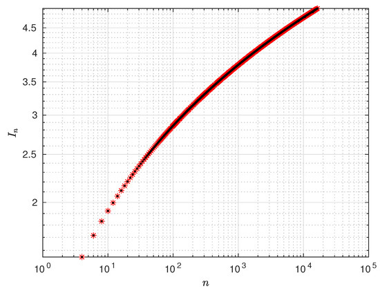
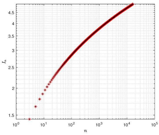
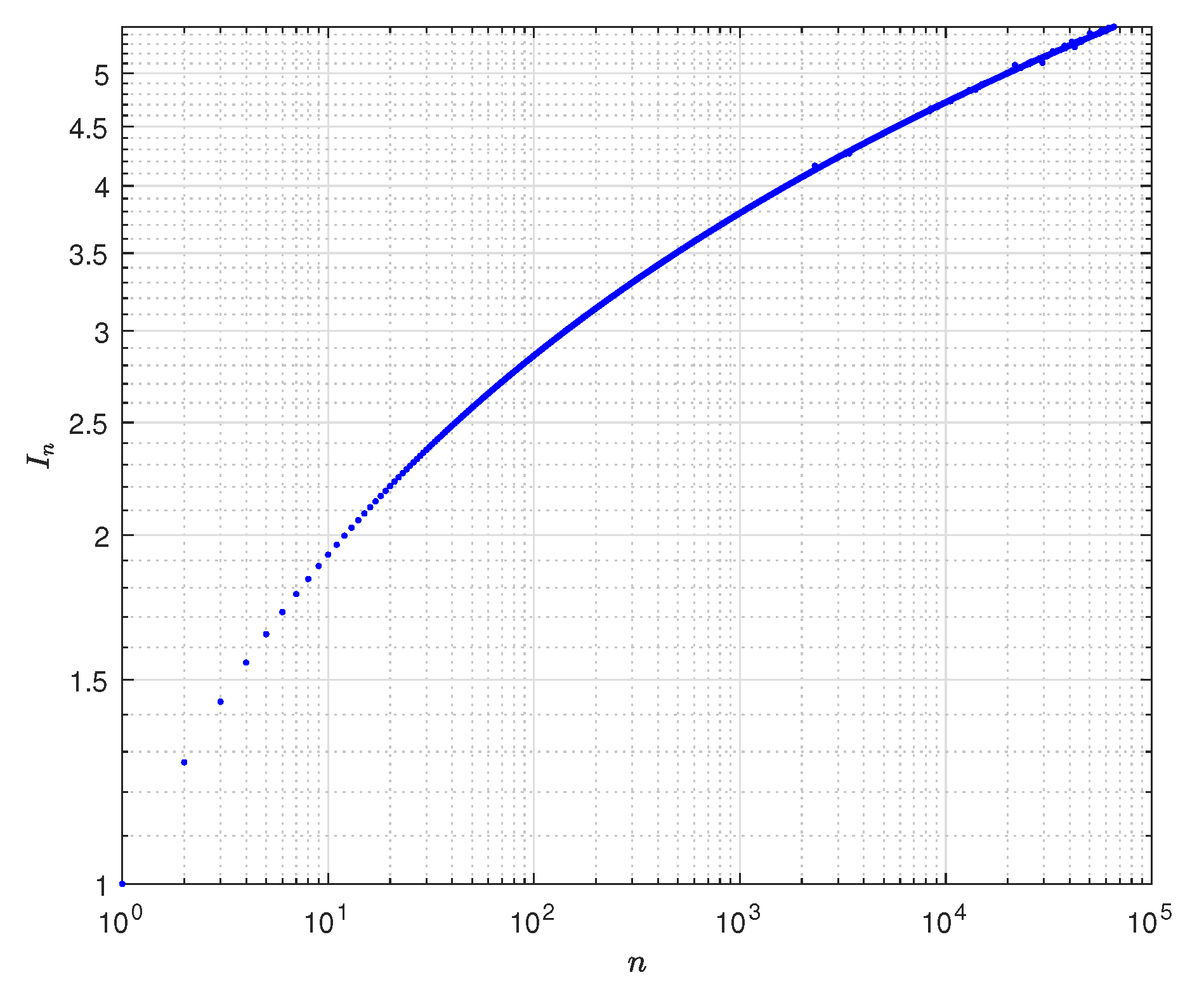
We propose an alternative approach that leads to exact closed formulae corresponding to any positive value of $n\in \mathbb{N}$. In the following picture (see Figure 1), we show the result of the numerical integration of (8) for $n=1,2,3,\cdots 2^L$, with $L=16$. We used a log-scale.

Figure 1. Examples for $n=1,2,\cdots$.

We continue by establishing a result that will be useful in a later section. Let us define the Dirichlet-like kernel given by

$${\overline{D}}_n\left(t\right)={\displaystyle \frac{sin\left(nt\right)}{sin\left(t\right)}}$$

Theorem 2. 

The Dirichlet-like kernel can be expressed as

$${\overline{D}}_n\left(t\right)={\displaystyle \frac{sin\left(nt\right)}{sin\left(t\right)}}=e^{i(n-1)t}+e^{i(n-3)t}+\cdots +e^{-i(n-3)t}+e^{-i(n-1)t}$$

(13)

Proof. 

The proof is immediate. We only need to note that

$${\displaystyle \frac{sin\left(nt\right)}{sin\left(t\right)}}={\displaystyle \frac{e^{int}-e^{-int}}{e^{it}-e^{-it}}}=e^{i(n-1)t}{\displaystyle \frac{1-e^{-i2nt}}{1-e^{-i2t}}}$$

and apply the geometric sum rule. □

The exponents in (13) have the generic form $i(n-(2k-1\left)\right)t,k=1,2,\cdots$. Only if n is odd can it assume the value 0. This results in the following consequence.

Corollary 2. 

Let

$$N=\left\{\begin{array}{cc}{\displaystyle \frac{n-1}{2}},\hfill & \mathit{if}n\mathit{is}\mathit{odd}\hfill \\ {\displaystyle \frac{n}{2}},\hfill & \mathit{if}n\mathit{is}\mathit{even}\hfill \end{array}\right..$$

Then,

$${\overline{D}}_n\left(t\right)={\displaystyle \frac{sin\left(nt\right)}{sin\left(t\right)}}=\left\{\begin{array}{cc}1+2\sum _{k=1}^{N}cos\left(2kt\right)\hfill & \mathit{if}n\mathit{is}\mathit{odd}\hfill \\ 2\sum _{k=1}^{N}cos\left((2k-1)t\right)\hfill & \mathit{if}n\mathit{is}\mathit{even}\hfill \end{array}\right..$$

(14)

This expression is suitable for obtaining the primitive of ${\overline{D}}_n\left(t\right).$

3. New Formulation

3.1. Preliminaries

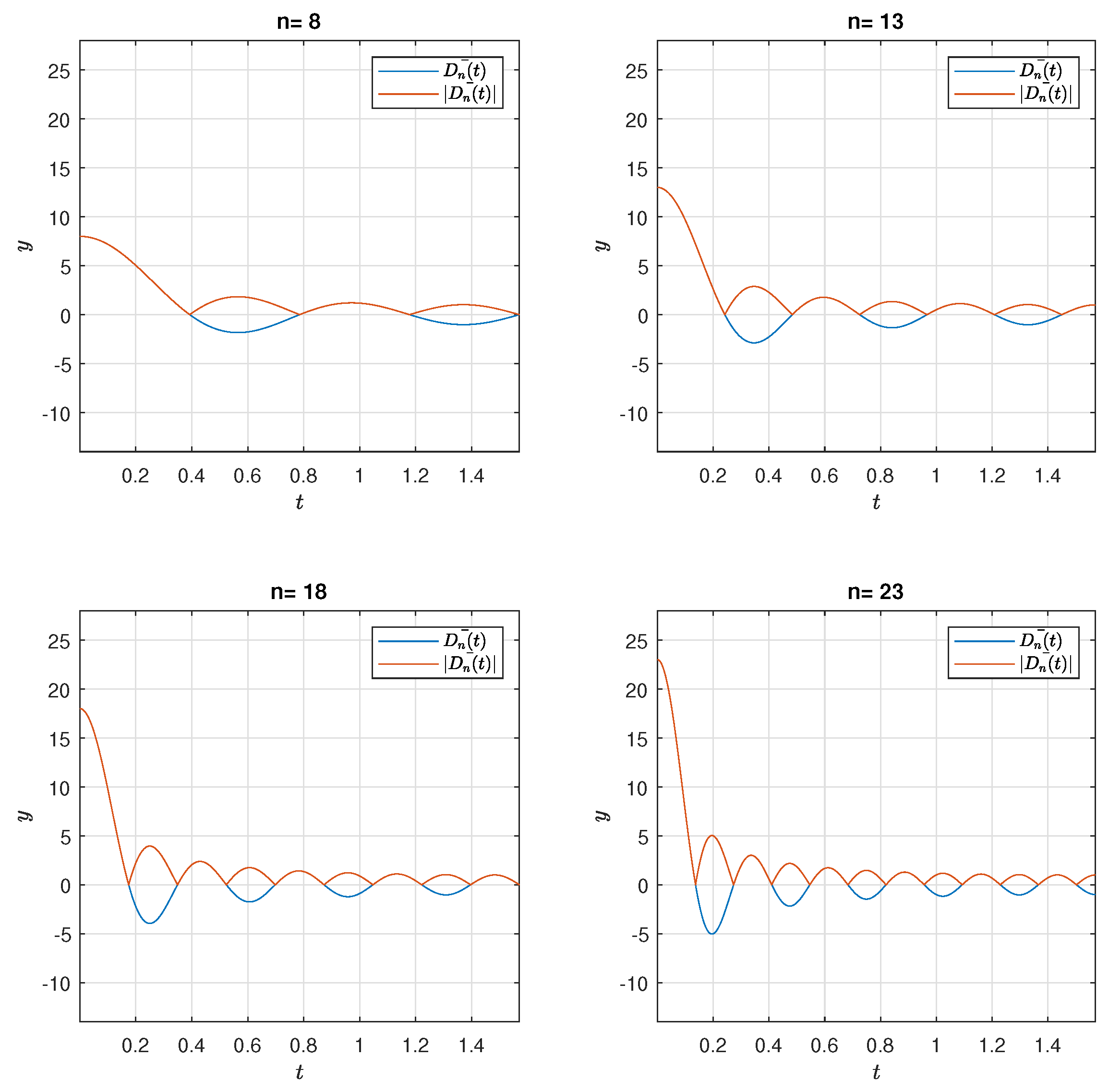
Let us conduct a brief study of the kernel that will help us find the solution we are looking for. Consider the function

$$f\left(t\right)=|sin(nt\left)\right|,0\le t\le \pi /2,$$

where the sinusoid $sin\left(nt\right)$ has the frequency ${\displaystyle \frac{n}{2\pi }}$ and half-period $T={\displaystyle \frac{\pi }{n}}$. Therefore, in the interval $0\le t\le \pi /2$, there are N half periods. If n is odd, there is another quarter period. In the half periods with orders $0,2,4,\cdots$ the function $sin\left(nt\right)$ is positive. In the others, it is negative (see Figure 2).

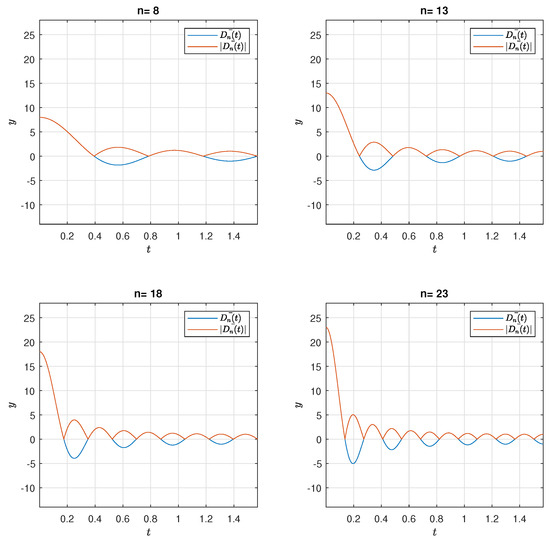
Figure 2. Representations of ${\overline{D}}_n\left(t\right)$ and $|{\overline{D}}_n\left(t\right)|$ for $n=8,13,18,23.$.

Therefore, the presence of the absolute value in $f\left(t\right)$ allows us to write

$$f\left(t\right)=\sum _{m=0}^N{f}_m\left(t\right),$$

where

$$f_m\left(t\right)=f_{m-1}(t-T),mT\le t<(m+1)T,m=1,2,\cdots N-1,$$

with $f_0\left(t\right)=sin\left(nt\right),0\le t<T,$ and the last term $(m=N)$.

$$f_N\left(t\right)=\left\{\begin{array}{cc}{f}_{N-1}(t-T),NT\le t<NT+T/2,\hfill & \mathit{if}N\mathit{is}\mathit{odd}\hfill \\ 0,\hfill & \mathit{if}N\mathit{is}\mathit{even}\hfill \end{array}\right..$$

This means that $f\left(t\right)$ is obtained by juxtaposing N positive half periods of $sin\left(nt\right)$. If n is odd, we have to join another one quarter of a period.

3.2. The Even n Case

Theorem 3. 

Let $n\in \mathbb{N}$ be an even number. Then,

$$I_n={\displaystyle \frac{4}{\pi }}\sum _{k=1}^{n/2}{\displaystyle \frac{tan\left(\frac{(2k-1)\pi }{2n}\right)}{2k-1}}.$$

(15)

Proof. 

According to the structure of the numerator of our kernel, we can write

$$I_n={\displaystyle \frac{2}{\pi }}\sum _{m=0}^{N-1}{\int }_{mT}^{(m+1)T}{\displaystyle \frac{sin\left(n\right(t-mT\left)\right)}{sin\left(t\right)}}dt$$

(16)

Attending to

$$sin\left(nt\right)=sin\left(n(t+mT-mT)\right)=sin(n(t+mT)-m\pi )={(-1)}^{m}sin\left(n(t+mT)\right),$$

(17)

we are led to

$$I_n={\displaystyle \frac{2}{\pi }}\sum _{m=0}^{N-1}{(-1)}^m\left[{\int }_0^T{\displaystyle \frac{sin\left(n\right(t+mT\left)\right)}{sin(t+mT)}}dt\right],$$

(18)

which expresses the Lebesgue numbers in a new different way.

To continue, we need to find the primitive of the integrand, which is not a big task. In fact, as we saw above,

$${\displaystyle {\displaystyle \frac{sin\left(nx\right)}{sin\left(x\right)}}=2\sum _{k=1}^{N}cos\left((2k-1)x\right).}$$

It follows that

$${\displaystyle P_n\left(x\right)=\int {\displaystyle \frac{sin\left(nx\right)}{sinx}}dx=2\sum _{k=1}^N{\displaystyle \frac{sin\left(\right(2k-1\left)x\right)}{2k-1}}.}$$

(19)

For our application, $x=t+mT$, so that

$${\displaystyle P_n\left(t\right)=\int {\displaystyle \frac{sin\left(n\right(t+mT\left)\right)}{sin(t+mT)}}dt=2\sum _{k=1}^{n/2}{\displaystyle \frac{sin\left(\right(2k-1\left)\right(t+mT\left)\right)}{2k-1}}.}$$

(20)

Let us denote the function in brackets in (18) by $J_m\left(n\right)$. We have

$$I_n={\displaystyle \frac{2}{\pi }}\sum _{m=0}^{N-1}{(-1)}^m{J}_m\left(n\right).$$

(21)

with

$$J_m\left(n\right)={\int }_0^T{\displaystyle \frac{sin\left(n\right(t+mT\left)\right)}{sin(t+mT)}}dt=P_n\left(T\right)-P_n\left(0\right),$$

where $T=\pi /n$. Then, $mT={\displaystyle \frac{\pi m}{n}}$, $T+mT={\displaystyle \frac{(m+1)\pi }{n}}$, and

$${\displaystyle J_m\left(n\right)=2\sum _{k=1}^N{\displaystyle \frac{sin\left(\right(2k-1\left)\right(m+1)\pi /n)}{2k-1}}-2\sum _{k=1}^N{\displaystyle \frac{sin\left(\right(2k-1)m\pi /n)}{2k-1}}.}$$

Simplifying

$${\displaystyle J_m\left(n\right)=2\sum _{k=1}^N{\displaystyle \frac{sin\left(\right(2k-1\left)\right(m+1)\pi /n)-sin\left(\right(2k-1)m\pi /n)}{2k-1}},}$$

and using the trigonometric identity $sin\left(A\right)-sin\left(B\right)=2cos\left({\displaystyle \frac{A+B}{2}}\right)sin\left({\displaystyle \frac{A-B}{2}}\right),$ we obtain

$${\displaystyle J_m\left(n\right)=4\sum _{k=1}^N{\displaystyle \frac{cos\left(\right(2k-1\left)\right(2m+1)\pi /(2n\left)\right)sin\left(\right(2k-1)\pi /(2n\left)\right)}{2k-1}}.}$$

(22)

That inserted into (21) gives the expected result. However, we can manipulate these formulae in an attempt to achieve any simplification. We proceed to reverse the summation order:

$$\begin{array}{cc}\hfill \sum _{m=0}^{N-1}{(-1)}^m& \left(\sum _{k=1}^N{\displaystyle \frac{cos\left(\right(2k-1\left)\right(2m+1)\pi /(2n\left)\right)sin\left(\right(2k-1)\pi /(2n\left)\right)}{2k-1}}\right)=\hfill \\ & \sum _{k=1}^N{\displaystyle \frac{sin\left(\right(2k-1)\pi /(2n\left)\right)}{2k-1}}\left(\sum _{m=0}^{N-1}{(-1)}^{m}cos\left((2k-1)(2m+1)\pi /\left(2n\right)\right)\right)\hfill \end{array}$$

By replacing a sinusoid with exponentials and using the sum rule of the geometric sequence, we can show that

$$\sum _{m=0}^{N-1}{(-1)}^{m}cos\left((2k-1)(2m+1)\pi /\left(2n\right)\right)={\displaystyle \frac{1-{(-1)}^{N}cos\left(\frac{N}{n}(2k-1)\pi \right)}{2cos\left({\displaystyle \frac{(2k-1)\pi }{2n}}\right)}}$$

Attending to the fact that $2N=n$ and $cos\left((2k-1)\pi /2\right)=0$, we can write

$$\sum _{m=0}^{N-1}{(-1)}^{m}cos\left((2k-1)(2m+1)\pi /n\right)={\displaystyle \frac{1}{2cos\left({\displaystyle \frac{(2k-1)\pi }{2n}}\right)}}$$

and, finally, (15). □

This formula was never proposed. In Figure 3, we compare the value of $I_n$ obtained from (15) with the numerical integration of (8).

Figure 3. Comparison of (15) (red) with numerical integration of (8) (black).

3.3. The Odd n Case

Theorem 4. 

Let $n\in \mathbb{N}$ be an odd number. Then,

$$I_n={\displaystyle \frac{2}{\pi }}\sum _{k=1}^{(n-1)/2}{\displaystyle \frac{tan(k\pi /n)}{k}}+{\displaystyle \frac{1}{n}}$$

(23)

This formula was proposed first by Fejér but deduced using a completely different procedure [5].

Proof. 

Let $n=2N+1$. Unlike the even n case, we have

$$I_n={\displaystyle \frac{2}{\pi }}\sum _{m=0}^{N-1}{\int }_{mT}^{(m+1)T}{\displaystyle \frac{sin\left(n\right(t-mT\left)\right)}{sin\left(t\right)}}dt+{\displaystyle \frac{2}{\pi }}{\int }_{NT}^{NT+T/2}{\displaystyle \frac{sin\left(n\right(t-NT\left)\right)}{sin\left(t\right)}}dt.$$

(24)

We joined an extra quarter of a period.

Using (17), the second term on the right of the equality is

$${\int }_{NT}^{NT+T/2}{\displaystyle \frac{sin\left(n\right(t-NT\left)\right)}{sin\left(t\right)}}dt={\int }_0^{T/2}{\displaystyle \frac{sin\left(nt\right)}{sin(t+NT)}}dt={\int }_0^{T/2}{\displaystyle \frac{{(-1)}^{N}sin\left(n(t+NT)\right)}{sin(t+NT)}}dt$$

and

$$I_n={\displaystyle \frac{2}{\pi }}\left[\sum _{m=0}^{N-1}{(-1)}^m{\int }_0^T{\displaystyle \frac{sin\left(n\right(t+mT\left)\right)}{sin(t+mT)}}dt+{\int }_0^{T/2}{(-1)}^N{\displaystyle \frac{sin\left(n\right(t+NT\left)\right)}{sin(t+NT)}}dt\right],$$

(25)

which re-expresses the Lebesgue numbers in a new, different way.

To continue, we need to find the primitive of the integrand, which is not a big task given (14). In fact, we have

$${\displaystyle {\displaystyle \frac{sin\left(nx\right)}{sin\left(x\right)}}=1+2\sum _{k=1}^{(n-1)/2}cos2kx,}$$

It follows that

$${\displaystyle P_n\left(x\right)=\int {\displaystyle \frac{sin\left(nx\right)}{sinx}}dx=\sum _{k=1}^{(n-1)/2}{\displaystyle \frac{sin2kx}{k}}+x.}$$

For our application, $x=t+mT$, so that

$${\displaystyle P_n\left(t\right)=\int {\displaystyle \frac{sin\left(n\right(t+mT\left)\right)}{sin(t+mT)}}dt=\sum _{k=1}^N{\displaystyle \frac{sin\left(2k(t+mT)\right)}{k}}+(t+mT).}$$

(26)

As above, let us denote the function in brackets in (25) by $J_m\left(n\right)$ and the second term by $J_N\left(n\right)$ so that

$$I_n={\displaystyle \frac{2}{\pi }}\sum _{m=0}^{N-1}{(-1)}^m{J}_m\left(n\right)+{\displaystyle \frac{2}{\pi }}{J}_N\left(n\right)$$

(27)

with

$$J_m\left(n\right)={\int }_0^T{\displaystyle \frac{sin\left(n\right(t+mT\left)\right)}{sin(t+mT)}}dt=P_n\left(T\right)-P_n\left(0\right),$$

and

$$J_N\left(n\right)={\int }_0^{T/2}{\displaystyle \frac{sin\left(n\right(t+mT\left)\right)}{sin(t+mT)}}dt=P_n(T/2)-P_n\left(0\right).$$

As $T=\pi /n$, then $mT={\displaystyle \frac{\pi m}{n}}$, $T+mT={\displaystyle \frac{(m+1)\pi }{n}}$, and

$${\displaystyle J_m\left(n\right)=\sum _{k=1}^N{\displaystyle \frac{sin\left(2k(m+1)\pi /n\right)}{k}}+{\displaystyle \frac{(m+1)\pi }{n}}-\sum _{k=1}^N{\displaystyle \frac{sin(2km\pi /n)}{k}}+{\displaystyle \frac{m\pi }{n}}.}$$

We obtain

$${\displaystyle J_m\left(n\right)=\sum _{k=1}^N{\displaystyle \frac{sin\left(2k(m+1)\pi /n\right)-sin(2km\pi /n)}{k}}+{\displaystyle \frac{\pi }{n}}.}$$

Using the trigonometric identity $sin\left(A\right)-sin\left(B\right)=2cos\left({\displaystyle \frac{A+B}{2}}\right)sin\left({\displaystyle \frac{A-B}{2}}\right),$

$${\displaystyle J_m\left(n\right)=2\sum _{k=1}^N{\displaystyle \frac{cos\left(k(2m+1)\pi /n\right)sin(k\pi /n)}{k}}+{\displaystyle \frac{\pi }{n}}.}$$

(28)

Concerning the other term, $J_N\left(n\right)$, we have

$${\displaystyle J_N\left(n\right)=\sum _{k=1}^N{\displaystyle \frac{sin\left(2k(T/2+NT)\right)}{k}}+(T/2+NT)-\sum _{k=1}^N{\displaystyle \frac{sin(2kN\pi /n)}{k}}-NT.}$$

But $n=2N+1$ and $Tn=\pi$, allowing a simplification of the above expression:

$${\displaystyle J_N\left(n\right)=\sum _{k=1}^N{(-1)}^k{\displaystyle \frac{sin(k\pi /n)}{k}}+{\displaystyle \frac{\pi }{2n}}.}$$

(29)

Let us manipulate these formulae trying to achieve simplifications. We turn our attention to (27)–(29). Then,

$$\begin{array}{cc}\hfill I_n={\displaystyle \frac{4}{\pi }}& \sum _{m=0}^{N-1}{(-1)}^m\left({\displaystyle \sum _{k=1}^N{\displaystyle \frac{cos\left(k(2m+1)\pi /n\right)sin(k\pi /n)}{k}}}\right)+\hfill \\ & {\displaystyle {\displaystyle \frac{2}{\pi }}{(-1)}^N\sum _{k=1}^N{(-1)}^k{\displaystyle \frac{sin(k\pi /n)}{k}}+{\displaystyle \frac{2}{n}}\sum _{m=0}^{N-1}{(-1)}^m+{(-1)}^N{\displaystyle \frac{1}{n}},}\hfill \end{array}$$

or

$$\begin{array}{cc}\hfill I_n={\displaystyle \frac{4}{\pi }}& \sum _{m=0}^{N-1}{(-1)}^m\left({\displaystyle \sum _{k=1}^N{\displaystyle \frac{cos\left(k(2m+1)\pi /n\right)sin(k\pi /n)}{k}}}\right)+\hfill \\ & {\displaystyle {\displaystyle \frac{2}{\pi }}{(-1)}^N\sum _{k=1}^N{(-1)}^k{\displaystyle \frac{sin(k\pi /n)}{k}}+{\displaystyle \frac{1}{n}}.}\hfill \end{array}$$

(30)

Let us change the summation order in the first term on the right in expression (30):

$$\begin{array}{cc}\hfill \sum _{m=0}^{N-1}{(-1)}^m& \left(\sum _{k=1}^N{\displaystyle \frac{cos\left(k(2m+1)\pi /n\right)sin(k\pi /n)}{k}}\right)=\hfill \\ \hfill & \sum _{k=1}^N{\displaystyle \frac{sin(k\pi /n)}{k}}\left(\sum _{m=0}^{N-1}{(-1)}^{m}cos\left(k(2m+1)\pi /n\right)\right).\hfill \end{array}$$

Observe that

$$\sum _{m=0}^{N-1}{(-1)}^{m}cos\left(k(2m+1)\pi /n\right)={\displaystyle \frac{1-{(-1)}^{N}cos\left({\displaystyle \frac{2N}{n}}k\pi \right)}{2cos\left(k{\displaystyle \frac{\pi }{n}}\right)}}.$$

(31)

But, $2N=n-1$, so that

$$cos\left({\displaystyle \frac{2N}{n}}k\pi \right)=cos\left(\left(1-{\displaystyle \frac{1}{n}}\right)k\pi \right)={(-1)}^{k}cos\left(k{\displaystyle \frac{\pi }{n}}\right).$$

Hence,

$$\sum _{m=0}^{N-1}{(-1)}^{m}cos\left(k(2m+1)\pi /n\right)={\displaystyle \frac{1-{(-1)}^{N+k}cos\left(k{\displaystyle \frac{\pi }{n}}\right)}{2cos\left(k{\displaystyle \frac{\pi }{n}}\right)}}={\displaystyle \frac{1}{2cos\left(k{\displaystyle \frac{\pi }{n}}\right)}}-{(-1)}^{N+k}{\displaystyle \frac{1}{2}},$$

which leads to

$$\begin{array}{cc}\hfill \sum _{m=0}^{N-1}{(-1)}^m& \left(\sum _{k=1}^N{\displaystyle \frac{cos\left(k(2m+1)\pi /n\right)sin(k\pi /n)}{k}}\right)=\hfill \\ & {\displaystyle \frac{1}{2}}\sum _{k=1}^N{\displaystyle \frac{sin(k\pi /n)}{k}}\left({\displaystyle \frac{1}{cos\left(k\pi /n\right)}}-{(-1)}^{N+k}\right)=\hfill \\ & {\displaystyle \frac{1}{2}}\sum _{k=1}^N{\displaystyle \frac{tan(k\pi /n)}{k}}-{\displaystyle \frac{{(-1)}^N}{2}}\sum _{k=1}^N{(-1)}^k{\displaystyle \frac{sin(k\pi /n)}{k}}.\hfill \end{array}$$

Inserting it into (30), we obtain

$$\begin{array}{cc}\hfill I_n={\displaystyle \frac{2}{\pi }}& \sum _{k=1}^N{\displaystyle \frac{tan(k\pi /n)}{k}}-{\displaystyle \frac{2}{\pi }}{(-1)}^N\sum _{k=1}^N{(-1)}^k{\displaystyle \frac{sin(k\pi /n)}{k}}+\hfill \\ & {\displaystyle {\displaystyle \frac{2}{\pi }}{(-1)}^N\sum _{k=1}^N{(-1)}^k{\displaystyle \frac{sin(k\pi /n)}{k}}+{\displaystyle \frac{1}{n}}.}\hfill \end{array}$$

(32)

Finally, we obtain (23). □

In Figure 4, we compare (23) with the integral representation of $I_n$ (8).

Figure 4. Comparison of (23) (red) with (8) (black).

To make a comparison of the two situations, let us return and rewrite the two expressions for $I_n$, for $n=2N$ and $n=2N+1$, with $1<N\in \mathbb{N}.$ For each N, we obtain

$$\begin{array}{cc}\hfill I_{2N}& ={\displaystyle \frac{4}{\pi }}\sum _{k=1}^N{\displaystyle \frac{tan\left(\frac{(2k-1)\pi }{2n}\right)}{2k-1}}\hfill \\ \hfill I_{2N+1}& ={\displaystyle \frac{4}{\pi }}\sum _{k=1}^N{\displaystyle \frac{tan\left(\frac{2k\pi }{2n}\right)}{2k}}+{\displaystyle \frac{1}{2N+1}}.\hfill \end{array}$$

(33)

It is interesting to remark the important fact that the first summation involves odd samples of the function ${\displaystyle \frac{tan\left(\pi x\right)}{x}}$, while the second involves even samples.

4. Asymptotic Behavior

Let us consider the odd n case first and turn our attention to (27):

$$\begin{array}{cc}\hfill I_n={\displaystyle \frac{2}{\pi }}\sum _{m=0}^{N-1}{(-1)}^m& \left[{\displaystyle \sum _{k=1}^N{\displaystyle \frac{sin\left(2k(m+1)\pi /n\right)-sin(2km\pi /n)}{k}}+{\displaystyle \frac{\pi }{n}}}\right]+\hfill \\ \hfill & {\displaystyle \frac{2}{\pi }}\left[{\displaystyle \sum _{k=1}^N{(-1)}^k{\displaystyle \frac{sin(k\pi /n)}{k}}+{\displaystyle \frac{\pi }{2n}}}\right].\hfill \end{array}$$

(34)

Using the formula ([12]),

$${\displaystyle \sum _{k=1}^N{\displaystyle \frac{sin\left(kx\right)}{k}}={\displaystyle \frac{1}{2}}{\int }_0^x\left(D_N\left(t\right)-1\right)dt,}$$

(35)

where

$$D_N\left(t\right)={\displaystyle \frac{sin\left(\right(N+1/2\left)t\right)}{sin(t/2)}},$$

we have

$$\sum _{k=1}^N{\displaystyle \frac{sin\left(2k(m+1)\pi /n\right)-sin(2km\pi /n)}{k}}={\displaystyle \frac{1}{2}}{\int }_0^{2(m+1)\pi /n}\left(D_N\left(t\right)-1\right)dt-{\displaystyle \frac{1}{2}}{\int }_0^{2m\pi /n}\left(D_N\left(t\right)-1\right)dt.$$

It follows that

$$\begin{array}{cc}\hfill & \sum _{m=0}^{N-1}{(-1)}^m\sum _{k=1}^N{\displaystyle \frac{sin\left(2k(m+1)\pi /n\right)-sin(2km\pi /n)}{k}}=\hfill \\ \hfill & {\displaystyle \frac{1}{2}}{\int }_0^{2\pi /n}\left(D_N\left(t\right)-1\right)dt-{\displaystyle \frac{1}{2}}{\int }_{2\pi /n}^{4\pi /n}\left(D_N\left(t\right)-1\right)dt+\cdots +{\displaystyle \frac{1}{2}}{(-1)}^{N-1}{\int }_{2(N-1)\pi /n}^{2N\pi /n}\left(D_N\left(t\right)-1\right)dt=\hfill \\ \hfill & {\displaystyle \frac{1}{2}}\left({\int }_0^{2\pi /n}{D}_N\left(t\right)dt-{\int }_{2\pi /n}^{4\pi /n}{D}_N\left(t\right)dt+\cdots +{(-1)}^{N-1}{\int }_{2(N-1)\pi /n}^{2N\pi /n}{D}_N\left(t\right)dt\right)+min(0,{(-1)}^{N-1}){\displaystyle \frac{\pi }{n}}.\hfill \end{array}$$

(36)

It is not difficult to observe that

$$-{\int }_{(4k-2)\pi /n}^{4k\pi /n}{D}_N\left(t\right)dt={\int }_{(4k-2)\pi /n}^{4k\pi /n}\left|D_N\left(t\right)\right|dt,$$

(37)

where $1\le k\le N/2$ if N is even or $1\le k\le (N-1)/2$ if N is odd. Then,

$$\begin{array}{c}\hfill \sum _{m=0}^{N-1}{(-1)}^m\sum _{k=1}^N{\displaystyle \frac{sin\left(2k(m+1)\pi /n\right)-sin(2km\pi /n)}{k}}={\displaystyle \frac{1}{2}}{\int }_0^{2N\pi /n}\left|D_N\left(t\right)\right|dt+min(0,{(-1)}^{N-1}){\displaystyle \frac{\pi }{n}}.\end{array}$$

(38)

It follows that

$$I_n={\displaystyle \frac{2}{\pi }}\left[{\displaystyle \frac{1}{2}}{\int }_0^{2N\pi /n}\left|D_N\left(t\right)\right|dt+min(0,{(-1)}^{N-1}){\displaystyle \frac{\pi }{n}}\right]+{\displaystyle \frac{2}{\pi }}\left[{\displaystyle \sum _{k=1}^N{(-1)}^k{\displaystyle \frac{sin(k\pi /n)}{k}}+{\displaystyle \frac{\pi }{2n}}}\right].$$

(39)

Using the Fourier series theory, we know that the series

$${\displaystyle \sum _{k=1}^{\infty }{(-1)}^k{\displaystyle \frac{sin\left(kx\right)}{k}}=-{\displaystyle \frac{x}{2}},-\pi <x<\pi ,}$$

(40)

converges absolutely in any closed interval in $(-\pi ,\pi )$. This implies that

$${\displaystyle \underset{n\to \infty }{lim}\sum _{k=1}^N{(-1)}^k{\displaystyle \frac{sin(k\pi /n)}{k}}=0.}$$

(41)

On the other hand, $\underset{n\to \infty }{lim}2N\pi /n=\pi$. Then, for high values of n,

$${\displaystyle \frac{1}{\pi }}{\int }_0^{2N\pi /n}|D_N\left(t\right)|dt\approx {\displaystyle \frac{1}{\pi }}{\int }_0^{\pi }|D_N\left(t\right)|dt={\displaystyle \frac{1}{2\pi }}{\int }_{-\pi }^{\pi }|D_N\left(t\right)|dt.$$

(42)

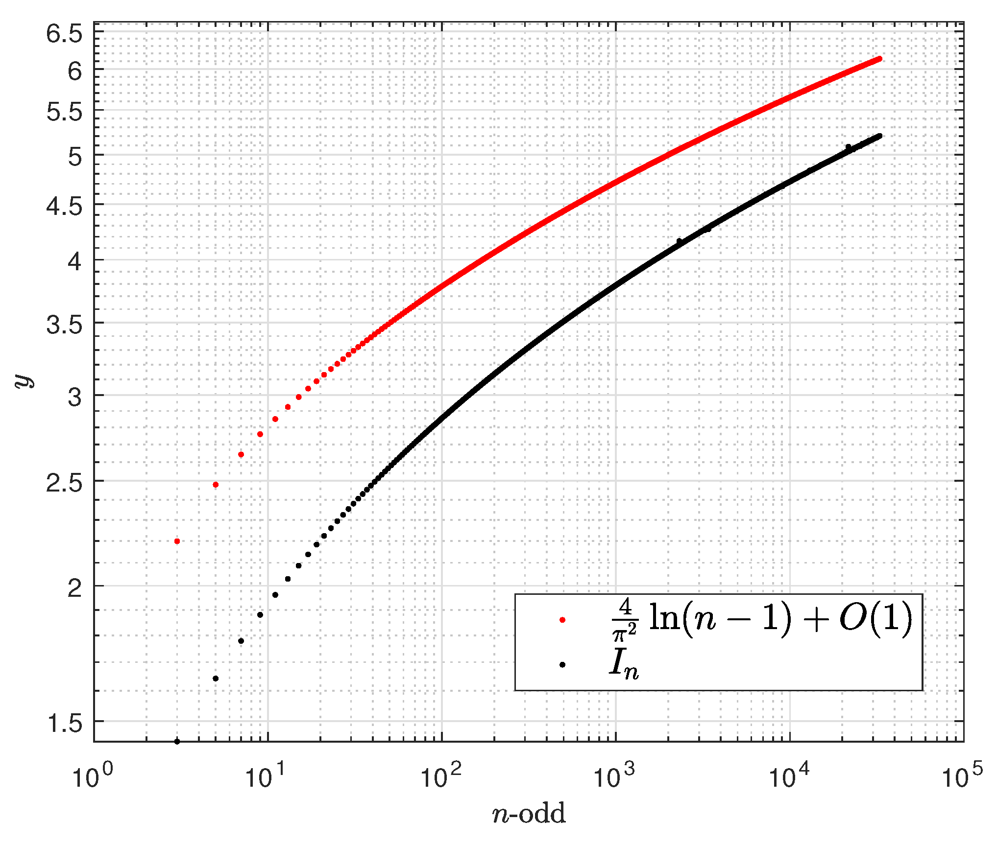
Finally, when $n\to \infty$ we obtain that [11]

$$I_n\approx {\displaystyle \frac{1}{2\pi }}{\int }_{-\pi }^{\pi }\left|D_N\left(t\right)\right|dt={\displaystyle \frac{4}{{\pi }^2}}ln(n-1)+O\left(1\right),$$

(43)

where

$$0\le O\left(1\right)\le 1+{\displaystyle \frac{2}{\pi }}+{\displaystyle \frac{4}{{\pi }^2}}ln\left(2\right).$$

(44)

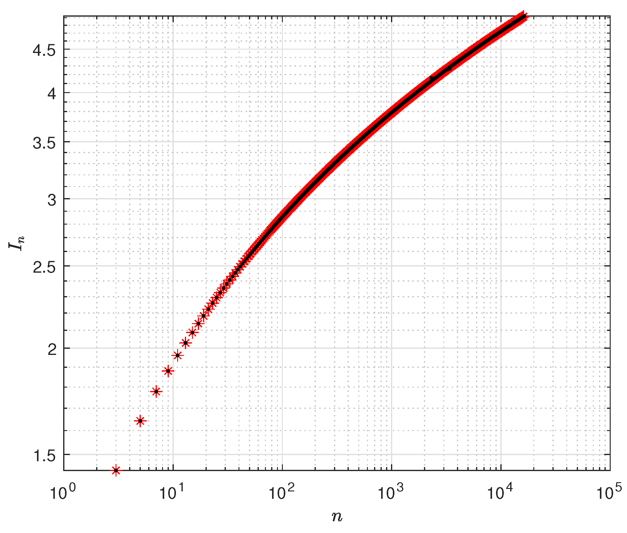
In Figure 5, we depict the extreme case when $O\left(1\right)=1+{\displaystyle \frac{2}{\pi }}+{\displaystyle \frac{4}{{\pi }^2}}ln\left(2\right)$ in (43).

Figure 5. Extreme case for odd n, when $O\left(1\right)=1+{\displaystyle \frac{2}{\pi }}+{\displaystyle \frac{4}{{\pi }^2}}ln\left(2\right)$.

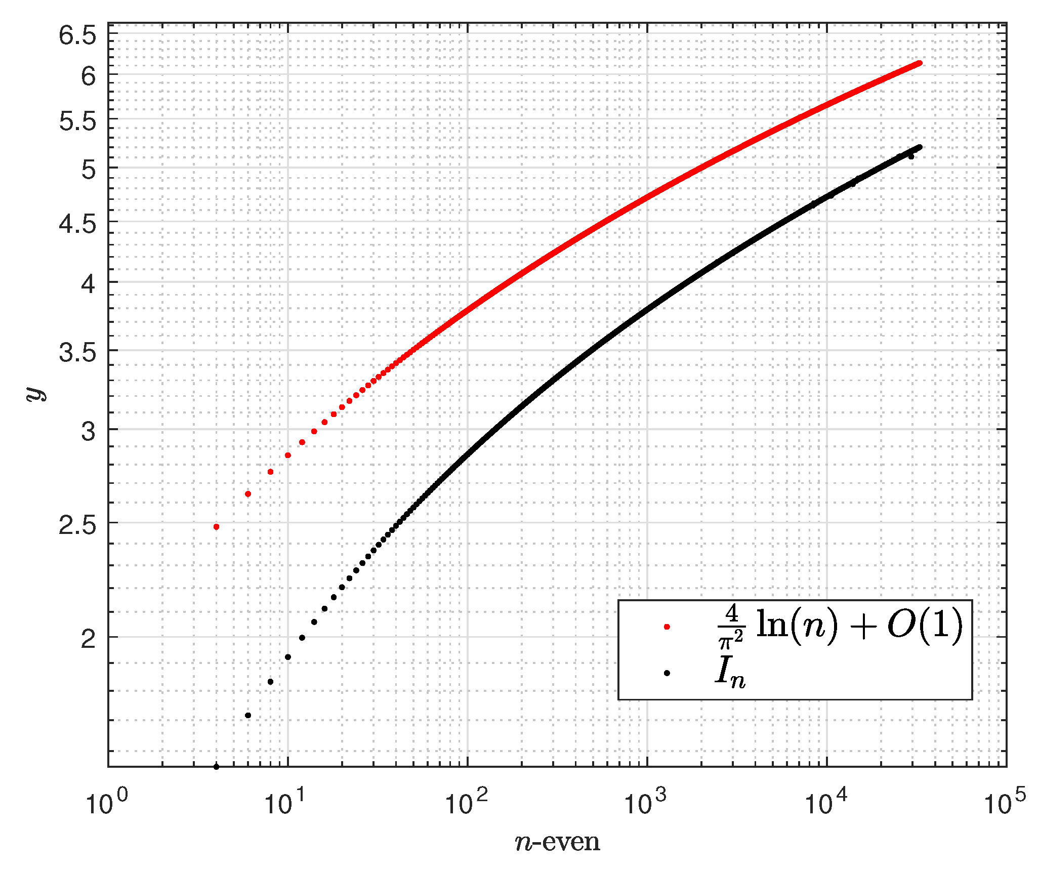
For even n cases we only need to observe that $I_n$ is a increasing function [6]; then, $I_n\le I_{n+1}$ with $n+1$ odd. From (43), we obtain that

$$I_n\approx {\displaystyle \frac{4}{{\pi }^2}}ln\left(n\right)+O\left(1\right),$$

(45)

where

$$0\le O\left(1\right)\le 1+{\displaystyle \frac{2}{\pi }}+{\displaystyle \frac{4}{{\pi }^2}}ln\left(2\right).$$

(46)

In Figure 6, we show the extreme case when $O\left(1\right)=1+{\displaystyle \frac{2}{\pi }}+{\displaystyle \frac{4}{{\pi }^2}}ln\left(2\right)$ in (45).

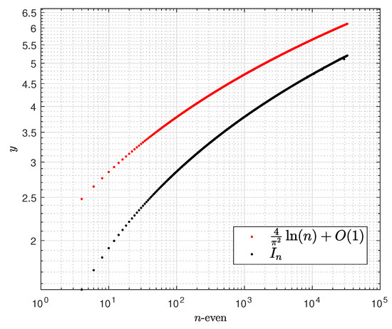
Figure 6. Extreme case for even n, when $O\left(1\right)=1+{\displaystyle \frac{2}{\pi }}+{\displaystyle \frac{4}{{\pi }^2}}ln\left(2\right)$.

References

- Finch, S. Mathematical Constants; Cambridge University Press: Cambridge, UK, 2003. [Google Scholar]
- Lebesgue, H. Sur la représentation trigonométrique approchée des fonctions satisfaisant à une condition de Lipschitz. Société Mathématique Fr. 1910, 38, 184–210. [Google Scholar] [CrossRef]
- Chen, C.; Choi, J. Inequalities and asymptotic expansions for the constants of Landau and Lebesgue. Appl. Math. Comput. 2014, 248, 610–624. [Google Scholar] [CrossRef]
- Shakirov, I.A. Approximation of the Lebesgue constant of the Fourier operator by a logarithmic-fractional-rational function. Russ. Math. 2023, 67, 64–74. [Google Scholar] [CrossRef]
- Fejér, L. Sur les singularités de la série de Fourier des fonctions continues. In Annales Scientifiques de L’École Normale Supérieure; Elsevier: Amsterdam, The Netherlands, 1911; Volume 28, pp. 63–104. [Google Scholar]
- Szego, G. Über die Lebesgueschen konstanten bei den Fourierschen reihen. Math. Z. 1921, 9, 163–166. [Google Scholar] [CrossRef]
- Watson, G. The constants of Landau and Lebesgue. Quart. J. Math. 1930, 1, 310–318. [Google Scholar] [CrossRef]
- Hardy, G. Note on Lebesgue’s constants in the theory of Fourier series. J. Lond. Math. Soc. 1942, 1, 4–13. [Google Scholar] [CrossRef]
- Zhao, D. Some sharp estimates of the constants of Landau and Lebesgue. J. Math. Anal. Appl. 2009, 349, 68–73. [Google Scholar] [CrossRef]
- Shakirov, I. Approximation of the Lebesgue constant of the Fourier operator by a logarithmic function. Russ. Math. 2022, 66, 70–76. [Google Scholar] [CrossRef]
- Alvarez, J.; Guzmán-Partida, M. Properties of the Dirichlet kernel. Electron. J. Math. Anal. Appl. 2023, 11, 96–110. [Google Scholar] [CrossRef]
- Stein, E.; Shakarchi, R. Fourier Analysis: An Introduction; Princeton University Press: Princeton, NJ, USA, 2011; Volume 1. [Google Scholar]
Disclaimer/Publisher’s Note: The statements, opinions and data contained in all publications are solely those of the individual author(s) and contributor(s) and not of MDPI and/or the editor(s). MDPI and/or the editor(s) disclaim responsibility for any injury to people or property resulting from any ideas, methods, instructions or products referred to in the content. |
© 2024 by the authors. Licensee MDPI, Basel, Switzerland. This article is an open access article distributed under the terms and conditions of the Creative Commons Attribution (CC BY) license (https://creativecommons.org/licenses/by/4.0/).