On Some Properties of the Equilateral Triangles with Vertices Located on the Support Sides of a Triangle

Abstract

The possible positions of an equilateral triangle whose vertices are located on the support sides of a generic triangle are studied. Using complex coordinates, we show that there are infinitely many such configurations, then we prove that the centroids of these equilateral triangles are collinear, defining two lines perpendicular to the Euler’s line of the original triangle. Finally, we obtain the complex coordinates of the intersection points and study some particular cases.

1. Introduction

Let $\Delta ABC$ be a triangle in the Euclidean plane, and denote the complex coordinates of the vertices A, B, and C by a, b, and c, respectively. We examine some geometric properties of the equilateral triangles $\Delta MNP$ whose vertices are located on the support sides of $\Delta ABC$, that is, $M\in BC$, $N\in AC$, and $P\in AB$.

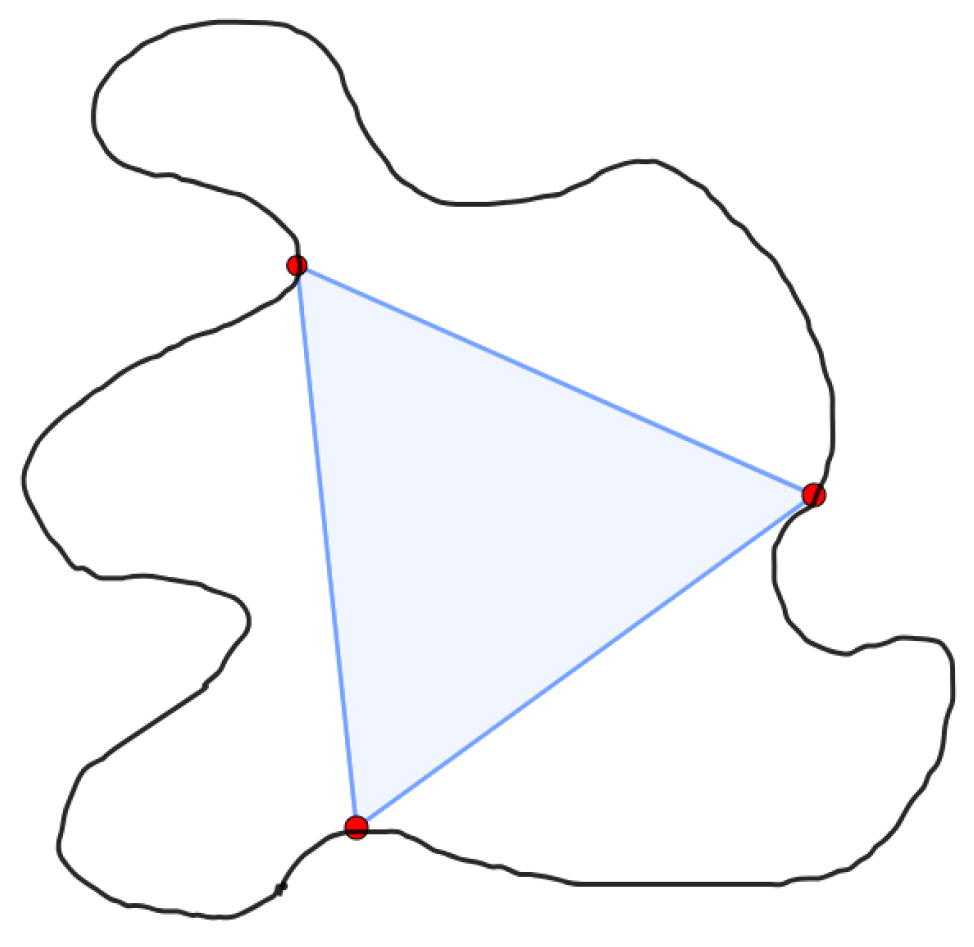
The problem studied in this paper is related to a known general topological property. The polygon $\mathcal{P}$ is said to be inscribed in the Jordan curve $\gamma$ (not necessarily contained in the interior of $\gamma$) if all the vertices of $\mathcal{P}$ are located on $\gamma$ [1]. While Jordan curves can be complicated, they satisfy certain regular properties in this respect. For example, Meyerson [2] showed that an equilateral triangle can be inscribed in every Jordan curve, as illustrated in Figure 1. Later on, Nielsen proved the following result ([3], [Theorem 1.1]): Let $J\subset {\mathbb{R}}^2$ be a Jordan curve and let Δ be any triangle. Then infinitely many triangles similar to Δ can be inscribed in γ. Similar results exist for Jordan curves in ${\mathbb{R}}^n$ [4]. Interestingly, Toeplitz’s statement from 1911 that every Jordan curve admits an inscribed square is still a conjecture in the general case. Just recently, it was proved for convex or piecewise smooth curves, while extensions exist for rectangles, curves, and Klein bottles (see, e.g., [5,6]).

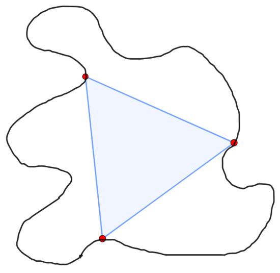
Figure 1. Inscribed equilateral triangle in a Jordan curve.

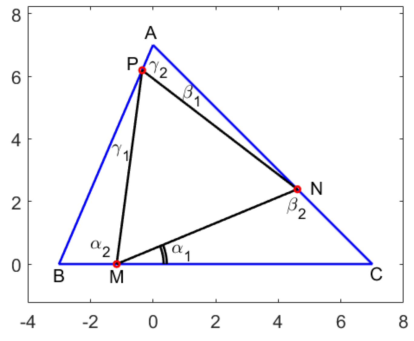
The triangle is the simplest example of a non-smooth and piecewise linear Jordan curve; while the equilateral triangle appears to be a simple configuration, it can generate very interesting properties and applications [7]. In the sense of the above definition for polygons, an equilateral triangle $MNP$ inscribed in a given triangle $ABC$ can have two vertices on the same side, a situation that does not present much interest from the geometric point of view. This is why in the present paper we consider the case $M\in BC$, $N\in CA$, and $P\in AB$, as seen in Figure 2 and Figure 3 for an acute triangle $ABC$ and in Figure 4 for an obtuse triangle, respectively. Similar to Nielsen’s result, there are infinitely many such triangles, generating interesting properties in the triangle geometry [8,9,10,11]. Recently, in [12], we studied the equilateral triangles inscribed in the interior of arbitrary triangles, describing them by a single parameter and examining some extremal properties (e.g., the angles for which the minimum inscribed equilateral triangles are obtained). A summary of the results obtained in [12] is presented in Section 2.

Figure 2. Equilateral triangle $MNP$ inscribed in the triangle $ABC$. In our example, the initial triangle has the coordinates $A(0,7)$, $B(-3,0)$, $C(7,0)$, for which the angles in degrees measure $\widehat{A}={68.1986}^{\circ }$, $\widehat{B}={66.8014}^{\circ }$, and $\widehat{C}={45}^{\circ }$, while $\widehat{M}=\widehat{N}=\widehat{P}={60}^{\circ }$.

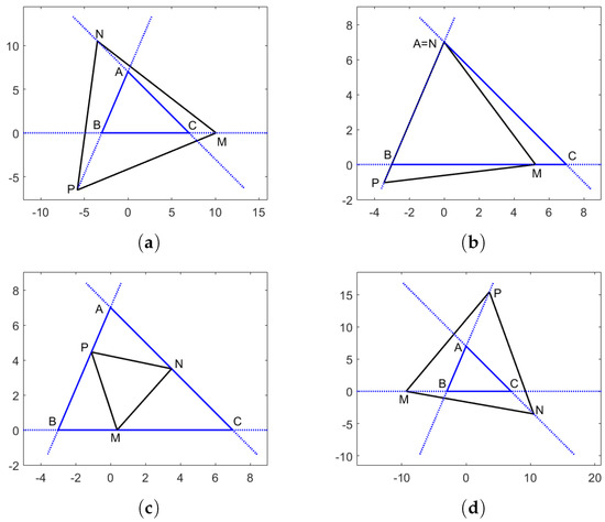
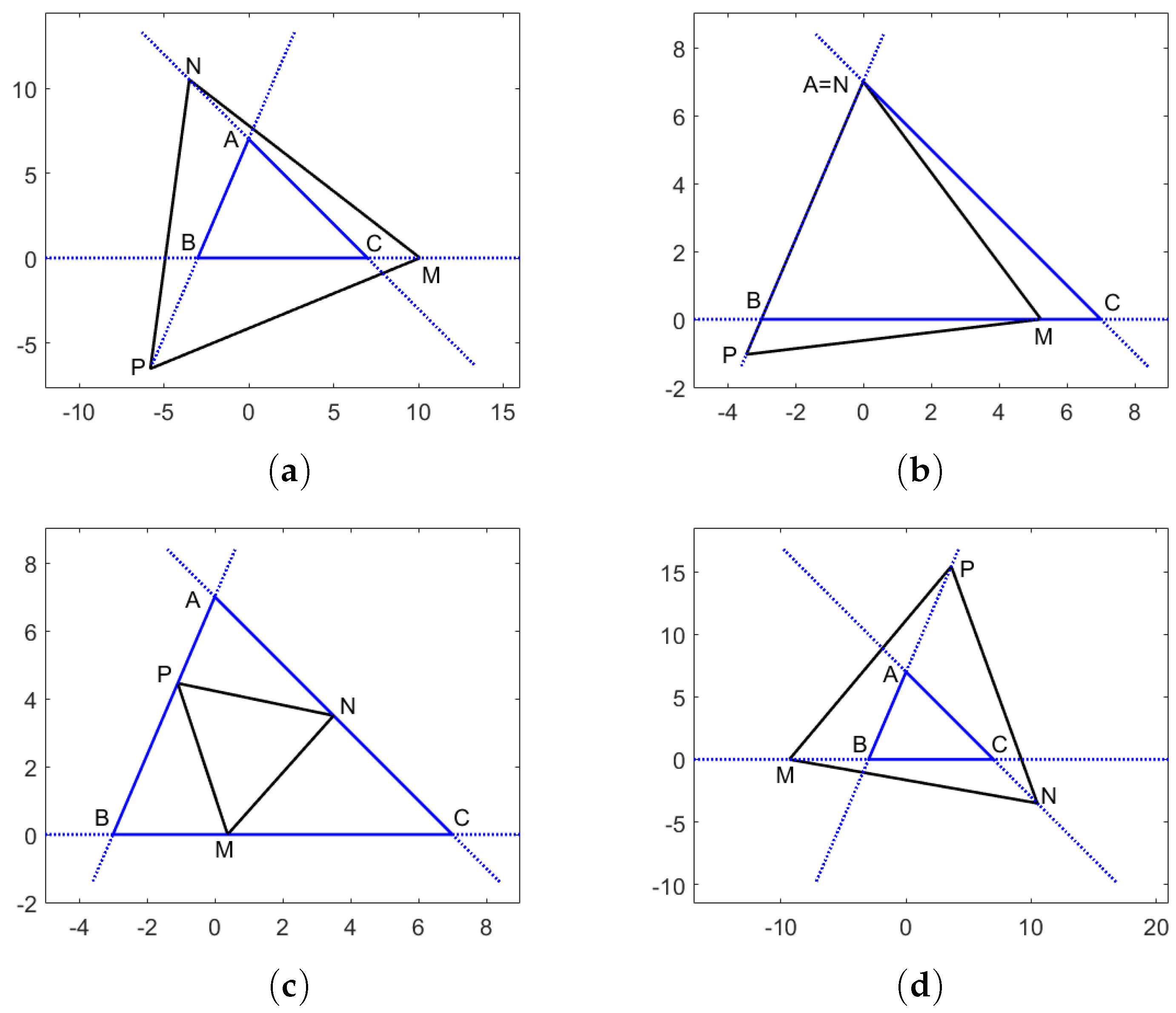
Figure 3. Figures corresponding to equilateral triangles $\Delta MNP$ with vertices on the lines $BC$, $CA$, and $AB$. (a) $\lambda =-0.5$; (b) $\lambda =0$; (c) $\lambda =0.5$; (d) $\lambda =1.5$.

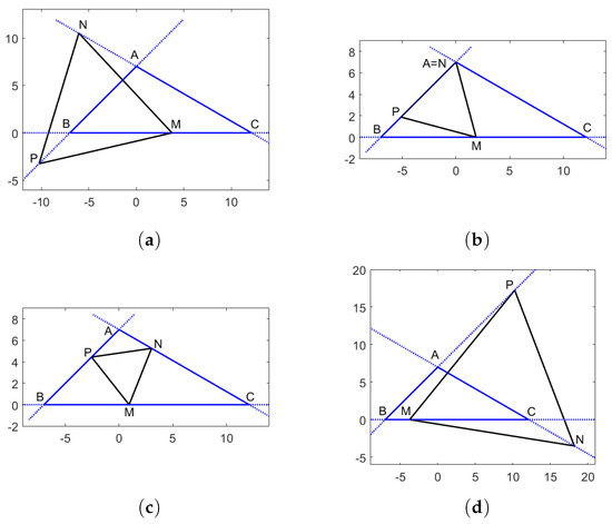
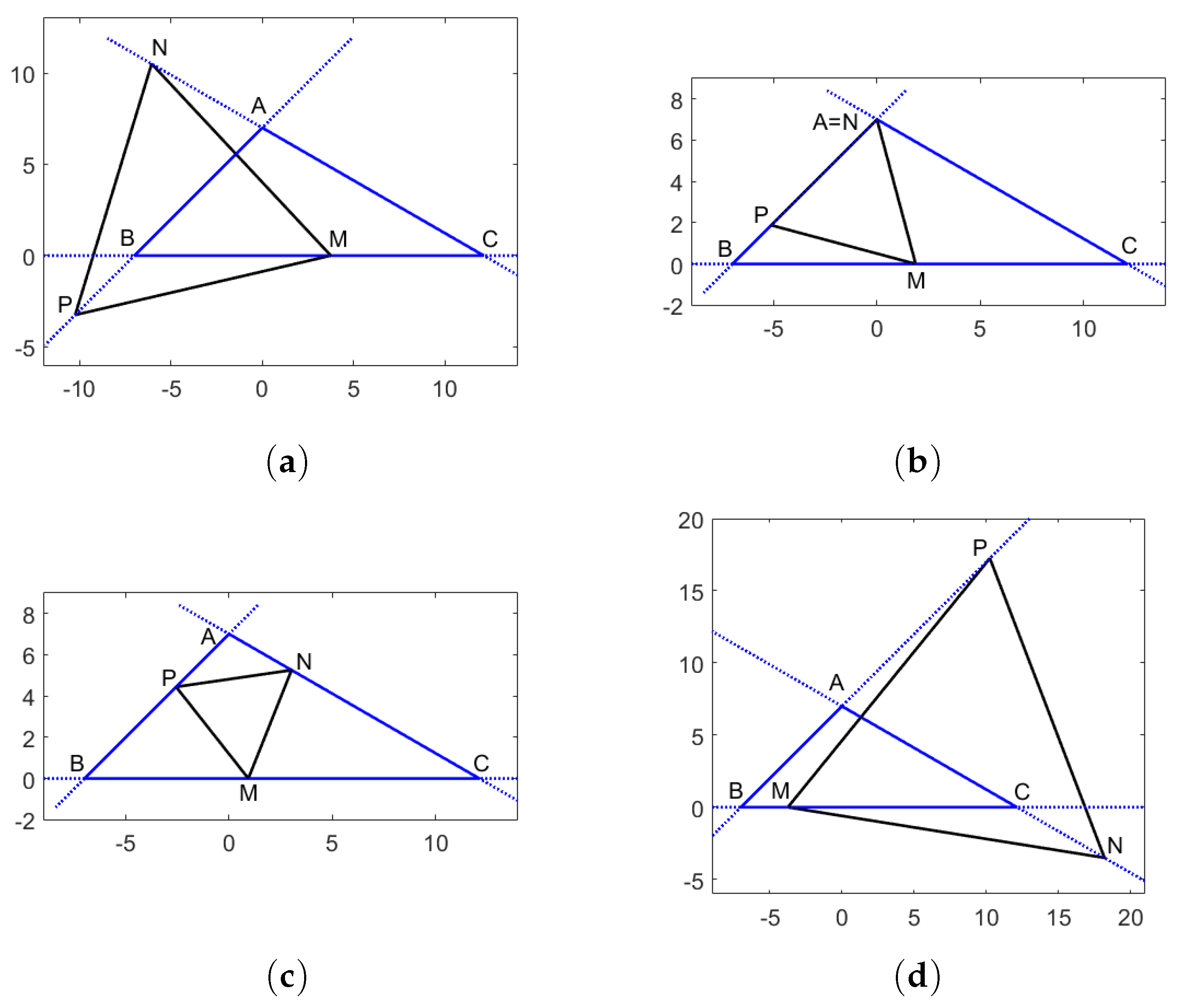
Figure 4. Figures corresponding to equilateral triangles $\Delta MNP$ with vertices on the lines $BC$, $CA$, and $AB$ of an obtuse triangle $\Delta ABC$ for (a) $\lambda =-0.5$; (b) $\lambda =0$; (c) $\lambda =0.5$; (d) $\lambda =1.5$.

In this paper, we explore the equilateral triangles whose vertices are located on the support lines of the sides of an arbitrary triangle. While this configuration does not represent a Jordan curve, this presents interesting geometric properties. We prove that the centers of these triangles are situated on two parallel lines, which are perpendicular to the Euler’s line of the original triangle.

The structure of this paper is as follows. In Section 2, we review some results obtained in [12], devoted to exact formulas for the lengths of the sides of inscribed equilateral triangles as a function of a unique parameter and to extremal properties of the side length. In Section 3, we obtain the complex coordinates of the centroids of the equilateral triangles having vertices on the support lines of a given triangle. The main result concerning the locus of these centroids is presented in Section 4. Furthermore, in Section 5 we prove that the locus of centroids consists of two parallel lines perpendicular to the Euler’s line of the original triangle. Alternative derivations and particular cases are provided in Section 6, while conclusions are formulated in Section 7.

The adoption of complex coordinates instead of Cartesian coordinates considerably simplifies the computations.

2. Inscribed Equilateral Triangles

The particular case when the inscribed equilateral triangle $MNP$ is nested, i.e., $M\in \left(BC\right)$, $N\in \left(CA\right)$, and $P\in \left(AB\right)$, was studied in [12] by a trigonometric approach. Related investigations by other means can be consulted in [8,10,11,13].

Let $\Delta ABC$ be a triangle in the Euclidean plane, and denote by A, B, and C the measures of the angles from vertices A, B, and C, respectively. Without loss of generality, one may assume that $A\ge B\ge C$; therefore, $C\le {60}^{\circ }\le A$. In the notation of Figure 2, one obtains the system

$$\begin{array}{c}\hfill \left\{\begin{array}{c}{\alpha }_1+{\alpha }_2={\displaystyle \frac{2\pi }{3}}\hfill \\ {\beta }_1+{\beta }_2={\displaystyle \frac{2\pi }{3}}\hfill \\ {\gamma }_1+{\gamma }_2={\displaystyle \frac{2\pi }{3}}\hfill \\ {\beta }_1+{\gamma }_2=\pi -A\hfill \\ {\gamma }_1+{\alpha }_2=\pi -B\hfill \\ {\alpha }_1+{\beta }_2=\pi -C.\hfill \end{array}\right.\end{array}$$

(1)

The system can be written in matrix form as

$$\begin{array}{c}\hfill \left(\begin{array}{cccccc}1& 1& 0& 0& 0& 0\\ 0& 0& 1& 1& 0& 0\\ 0& 0& 0& 0& 1& 1\\ 0& 0& 0& 1& 1& 0\\ 1& 0& 0& 0& 0& 1\\ 0& 1& 1& 0& 0& 0\end{array}\right)\left(\begin{array}{c}{\alpha }_1\\ {\alpha }_2\\ {\beta }_1\\ {\beta }_2\\ {\gamma }_1\\ {\gamma }_2\end{array}\right)=\left(\begin{array}{c}{\displaystyle \frac{2\pi }{3}}\\ {\displaystyle \frac{2\pi }{3}}\\ {\displaystyle \frac{2\pi }{3}}\\ \pi -A\\ \pi -B\\ \pi -C\end{array}\right).\end{array}$$

(2)

By simple calculation, one can show that the system (2) is compatible and it has infinitely many solutions. Moreover, since the rank of the matrix is 5, the solutions are fully determined by a single variable chosen as the parameter. From the first three equations, one can substitute ${\alpha }_2$, ${\beta }_2$, and ${\gamma }_2$ into the last three and obtain the reduced system

$$\left\{\begin{array}{c}{\gamma }_1-{\beta }_1={\displaystyle \frac{\pi }{3}}-A\hfill \\ {\alpha }_1-{\gamma }_1={\displaystyle \frac{\pi }{3}}-B\hfill \\ {\beta }_1-{\alpha }_1={\displaystyle \frac{\pi }{3}}-C,\hfill \end{array}\right.$$

(3)

which can be written in matrix form as

$$\begin{array}{c}\hfill \left(\begin{array}{ccc}0& -1& 1\\ 1& 0& -1\\ -1& 1& 0\end{array}\right)\left(\begin{array}{c}{\alpha }_1\\ {\beta }_1\\ {\gamma }_1\end{array}\right)=\left(\begin{array}{c}{\displaystyle \frac{\pi }{3}}-A\\ {\displaystyle \frac{\pi }{3}}-B\\ {\displaystyle \frac{\pi }{3}}-C\end{array}\right).\end{array}$$

(4)

Fixing the parameter ${\alpha }_1=\alpha \in [0,{120}^{\circ }]=m(\angle NMC)$, the system (3) has the solution

$${\beta }_1=\alpha +C-{60}^{\circ },{\gamma }_1=\alpha +{60}^{\circ }-B.$$

From the conditions $0\le {\beta }_1,{\gamma }_1\le {120}^{\circ }$ one obtains $\alpha +{60}^{\circ }-B\le {120}^{\circ }$. The geometric constraints illustrated in Figure 2

$$\begin{array}{c}\hfill {60}^{\circ }-C\le \alpha \le min\{{60}^{\circ }+B,{120}^{\circ }\},\end{array}$$

(5)

show that there are infinitely many possible configurations.

In our recent paper [12], we obtained the following explicit formula for the side length of the inscribed equilateral triangle as a function of the parameter $\alpha$:

$$\begin{array}{cc}\hfill l\left(\alpha \right)& ={\displaystyle \frac{2R·sinA·sinB·sinC}{sinC·sin\left(\alpha +{60}^{\circ }-B\right)+sinB·sin\left(\alpha +C\right)}}\hfill \\ \hfill & ={\displaystyle \frac{2R·sinA·sinB·sinC}{sinA·sin\alpha +sinC·sin\left({60}^{\circ }+B-\alpha \right)}}\hfill \\ \hfill & ={\displaystyle \frac{2R·sinA·sinB·sinC}{sinB·sin\left(\alpha +C-{60}^{\circ }\right)+sinA·sin\left(\alpha +{60}^{\circ }\right)}},\hfill \end{array}$$

where R is the circumradius of triangle $ABC$. Denote $K\left[ABC\right]$ as the area of triangle $ABC$, and from the relation $K\left[ABC\right]={\displaystyle \frac{AB·BC·CA}{4R^2}}$ and the Law of Sines, one obtains

$$\begin{array}{cc}\hfill l\left(\alpha \right)& ={\displaystyle \frac{2K\left[ABC\right]}{AB·sin\left(\alpha +{60}^{\circ }-B\right)+AC·sin\left(\alpha +C\right)}}\hfill \\ \hfill & ={\displaystyle \frac{2K\left[ABC\right]}{BC·sin\alpha +AB·sin\left({60}^{\circ }+B-\alpha \right)}}\hfill \\ \hfill & ={\displaystyle \frac{2K\left[ABC\right]}{AC·sin\left(\alpha +C-{60}^{\circ }\right)+BC·sin\left(\alpha +{60}^{\circ }\right)}}.\hfill \end{array}$$

(6)

Furthermore, we showed in [12] that the minimal triangle $MNP$ is obtained for

$$\begin{array}{c}\hfill {\alpha }^{*}=arctan{\displaystyle \frac{\frac{\sqrt{3}}{2}sinB·sinC+\frac{1}{2}cosBsinC+sinBcosC}{\frac{\sqrt{3}}{2}cosBsinC+\frac{1}{2}sinBsinC}}.\end{array}$$

Numerous illustrative examples are also provided in [12].

3. Coordinates of the Centroids of the Triangle MNP

The complex coordinates of the vertices of $\Delta MNP$ are denoted by m, n, and p. As seen in Figure 3 for an acute triangle and in Figure 4 for an obtuse triangle, such triangles can be constructed starting from the points N on $AC$ and P on the side $AB$, with the condition that the third point M on $BC$ is obtained by a rotation of angle $\pi /3$, which in complex numbers can be performed by multiplying with (see, for example, [14]):

$$\omega =cos{\displaystyle \frac{\pi }{3}}+isin{\displaystyle \frac{\pi }{3}}={\displaystyle \frac{1}{2}}+{\displaystyle \frac{\sqrt{3}}{2}}i.$$

Clearly, if $N\in AC$ and $P\in AB$, there exist the scalars $\lambda$ and $\mu$ such that

$$n=a+\lambda (c-a),p=a+\mu (b-a),\lambda ,\mu \in \mathbb{R}.$$

In this notation, note that, as seen in Figure 3, we have

• If $\lambda <0$, then $A\in \left(NC\right)$;
• If $\lambda =0$, then $A=N$;
• If $0<\lambda <1$, then $N\in \left(AC\right)$ (the case presented in Section 2);
• If $\lambda =1$, then $N=C$;
• If $\lambda >1$, then $C\in \left(AN\right)$.

Then, the point M of the equilateral triangle $MNP$ is obtained by rotating segment $\left(PN\right)$ around point N through an angle of $\pi /3$, clockwise or anticlockwise.

3.1. First Orientation of Triangle MNP: Anticlockwise Rotation

For anticlockwise rotation, we obtain the complex coordinate

$$\begin{array}{cc}\hfill m& =n+\left(p-n\right)\omega \hfill \\ \hfill & =\left[\left(1-\mu \right)a+\mu b\right]\omega +\left[\left(1-\lambda \right)a+\lambda c\right]\overline{\omega }\hfill \\ \hfill & =a+\mu \omega \left(b-a\right)+\lambda \overline{\omega }\left(c-a\right)=c+s\left(b-c\right),\hfill \end{array}$$

where we use the relation $\omega +\overline{\omega }=1$. Since $M\in \left(BC\right)$, one must have $s\in \mathbb{R}$, hence $s=\overline{s}$. From here it follows that

$$\begin{array}{cc}\hfill s& ={\displaystyle \frac{a-c+\mu \omega \left(b-a\right)+\lambda \overline{\omega }\left(c-a\right)}{b-c}}\hfill \\ \hfill & ={\displaystyle \frac{\overline{a}-\overline{c}+\mu \overline{\omega }\left(\overline{b}-\overline{a}\right)+\lambda \omega \left(\overline{c}-\overline{a}\right)}{\overline{b}-\overline{c}}}=\overline{s}.\hfill \end{array}$$

This condition can be written as

$$\begin{array}{c}\hfill \left[\left(a-c\right)+\mu \omega \left(b-a\right)+\lambda \overline{\omega }\left(c-a\right)\right]\left(\overline{b}-\overline{c}\right)=\left[\left(\overline{a}-\overline{c}\right)+\mu \overline{\omega }\left(\overline{b}-\overline{a}\right)+\lambda \omega \left(\overline{c}-\overline{a}\right)\right]\left(b-c\right),\end{array}$$

which reduces to

$$\begin{array}{c}\hfill \mu ={\displaystyle \frac{y}{x}}\lambda +{\displaystyle \frac{z}{x}}=k\lambda +l,\end{array}$$

(7)

where x, y, and z are given by

$$\begin{array}{cc}\hfill x& =\omega \left(b-a\right)\left(\overline{b}-\overline{c}\right)-\overline{\omega }\left(\overline{b}-\overline{a}\right)\left(b-c\right)\in i·\mathbb{R},\hfill \\ \hfill y& =\omega \left(b-c\right)\left(\overline{c}-\overline{a}\right)-\overline{\omega }\left(\overline{b}-\overline{c}\right)\left(c-a\right)\in i·\mathbb{R},\hfill \\ \hfill z& =\left(b-c\right)\left(\overline{a}-\overline{c}\right)-\left(\overline{b}-\overline{c}\right)\left(a-c\right)\in i·\mathbb{R}.\hfill \end{array}$$

(8)

Clearly, this shows that the coordinates m, n, p depend linearly on $\lambda \in \mathbb{R}$, as

$$\begin{array}{cc}\hfill n\left(\lambda \right)& =a+\lambda \left(c-a\right),\hfill \\ \hfill p\left(\lambda \right)& =a+\left(k\lambda +l\right)\left(b-a\right),\hfill \\ \hfill m\left(\lambda \right)& =a+\left(k\lambda +l\right)\omega \left(b-a\right)+\lambda \overline{\omega }\left(c-a\right),\lambda \in \mathbb{R},\hfill \end{array}$$

where the values k and l are real numbers obtained from (7) and (8), as

$$\begin{array}{cc}\hfill k& ={\displaystyle \frac{\omega \left(b-c\right)\left(\overline{c}-\overline{a}\right)-\overline{\omega }\left(\overline{b}-\overline{c}\right)\left(c-a\right)}{\omega \left(b-a\right)\left(\overline{b}-\overline{c}\right)-\overline{\omega }\left(\overline{b}-\overline{a}\right)\left(b-c\right)}},\hfill \\ \hfill l& ={\displaystyle \frac{\left(b-c\right)\left(\overline{a}-\overline{c}\right)-\left(\overline{b}-\overline{c}\right)\left(a-c\right)}{\omega \left(b-a\right)\left(\overline{b}-\overline{c}\right)-\overline{\omega }\left(\overline{b}-\overline{a}\right)\left(b-c\right)}},\hfill \end{array}$$

(9)

which are ratios of purely imaginary numbers.

3.2. Second Orientation of Triangle MNP: Clockwise Rotation

An alternative configuration is obtained when the rotation of P around N is taken with an angle of ${60}^{\circ }$ clockwise. Similar to Section 3.1, we obtain

$$\begin{array}{cc}\hfill m_2& =n+\left(p_2-n\right)\overline{\omega }\hfill \\ \hfill & =\left[\left(1-\mu \right)a+\mu b\right]\overline{\omega }+\left[\left(1-\lambda \right)a+\lambda c\right]\omega \hfill \\ \hfill & =a+\mu \overline{\omega }\left(b-a\right)+\lambda \omega \left(c-a\right)=c+s\left(b-c\right),\hfill \end{array}$$

where we use the fact that $\omega +\overline{\omega }=1$. Imposing the condition $s=\overline{s}$, for $\lambda \in \mathbb{R}$, the coordinates of the vertices of $\Delta MNP$ can be written explicitly

$$\begin{array}{cc}\hfill n\left(\lambda \right)& =a+\lambda \left(c-a\right),\hfill \\ \hfill p_2\left(\lambda \right)& =a+\left(k_2\lambda +l_2\right)\left(b-a\right),\hfill \\ \hfill m_2\left(\lambda \right)& =a+\left(k_2\lambda +l_2\right)\overline{\omega }\left(b-a\right)+\lambda \omega \left(c-a\right).\hfill \end{array}$$

(10)

The coefficients are related through the formula

$$\begin{array}{c}\hfill {\mu }_2={\displaystyle \frac{y_2}{x_2}}\lambda +{\displaystyle \frac{z_2}{x_2}}=k_2\lambda +l_2,\end{array}$$

(11)

where $x_2$, $y_2$, and $z_2$ are obtained from

$$\begin{array}{cc}\hfill x_2& =\overline{\omega }\left(b-a\right)\left(\overline{b}-\overline{c}\right)-\omega \left(\overline{b}-\overline{a}\right)\left(b-c\right)\in i·\mathbb{R},\hfill \\ \hfill y_2& =\overline{\omega }\left(b-c\right)\left(\overline{c}-\overline{a}\right)-\omega \left(\overline{b}-\overline{c}\right)\left(c-a\right)\in i·\mathbb{R},\hfill \\ \hfill z_2& =\left(b-c\right)\left(\overline{a}-\overline{c}\right)-\left(\overline{b}-\overline{c}\right)\left(a-c\right)=z.\hfill \end{array}$$

(12)

Using (11) and (12), the values $k_2$ and $l_2$ are the real numbers given by

$$\begin{array}{cc}\hfill k_2& ={\displaystyle \frac{\overline{\omega }\left(b-c\right)\left(\overline{c}-\overline{a}\right)-\omega \left(\overline{b}-\overline{c}\right)\left(c-a\right)}{\overline{\omega }\left(b-a\right)\left(\overline{b}-\overline{c}\right)-\omega \left(\overline{b}-\overline{a}\right)\left(b-c\right)}},\hfill \\ \hfill l_2& ={\displaystyle \frac{\left(b-c\right)\left(\overline{a}-\overline{c}\right)-\left(\overline{b}-\overline{c}\right)\left(a-c\right)}{\overline{\omega }\left(b-a\right)\left(\overline{b}-\overline{c}\right)-\omega \left(\overline{b}-\overline{a}\right)\left(b-c\right)}}.\hfill \end{array}$$

(13)

These formulas allow a convenient calculation for the coordinates of the centroids.

For a given point $N\in AC$, the possible equilateral triangles are shown in Figure 5.

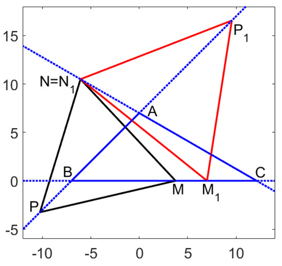
Figure 5. Inscribed equilateral triangles with distinct orientations.

4. The Collinearity of the Centroids of Triangle MNP

In this section, we show that for each orientation of the triangles $MNP$ (clockwise and anticlockwise), the corresponding centroids are collinear.

4.1. The First Line of Centroids

As a function of $\lambda$, the coordinate of the centroid of triangle $\Delta MNP$ is given by

$$\begin{array}{cc}\hfill g_1\left(\lambda \right)& ={\displaystyle \frac{m+n+p}{3}}\hfill \\ \hfill & ={\displaystyle \frac{\left[a+\mu \omega \left(b-a\right)+\lambda \overline{\omega }\left(c-a\right)\right]+\left[a+\lambda (c-a)\right]+\left[a+\mu (b-a)\right]}{3}}\hfill \\ \hfill & =a+{\displaystyle \frac{\mu \left(1+\omega \right)\left(b-a\right)+\lambda \left(1+\overline{\omega }\right)\left(c-a\right)}{3}}\hfill \\ \hfill & =\left[k\left(1+\omega \right)\left(b-a\right)+\left(1+\overline{\omega }\right)\left(c-a\right)\right]·{\displaystyle \frac{\lambda }{3}}+{\displaystyle \frac{l\left(1+\omega \right)\left(b-a\right)}{3}}+a,\hfill \end{array}$$

(14)

where we use (7) for k and l. By this formula, it follows that the centroids of the equilateral triangles $\Delta MNP$ situated on the support lines $BC$, $CA$, and $AB$, are collinear, as depicted in Figure 6 and Figure 7, for a specified range of values $\lambda$.

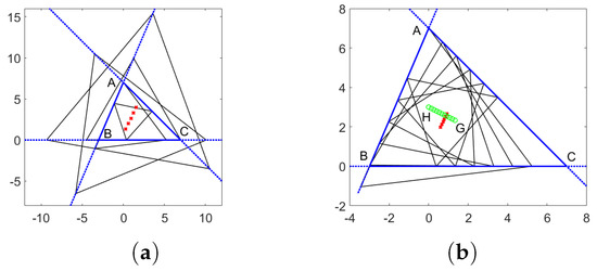
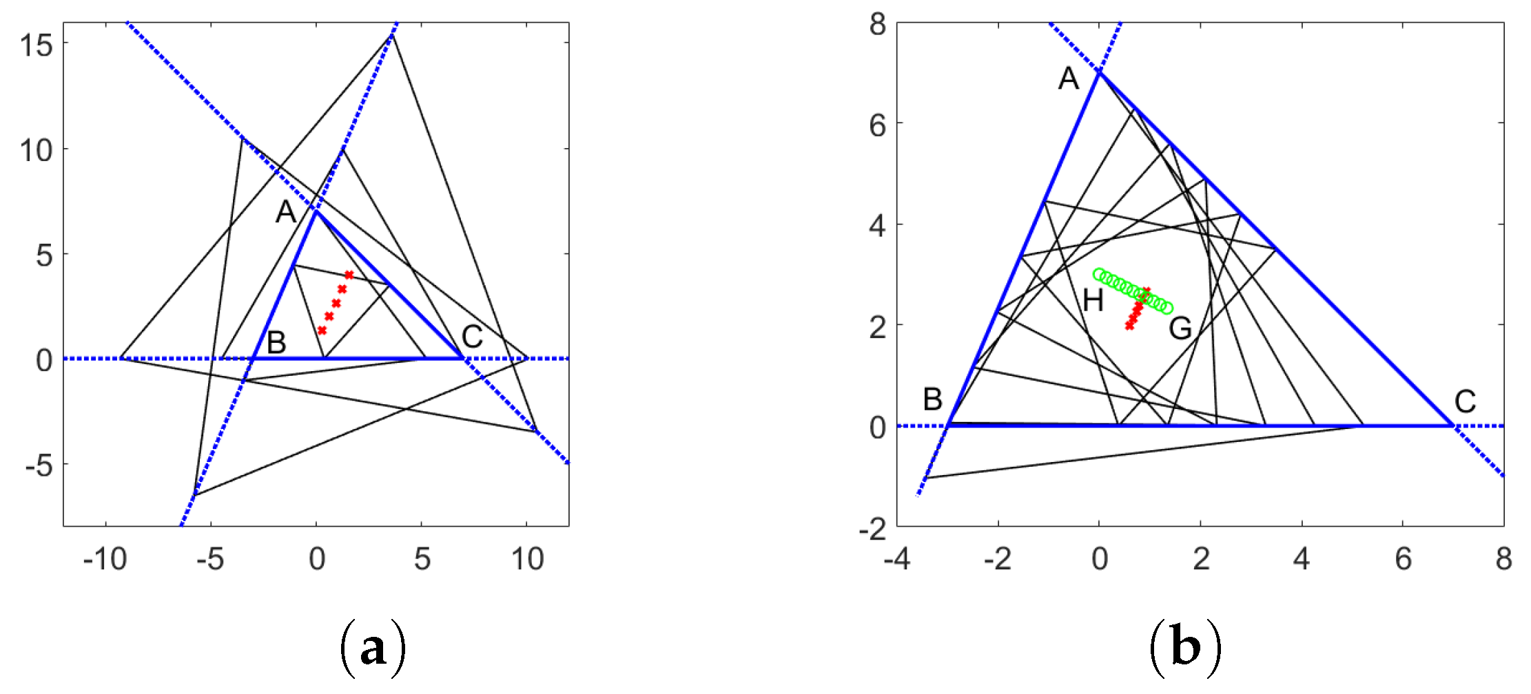
Figure 6. Equilateral triangles $\Delta MNP$ with the vertices on the lines $BC$, $CA$, and $AB$, with centroids represented by red “x” symbols. (a) $\lambda$ = −0.5, 0, 0.5, 1, 1.5; (b) $\lambda$ = 0, 0.1, 0.2, 0.3, 0.4, 0.5. Also plotted are the centroid G and orthocenter H of $\Delta ABC$.

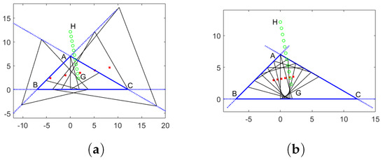
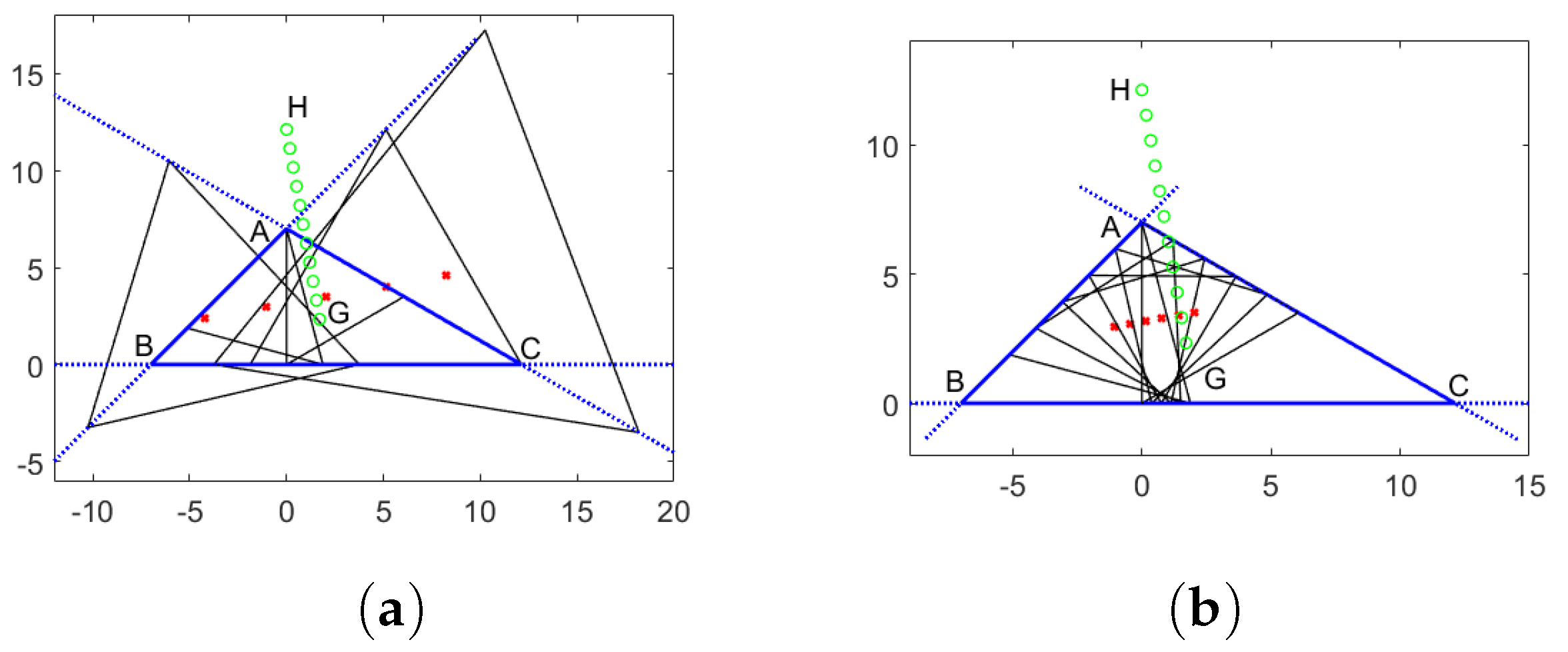
Figure 7. Equilateral triangles $\Delta MNP$ with the vertices on the lines $BC$, $CA$, and $AB$, with centroids represented by red “x” symbols. (a) $\lambda =-$0.5, 0, 0.5, 1, 1.5; (b) $\lambda =$ 0, 0.1, 0.2, 0.3, 0.4, 0.5. Also plotted are the centroid G and orthocenter H of $\Delta ABC$.

4.2. The Second Line of Centroids

For the second line, using (10), we have the formula

$$\begin{array}{cc}\hfill g_2\left(\lambda \right)& ={\displaystyle \frac{m_2+n+p_2}{3}}\hfill \\ \hfill & ={\displaystyle \frac{\left[a+{\mu }_2\overline{\omega }\left(b-a\right)+\lambda \omega \left(c-a\right)\right]+\left[a+\lambda (c-a)\right]+\left[a+{\mu }_2(b-a)\right]}{3}}\hfill \\ \hfill & =a+{\displaystyle \frac{{\mu }_2\left(1+\overline{\omega }\right)\left(b-a\right)+\lambda \left(1+\omega \right)\left(c-a\right)}{3}}\hfill \\ \hfill & =\left[k_2\left(1+\overline{\omega }\right)\left(b-a\right)+\left(1+\omega \right)\left(c-a\right)\right]·{\displaystyle \frac{\lambda }{3}}+{\displaystyle \frac{l_2\left(1+\overline{\omega }\right)\left(b-a\right)}{3}}+a,\hfill \end{array}$$

(15)

where we use (11) and the coefficients $k_2$ and $l_2$ given by (13).

5. Perpendicularity and Intersection with Euler’s Line

The following auxiliary result is useful in proving the main results of this section.

Lemma 1. 

Let $u_1$, $u_2$, $v_1$, and $v_2$ be complex numbers and consider the lines $\left({\alpha }_1\right)$ and $\left({\alpha }_2\right)$ given in parametric form by $z=u_{1}t+v_1$, $t\in \mathbb{R}$ and $\zeta =u_{2}s+v_2$, $s\in \mathbb{R}$, respectively. The following properties hold:

(1) 

If $\overline{u_1}{u}_2+u_1\overline{u_2}=0$, then $\left({\alpha }_1\right)$ and $\left({\alpha }_2\right)$ are perpendicular.

(2) 

If $\overline{u_1}{u}_2-u_1\overline{u_2}\ne 0$, then $\left({\alpha }_1\right)$ and $\left({\alpha }_2\right)$ intersect at the point

$$\begin{array}{c}\hfill Z={\displaystyle \frac{u_1\left(u_2\overline{v_2}-\overline{u_2}{v}_2\right)-u_2\left(u_1\overline{v_1}-\overline{u_1}{v}_1\right)}{\overline{u_1}{u}_2-u_1\overline{u_2}}}.\end{array}$$

(16)

Proof. 

$\left(1\right)$ Let us consider the points $z^{\prime }=u_1{t}_1+v_1$ and $z^{″}=u_1{t}_2+v_1$ on $\left({\alpha }_1\right)$ and the points ${\zeta }^{\prime }=u_2{s}_1+v_2$ and ${\zeta }^{″}=u_2{s}_2+v_2$ on $\left({\alpha }_2\right)$. The lines are perpendicular if and only if

$$\begin{array}{c}\hfill {\displaystyle \frac{{\zeta }^{″}-{\zeta }^{\prime }}{z^{″}-z^{\prime }}}={\displaystyle \frac{\left(u_2{s}_2+v_2\right)-\left(u_2{s}_1+v_2\right)}{\left(u_1{t}_2+v_1\right)-\left(u_1{t}_1+v_1\right)}}={\displaystyle \frac{u_2\left(s_2-s_1\right)}{u_1\left(t_2-t_1\right)}}\in i·\mathbb{R},\end{array}$$

which reduces to ${\displaystyle \frac{u_2}{u_1}}\in i·\mathbb{R}$. Therefore,

$$\begin{array}{c}\hfill 0={\displaystyle \frac{u_2}{u_1}}+\overline{\left({\displaystyle \frac{u_2}{u_1}}\right)}={\displaystyle \frac{u_2}{u_1}}+{\displaystyle \frac{\overline{u_2}}{\overline{u_1}}}={\displaystyle \frac{\overline{u_1}{u}_2+u_1\overline{u_2}}{|u_1{|}^2}}=0,\end{array}$$

from where the conclusion follows.

$\left(2\right)$ If the point of coordinate Z is located on both lines, it means that there exist real numbers t and s such that $Z=u_{1}t+v_1=u_{2}s+v_2$. By conjugation, one obtains $\overline{u_1}t+\overline{v_1}=\overline{u_2}s+\overline{v_2}$, from where we can solve for t and s the system

$$\left\{\begin{array}{c}{u}_{2}s-u_{1}t=v_1-v_2\hfill \\ \overline{u_2}s-\overline{u_1}t=\overline{v_1}-\overline{v_2}.\hfill \end{array}\right.$$

(17)

The system (17) has the solution

$$\begin{array}{c}\hfill s={\displaystyle \frac{\overline{u_1}\left(v_1-v_2\right)-u_1\left(\overline{v_1}-\overline{v_2}\right)}{\left(\overline{u_1}{u}_2-u_1\overline{u_2}\right)}},t={\displaystyle \frac{\overline{u_2}\left(v_1-v_2\right)-u_2\left(\overline{v_1}-\overline{v_2}\right)}{\left(\overline{u_1}{u}_2-u_1\overline{u_2}\right)}},\end{array}$$

and by substitution, one obtains

$$\begin{array}{c}\hfill Z=u_{1}t+v_1=u_1·{\displaystyle \frac{\overline{u_2}\left(v_1-v_2\right)-u_2\left(\overline{v_1}-\overline{v_2}\right)}{\left(\overline{u_1}{u}_2-u_1\overline{u_2}\right)}}+v_1,\end{array}$$

which after simplifications recovers formula (16). □

A special case is when $\left({\alpha }_2\right)$ passes through the origin.

Recall that in every triangle $ABC$, the circumcenter O, the centroid G, and the orthocenter H are collinear on the Euler line of the triangle. Without loss of generality, we can choose the circumcenter O of $\Delta ABC$ as the origin of the complex plane. Under this assumption, we obtain the coordinates $o=0$, $g={\displaystyle \frac{a+b+c}{3}}$, and $h=a+b+c$; hence, Euler’s line is defined by the formula $u\left(a+b+c\right)$, $u\in \mathbb{R}$. Furthermore, the circumradius of the triangle $ABC$ can be set to 1, in which case we have $\left|a\right|=\left|b\right|=\left|c\right|=1$, or

$$\overline{a}={\displaystyle \frac{1}{a}},\overline{b}={\displaystyle \frac{1}{b}},\overline{c}={\displaystyle \frac{1}{c}}.$$

5.1. The First Line of Centroids

For the first centroid line, by substituting, we obtain

$$\begin{array}{cc}\hfill x& =\omega \left(b-a\right)\left({\displaystyle \frac{1}{b}}-{\displaystyle \frac{1}{c}}\right)-\overline{\omega }\left({\displaystyle \frac{1}{b}}-{\displaystyle \frac{1}{a}}\right)\left(b-c\right)\hfill \\ \hfill & ={\displaystyle \frac{1}{abc}}\left(b-a\right)\left(c-b\right)\left(\omega a-\overline{\omega }c\right)\hfill \\ \hfill y& =\omega \left(b-c\right)\left({\displaystyle \frac{1}{c}}-{\displaystyle \frac{1}{a}}\right)-\overline{\omega }\left({\displaystyle \frac{1}{b}}-{\displaystyle \frac{1}{c}}\right)\left(c-a\right)\hfill \\ \hfill & ={\displaystyle \frac{1}{abc}}\left(b-c\right)\left(a-c\right)\left(\omega b-\overline{\omega }a\right)={\displaystyle \frac{1}{abc}}\left(c-b\right)\left(c-a\right)\left(\omega b-\overline{\omega }a\right)\hfill \\ \hfill z& =\left(b-c\right)\left({\displaystyle \frac{1}{a}}-{\displaystyle \frac{1}{c}}\right)-\left({\displaystyle \frac{1}{b}}-{\displaystyle \frac{1}{c}}\right)\left(a-c\right)\hfill \\ \hfill & ={\displaystyle \frac{1}{abc}}\left(b-a\right)\left(b-c\right)\left(c-a\right)={\displaystyle \frac{1}{abc}}\left(b-a\right)\left(c-b\right)\left(a-c\right).\hfill \end{array}$$

Substituting in (7), we obtain

$$\begin{array}{cc}\hfill k& ={\displaystyle \frac{y}{x}}={\displaystyle \frac{c-a}{b-a}}·{\displaystyle \frac{\omega b-\overline{\omega }a}{\omega a-\overline{\omega }c}},\hfill \end{array}$$

(18)

$$\begin{array}{cc}\hfill l& ={\displaystyle \frac{z}{x}}={\displaystyle \frac{a-c}{\omega a-\overline{\omega }c}}.\hfill \end{array}$$

(19)

Therefore, the first line of centroids depicted in Figure 8 has the equation

$$\begin{array}{cc}\hfill g_1\left(\lambda \right)& ={\displaystyle \frac{c-a}{\omega a-\overline{\omega }c}}·\left(a+b+c\right)·\sqrt{3}i·{\displaystyle \frac{\lambda }{3}}+{\displaystyle \frac{a-c}{\omega a-\overline{\omega }c}}·{\displaystyle \frac{\left(1+\omega \right)\left(b-a\right)}{3}}+a\hfill \\ \hfill & =-\left(a+b+c\right)·\lambda \sqrt{3}i·{\displaystyle \frac{l}{3}}+{\displaystyle \frac{l\left(1+\omega \right)\left(b-a\right)}{3}}+a=u_1\lambda +v_1,\hfill \end{array}$$

(20)

while Euler’s line is given by

$$\begin{array}{c}\hfill E\left(s\right)=(a+b+c)s=u_{2}s+v_2.\end{array}$$

(21)

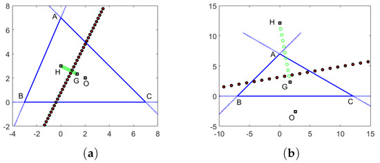
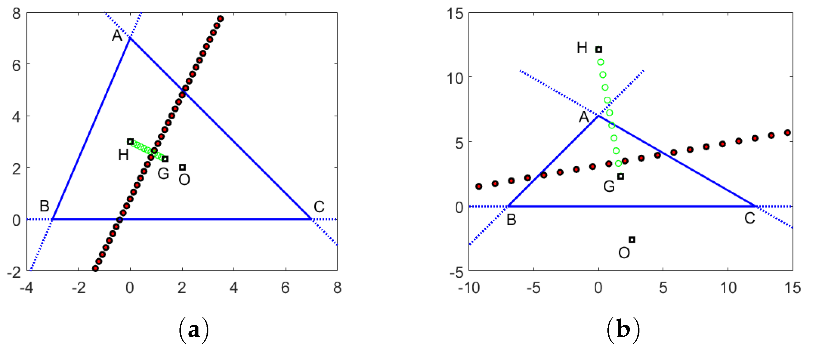
Figure 8. First line of centroids $g_1\left(\lambda \right)$ given by (14), represented by red “x” symbols. (a) Acute triangle; (b) obtuse triangle. Also plotted are the centroid G, orthocenter H, and centre O of $\Delta ABC$.

By Formulas (20) and (21) for the line of centroids and Euler’s line, we obtain

$$\begin{array}{cc}\hfill u_1& =-\left(a+b+c\right)·\sqrt{3}i·{\displaystyle \frac{l}{3}},\hfill \\ \hfill v_1& ={\displaystyle \frac{l\left(1+\omega \right)\left(b-a\right)}{3}}+a,\hfill \\ \hfill u_2& =a+b+c,\hfill \\ \hfill v_2& =0,\hfill \end{array}$$

where $l\in \mathbb{R}$ is given by (19). First, notice that

$$\begin{array}{c}\hfill u_1=-{\displaystyle \frac{\sqrt{3}l}{3}}i·u_2,\overline{u_1}={\displaystyle \frac{\sqrt{3}l}{3}}i·\overline{u_2}.\end{array}$$

(22)

By Lemma 1, we obtain the following result.

Theorem 1. 

$\left(1\right)$ The first line of centroids $g_1\left(\lambda \right)$ is perpendicular to Euler’s line.

$\left(2\right)$ The intersection point between the line $g_1\left(\lambda \right)$, $\lambda \in \mathbb{R}$ and Euler’s line is

$$\begin{array}{c}\hfill Z=\Re \left({\displaystyle \frac{v_1}{u_2}}\right)·u_2,\end{array}$$

where $\Re \left(z\right)$ denotes the real part of the complex number z.

Proof. 

$\left(1\right)$ Substituting (22) in Lemma 1 $\left(1\right)$, one obtains

$$\begin{array}{c}\hfill \overline{u_1}{u}_2+u_1\overline{u_2}={\displaystyle \frac{\sqrt{3}l}{3}}i·\overline{u_2}·u_2+\left(-{\displaystyle \frac{\sqrt{3}l}{3}}i·u_2\overline{u_2}\right)=0.\end{array}$$

$\left(2\right)$ Since $v_2=0$, the formula (16) reduces to

$$\begin{array}{c}\hfill Z=-{\displaystyle \frac{u_2\left(u_1\overline{v_1}-\overline{u_1}{v}_1\right)}{\left(\overline{u_1}{u}_2-u_1\overline{u_2}\right)}}.\end{array}$$

(23)

Therefore, we obtain

$$\begin{array}{c}\hfill \overline{u_1}{u}_2-u_1\overline{u_2}={\displaystyle \frac{2\sqrt{3}l}{3}}i·u_2·\overline{u_2}={\displaystyle \frac{2\sqrt{3}l}{3}}i·{\left|u_2\right|}^2.\end{array}$$

(24)

After simplifications, one obtains

$$\begin{array}{c}\hfill Z=u_2·{\displaystyle \frac{\frac{\overline{v_1}}{\overline{u_2}}+\frac{v_1}{u_2}}{2}}=\Re \left[{\displaystyle \frac{v_1}{u_2}}\right]·u_2.\end{array}$$

(25)

This ends the proof. □

5.2. The Second Line of Centroids

For the second centroid line, similar calculations show that

$$\begin{array}{cc}\hfill x_2& ={\displaystyle \frac{1}{abc}}\left(b-a\right)\left(c-b\right)\left(\overline{\omega }a-\omega c\right),\hfill \\ \hfill y_2& ={\displaystyle \frac{1}{abc}}\left(c-b\right)\left(c-a\right)\left(\overline{\omega }b-\omega a\right),\hfill \\ \hfill z_2& =z={\displaystyle \frac{1}{abc}}\left(b-a\right)\left(c-b\right)\left(a-c\right),\hfill \end{array}$$

from where, through (11), we have

$$\begin{array}{cc}\hfill k_2& ={\displaystyle \frac{y_2}{x_2}}={\displaystyle \frac{c-a}{b-a}}·{\displaystyle \frac{\overline{\omega }b-\omega a}{\overline{\omega }a-\omega c}},\hfill \end{array}$$

(26)

$$\begin{array}{cc}\hfill l_2& ={\displaystyle \frac{z_2}{x_2}}={\displaystyle \frac{a-c}{\overline{\omega }a-\omega c}}.\hfill \end{array}$$

(27)

The second line of centroids has the equation

$$\begin{array}{cc}\hfill g_2\left(\lambda \right)& ={\displaystyle \frac{c-a}{\overline{\omega }a-\omega c}}·\left(a+b+c\right)·\sqrt{3}i·{\displaystyle \frac{\lambda }{3}}+{\displaystyle \frac{a-c}{\overline{\omega }a-\omega c}}·{\displaystyle \frac{\left(1+\overline{\omega }\right)\left(b-a\right)}{3}}+a\hfill \\ \hfill & =-\left(a+b+c\right)·\lambda \sqrt{3}i·{\displaystyle \frac{l_2}{3}}+{\displaystyle \frac{l_2\left(1+\overline{\omega }\right)\left(b-a\right)}{3}}+a=u_3\lambda +v_3,\hfill \end{array}$$

(28)

where the coefficients are

$$\begin{array}{c}\hfill u_3=-\left(a+b+c\right)·\sqrt{3}i·{\displaystyle \frac{l_2}{3}},v_3={\displaystyle \frac{l_2\left(1+\overline{\omega }\right)\left(b-a\right)}{3}}+a,\end{array}$$

where $l_2\in \mathbb{R}$ is given by (27). Again, one may notice that

$$\begin{array}{c}\hfill u_3=-{\displaystyle \frac{\sqrt{3}{l}_2}{3}}i·u_2,\overline{u_3}={\displaystyle \frac{\sqrt{3}{l}_2}{3}}i·\overline{u_2},\end{array}$$

(29)

so by Lemma 1, the perpendicularity follows from the relation

$$\begin{array}{c}\hfill \overline{u_3}{u}_2+u_3\overline{u_2}={\displaystyle \frac{\sqrt{3}{l}_2}{3}}i·\overline{u_2}·u_2+\left(-{\displaystyle \frac{\sqrt{3}{l}_2}{3}}i·u_2\overline{u_2}\right)=0.\end{array}$$

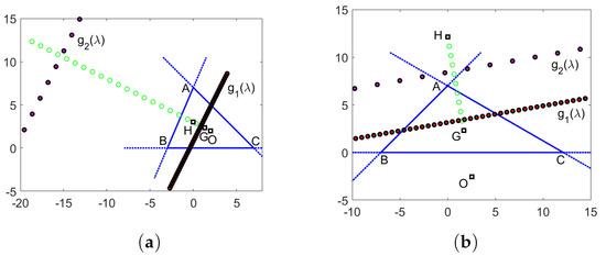
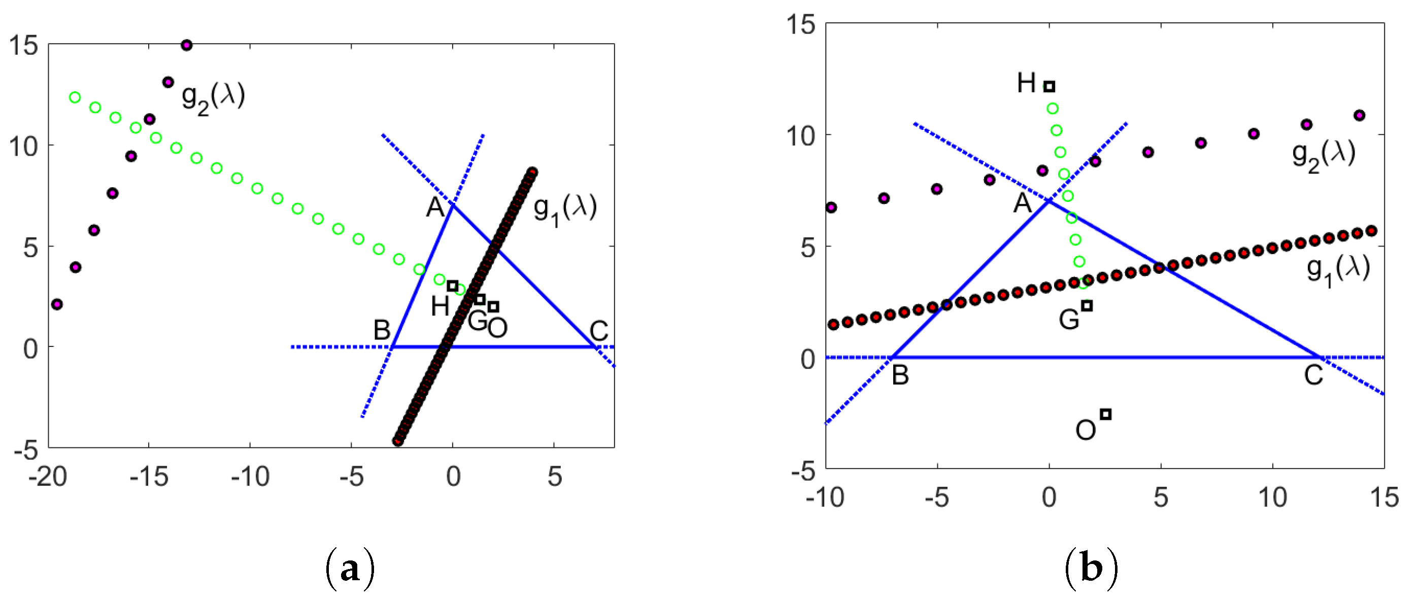
The two parallel lines of centroids $g_1\left(\lambda \right)$ and $g_2\left(\lambda \right)$ are shown in Figure 9.

Figure 9. First and second lines of centroids $g_1\left(\lambda \right)$ and $g_2\left(\lambda \right)$ given by (14) and (28), respectively, represented by red “x” symbols. (a) Acute triangle; (b) obtuse triangle. Also plotted are the centroid G, orthocenter H, and centre O of $\Delta ABC$.

The coordinates of this intersection point are given by

$$\begin{array}{c}\hfill Z_2=u_2·{\displaystyle \frac{\frac{\overline{v_3}}{\overline{u_2}}+\frac{v_3}{u_2}}{2}}=\Re \left({\displaystyle \frac{v_3}{u_2}}\right)·u_2.\end{array}$$

(30)

We have an analogous result to Theorem 1, for the second line of centroids.

Theorem 2. 

$\left(1\right)$ The second line of centroids $g_2\left(\lambda \right)$ is perpendicular to Euler’s line.

$\left(2\right)$ The intersection point between the line $g_2\left(\lambda \right)$, $\lambda \in \mathbb{R}$ and Euler’s line is

$$\begin{array}{c}\hfill Z_2=\Re \left({\displaystyle \frac{v_3}{u_2}}\right)·u_2.\end{array}$$

6. Alternative Approaches and Particular Examples

This section presents alternative proofs of the results.

6.1. Perpendicularity to Euler’s Line

For a direct proof of the result in Theorem 1 $\left(1\right)$, without using Lemma 1, it suffices to show that for ${\lambda }_1\ne {\lambda }_2$ we obtain

$$\begin{array}{c}\hfill {\displaystyle \frac{g_1\left({\lambda }_1\right)-g_1\left({\lambda }_2\right)}{a+b+c}}\in i·\mathbb{R}.\end{array}$$

Indeed, by formula (14), one obtains

$$\begin{array}{c}\hfill g_1\left({\lambda }_1\right)-g_1\left({\lambda }_2\right)=\left[k\left(1+\omega \right)\left(b-a\right)+\left(1+\overline{\omega }\right)\left(c-a\right)\right]·{\displaystyle \frac{{\lambda }_1-{\lambda }_2}{3}}.\end{array}$$

Furthermore, one can write

$$\begin{array}{cc}\hfill & k\left(1+\omega \right)\left(b-a\right)+\left(1+\overline{\omega }\right)\left(c-a\right)=\left(c-a\right)·\left[{\displaystyle \frac{\omega b-\overline{\omega }a}{\omega a-\overline{\omega }c}}\left(1+\omega \right)+\left(1+\overline{\omega }\right)\right]\hfill \\ \hfill & ={\displaystyle \frac{c-a}{\omega a-\overline{\omega }c}}·\left[\left(\omega b-\overline{\omega }a\right)\left(1+\omega \right)+\left(\omega a-\overline{\omega }c\right)\left(1+\overline{\omega }\right)\right]\hfill \\ \hfill & ={\displaystyle \frac{c-a}{\omega a-\overline{\omega }c}}·\left[\left(\omega -\overline{\omega }\right)a+\left(\omega +{\omega }^2\right)b+\left(-\overline{\omega }-{\overline{\omega }}^2\right)c\right]\hfill \\ \hfill & ={\displaystyle \frac{c-a}{\omega a-\overline{\omega }c}}·\left(a+b+c\right)·\sqrt{3}i,\hfill \end{array}$$

where for $\omega ={\displaystyle \frac{1}{2}}+{\displaystyle \frac{\sqrt{3}}{2}}i$, we use the identities

$$\omega -\overline{\omega }=\omega +{\omega }^2=-\overline{\omega }-{\overline{\omega }}^2=\sqrt{3}i.$$

Clearly, this shows that

$$\begin{array}{cc}\hfill {\displaystyle \frac{g_1\left({\lambda }_1\right)-g_1\left({\lambda }_2\right)}{a+b+c}}& ={\displaystyle \frac{{\lambda }_1-{\lambda }_2}{3}}·{\displaystyle \frac{c-a}{\omega a-\overline{\omega }c}}·\sqrt{3}i,\hfill \end{array}$$

which is purely imaginary since

$$\begin{array}{c}\hfill {\displaystyle \frac{\overline{c}-\overline{a}}{\overline{\omega }\overline{a}-\omega \overline{c}}}={\displaystyle \frac{\frac{1}{c}-\frac{1}{a}}{\frac{\overline{\omega }}{a}-\frac{\omega }{c}}}={\displaystyle \frac{c-a}{\omega a-\overline{\omega }c}}.\end{array}$$

This ends the proof. A proof based on trilinear coordinates was provided in [8].

Similarly, one can prove the result for the second line of centroids.

6.2. Intersection Points

From the condition $s\in \mathbb{R}$ (i.e., $s=\overline{s}$), we obtain

$$\begin{array}{c}\hfill s={\displaystyle \frac{g_1\left(\lambda \right)}{a+b+c}}={\displaystyle \frac{\overline{g_1\left(\lambda \right)}}{\overline{a}+\overline{b}+\overline{c}}}=\overline{s}.\end{array}$$

This condition reduces to

$$\begin{array}{c}\hfill {\displaystyle \frac{l\left(1+\omega \right)\left(b-a\right)+3a}{a+b+c}}-{\displaystyle \frac{l\left(1+\overline{\omega }\right)\left(\overline{b}-\overline{a}\right)+3\overline{a}}{\overline{a}+\overline{b}+\overline{c}}}=2l\sqrt{3}i·\lambda ,\end{array}$$

which gives (using that $l\in \mathbb{R}$)

$$\begin{array}{cc}\hfill & \left[l\left(1+\omega \right)\left(b-a\right)+3a\right]\left(\overline{a}+\overline{b}+\overline{c}\right)-\left[l\left(1+\overline{\omega }\right)\left(\overline{b}-\overline{a}\right)+3\overline{a}\right]\left(a+b+c\right)\hfill \\ \hfill & =2l\mid a+b+c{\mid }^2\sqrt{3}i·\lambda ,\hfill \end{array}$$

or

$$\begin{array}{c}\hfill 2·\lambda \sqrt{3}i={\displaystyle \frac{\left(1+\omega \right)\left(b-a\right)}{a+b+c}}-{\displaystyle \frac{\left(1+\overline{\omega }\right)\left(\overline{b}-\overline{a}\right)}{\overline{a}+\overline{b}+\overline{c}}}+{\displaystyle \frac{1}{l}}\left[{\displaystyle \frac{3a}{a+b+c}}-{\displaystyle \frac{3\overline{a}}{\overline{a}+\overline{b}+\overline{c}}}\right].\end{array}$$

By substituting $\lambda \sqrt{3}i$ in (20) and dividing by $a+b+c$, one obtains

$$\begin{array}{c}\hfill s=\Re \left[{\displaystyle \frac{l\left(1+\omega \right)\left(b-a\right)+3a}{3\left(a+b+c\right)}}\right],\end{array}$$

from where we deduce the following result.

Theorem 3. 

The intersection point between the first line of centroids $g_1\left(\lambda \right)$, $\lambda \in \mathbb{R}$ and Euler’s line of $\Delta ABC$ has the complex coordinates

$$\begin{array}{cc}\hfill Z& =\Re \left[{\displaystyle \frac{l\left(1+\omega \right)\left(b-a\right)+3a}{3\left(a+b+c\right)}}\right]·\left(a+b+c\right)\hfill \\ \hfill & =\Re \left[{\displaystyle \frac{\frac{a-c}{\omega a-\overline{\omega }c}\left(1+\omega \right)\left(b-a\right)+3a}{3\left(a+b+c\right)}}\right]·\left(a+b+c\right).\hfill \end{array}$$

Similarly, one can prove the coordinate of the intersection between the second line of centroids $g_2\left(\lambda \right)$, $\lambda \in \mathbb{R}$ and Euler’s line of $\Delta ABC$ as

$$\begin{array}{cc}\hfill Z_2& =\Re \left[{\displaystyle \frac{l_2\left(1+\overline{\omega }\right)\left(b-a\right)+3a}{3\left(a+b+c\right)}}\right]·\left(a+b+c\right)\hfill \\ \hfill & =\Re \left[{\displaystyle \frac{\frac{a-c}{\overline{\omega }a-\omega c}\left(1+\overline{\omega }\right)\left(b-a\right)+3a}{3\left(a+b+c\right)}}\right]·\left(a+b+c\right).\hfill \end{array}$$

6.3. Particular Examples and Formulas

In this section, we derive some particular formulas for the lines of centroids and their intersection with Euler’s line obtained for $a=0$. From (14), we obtain

$$\begin{array}{cc}\hfill g_1\left(\lambda \right)& ={\displaystyle \frac{m+n+p}{3}}=\left[k\left(1+\omega \right)b+\left(1+\overline{\omega }\right)c\right]·{\displaystyle \frac{\lambda }{3}}+{\displaystyle \frac{l\left(1+\omega \right)b}{3}},\hfill \end{array}$$

(31)

where by (9) and using $\omega -\overline{\omega }=\sqrt{3}i$, the values k and l are given by

$$\begin{array}{cc}\hfill k& ={\displaystyle \frac{\omega \left(b-c\right)\overline{c}-\overline{\omega }\left(\overline{b}-\overline{c}\right)c}{\omega b\left(\overline{b}-\overline{c}\right)-\overline{\omega }\overline{b}\left(b-c\right)}}={\displaystyle \frac{-{\left|c\right|}^2\sqrt{3}i+\left(\omega b\overline{c}-\overline{\omega b}c\right)}{{\left|b\right|}^2\sqrt{3}i-\left(\omega b\overline{c}-\overline{\omega b}c\right)}},\hfill \\ \hfill l& ={\displaystyle \frac{c\left(\overline{b}-\overline{c}\right)-\overline{c}\left(b-c\right)}{\omega b\left(\overline{b}-\overline{c}\right)-\overline{\omega }\overline{b}\left(b-c\right)}}={\displaystyle \frac{c\overline{b}-b\overline{c}}{{\left|b\right|}^2\sqrt{3}i-\left(\omega b\overline{c}-\overline{\omega b}c\right)}}.\hfill \end{array}$$

(32)

For the second line of centroids, we obtain

$$\begin{array}{cc}\hfill g_2\left(\lambda \right)& ={\displaystyle \frac{m_2+n+p_2}{3}}=\left[k_2\left(1+\overline{\omega }\right)b+\left(1+\omega \right)c\right]·{\displaystyle \frac{\lambda }{3}}+{\displaystyle \frac{l_2\left(1+\overline{\omega }\right)b}{3}},\hfill \end{array}$$

(33)

where by (13), the coefficients $k_2$ and $l_2$ are given by

$$\begin{array}{cc}\hfill k_2& ={\displaystyle \frac{\overline{\omega }\left(b-c\right)\overline{c}-\omega \left(\overline{b}-\overline{c}\right)c}{\overline{\omega }b\left(\overline{b}-\overline{c}\right)-\omega \overline{b}\left(b-c\right)}}={\displaystyle \frac{{\left|c\right|}^2\sqrt{3}i-\left(\omega c\overline{b}-\overline{\omega c}b\right)}{-{\left|b\right|}^2\sqrt{3}i+\left(\omega c\overline{b}-\overline{\omega c}b\right)}},\hfill \\ \hfill l_2& ={\displaystyle \frac{\left(\overline{b}-\overline{c}\right)c-\left(b-c\right)\overline{c}}{\overline{\omega }b\left(\overline{b}-\overline{c}\right)-\omega \overline{b}\left(b-c\right)}}={\displaystyle \frac{c\overline{b}-b\overline{c}}{-{\left|b\right|}^2\sqrt{3}i+\left(\omega c\overline{b}-\overline{\omega c}b\right)}}.\hfill \end{array}$$

(34)

We notice that these parametrizations are different from those in Section 5.

7. Conclusions

In this paper, we studied the equilateral triangles whose vertices are located on the support lines of a given arbitrary triangle. Using complex coordinates and a parametrization, we proved that the centers of these triangles are located on two lines, which are perpendicular to the Euler’s line of the given triangle, and we also computed the coordinates of these intersections.

It is interesting to investigate geometric properties related to triangles similar to a prototype whose vertices are located on the support lines of a given triangle.

References

- Apró, J. Triangles and Quadrilaterals Inscribed in Jordan Curves. Ph.D. Thesis, Eötvös Loránd University, Budapest, Hungary, 2023. [Google Scholar]
- Meyerson, M.D. Equilateral triangles and continuous curves. Fund. Math. 1980, 110, 1–9. [Google Scholar] [CrossRef]
- Nielsen, M.J. Triangles inscribed in simple closed curves. Geom. Dedicata 1992, 43, 291–297. [Google Scholar] [CrossRef]
- Gupta, A.; Rubinstein-Salzedo, S. Inscribed triangles of Jordan curves in . arXiv 2021, arXiv:2102.03953v1. [Google Scholar]
- Schwartz, R.E. Rectangles, curves, and Klein bottles. Bull. Amer. Math. Soc. 2022, 59, 1–17. [Google Scholar] [CrossRef]
- Stromquist, W. Inscribed squares and square-like quadrilaterals in closed curves. Mathematika 1989, 36, 187–197. [Google Scholar] [CrossRef]
- McCartin, B.J. Mysteries of the Equilateral Triangle; Hikari Ltd.: Rousse, Bulgaria, 2010. [Google Scholar]
- Capitán, F.J.G. Locus of centroids of similar inscribed triangles. Forum Geom. 2016, 16, 257–267. [Google Scholar]
- Kiss, N.S. Equal area triangles inscribed in a triangle. Int. J. Geom. 2016, 5, 19–30. [Google Scholar]
- Russell, R.A. Inscribed Equilateral Triangles. J. Classic Geom. 2015, 4, 1–6. [Google Scholar]
- Yaglom, I.M. Geometric Transformations II; Random House: London, UK, 1968; Translated from Russian. [Google Scholar]
- Andrica, D.; Bagdasar, O.; Marinescu, D.-Ş. Inscribed equilateral triangles in general triangles. Int. J. Geom. 2024, 13, 113–124. [Google Scholar]
- Čerin, Z. Configurations of inscribed equilateral triangles. J Geom. 2007, 87, 14–30. [Google Scholar] [CrossRef]
- Andreescu, T.; Andrica, D. Complex Numbers from A to …Z, 2nd ed.; Birkhäuser: Boston, MA, USA, 2014. [Google Scholar]
Disclaimer/Publisher’s Note: The statements, opinions and data contained in all publications are solely those of the individual author(s) and contributor(s) and not of MDPI and/or the editor(s). MDPI and/or the editor(s) disclaim responsibility for any injury to people or property resulting from any ideas, methods, instructions or products referred to in the content. |
© 2024 by the authors. Licensee MDPI, Basel, Switzerland. This article is an open access article distributed under the terms and conditions of the Creative Commons Attribution (CC BY) license (https://creativecommons.org/licenses/by/4.0/).