Homotopy Analysis Transform Method for a Singular Nonlinear Second-Order Hyperbolic Pseudo-Differential Equation

Abstract

In this study, we employed the homotopy analysis transform method (HATM) to derive an iterative scheme to numerically solve a singular second-order hyperbolic pseudo-differential equation. We evaluated the effectiveness of the derived scheme in solving both linear and nonlinear equations of similar nature through a series of illustrative examples. The stability of this scheme in handling the approximate solutions of these examples was studied graphically and numerically. A comparative analysis with existing methodologies from the literature was conducted to assess the performance of the proposed approach. Our findings demonstrate that the HATM-based method offers notable efficiency, accuracy, and ease of implementation when compared to the alternative technique considered in this study.

1. Introduction

Nonlinear partial differential equations serve as fundamental tools for describing a diverse array of phenomena across numerous scientific disciplines, including physics, biology, chemistry, economics, epidemiology, engineering, and beyond. Despite their ubiquity, exact solutions to the majority of these equations remain elusive. Consequently, various computational methodologies have been devised by researchers to address this challenge. Notable among these techniques are the Adomian decomposition method pioneered by G. Adomian [1,2,3,4], the variational iteration method introduced by J. He [5,6], the finite difference method developed by Crank–Nicolson in [7], the homotopy analysis method (HAM) proposed by Liao [8,9,10,11,12], the homotopy perturbation method advocated by J. He [13,14,15], and the differential transform method utilized by several researchers [16,17].

In recent years, a number of researchers have focused on investigating solutions to these partial differential equations through the integration of diverse techniques with the Laplace transform. Notable examples include the Laplace decomposition method detailed in references [18,19], the homotopy perturbation transform method explored in [20], and the introduction of the homotopy analysis transform method (HATM) as documented in [21]. Since then, the HATM has been widely implemented by many authors to solve various types of mathematical equations. For example, it was employed in [22] to solve a fractional equation modeling gas dynamics, and it was utilized in [23] to solve a fractional Fokker–Planck equation. In [24], it is applied to solve an integro-differential equation; in [25], the HATM was used to obtain exact solutions for fractional equations of type Korteweg–de Vries and Korteweg–de Vries–Burger’s; in [26], it was implemented to solve fractional Navier–Stokes equations; in [27], a modified version of the HATM was utilized to numerically solve a fractional-order smoking epidemic model; in [28], the HATM was employed to solve a nonlinear integro-differential equation; etc.

The goal of this study was to derive a numerical solution for a singular nonlinear second-order hyperbolic pseudo-differential equation based on the HATM. Moreover, the effectiveness of the proposed technique was explored through a set of illustrative example as well as a comparative analysis with existing methodologies in the literature. In particular, we employed the HATM to numerically solve the following pseudo-hyperbolic initial value problem:

$$\frac{{\partial }^2}{\partial t^2}\mathcal{U}(x,t)-\frac{\alpha }{x}\frac{\partial }{\partial x}\left(x\frac{\partial \mathcal{U}}{\partial x}\right)-\frac{\beta }{x}\frac{{\partial }^2}{\partial x\partial t}\left(x\frac{\partial \mathcal{U}}{\partial x}\right)-\gamma x^2\frac{\partial }{\partial x}\left(\mathcal{U}\frac{\partial \mathcal{U}}{\partial x}\right)+\lambda F\left(\mathcal{U}\right)=\mathcal{G}(x,t),$$

(1)

subject to the constraints

$$\mathcal{U}(x,0)=g_1\left(x\right),\frac{\partial }{\partial x}\mathcal{U}(x,0)=g_2\left(x\right),$$

where $\alpha$, $\beta$, $\gamma$, and $\lambda$ are constants, and $\mathcal{F}, \mathcal{G}, g_1,$ and $g_2$ are known functions.

In fact, at $\beta =\gamma =\lambda =0$, Equation (1) reduces to a singular one-dimensional wave equation, and at $\alpha =\gamma =\lambda =0$, it reduces to a singular one-dimensional pseudo-wave equation.

The nonlinear singular one-dimensional pseudo-hyperbolic equation is a type of PDE that involves mixed partial derivatives in space and time, and it exhibits both hyperbolic and singular characteristics. In general, these equations are often used to model complex physical phenomena. In our model, the equation describes how waves propagate, attenuate, and interact in a medium with radial symmetry, such as sound waves in a cylindrical duct or stress waves in a cylindrical rod. The nonlinear terms in the equation represent complex interactions, like nonlinear elastic responses or external forces acting on the medium. These nonlinear terms can lead to complex behaviors such as wave steepening, shock formation, or solitons. They often represent interactions within the medium or external forces that depend on the wave’s state. More precisely, the equation models a radial wave propagation in an elastic medium, where the Bessel operator reflects the radial nature of wave propagation.

To achieve our goal, we need the Laplace transform for a second-order partial derivative of the function $\mathcal{U}$ with respect to t which is given by

$$L\left[\frac{{\partial }^2}{\partial t^2}\mathcal{U}(x,t)\right]=s^2\mathcal{U}(x,s)-s \mathcal{U}(x,0)-\frac{\partial }{\partial t}\mathcal{U}(x,0).$$

(2)

Let us mention that linear and nonlinear versions of Equation (1) were considered in [29], where a combination of the double Laplace transform and the Adomian decomposition method was applied to solve these versions.

The rest of this paper is organized as follows. In Section 2, we provide the basic outlines of the HATM. In Section 3, the HATM is employed to derive the numerical method for solving model (1). Section 4 is devoted to the application of the derived iterative scheme to a set of test examples to evaluate its efficiency. Finally, in Section 5, we comment on our findings and conclusions.

2. Basic Outline of HATM

The homotopy analysis transform method was first introduced in [21]. It is an elegant combination of the Laplace transform method and the homotopy analysis method. Its implementation does not require discretization or any other restrictive assumptions, which avoid round-off errors that may affect the reach of a closed-form solution of the problem. Moreover, it does not require decomposing the nonlinear terms in the equation under consideration, which usually leads to tedious algebraic work. Additionally, for some strongly nonlinear problems other techniques may fail to produce a convergent series solution, while the existence of the parameter ℏ in theh HATM can be used to adjust and control the convergence region to ensure the convergence of a series solution for such problems. This reveals that the HATM is a very effective and accurate method in handling the solution of various nonlinear types of partial differential equations. Thus, our motivation for this work was to determine a numerical solution for the singular problem (1) based on the HATM that is easy to implement and does not require any restrictive assumptions needed for the implementation of the aforementioned methods. To formulate the basic outlines of the HATM, we consider a general partial differential equation as follows:

$${\partial }_t^2\mathcal{U}(x,t)+\mathcal{R}\mathcal{U}(x,t)+\mathcal{N}\mathcal{U}(x,t)=g(x,t),$$

(3)

subject to the initial conditions

$$\mathcal{U}(x,0)=f_1\left(x\right) \mathrm{and} {\mathcal{U}}_t(x,0)=f_2\left(x\right),$$

where $\mathcal{R}$ represents a linear differential operator, $\mathcal{N}$ represents a nonlinear differential operator, and $g, f_1$, and $f_2$ are known functions.

Taking the Laplace transform L for both sides of Equation (3) implies that

$$s^{2}L\left\{\mathcal{U}(x,t)\right\}-s\mathcal{U}(x,0)-{\mathcal{U}}_t(x,0)+L\left\{\mathcal{R}\mathcal{U}(x,t)+\mathcal{N}\mathcal{U}(x,t)\right\}=L\left\{g(x,t)\right\},$$

that is,

$$L\left\{\mathcal{U}(x,t)\right\}-\frac{1}{s}\mathcal{U}(x,0)-\frac{1}{s^2}{\mathcal{U}}_t(x,0)+\frac{1}{s^2}L\left\{\mathcal{R}\mathcal{U}(x,t)+\mathcal{N}\mathcal{U}(x,t)-g(x,t)\right\}=0.$$

Thus, according to the theory of the HAM [8], we can define an operator $\mathsf{N}$ as follows:

$$\begin{array}{ccc}\mathsf{N}\left[\varphi \right(x,t;q\left)\right]\hfill & =\hfill & L\left\{\varphi (x,t;q)\right\}-\frac{1}{s}\varphi (x,0;q)-\frac{1}{s^2}{\varphi }_t(x,0;q)+\frac{1}{s^2}L\{\mathcal{R}\varphi (x,t;q)\hfill \\ \hfill & \hfill & +\mathcal{N}\varphi (x,t;q)-g(x,t)\},\hfill \end{array}$$

where $q\in [0,1],$ and $\varphi$ is a real-valued function in $x,t$, and q.

Then, we can define the zeroth-order deformation equation as follows:

$$(1-q)L\left[\varphi (x,t;q)-{\mathcal{U}}_0(x,t)\right]=q\hslash \mathsf{N}\left[\varphi (x,t;q)\right],$$

(4)

where $q\in [0,1]$ is an embedding parameter; L is the Laplace transform operator; ${\mathcal{U}}_0(x,t)$ is an initial approximation of the exact solution $\mathcal{U}(x,t)$; $\varphi (x,t;q)$ is an unknown function of $x, t,$ and q; and ℏ is a nonzero auxiliary parameter, which plays a fundamental role in the convergence of the series solution.

It follows from Equation (4) that $\varphi (x,t;0)={\mathcal{U}}_0(x,t)$ at $q=0$ and $\varphi (x,t;1)=\mathcal{U}(x,t)$ at $q=1$. Thus, as q moves continuously from 0 to 1, the function $\varphi (x,t;q)$ deforms from the initial guess ${\mathcal{U}}_0(x,t)$ toward the exact solution $\mathcal{U}(x,t)$.

Next, the Taylor series expansion of $\varphi (x,t;q)$ in powers of q yields

$$\varphi (x,t;q)={\mathcal{U}}_0(x,t)+\sum _{i=1}^{\infty }{\mathcal{U}}_i(x,t) q^i,$$

(5)

where

$${\mathcal{U}}_i(x,t)={\left.\frac{1}{i!}\frac{{\partial }^i\varphi (x,t;q)}{\partial q^i}\right|}_{q=0}.$$

As Liao pointed out in [11], if the initial guess ${\mathcal{U}}_0(x,t)$ and the parameter ℏ are chosen properly, then power series (5) will converge at $q=1$ to a solution of the considered partial differential equation, and this solution is expressed in series form as follows:

$$\mathcal{U}(x,t)={\mathcal{U}}_0(x,t)+\sum _{i=1}^{\infty }{q}^i{\mathcal{U}}_i(x,t).$$

In fact, the success of the convergence of the series solution in the HATM depends on three elements, namely, the choice of the operator to be inverted, the value of the parameter ℏ, and the initial guess. The choice of the suitable operator takes into account that the operator is easily inverted. The existence of the parameter ℏ distinguishes the HATM from other semi-analytical methods, as its occurrence in the series solution enables one to adjust the convergence interval as required. But in the absence of easy theoretical techniques that can be implemented to determine its value, an alternative graphical technique based on the h-curve resulting from the plots of the approximate truncated series solutions is used to determine a range of values for this parameter, usually the interval on which the curve is almost horizontal. Finally, the choice of the initial guess depends on the operator to be inverted. It can be chosen from the initial or boundary conditions in the problem according to the inverted operator, and it should satisfy the differential equation under consideration.

Now, differentiating Equation (4) k times with respect to q, setting $q=0$, and dividing the result by $k!$ produce the following kth-order deformation equation:

$$L\left\{{\mathcal{U}}_k(x,t)-{\chi }_k{\mathcal{U}}_{k-1}(x,t)\right\}=\hslash \mathsf{R}\left({\overrightarrow{\mathcal{U}}}_{k-1}\right),$$

(6)

where

$$\overrightarrow{{\mathcal{U}}_k}(x,t)=[{\mathcal{U}}_0(x,t),{\mathcal{U}}_1(x,t),\dots ,{\mathcal{U}}_k(x,t)],$$

and

$$\mathsf{R}\left({\overrightarrow{\mathcal{U}}}_{k-1}\right)={\left.\frac{1}{(k-1)!}\left\{\frac{{\partial }^{k-1}}{\partial q^{k-1}}\mathsf{N}\left[\varphi (x,t;q)\right]\right\}\right|}_{q=0}.$$

Finally, taking the inverse Laplace transform for both sides of Equation (6) implies that the components ${\mathcal{U}}_k(x,t), k=1,2,\dots ,$ can be determined by applying the following iterative formula:

$${\mathcal{U}}_k(x,t)={\chi }_k{\mathcal{U}}_{k-1}(x,t)+\hslash L^{-1}\left[\mathsf{R}\left({\overrightarrow{\mathcal{U}}}_{k-1}\right)\right],$$

where

$${\chi }_k=\left\{\begin{array}{cc}0,\hfill & k\le 1,\hfill \\ 1,\hfill & k > 1.\hfill \end{array}\right.$$

Let us mention that the accuracy of the numerical solution will be improved as the number of terms in the truncated series solution is increased. On the other hand, the computational process can be terminated when either of the computed components lead to the closed-form solution or the terminated series solution provide the required accuracy of the numerical solution.

3. Application of the Method

To explore the applicability and efficiency of the HATM for solving problem (1) subject to initial conditions

$$\mathcal{U}(x,0)=g_1\left(x\right),\frac{\partial }{\partial x}\mathcal{U}(x,0)=g_2\left(x\right),$$

where $g_1,$ and $g_2$ are known functions, we apply the Laplace transform to both sides of this equation to obtain

$$L\left[\mathcal{U}(x,t)\right]-\frac{1}{s} g_1\left(x\right)-\frac{1}{s^2} g_2\left(x\right)-\frac{1}{s^2} L\left[\frac{\alpha }{x}{\left(x{\mathcal{U}}_x\right)}_x+\frac{\beta }{x}{\left(x{\mathcal{U}}_x\right)}_{tx}+\gamma x^2{\left(\mathcal{U}{\mathcal{U}}_x\right)}_x-\lambda F\left(\mathcal{U}\right)+\mathcal{G}(x,t)\right]=0.$$

Thus, we define an operator $\mathcal{N}\left[\varphi \right(x,t;q\left)\right]$ as follows:

$$\begin{array}{ccc}\mathsf{N}\left[\varphi \right(x,t;q\left)\right]\hfill & =\hfill & L\left\{\varphi (x,t;q)\right\}-\frac{1}{s}{g}_1\left(x\right)-\frac{1}{s^2}{g}_2\left(x\right)-\frac{1}{s^2}L[\frac{\alpha }{x}{\left(x{\varphi }_x(x,t;q)\right)}_x+\frac{\beta }{x}{\left(x{\varphi }_x(x,t;q)\right)}_{tx}\hfill \\ \hfill & \hfill & +\gamma x^2{\left(\varphi (x,t;q){\varphi }_x(x,t;q)\right)}_x-\lambda F\left(\varphi (x,t;q)\right)+\mathcal{G}(x,t)].\hfill \end{array}$$

Therefore, the kth-order deformation equation can be defined as follows:

$$L[{\mathcal{U}}_k(x,t)-{\chi }_k{\mathcal{U}}_{k-1}(x,t)]=\hslash \mathsf{R}\left({\overrightarrow{\mathcal{U}}}_{k-1}\right),$$

where

$$\begin{array}{ccc}\mathsf{R}\left({\overrightarrow{\mathcal{U}}}_{k-1}\right)\hfill & =\hfill & L\left\{{\mathcal{U}}_{k-1}(x,t)\right\}-\left(1-{\chi }_k\right)\left(\frac{1}{s}{g}_1\left(x\right)+\frac{1}{s^2}{g}_2\left(x\right)\right)-\frac{1}{s^2}L[\frac{\alpha }{x}\frac{\partial }{\partial x}\left(x\frac{\partial }{\partial x}{\mathcal{U}}_{k-1}(x,t)\right)\hfill \\ \hfill & \hfill & +{\displaystyle \frac{\beta }{x}\frac{{\partial }^2}{\partial x\partial t}(x\frac{\partial }{\partial x}{\mathcal{U}}_{k-1}(x,t))+\gamma x^2\frac{\partial }{\partial x}({\mathcal{U}}_{k-1}(x,t)\frac{\partial }{\partial x}{\mathcal{U}}_{k-1}(x,t))}\hfill \\ \hfill & \hfill & -\lambda F\left({\mathcal{U}}_{k-1}(x,t)\right)+\left(1-{\chi }_k\right)\mathcal{G}(x,t)].\hfill \end{array}$$

Hence, the components of the series solution can be computed recursively from the iterative formula

$${\mathcal{U}}_k(x,t)={\chi }_k{\mathcal{U}}_{k-1}(x,t)+\hslash L^{-1}\left[\mathsf{R}\left({\overrightarrow{\mathcal{U}}}_{k-1}\right)\right], k=1,2,\dots ,$$

(7)

and the solution is given by

$$\mathcal{U}(x,t)={\mathcal{U}}_0(x,t)+\sum _{k=1}^{\infty } {\mathcal{U}}_k(x,t).$$

4. Numerical Results

In this section, we test the efficiency and accuracy of scheme (7) in handling the numerical solutions for problems of type (1). It is notable to mention that all computations in this section were conducted using the software Mathematica 8.04.0., and all the numerical results in the tables were computed using the default machine precision and accuracy of 17 significant digits rounded to 6 significant digits. Now, we apply this scheme to the following set of examples.

Example 1.

Consider the singular linear partial differential equation

$$\frac{{\partial }^2}{\partial t^2}\mathcal{U}(x,t)-\frac{1}{x}\frac{\partial }{\partial x}(x\frac{\partial \mathcal{U}}{\partial x})-\frac{1}{x}\frac{{\partial }^2}{\partial x\partial t}(x\frac{\partial \mathcal{U}}{\partial x})=\mathcal{G}(x,t),$$

subject to the following initial constraints:

$$\mathcal{U}(x,0)=0 and\frac{\partial \mathcal{U}}{\partial t}(x,0)=x^2,$$

where $\mathcal{G}(x,t)=-x^{2}sint-4sint-4cost$.

Solution.

Let ${\mathcal{U}}_0(x,t)=\mathcal{U}(x,0)=x^2$. Then, in view of (7), we obtain

$$\begin{array}{ccc}{\mathcal{U}}_1(x,t)\hfill & =\hfill & {\chi }_1{\mathcal{U}}_0(x,t)+\hslash L^{-1}\left[\mathsf{R}\left({\overrightarrow{\mathcal{U}}}_0\right)\right]\hfill \\ \hfill & =\hfill & \hslash L^{-1}\left[\mathsf{R}\left({\overrightarrow{\mathcal{U}}}_0\right)\right]\hfill \\ \hfill & =\hfill & {\displaystyle -\hslash \left(-4(1+t)+4cost+\left(4+x^2\right)sint\right)},\hfill \end{array}$$

$$\begin{array}{ccc}{\mathcal{U}}_2(x,t)\hfill & =\hfill & {\chi }_2{\mathcal{U}}_1(x,t)+\hslash L^{-1}\left[\mathsf{R}\left({\overrightarrow{\mathcal{U}}}_1\right)\right]\hfill \\ \hfill & =\hfill & {\mathcal{U}}_1(x,t)+\hslash L^{-1}\left[\mathsf{R}\left({\overrightarrow{\mathcal{U}}}_1\right)\right]\hfill \\ \hfill & =\hfill & {\displaystyle -\hslash \left(-4(1+2\hslash )(1+t)+(4+8\hslash )cost+\left(4+x^2+\hslash \left(8+x^2\right)\right)sint\right)},\hfill \end{array}$$

$$\begin{array}{ccc}{\mathcal{U}}_3(x,t)\hfill & =\hfill & {\chi }_3{\mathcal{U}}_2(x,t)+\hslash L^{-1}\left[\mathsf{R}\left({\overrightarrow{\mathcal{U}}}_2\right)\right]\hfill \\ \hfill & =\hfill & {\mathcal{U}}_2(x,t)+\hslash L^{-1}\left[\mathsf{R}\left({\overrightarrow{\mathcal{U}}}_2\right)\right]\hfill \\ \hfill & =\hfill & {\displaystyle -\hslash (1+\hslash )\left(-4(1+3\hslash )(1+t)+4(1+3\hslash )cost+\left(4+x^2+\hslash \left(12+x^2\right)\right)sint\right)}.\hfill \end{array}$$

⋯

Thus, the series solution is given by

$$\begin{array}{ccc}\mathcal{U}(x,t)\hfill & =\hfill & {\mathcal{U}}_0(x,t)+{\mathcal{U}}_1(x,t)+{\mathcal{U}}_3(x,t)+\dots \hfill \\ \hfill & =\hfill & 12\hslash {(1+\hslash )}^2\left(1+t-cost\right)-\hslash \left(3\left(4+x^2\right)+3\hslash \left(8+x^2\right)+{\hslash }^2\left(12+x^2\right)\right)sint+\dots .\hfill \end{array}$$

(8)

It is noticed that at $\hslash =-1$, the components of the series solution (8) are reduced to

$${\mathcal{U}}_1(x,t)=-4(1+t)+4cost+\left(4+x^2\right)sint.$$

$${\mathcal{U}}_2(x,t)=-4(-1-t+cost+sint).$$

$${\mathcal{U}}_3(x,t)=0.$$

Continuing in this manner, we obtain ${\mathcal{U}}_j(x,t)=0$ for all $j\ge 3$. Hence, the series solution (8) reduces to

$$\begin{array}{ccc}\mathcal{U}(x,t)\hfill & =\hfill & {\mathcal{U}}_0(x,t)+{\mathcal{U}}_1(x,t)+{\mathcal{U}}_3(x,t)+\dots \hfill \\ \hfill & =\hfill & x^{2}sint,\hfill \end{array}$$

which is the exact solution for this equation given in [29].

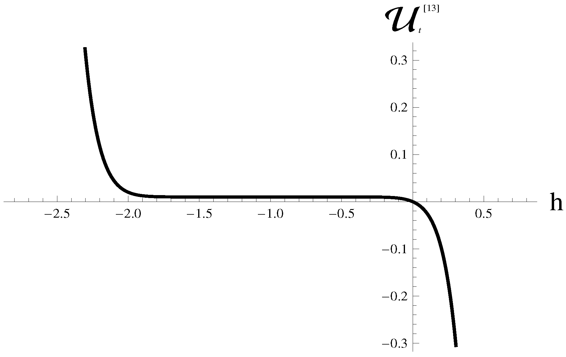
Figure 1 shows the h-curve corresponding to the 13th-order series solution. This figure shows that the values of ℏ that lead to the convergence of the series solution (9) should be selected from the range $-1.9<\hslash <-0.2$.

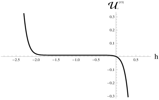
Figure 1. The ℏ-curve corresponding to the 13th-order truncated series solution at $x=0.1$.

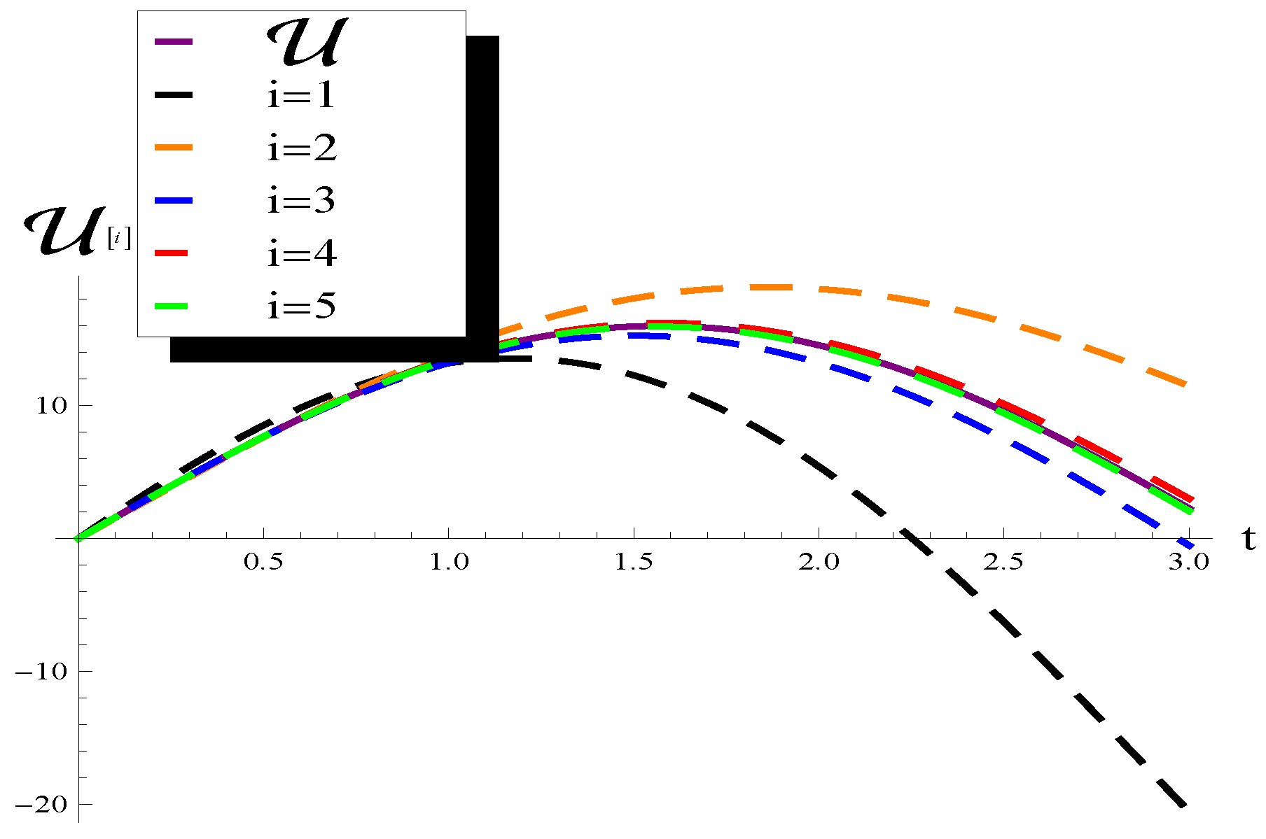
Figure 2 shows plots of the truncated series solutions for Example 1 with a different number of terms at $x=4$ and $\hslash =-1.2$. This figure shows the rapid convergence of these approximate solutions toward the exact solution. It illustrates that the curves of the truncated series solutions are getting closer to the exact solution as the number of terms in the truncated series solution is increased.

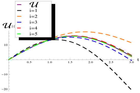
Figure 2. Truncated series solution ${\mathcal{U}}^{\left[i\right]}(x,t)$ with various values of i for Example 1.

Table 1 and Table 2 show the absolute error $E{r}^{\left[i\right]}=|\mathcal{U}(x,t)-{\mathcal{U}}^{\left[i\right]}(x,t)|$ resulting from taking the difference between the exact solution and the approximate solution of several orders of Example 1 at different values of $\hslash ,$t, and x. These data illustrate the rapid convergence of the approximate solution just after a few terms. Moreover, it appears from an error analysis of these tables that the convergence of the approximate solutions is more rapid at $\hslash =-1$ than at the other values of ℏ in the interval of convergence.

Table 1. Absolute error at $x=0.1$ and different values of ℏ, i, and t.

ℏ	$\mathit{i}$	t
		0.1	0.5	1	2
		${\mathit{Er}}^{\left[\mathit{i}\right]}$	${\mathit{Er}}^{\left[\mathit{i}\right]}$	${\mathit{Er}}^{\left[\mathit{i}\right]}$	${\mathit{Er}}^{\left[\mathit{i}\right]}$
−0.9	1	$0.0186845$	$0.515250$	$2.22646$	$9.02557$
	5	$9.30234\times {10}^{-6}$	$2.57433\times {10}^{-4}$	$1.11289\times {10}^{-3}$	$4.51242\times {10}^{-3}$
	10	$1.85947\times {10}^{-10}$	$5.14819\times {10}^{-9}$	$2.2257\times {10}^{-8}$	$9.02475\times {10}^{-8}$
	15	$2.77642\times {10}^{-15}$	$7.6621\times {10}^{-14}$	$3.34507\times {10}^{-13}$	$1.35459\times {10}^{-12}$
−1	1	$0.0206497$	$0.571968$	$2.47291$	$10.0274$
	5	$8.45678\times {10}^{-18}$	$1.96024\times {10}^{-16}$	$1.17267\times {10}^{-15}$	$1.12930\times {10}^{-15}$
	10	$8.45678\times {10}^{-18}$	$1.96024\times {10}^{-16}$	$1.17267\times {10}^{-15}$	$1.12930\times {10}^{-15}$
	15	$8.45678\times {10}^{-18}$	$1.96024\times {10}^{-16}$	$1.17267\times {10}^{-15}$	$1.12930\times {10}^{-15}$
−1.1	1	$0.0226148$	$0.628685$	$2.71936$	$11.0292$
	5	$1.13473\times {10}^{-5}$	$3.14534\times {10}^{-4}$	$1.36001\times {10}^{-3}$	$5.51498\times {10}^{-3}$
	10	$2.27046\times {10}^{-10}$	$6.29116\times {10}^{-9}$	$2.72011\times {10}^{-8}$	$1.10300\times {10}^{-7}$
	15	$3.57505\times {10}^{-15}$	$9.37245\times {10}^{-14}$	$4.08033\times {10}^{-13}$	$1.65583\times {10}^{-12}$

Table 2. Absolute error at $x=5$ and different values of ℏ, i, and t.

ℏ	$\mathit{i}$	t
		0.1	0.5	1	2
		${\mathit{Er}}^{\left[\mathit{i}\right]}$	${\mathit{Er}}^{\left[\mathit{i}\right]}$	${\mathit{Er}}^{\left[\mathit{i}\right]}$	${\mathit{Er}}^{\left[\mathit{i}\right]}$
−0.9	1	$0.268168$	$1.71333$	$4.32929$	$11.2979$
	5	$3.42507\times {10}^{-5}$	$3.77242\times {10}^{-4}$	$1.32318\times {10}^{-3}$	$4.73965\times {10}^{-3}$
	10	$4.35430\times {10}^{-10}$	$6.34627\times {10}^{-9}$	$2.43598\times {10}^{-8}$	$9.25198\times {10}^{-8}$
	15	$5.32907\times {10}^{-15}$	$9.05942\times {10}^{-14}$	$3.51719\times {10}^{-13}$	$1.37490\times {10}^{-12}$
−1	1	$0.0206497$	$0.571968$	$2.47291$	$10.0274$
	5	$4.44089\times {10}^{-16}$	$3.55271\times {10}^{-15}$	$3.55271\times {10}^{-15}$	$3.55271\times {10}^{-15}$
	10	$4.44089\times {10}^{-16}$	$3.55271\times {10}^{-15}$	$3.55271\times {10}^{-15}$	$3.55271\times {10}^{-15}$
	15	$4.44089\times {10}^{-16}$	$3.55271\times {10}^{-15}$	$3.55271\times {10}^{-15}$	$3.55271\times {10}^{-15}$
−1.1	1	$0.226869$	$0.569399$	$0.616520$	$8.75689$
	5	$1.36010\times {10}^{-5}$	$1.94726\times {10}^{-4}$	$1.14973\times {10}^{-3}$	$5.28774\times {10}^{-3}$
	10	$2.24376\times {10}^{-11}$	$5.09308\times {10}^{-9}$	$2.50983\times {10}^{-8}$	$1.08028\times {10}^{-7}$
	15	$1.33227\times {10}^{-15}$	$8.17124\times {10}^{-14}$	$3.87246\times {10}^{-13}$	$1.63780\times {10}^{-12}$

Example 2.

Consider the singular nonlinear partial differential equation

$$\frac{{\partial }^2}{\partial t^2}\mathcal{U}(x,t)-\frac{1}{x}\frac{\partial }{\partial x}(x\frac{\partial \mathcal{U}}{\partial x})-\frac{1}{x}\frac{{\partial }^2}{\partial x\partial t}(x\frac{\partial \mathcal{U}}{\partial x})-\frac{x}{2} \mathcal{U}\frac{\partial \mathcal{U}}{\partial x}+{\mathcal{U}}^2=x^2 e^{-t},$$

subject to the following initial conditions:

$$\mathcal{U}(x,0)=x^2 and\frac{\partial \mathcal{U}}{\partial t}(x,0)=-x^2.$$

Solution.

Let ${\mathcal{U}}_0(x,t)=x^2 e^{-t}$. Then, in view of (7), we obtain

$$\begin{array}{ccc}{\mathcal{U}}_1(x,t)\hfill & =\hfill & {\chi }_1{\mathcal{U}}_0(x,t)+\hslash L^{-1}\left[\mathsf{R}\left({\overrightarrow{\mathcal{U}}}_0\right)\right]\hfill \\ \hfill & =\hfill & \hslash L^{-1}\left[\mathsf{R}\left({\overrightarrow{\mathcal{U}}}_0\right)\right]\hfill \\ \hfill & =\hfill & 0,\hfill \end{array}$$

$$\begin{array}{ccc}{\mathcal{U}}_2(x,t)\hfill & =\hfill & {\chi }_2{\mathcal{U}}_1(x,t)+\hslash L^{-1}\left[\mathsf{R}\left({\overrightarrow{\mathcal{U}}}_1\right)\right]\hfill \\ \hfill & =\hfill & {\mathcal{U}}_1(x,t)+\hslash L^{-1}\left[\mathsf{R}\left({\overrightarrow{\mathcal{U}}}_1\right)\right]\hfill \\ \hfill & =\hfill & 0,\hfill \end{array}$$

Continuing in this manner, we obtain ${\mathcal{U}}_j(x,t)=0$ for all $j\ge 1$. Thus, the series solution is given by

$$\begin{array}{ccc}\mathcal{U}(x,t)\hfill & =\hfill & {\mathcal{U}}_0(x,t)+{\mathcal{U}}_1(x,t)+{\mathcal{U}}_3(x,t)+\dots \hfill \\ \hfill & =\hfill & x^2 e^{-t},\hfill \end{array}$$

which is the exact solution for this equation presented in [29], without using Adomain polynomials.

Example 3.

Consider the singular nonlinear partial differential equation

$$\frac{{\partial }^2}{\partial t^2}\mathcal{U}(x,t)-\frac{1}{x}\frac{\partial }{\partial x}(x\frac{\partial \mathcal{U}}{\partial x})-\frac{1}{x}\frac{{\partial }^2}{\partial x\partial t}(x\frac{\partial \mathcal{U}}{\partial x})-x^2 \frac{\partial }{\partial x}\left(\mathcal{U}\frac{\partial \mathcal{U}}{\partial x}\right)=lnx-t-1,$$

subject to the following initial conditions:

$$\mathcal{U}(x,0)=-lnx and\frac{\partial \mathcal{U}}{\partial t}(x,0)=1.$$

Solution.

Let ${\mathcal{U}}_0(x,t)=\mathcal{U}(x,0)=-lnx$. Then, in view of (7), we obtain

$${\mathcal{U}}_1(x,t)=\frac{1}{6}\hslash t\left(-6+t^2\right),$$

$${\mathcal{U}}_2(x,t)=\frac{1}{6}\hslash t\left(-6+t^2\right)-\frac{1}{120}{\hslash }^{2}t\left(120-40t^2+t^4\right),$$

$${\mathcal{U}}_3(x,t)=\frac{1}{6}\hslash t\left(-6+t^2\right)-\frac{1}{60}{\hslash }^{2}t\left(120-40t^2+t^4\right)+\frac{{\hslash }^{3}t\left(-5040+2520t^2-126t^4+t^6\right)}{5040},$$

Thus, the series solution is given by

$$\begin{array}{ccc}\mathcal{U}(x,t)\hfill & =\hfill & {\mathcal{U}}_0(x,t)+{\mathcal{U}}_1(x,t)+{\mathcal{U}}_3(x,t)+\dots \hfill \\ \hfill & =\hfill & -lnx+\frac{\hslash t}{2}\left(-6+t^2\right)-\frac{{\hslash }^{2}t}{40}\left(120-40t^2+t^4\right)+\frac{{\hslash }^{3}t}{5040}\left(-5040+2520t^2-126t^4+t^6\right)+\dots .\hfill \end{array}$$

(9)

In fact, at $\hslash =-1$, the components of the series solution (9) are reduced to

$${\mathcal{U}}_1(x,t)=t\left(1-\frac{t^2}{6}\right),$$

$${\mathcal{U}}_2(x,t)=\frac{1}{120}{t}^3\left(20-t^2\right),$$

$${\mathcal{U}}_3(x,t)=\frac{t^5\left(42-t^2\right)}{5040},$$

In general, we have

$${\mathcal{U}}_j(x,t)=\frac{t^{2j-1}}{(2j+1)!}\left[2j(2j+1)-t^2\right].$$

Hence, series solution (9) reduces to

$$\mathcal{U}(x,t)=-lnx+\sum _{j=1}^{\infty }\frac{t^{2j-1}}{(2j+1)!}\left[2j(2j+1)-t^2\right].$$

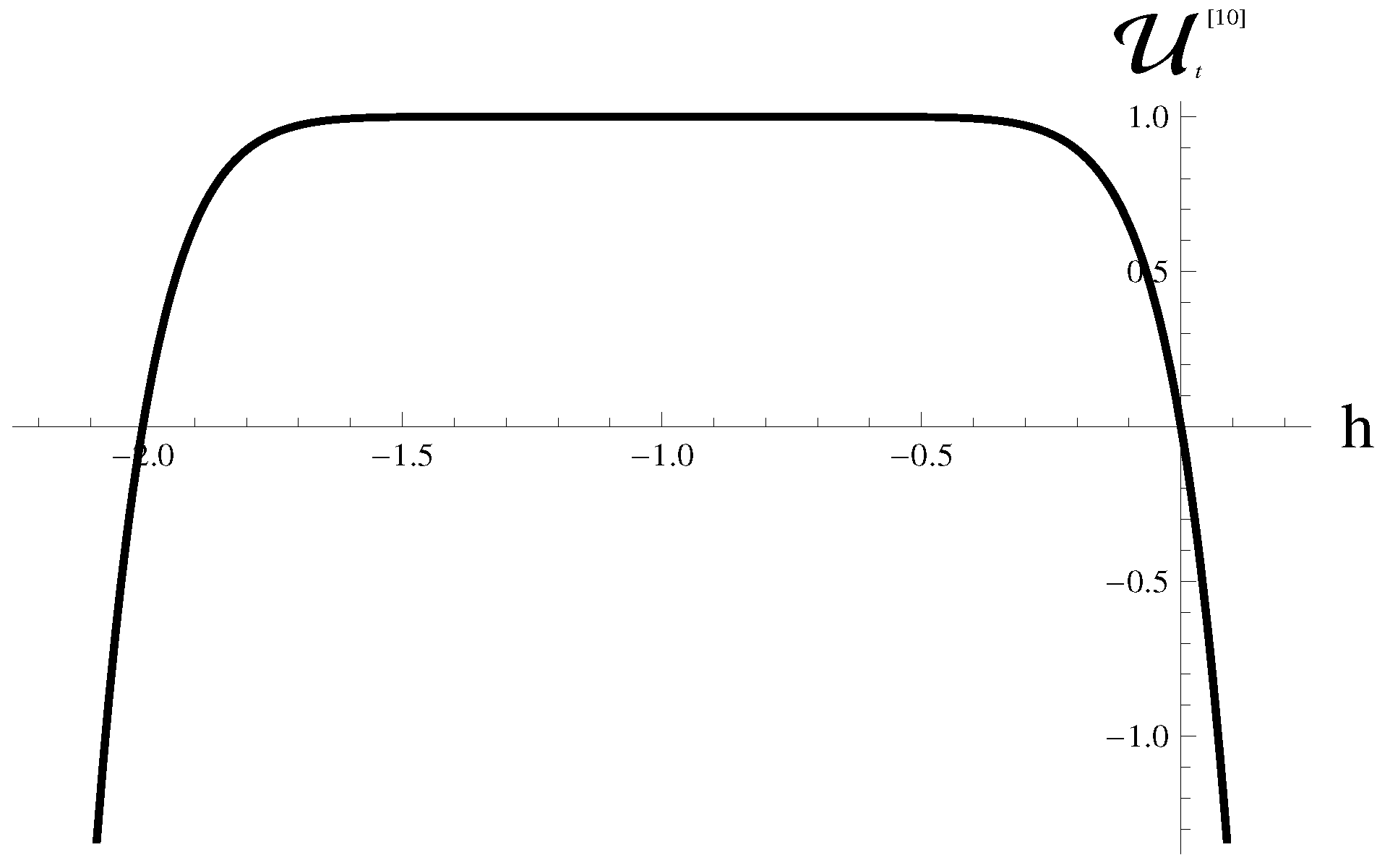
Figure 3 shows the h-curve corresponding to the 10th-order series solution. This figure shows that the values of ℏ that lead to the convergence of series solution (9) should be selected from the interval $-1.7<\hslash <-0.4$.

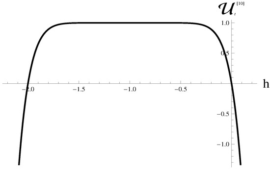
Figure 3. The ℏ-curve corresponding to the 10^th-order truncated series solution at $x=0.1$.

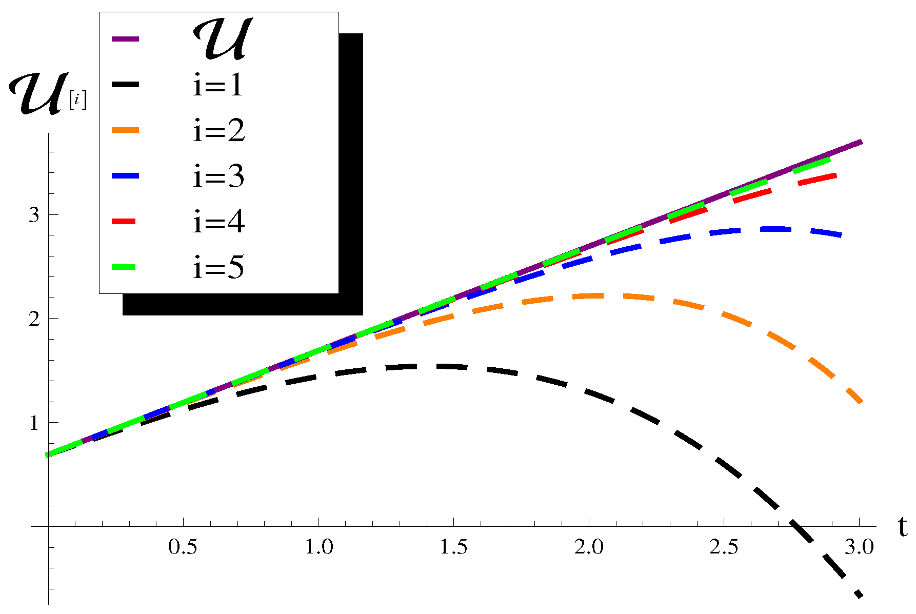
Figure 4 shows plots of the truncated series solutions for Example 3 with a different number of terms at $x=0.1$ and $\hslash =-0.9$. This figure shows the rapid convergence of these approximate solutions toward the exact solution. It illustrates that the curves of the truncated series solutions are getting closer to the exact solution as the number of terms in the truncated series solution is increased.

Figure 4. Truncated series solution ${\mathcal{U}}^{\left[i\right]}(x,t)$ with various values of i for Example 3.

The exact solution of Example 3 is $\mathcal{U}(x,t)=tlnx$. Table 3 and Table 4 show the absolute error $E{r}^{\left[i\right]}=|\mathcal{U}(x,t)-{\mathcal{U}}^{\left[i\right]}(x,t)|$ resulting from taking the difference between the exact solution and the approximate solution of several orders at different values of $\hslash ,$t, and x. These data demonstrate the rapid convergence of the approximate solution just after a few terms. Moreover, it appears from an error analysis of these tables that the convergence of the approximate solutions is more rapid at $\hslash =-1$ than at the other values of the parameter ℏ in the interval of convergence.

Table 3. Absolute error at $x=0.1$ and different values of ℏ, i, and t.

ℏ	$\mathit{i}$	t
		0.1	0.5	1	2
		${\mathit{Er}}^{\left[\mathit{i}\right]}$	${\mathit{Er}}^{\left[\mathit{i}\right]}$	${\mathit{Er}}^{\left[\mathit{i}\right]}$	${\mathit{Er}}^{\left[\mathit{i}\right]}$
−0.9	1	$0.010150$	$0.068750$	$0.250000$	$1.40000$
	5	$1.07568\times {10}^{-6}$	$1.65992\times {10}^{-5}$	$1.67883\times {10}^{-4}$	$5.12458\times {10}^{-3}$
	10	$1.1533\times {10}^{-11}$	$3.46751\times {10}^{-10}$	$6.79202\times {10}^{-9}$	$6.18511\times {10}^{-7}$
	15	$4.35207\times {10}^{-14}$	$4.64073\times {10}^{-13}$	$1.23013\times {10}^{-13}$	$3.69571\times {10}^{-11}$
−1	1	$1.66667\times {10}^{-4}$	$2.08333\times {10}^{-2}$	$0.166667$	$1.33333$
	5	$0.1.22324\times {10}^{-11}$	$5.38229\times {10}^{-9}$	$2.50521\times {10}^{-8}$	$5.13067\times {10}^{-5}$
	10	$7.01661\times {10}^{-14}$	$8.05134\times {10}^{-13}$	$3.31735\times {10}^{-13}$	$5.12479\times {10}^{-12}$
	15	$6.21725\times {10}^{-15}$	$2.22045\times {10}^{-15}$	$1.64313\times {10}^{-14}$	$1.79412\times {10}^{-13}$
−1.1	1	$9.81667\times {10}^{-3}$	$2.70833\times {10}^{-2}$	$8.33333\times {10}^{-2}$	$1.26667$
	5	$9.09339\times {10}^{-7}$	$3.50969\times {10}^{-6}$	$5.26508\times {10}^{-6}$	$8.32607\times {10}^{-5}$
	10	$8.21831\times {10}^{-12}$	$6.05289\times {10}^{-11}$	$3.86545\times {10}^{-10}$	$5.89687\times {10}^{-9}$
	15	$2.14051\times {10}^{-13}$	$5.7776\times {10}^{-13}$	$4.64073\times {10}^{-13}$	$5.77316\times {10}^{-13}$

Table 4. Absolute error at $x=5$ and different values of ℏ, i, and t.

ℏ	$\mathit{i}$	t
		0.1	0.5	1	2
		${\mathit{Er}}^{\left[\mathit{i}\right]}$	${\mathit{Er}}^{\left[\mathit{i}\right]}$	${\mathit{Er}}^{\left[\mathit{i}\right]}$	${\mathit{Er}}^{\left[\mathit{i}\right]}$
−0.9	1	$0.010150$	$0.068750$	$0.250000$	$1.40000$
	5	$1.07568\times {10}^{-6}$	$1.65992\times {10}^{-5}$	$1.67883\times {10}^{-4}$	$5.12458\times {10}^{-3}$
	10	$1.15328\times {10}^{-11}$	$3.46751\times {10}^{-10}$	$6.79202\times {10}^{-9}$	$6.18511\times {10}^{-7}$
	15	$2.28706\times {10}^{-14}$	$3.8658\times {10}^{-13}$	$1.30784\times {10}^{-13}$	$3.6539\times {10}^{-11}$
−1	1	$1.66667\times {10}^{-4}$	$2.08333\times {10}^{-2}$	$0.166667$	$1.33333$
	5	$2.22045\times {10}^{-6}$	$1.22322\times {10}^{-11}$	$2.50521\times {10}^{-8}$	$5.13067\times {10}^{-5}$
	10	$3.39728\times {10}^{-14}$	$8.41327\times {10}^{-13}$	$2.95541\times {10}^{-13}$	$4.70668\times {10}^{-12}$
	15	$6.88338\times {10}^{-15}$	$2.88658\times {10}^{-15}$	$1.70974\times {10}^{-14}$	$1.59206\times {10}^{-13}$
−1.1	1	$9.81667\times {10}^{-3}$	$2.70833\times {10}^{-2}$	$8.33333\times {10}^{-2}$	$1.26667$
	5	$9.09339\times {10}^{-7}$	$3.50969\times {10}^{-6}$	$5.26508\times {10}^{-6}$	$8.32607\times {10}^{-5}$
	10	$8.2172\times {10}^{-12}$	$6.05211\times {10}^{-11}$	$3.86545\times {10}^{-10}$	$5.89683\times {10}^{-9}$
	15	$1.36557\times {10}^{-13}$	$1.59206\times {10}^{-13}$	$5.00266\times {10}^{-13}$	$1.0687\times {10}^{-12}$

It is seen from the tables and figures in the above examples that the error is decreased and the accuracy of the approximate solution is refined as the number of iterations is increased, which reflects the reliability of the approximate solutions obtained using the HATM. On the other hand, these examples illustrate the stability of the derived iterative scheme (7) numerically and graphically. In both cases, this scheme generates iterations used to construct the approximate series solutions. The plots in Figure 2 and Figure 4 show the behavior of the first few terms in the sequence of partial sums of these series solutions, ${\mathcal{U}}^{\left[n\right]}(x,t)={\sum }_{i=0}^n{\mathcal{U}}_i(x,t)$. These plots display that the graph of ${\mathcal{U}}^{\left[n\right]}(x,t)$ is getting closer and closer to the graph of the exact solution as n increases, which means that the error in each step is decreased and the global error is bounded, i.e., the scheme is stable, and the sequence of partial sums converges to the analytical solution. In addition to this, the numerical results in Table 1, Table 2, Table 3 and Table 4 show that the absolute error in the computed values of these partial sums at selected values of x and t decreases rapidly as n increases. This occurs for distinct values of the parameter ℏ in the interval of convergence. Again, this means that the scheme is stable; otherwise, the global error increases without a bound as n increases.

5. Conclusions

In this study, an iterative scheme was obtained to find a numerical solution for a singular nonlinear second-order hyperbolic pseudo-differential equation based on the HATM. A series of three examples was given to demonstrate the accuracy and efficiency of the obtained iterative scheme. The error analysis conducted for the computed numerical solutions of these examples was discussed and illustrated both graphically and numerically. The plots in Figure 2 and Figure 4 show the behavior of the first few truncated series solutions. These plots are getting closer and closer to the graph of the exact solution as the number of terms in these series increases, which means that the error is reduced in each step, i.e., the derived scheme is stable, and the approximate series converges to the analytical solution. Also, the results in Table 1, Table 2, Table 3 and Table 4 show that the computed absolute error is inversely proportional to the number of terms in the series solution, which shows that the numerical solutions obtained using the HATM are accurate and reliable. In addition, it is noticed from these tables that the best performance of this method is obtained at $\hslash =-1$. On the other hand, the numerical solutions obtained using this method were compared with those obtained using the double Laplace transform given in [29]. It was found that the results obtained using the two methods coincide. But the implementation of the HATM avoids the use of Adomian polynomials required for the application of the other method, as these polynomials require tedious computational work.

Thus, we conclude that the HATM is an efficient method and can be implemented easily for solving this type of problems without any restrictive assumptions. Motivated by these results, we look forward to considering a numerical solution for a two-dimensional singular nonlinear hyperbolic equation based on the HATM in our future work. Finally, we would like to mention that the authors contributed equally to this work.

References

- Adomian, G. Nonlinear Stochastic Operator Equations; Kluwer Academic Publishers: London, UK, 1986; ISBN 978-0-12-044375-8. [Google Scholar]
- Adomian, G. A Review of the Decomposition Method in Applied Mathematics. J. Math. Anal. Appl. 1988, 135, 501–544. [Google Scholar] [CrossRef]
- Adomian, G. A Review of The Decomposition Method and Some Recent Results for Nonlinear Equations. Comput. Math. Appl. 1991, 21, 101–127. [Google Scholar] [CrossRef]
- Abbaoui, K.; Cherruault, Y. Convergence of Adomian’s Method Applied to Nonlinear Equations. Math. Comput. Model. 1994, 20, 69–73. [Google Scholar] [CrossRef]
- He, J.H. Variational iteration method a kind of non-linear analytical technique: Some examples. Int. J. Non-Linear Mech. 1999, 34, 699–708. [Google Scholar] [CrossRef]
- He, J.H. Variational iteration method for autonomous ordinary differential systems. Appl. Math. Comput. 2000, 114, 115–123. [Google Scholar] [CrossRef]
- Crank, J.; Nicolson, P. A practical method for numerical evaluation of solutions of partial differential equations of the heat conduction type. Proc. Camb. Philos. Soc. 1947, 43, 50–67. [Google Scholar] [CrossRef]
- Liao, S.J. The Proposed Homotopy Analysis Technique for the Solution of Nonlinear Problems. Ph.D. Thesis, Shanghai Jiao Tong University, Shanghai, China, 1992. [Google Scholar]
- Liao, S.J. Homotopy analysis method a new analytical technique for nonlinear problems. Commun. Nonlinear Sci. Numer. Simul. 1997, 2, 95–100. [Google Scholar] [CrossRef]
- Liao, S.J. An explicit, totally analytic approximation of Blasius’ viscous flow problems. Int. J. Non-Linear Mech. 1999, 34, 759–778. [Google Scholar] [CrossRef]
- Liao, S.J. Beyond Perturbation: Introduction to the Homotopy Analysis Method; Chapman & Hall/CRC Press: Boca Raton, FL, USA, 2003. [Google Scholar]
- Liao, S.J. On the homotopy analysis method for nonlinear problems. Appl. Math. Comput. 2004, 147, 499–513. [Google Scholar] [CrossRef]
- He, J.H. Homotopy perturbation technique. Comptut. Methods Appl. Mech. Engrg. 1999, 178, 257–262. [Google Scholar] [CrossRef]
- He, J.H. A coupling method of a homotopy technique and a perturbation technique for non-linear problems. Int. J. Nonlinear Mech. 2000, 35, 37–43. [Google Scholar] [CrossRef]
- He, J.H. New interpretation of homotopy perturbation method. Int. J. Mod. Phys. B 2006, 20, 2561–2568. [Google Scholar] [CrossRef]
- Chang, S.H.; Chang, I.L. A new algorithm for calculating one-dimensional differential transform of nonlinear functions. Appl. Math. Comput. 2008, 195, 799–808. [Google Scholar] [CrossRef]
- Arikoglu, A.; Ozkol, I. Solution of fractional differential equations by using differential transform method. Chaos Solitons Fractals 2007, 34, 1473–1481. [Google Scholar] [CrossRef]
- Khuri, S.A. A Laplace decomposition algorithm applied to a class of nonlinear differential equations. J. Appl. Math. 2001, 1, 141–155. [Google Scholar] [CrossRef]
- Khuri, S.A. A new approach to Bratu’s problem. Appl. Math. Comput. 2004, 147, 131–136. [Google Scholar] [CrossRef]
- Khan, Y.; Wu, Q. Homotopy perturbation transform method for nonlinear equation using He’s polynomials. Comput. Math. Appl. 2011, 61, 1963–1967. [Google Scholar] [CrossRef]
- Khana, M.; Gondala, M.A.; Hussain, I.; Vanani, S.K. A new comparative study between homotopy analysis transform method and homotopy perturbation transform method on a semi-infinite domain. Math. Comput. Model. 2012, 55, 1143–1150. [Google Scholar] [CrossRef]
- Mohamed, M.S.; Al-Malki, F.; Al-humyani, M. Homotopy Analysis Transform Method for Time-Space Fractional Gas Dynamics Equation. Gen. Math. Notes 2014, 24, 1–16. [Google Scholar]
- Singh, J.; Kumar, R. An Analytical Study on Fractional Fokker-Planck Equation by Homotopy Analysis Transform Method. Recent Adv. Math. Stat. Comput. Sci. 2016, 313–321. [Google Scholar]
- Mohamed, M.S.; Gepreel, K.A.; Alharthi, M.R.; Alotabi, R.A. Homotopy Analysis Transform Method for Integro-Differential Equations. Gen. Math. Notes 2016, 32, 32–48. [Google Scholar]
- Saad, K.M.; AL-Shareef, E.H.F.; Alomari, A.K.; Baleanu, D.; Gómez-Aguilar, J.F. On exact solutions for time-fractional Korteweg-de Vries and Korteweg-de Vries-Burger’s equations using homotopy analysis transform method. Chin. J. Phys. 2020, 63, 149–162. [Google Scholar] [CrossRef]
- Nemah, E.M. Homotopy Transforms Analysis Method for Solving Fractional Navier Stokes Equations with Applications. Iraqi J. Sci. 2020, 61, 2048–2054. [Google Scholar] [CrossRef]
- Veeresha, P.; Prakasha1, D.G.; Baskonus, H.M. Solving smoking epidemic model of fractional order using a modified homotopy analysis transform method. Math. Sci. 2019, 13, 115–128. [Google Scholar] [CrossRef]
- Khanlari, N.; Paripour, M. Solving Nonlinear Integro-Differential Equations Using the Combined Homotopy Analysis Transform Method with Adomian Polynomials. Commun. Math. Appl. 2018, 9, 637–650. [Google Scholar]
- Eltayeb, H.; Mesloub, S.; Kiliçman, A. Application of double Laplace decomposition method to solve a singular one-dimensional pseudohyperbolic equation. Adv. Mech. Eng. 2017, 9, 1687814017716638. [Google Scholar] [CrossRef]
Disclaimer/Publisher’s Note: The statements, opinions and data contained in all publications are solely those of the individual author(s) and contributor(s) and not of MDPI and/or the editor(s). MDPI and/or the editor(s) disclaim responsibility for any injury to people or property resulting from any ideas, methods, instructions or products referred to in the content. |
© 2024 by the authors. Licensee MDPI, Basel, Switzerland. This article is an open access article distributed under the terms and conditions of the Creative Commons Attribution (CC BY) license (https://creativecommons.org/licenses/by/4.0/).