Statistical Advancement of a Flexible Unitary Distribution and Its Applications

Abstract

A flexible distribution has been introduced to handle random variables in the unit interval. This distribution is based on an exponential transformation of the truncated positive normal distribution with two parameters and can effectively fit data with varying degrees of skewness and kurtosis. Therefore, it presents an alternative for modeling this type of data. Several mathematical and statistical properties of this distribution have been derived, such as moments, hazard function, the Bonferroni curve, and entropy. Moreover, we investigate the characterizations of the proposed distribution based on its hazard function. Parameter estimation has been performed using both the maximum likelihood method and method of the moments. Because of this, we were able to determine the best critical region and the information matrix, facilitating the calculation of asymptotic confidence intervals. A simulation study is presented to analyze the behavior of the obtained estimators for different sample sizes. To demonstrate the suitability of the proposed distribution, applications and goodness-of-fit tests have been performed on two practical data sets.

1. Introduction

Data fitting is an essential procedure in statistical analysis to ensure the precision and dependability of outcomes. Recently, there has been a growing interest in developing innovative models for data fitting, particularly within the unit interval. This statistical approach aims to address the challenges associated with manipulating data within a specific range and offers a more robust framework for analysis. In this manuscript, we present a groundbreaking model for data fitting within the unit interval, which exhibits promising potential for enhancing the quality of statistical inferences.

The proposed distribution is particularly useful for modeling data within the unit interval $[0,1]$, making it relevant in various areas of life. For instance, in finance, this distribution can be used to model the probability of investment returns, especially in assets with variable risk or volume. In environmental science, it can be applied to model proportion data, such as species coverage in an ecosystem. Additionally, in public health, this distribution can be utilized to analyze data on the incidence or prevalence rates of diseases in a population.

The proposed model is based on the transformation of a random variable that adheres to a truncated positive normal distribution [1]. Utilizing a truncated positive normal (TPN) distribution as the foundation of the suggested model offers several advantages. Firstly, this distribution allows for greater flexibility in data modeling and analysis compared to the conventional semi-normal distribution. Secondly, the proposed model incorporates an additional shape parameter that further enhances its flexibility and enables a more optimal fit. Among the models associated with the normal distribution, the half-normal (HN) model is notable. It emerges as a specific instance within the context of the TPN, where the shape parameter equals zero. This property renders the TPN a more adaptable model in contrast to the HN.

The objective of this study is to propose a flexible distribution for modeling real-world data with support in the interval (0, 1) using the exponential transformation $X=\exp \{-Z\}$, where Z follows a TPN distribution. Models to which this transformation is applied are called unitary distributions. Various alternative transformations can be employed to achieve a unitary distribution, such as $Z/(1+Z)$, ${(1+Z)}^{-1}$, ${\sin }^2\left(Z\right)$, and ${\cos }^2\left(Z\right)$, where $Z>0$. In the current study, the proposed transformation yields closed-form expressions and a simple structure for the X distribution. Furthermore, this transformation provides statistical properties related to the simple closed-form distribution. For instance, the moment-generating function remains closed, unlike with other transformations.

This range encompasses well-established models, such as the beta and Kumaraswamy distributions. Additionally, the literature presents various unitary distribution models, including the Topp–Leone distribution [2]: unit-gamma [3], log-Lindley [4], two-parameter unit-logistic [5], two-parameter unit-Birnbaum–Saunders [6], unit-Weibull [7], unit-Gompertz [8], unit-inverse Gaussian [9], unit modified Burr-III [10], one-parameter unit-Lindley [11], alpha-unit [12], modified unit-half-normal [13], unit-half-normal [14], unit-exponential [15] and unit upper truncated Weibull [16].

The proposed model provides a somewhat better fit compared to these models. Another crucial feature of the model is its ability to adequately fit small data sets that exhibit extreme right skewness within the unit interval.

The proposed distribution encompasses the behavior and provides superior fits compared to some established lifetime distributions, such as the unit-logistic, beta, and Kumaraswamy distributions. The rationale for introducing the unit-truncated positive normal distribution is based on (i) its ability to model constant, increasing, or inverted risk rates, allowing it to capture different behaviors over time; (ii) suitabilitys for fitting data that are skewed and may not adequately fit other common distributions and its applicability to a variety of problems in diverse fields, such as environmental studies, industrial reliability, and survivability analysis; and (iii) its favorable comparison to three alternative life distributions for testing failure and environmental data based on two practical data applications.

The following summary provides an overview of the remaining sections of the paper. The proposed distribution is presented in Section 2 along with a discussion of its basic characteristics. In Section 3, the expected Fisher information matrix and estimators of the unknown parameters by the maximum likelihood (ML) technique are presented. Section 4 conducts Monte Carlo simulations to assess the effectiveness of the ML estimators and the parameters’ asymptotic confidence intervals. Two sets of real-world data are analyzed and presented in Section 5. The paper is finally concluded in Section 6.

2. The Model and Its Properties

In this section, we outline the proposed bounded distribution based on transforming a truncated positive normal variable, as described in [1].

A random variable Z follows the TPN, denoted as $Z\sim TPN(\sigma ,\alpha )$, if its cumulative distribution function (CDF) is given by

$$F_Z(z;\alpha ,\sigma )=c_{\alpha }\left[\Phi \left(\frac{z}{\sigma }-\alpha \right)+\Phi \left(\alpha \right)-1\right],0<z<\infty ,$$

(1)

where $c_{\alpha }^{-1}=\Phi \left(\alpha \right)$, $\alpha \in \mathbb{R}$ is a shape parameter, $\sigma >0$ is a scale parameter, and $\Phi$ represents the CDF of the standard normal (SN) distribution.

Let Z be a non-negative random variable following the TPN distribution. Its probability density function (PDF) is expressed as

$$f_Z(z;\alpha ,\sigma )=\frac{c_{\alpha }}{\sigma }\varphi \left(\frac{z}{\sigma }-\alpha \right),0<z<\infty ,$$

(2)

where $\varphi$ represents the PDF of the SN distribution.

The quantile function (the inverse of CDF given in (1)) of the variable Z is given by

$$Q_Z(p;\alpha ,\sigma )=\sigma \left[{\Phi }^{-1}\left(\frac{c_{\alpha }}{p}-\Phi \left(\alpha \right)+1\right)+\alpha \right],$$

where ${\Phi }^{-1}$ is the SN distribution’s quantile function.

Proposition 1.

Using the transformation $X=\exp \{-Z\}$, we derive a new distribution with support on the interval $(0,1)$, known as the unit-TPN distribution, denoted as $X\sim UTPN(\alpha ,\sigma )$. Its PDF is defined as

$$f_X(x;\alpha ,\sigma )=\frac{c_{\alpha }}{x\sigma }\varphi \left(\frac{\log \left(x\right)}{\sigma }+\alpha \right),0<x<1,$$

(3)

where $\alpha \in \mathbb{R}$ and $\sigma >0$ are the parameters for shape and scale, respectively.

Proof. 

Using the change-of-variable approach and the symmetry of the SN ($\varphi \left(x\right)=\varphi (-x)$), then the random variable $X=\exp \{-Z\}$ takes values within the interval $(0,1)$ and has the density function

$$\begin{array}{ccc}\hfill f_X(x;\alpha ,\sigma )& =& f_Z(-\log \left(x\right);\sigma ,\alpha )\left|\frac{d}{dx}(-\log \left(x\right))\right|\hfill \\ & =& \frac{c_{\alpha }}{\sigma }\varphi \left(-\frac{\log \left(x\right)}{\sigma }-\alpha \right)\left|-\frac{1}{x}\right|\hfill \\ & =& \frac{c_{\alpha }}{x\sigma }\varphi \left(\frac{\log \left(x\right)}{\sigma }+\alpha \right).\hfill \end{array}$$

 □

The associated CDF and hazard rate (HR) functions for Equation (3) are provided, respectively, by

$$F_X(x;\alpha ,\sigma )=c_{\alpha }\Phi \left(\frac{\log \left(x\right)}{\sigma }+\alpha \right),$$

(4)

$$h_X(x;\alpha ,\sigma )=\frac{c_{\alpha }}{x\sigma }\frac{\varphi \left(\frac{\log \left(x\right)}{\sigma }+\alpha \right)}{1-c_{\alpha }\Phi \left(\frac{\log \left(x\right)}{\sigma }+\alpha \right)}.$$

(5)

2.1. Characterizations of the UTPN Distribution Based on Its Hazard Function

Characterizing a PDF using the hazard function is essential for grasping temporal event dynamics. This linkage offers a valuable understanding of how event probabilities evolve over time and with pertinent factors. Particularly in survival analysis, it aids in predicting survival probabilities, while in reliability engineering, it assists in evaluating failure rates and directing maintenance strategies. In essence, this characterization proves to be a potent instrument for analyzing time-to-event data and facilitating informed decision-making across diverse domains. Various researchers, including Glänzel [17,18] and Hamedani [19], have delved into different techniques for such characterizations of continuous probability distributions.

According to Akhila et al. [20], the PDF and the hazard function are related in the following manner:

$$\frac{f^{\prime }\left(x\right)}{f\left(x\right)}=\frac{h^{\prime }\left(x\right)}{h\left(x\right)}-h\left(x\right),$$

(6)

where $f\left(x\right)$ is the PDF and $h\left(x\right)$ is the hazard function.

For the following result, we will redefine the two earlier functions of the UTPN distribution as follows: Let $f\left(x\right)$ represent $f_X(x;\alpha ,\sigma )$ and $h\left(x\right)$ represent $h_X(x;\alpha ,\sigma )$.

Theorem 1.

Let $X:\Omega \to (0,1)$ be a continuous random variable. Equation (3) provides the PDF of X if and only if the next differential equation is satisfied by its hazard function, $h\left(x\right)$:

$$x^{\frac{\alpha }{\sigma }+1}{h}^{\prime }\left(x\right)+\left(\frac{\alpha }{\sigma }+1\right)x^{\frac{\alpha }{\sigma }}h\left(x\right)=\frac{c_{\alpha }}{\sigma }\frac{d}{dx}\left(\frac{x^{\frac{\alpha }{\sigma }}\varphi \left(\frac{\log \left(x\right)}{\sigma }+\alpha \right)}{1-c_{\alpha }\Phi \left(\frac{\log \left(x\right)}{\sigma }+\alpha \right)}\right).$$

(7)

Proof. 

The PDF $f\left(x\right)$ and the hazard function $h\left(x\right)$ of X are given by Equations (3) and (5), respectively. Then, we have

$$\frac{f^{\prime }\left(x\right)}{f\left(x\right)}=-\frac{1}{x}-\frac{1}{x\sigma }\left(\frac{\log \left(x\right)}{\sigma }+\alpha \right).$$

Utilizing Equation (6), we can express

$$h^{\prime }\left(x\right)+\frac{\frac{\alpha }{\sigma }+1}{x}h\left(x\right)=\frac{c_{\alpha }}{x^2{\sigma }^2}\frac{\varphi \left(\frac{\log \left(x\right)}{\sigma }+\alpha \right)\left(c_{\alpha }\varphi \left(\frac{\log \left(x\right)}{\sigma }+\alpha \right)-\frac{\log \left(x\right)}{\sigma }\left(1-c_{\alpha }\Phi \left(\frac{\log \left(x\right)}{\sigma }+\alpha \right)\right)\right)}{{\left(1-c_{\alpha }\Phi \left(\frac{\log \left(x\right)}{\sigma }+\alpha \right)\right)}^2},$$

which implies

$$x^{\frac{\alpha }{\sigma }+1}{h}^{\prime }\left(x\right)+\left(\frac{\alpha }{\sigma }+1\right)x^{\frac{\alpha }{\sigma }}h\left(x\right)=\frac{c_{\alpha }}{{\sigma }^2}\frac{x^{\frac{\alpha }{\sigma }-1}\varphi \left(\frac{\log \left(x\right)}{\sigma }+\alpha \right)\left(c_{\alpha }\varphi \left(\frac{\log \left(x\right)}{\sigma }+\alpha \right)-\frac{\log \left(x\right)}{\sigma }\left(1-c_{\alpha }\Phi \left(\frac{\log \left(x\right)}{\sigma }+\alpha \right)\right)\right)}{{\left(1-c_{\alpha }\Phi \left(\frac{\log \left(x\right)}{\sigma }+\alpha \right)\right)}^2}.$$

Now, given that Equation (7) holds,

$$\frac{d}{dx}\left(x^{\frac{\alpha }{\sigma }+1}h\left(x\right)\right)=\frac{c_{\alpha }}{\sigma }\frac{d}{dx}\left(\frac{x^{\frac{\alpha }{\sigma }}\varphi \left(\frac{\log \left(x\right)}{\sigma }+\alpha \right)}{1-c_{\alpha }\Phi \left(\frac{\log \left(x\right)}{\sigma }+\alpha \right)}\right),$$

from which we derive

$$h\left(x\right)=\frac{c_{\alpha }}{x\sigma }\frac{\varphi \left(\frac{\log \left(x\right)}{\sigma }+\alpha \right)}{1-c_{\alpha }\Phi \left(\frac{\log \left(x\right)}{\sigma }+\alpha \right)}.$$

 □

2.2. Shapes

The UTPN distribution’s PDF is unimodal and log-concave. Indeed, the second derivative of $\log \left(f_X(x;\alpha ,\sigma )\right)$ is

$$\frac{d^2}{d{x}^2}\log \left(f_X(x;\alpha ,\sigma )\right)=\frac{\log \left(x\right)-1+\sigma (\alpha +\sigma )}{x^2{\sigma }^2}<0.$$

(8)

Figure 1 and Figure 2 present the different curves for the PDF and the HR function, respectively, of the UTPN distribution for varying values of $\alpha$ and $\sigma$. Figure 1 reveals that there are four possible behaviors for the UTPN distribution: increasing, unimodal, reversed J-shaped, and right-skewed. Figure 2 demonstrates that the HR function of the UTPN distribution can have a bathtub-inverted shape, be increasing, or remain constant. An advantage of the UTPN distribution over the TPN distribution is that the latter is unable to describe situations with an inverted bathtub-shaped hazard function.

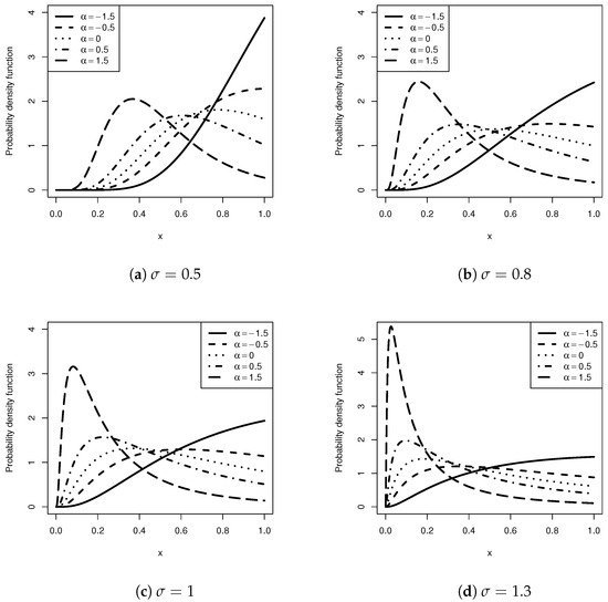
Figure 1. Graph of the UTPN densities for various values of $\alpha$ and $\sigma$.

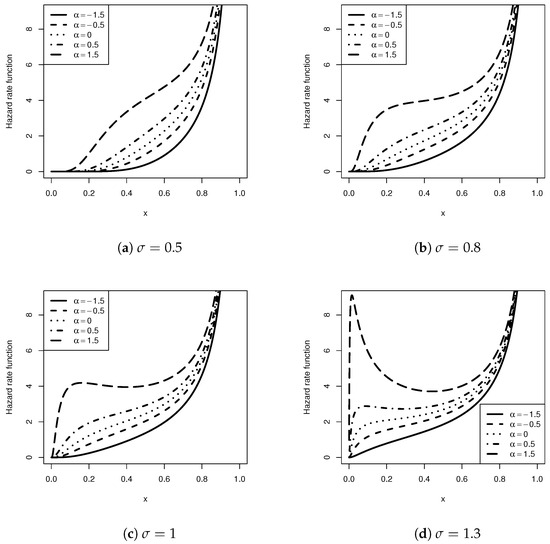
Figure 2. Graphs of the HR function for the UTPN distribution with varying values of $\alpha$ and $\sigma$.

2.3. Quantile Function

The quantile function of the UTPN distribution is derived by inverting Equation (4) as follows:

$$Q_p={\left(\exp \left\{{\Phi }^{-1}\left(\frac{p}{c_{\alpha }}\right)-\alpha \right\}\right)}^{\sigma },0<p<1.$$

(9)

Note that $Q_{0.5}$, $Q_{0.25}$, and $Q_{0.75}$ stand for median, first quartile, and third quartile of the UTPN distribution, correspondingly.

2.4. Mode

The mode of $f_X(x;\alpha ,\sigma )$ is the root of the equation

$$\frac{d}{dx}\log \left(f_X(x;\alpha ,\sigma )\right)=-\frac{1}{x}-\frac{1}{x\sigma }\left(\frac{\log \left(x\right)}{\sigma }+\alpha \right)=0.$$

(10)

Therefore, if $x=x_0$,

$$x_0=\exp \left\{-{\sigma }^2\left(1+\frac{\alpha }{\sigma }\right)\right\},$$

(11)

this means that $x_0$ is the sole point where $f_X(x;\alpha ,\sigma )$ reaches its maximum.

2.5. Hazard Rate Function

Lemma 1.

Given that $f\left(x\right)$, for $x>0$, is a twice-differentiable density function of a positive real-valued continuous random variable with an HR function $h\left(x\right)$, let $\lambda \left(x\right)=-(d/dx)\log \left(f\right(x\left)\right)$. Consequently, (i) if $\lambda \left(x\right)$ decreases (increases) as x increases, then $h\left(x\right)$ increases (decreases) as x increases, and (ii) if $\lambda \left(x\right)$ follows a bathtub (inverted bathtub) pattern, then $h\left(x\right)$ will also follow a bathtub (inverted bathtub) pattern.

The proof of this result is provided by Glaser [21]. Based on this finding, the shape of the HR function of the UTPN distribution can be inferred as follows.

Proposition 2.

The HR function of the UTPN distribution exhibits an inverted bathtub shape.

Proof. 

Given that

$$\lambda \left(x\right)=\frac{\sigma (\alpha +\sigma )+\log \left(x\right)}{x{\sigma }^2},$$

(12)

it follows that

$$\frac{d}{dx}\lambda \left(x\right)=\frac{-\sigma (\alpha +\sigma )-\log \left(x\right)+1}{x^2{\sigma }^2}.$$

(13)

Consequently, by ${\lambda }^{\prime }\left(x\right)=0$, the global maximum of $\lambda \left(x\right)$ is $x_{\ast }=\exp \{1-\sigma (\alpha +\sigma )\}$, because

$${\left.\frac{d^2}{d{x}^2}\lambda \left(x\right)\right|}_{x=x_{\ast }}=\frac{-1}{{\sigma }^2\exp \{3-3\sigma (\alpha +\sigma )\}}<0.$$

(14)

This demonstrates that $\lambda \left(x\right)$ exhibits an inverted bathtub shape. Therefore, according to Glaser’s Lemma, $h\left(x\right)$ also exhibits an inverted bathtub shape. Additionally, with $(d/dx)\lambda \left(x\right)>0$ for $x\in (0,1)$, $\sigma >0$, and $\alpha <-\sigma$, it follows that $\lambda \left(x\right)$ is an increasing function. □

2.6. Moments and Moment Generating Function

Here, we derive the expressions for the moments and moment-generating function of the distribution, which are crucial for any statistical analysis, particularly in applied research. The distribution’s moments, including its mean, variance, skewness, and kurtosis, provide insight into its most significant characteristics.

Proposition 3.

If the random variable X follows a UTPN distribution, its r-th moment about zero can be calculated as

$$\mathbb{E}\left(X^r\right)=\frac{\Phi (\alpha -r\sigma )}{\Phi \left(\alpha \right)}\exp \left\{\sigma \left(\frac{r^2\sigma }{2}-\alpha \right)\right\}.$$

(15)

Proof. 

Using the stochastic representation $X=\exp \{-Z\}$, where $Z\sim TPN(\sigma ,\alpha )$, one can write

$$\mathbb{E}\left(X^r\right)=\mathbb{E}\left(e^{-rZ}\right)={\int }_0^{\infty }\frac{c_{\alpha }}{\sigma }{e}^{-rz}\varphi \left(\frac{z}{\sigma }-\alpha \right)dz$$

and defining $u=z/\sigma -\alpha$ implies

$$\mathbb{E}\left(X^r\right)={\int }_{-\alpha }^{\infty }{c}_{\alpha }{e}^{-r\sigma (u+\alpha )}\varphi \left(u\right)du=\frac{\Phi (\alpha -r\sigma )}{\Phi \left(\alpha \right)}\exp \left\{\sigma \left(\frac{r^2\sigma }{2}-\alpha \right)\right\}.$$

This is accomplished using some simplifications and minor algebraic manipulation. □

Corollary 1.

(i) Let $X\sim UTPN(\alpha ,\sigma )$; then, the mean, variance, skewness (${\gamma }_X$), and kurtosis (${\kappa }_X$) coefficients are, respectively, given as

$$\mathbb{E}\left(X\right)={\rho }_1{e}^{\sigma (\frac{\sigma }{2}-\alpha )},Var\left(X\right)=e^{\sigma (\sigma -2\alpha )}({\rho }_2{e}^{{\sigma }^2}-{\rho }_1^2),$$

$${\gamma }_X=\frac{{\rho }_3{e}^{3{\sigma }^2}-3{\rho }_1{\rho }_2{e}^{{\sigma }^2}+2{\rho }_1^3}{{({\rho }_2{e}^{{\sigma }^2}-{\rho }_1^2)}^{3/2}}and{\kappa }_X=\frac{{\rho }_4{e}^{6{\sigma }^2}-4{\rho }_1{\rho }_3{e}^{3{\sigma }^2}+6{\rho }_1^2{\rho }_2{e}^{{\sigma }^2}-3{\rho }_1^4}{{({\rho }_2{e}^{{\sigma }^2}-{\rho }_1^2)}^2},$$

(ii) As a result of the central limit theorem, let $X_1,X_2,\dots$ be independent random variables, and utilizing the identical distribution of $X\sim UTPN(\alpha ,\sigma )$, then, if $S_n=X_1+X_2+\dots +X_n$, one has

$$\frac{S_n-n\mu }{\omega \sqrt{n}}\stackrel{\mathcal{D}}{\to }N(0,1)(n\uparrow \infty ),$$

where

$$\mu ={\rho }_1\exp \left\{\sigma \left(\sigma /2-\alpha \right)\right\},\omega =\sqrt{\exp \left\{\sigma (\sigma -2\alpha )\right\}({\rho }_2\exp \left\{{\sigma }^2\right\}-{\rho }_1^2)},$$

$${\rho }_r:={\rho }_r(\sigma ,\alpha )=\frac{\Phi (\alpha -r\sigma )}{\Phi \left(\alpha \right)} \mathit{and} =r=1,2,3,4.$$

In Figure 3, the UTPN distribution’s mean, variance, skewness, and kurtosis are displayed as functions of $\alpha$ and $\sigma$. Observations indicate that as $\alpha$ varies, the mean decreases independently of the values of $\sigma$. In terms of variance, the curves exhibit concavity and unimodality for all $\alpha$ values, with values decreasing as $\sigma$ decreases. On the other hand, negative skewness is observed for $\alpha <0$, while positive skewness is observed for $\alpha >0$. In addition, smaller $\sigma$ values are associated with reduced skewness, while larger $\sigma$ values are associated with increased skewness. Finally, kurtosis decreases as $\sigma$ decreases, which occurs for $\alpha >2$ (approximately).

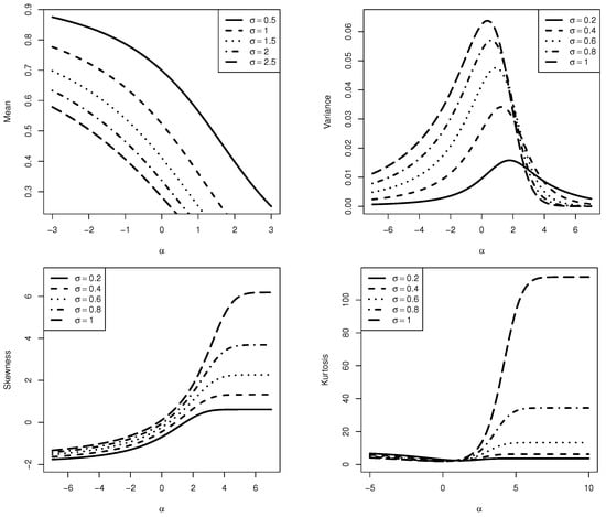
Figure 3. Graph of the UTPN distribution’s mean, variance, skewness, and kurtosis for various values of $\alpha$ and $\sigma$.

Proposition 4.

If the random variable X is UTPN distributed, then its moment-generating function is given by

$$M_X\left(t\right)=\mathbb{E}\left(e^{tX}\right)=\sum _{k=0}^{\infty }\frac{t^k}{k!}{\rho }_k(\sigma ,\alpha )\exp \left\{k\sigma \left(\frac{k\sigma }{2}-\alpha \right)\right\}.$$

(16)

Proof. 

The moment-generating function’s definition implies

$$M_X\left(t\right)=c_{\alpha }{\int }_0^1\frac{e^{tx}}{x\sigma }\varphi \left(\frac{\log \left(x\right)}{\sigma }+\alpha \right)dx,$$

using the exponential series $\exp \left\{a\right\}={\sum }_{k=0}^{\infty }{a}^k/k!$ and taking the change of variables $u=\log \left(x\right)/\sigma +\alpha$

$$\begin{array}{ccc}\hfill M_X\left(t\right)& =& c_{\alpha }{\int }_{-\infty }^{\alpha }\sum _{k=0}^{\infty }\frac{t^k{e}^{k(u-\alpha )\sigma }}{k!}\varphi \left(u\right)du\hfill \\ & =& c_{\alpha }\sum _{k=0}^{\infty }\frac{t^k{e}^{-k\alpha \sigma }}{k!}{\int }_{-\infty }^{\alpha }{e}^{k\sigma u}\varphi \left(u\right)du\hfill \\ & =& \sum _{k=0}^{\infty }\frac{t^k{e}^{k\sigma (\frac{k\sigma }{2}-\alpha )}}{k!}\frac{\Phi (\alpha -k\sigma )}{\Phi \left(\alpha \right)}\hfill \\ & =& \sum _{k=0}^{\infty }\frac{t^k}{k!}{\rho }_k(\sigma ,\alpha )\exp \left\{k\sigma \left(\frac{k\sigma }{2}-\alpha \right)\right\}.\hfill \end{array}$$

 □

2.7. Curves of Bonferroni and Lorenz

Bonferroni and Lorenz curves [22] are commonly used in economics to study income and poverty, although they are also helpful in other domains, including reliability, insurance, demography, and medicine. The definition of the Bonferroni curve is

$$B\left(p\right)=\frac{1}{p\mu }{\int }_0^{q}x{f}_X\left(x\right)dx,0\le p<1,$$

(17)

where $\mu =\mathbb{E}\left(X\right)$ and $q=F_X^{-1}(p;\alpha ,\sigma )$. The Lorenz curve is obtained by the expression $L\left(p\right)=pB\left(p\right)$. Specifically, the Bonferroni curve for the UTPN distribution can be calculated as

$$B\left(p\right)=\frac{c_{\alpha }}{p\mu }\Phi \left(\frac{\log \left(q\right)}{\sigma }+\alpha -\sigma \right)\exp \left\{\sigma \left(\frac{\sigma }{2}-\alpha \right)\right\}.$$

Figure 4 illustrates the Bonferroni curve for the UTPN distribution with $\sigma =1$, showing different values for $\alpha$. It is clear that the Bonferroni value increases as $\alpha$ decreases. Additionally, the graph indicates that as the probability p increases, the Bonferroni value also increases.

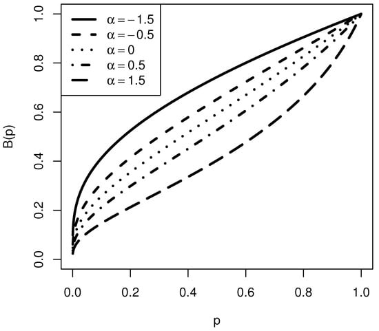
Figure 4. Bonferroni curve for the UTPN distribution for $\alpha =-1.5,-0.5,0,0.5,1.5$ and $\sigma =1$.

2.8. Entropy

A measure of the uncertainty’s variation is the entropy of a random variable X with a certain PDF. Greater data uncertainty is indicated by a high entropy value. The Rényi entropy [23], $R_{\lambda }\left(X\right)$, for X is defined as

$$R_{\lambda }\left(X\right)=\frac{1}{1-\lambda }\log \left\{{\int }_{\mathbb{R}}{f}_X^{\lambda }\left(x\right)dx\right\},$$

(18)

where $\lambda >0$ and $\lambda \ne 1$. Suppose X has the UTPN distribution, then by substituting (3) in (18), we obtain

$$\begin{array}{ccc}\hfill {\int }_{\mathbb{R}}{f}_X^{\lambda }\left(x\right)dx& =& {\int }_0^1\frac{c_{\alpha }^{\lambda }}{{\sigma }^{\lambda }{x}^{\lambda }}{\varphi }^{\lambda }\left(\frac{\log \left(x\right)}{\sigma }+\alpha \right)dx\hfill \\ & =& \frac{c_{\alpha }^{\lambda }}{{\sigma }^{\lambda -1}}{\int }_{-\infty }^{\alpha }{e}^{\sigma (u-\alpha )(1-\lambda )}{\varphi }^{\lambda }\left(u\right)du\hfill \\ & =& c_{\alpha }^{\lambda }{\sigma }^{1-\lambda }{\lambda }^{-1/2}{\left(2\pi \right)}^{(1-\lambda )/2}\Phi \left(\frac{\alpha \lambda -(1-\lambda )\sigma }{\sqrt{\lambda }}\right)\exp \left\{\frac{{(1-\lambda )}^2{\sigma }^2}{2\lambda }-\alpha (1-\lambda )\sigma \right\}.\hfill \end{array}$$

So one obtains the Rényi entropy as follows:

$$R_{\lambda }\left(X\right)=-\alpha \sigma +\log \left(\sigma \sqrt{2\pi }\right)+\frac{(1-\lambda ){\sigma }^2}{2\lambda }-\frac{\log \left(\lambda \right)}{2(1-\lambda )}+\frac{1}{1-\lambda }\log \Phi \left(\frac{\alpha \lambda -(1-\lambda )\sigma }{\sqrt{\lambda }}\right)-\frac{\lambda }{1-\lambda }\log \Phi \left(\alpha \right).$$

Shannon entropy [24] defined by $S_{\lambda }\left(X\right)=\mathbb{E}\{-\log \left(f_X\left(x\right)\right)\}$ is the particular case of Equation (18) when $\lambda \to 1$. Then calculating the ${lim}_{\lambda \to 1}{R}_{\lambda }\left(X\right)$ and using L’Hospital’s rule, after some algebraic work, one obtains the result that

$$S_{\lambda }\left(X\right)=\log \left(\sigma \sqrt{2\pi }\Phi \left(\alpha \right)\exp \left\{\alpha \sigma -\frac{1}{2}\right\}\right)-\frac{c_{\alpha }}{2}(\alpha +2\sigma )\varphi \left(\alpha \right).$$

3. Estimation and Inference

In this section, we use the maximum likelihood and moments approaches to estimate the distribution parameters with the related inference.

3.1. Moments Estimator

Assume that the collection of realizations $x_1,\dots ,x_n$ comes from a size-n random sample selected from the UTPN distribution with parameters $\alpha \in \mathbb{R}$ and $\sigma >0$. For the moments estimation, let $m_1=(1/n){\sum }_{i=1}^n{x}_i$, $m_2=(1/n){\sum }_{i=1}^n{x}_i^2$, ${\rho }_1=\Phi (\alpha -\sigma )/\Phi \left(\alpha \right)$ and ${\rho }_2=\Phi (\alpha -2\sigma )/\Phi \left(\alpha \right)$. By equating the theoretical moments obtained by Corollary 1 with the sample moments given above, one obtains the following equations:

$$\begin{array}{ccc}\hfill \sigma \left(\frac{\sigma }{2}-\alpha \right)& =& \log \left(\frac{m_1}{{\rho }_1}\right)\hfill \\ \hfill 2\sigma (\sigma -\alpha )& =& \log \left(\frac{m_2}{{\rho }_2}\right).\hfill \end{array}$$

The moment estimators for $\alpha$ and $\sigma$ are calculated by simultaneously solving these equations with an appropriate numerical method.

3.2. Maximum Likelihood Estimator

Here, we derive the maximum likelihood estimators (MLEs) and the observed Fisher information matrix for complete samples of the UTPN distribution. Let $\mathit{x}=(x_1,\dots ,x_n)$ denote the observed values obtained from a size-n random sample selected from the UTPN distribution with parameters $\alpha \in \mathbb{R}$ and $\sigma >0$. We assume that both $\alpha$ and $\sigma$ are unknown and aim to estimate them based on $\mathit{x}$. In this context, we adopt the maximum likelihood approach. The likelihood function for $\alpha$ and $\sigma$, given $\mathit{x}$, is expressed as

$$L(\alpha ,\sigma )=\frac{c_{\alpha }^n}{{\sigma }^n}\prod _{i=1}^n{x}_i^{-1}\varphi \left(\frac{\log \left(x_i\right)}{\sigma }+\alpha \right).$$

Hence, the following is an expression for the log-likelihood function:

$$\mathit{\ell }(\alpha ,\sigma )=n\log \left(c_{\alpha }\right)-n\log \left(\sigma \right)+\sum _{i=1}^n\log \left\{\varphi \left(\frac{\log \left(x_i\right)}{\sigma }+\alpha \right)\right\}-\sum _{i=1}^n\log \left(x_i\right).$$

The function $l(\alpha ,\sigma )$ is well defined for all values of the model parameters. It is continuous and concave with respect to the parameters, ensuring the existence of a unique global maximum. Additionally, the parameter space is bounded, which contributes to the uniqueness of the MLE. These properties guarantee that the MLE is unique and exists for the proposed distribution (Casella and Berger [25]). Therefore, in accordance with the conditions described above, the MLEs of $\alpha$ and $\sigma$ are defined by

$$(\widehat{\alpha },\widehat{\sigma })={\mathrm{a}\mathrm{r}\mathrm{g}\mathrm{m}\mathrm{a}\mathrm{x}}_{(\alpha ,\sigma )\in \mathbb{R}\times {\mathbb{R}}^{+}}\mathit{\ell }(\alpha ,\sigma ).$$

That is, $\widehat{\alpha }$ and $\widehat{\sigma }$ fulfill the score equations linked to ${\left.\partial \mathit{\ell }(\alpha ,\sigma )/\partial \alpha \right|}_{\alpha =\widehat{\alpha },\sigma =\widehat{\sigma }}=0$,

$${\left.-n(\alpha +c_{\alpha }\varphi \left(\alpha \right))-\frac{1}{\sigma }\sum _{i=1}^n\log \left(x_i\right)\right|}_{\alpha =\widehat{\alpha },\sigma =\widehat{\sigma }}=0,$$

(19)

and ${\left.\partial \mathit{\ell }(\alpha ,\sigma )/\partial \sigma \right|}_{\alpha =\widehat{\alpha },\sigma =\widehat{\sigma }}=0$ implies

$${\left.-\frac{n}{\sigma }+\frac{\alpha }{{\sigma }^2}\sum _{i=1}^n\log \left(x_i\right)+\frac{1}{{\sigma }^3}\sum _{i=1}^n{\log }^2\left(x_i\right)\right|}_{\alpha =\widehat{\alpha },\sigma =\widehat{\sigma }}=0.$$

(20)

We focus on the existence and uniqueness of each MLE of the distribution parameters in the following theorems, assuming that the other parameter is known; for additional details on this method, see Popović et al. [26] and Alomair et al. [27].

Proposition 5.

Given (19), there exists a unique solution to the equation $\partial \mathit{\ell }(\alpha ,\sigma )/\partial \alpha =0$ for $\alpha \in \mathbb{R}$.

Proof. 

We have

$$\frac{\partial \mathit{\ell }(\alpha ,\sigma )}{\partial \alpha }=-n\left(\frac{\varphi \left(\alpha \right)}{\Phi \left(\alpha \right)}+\alpha \right)-\frac{1}{\sigma }\sum _{i=1}^n\log \left(x_i\right).$$

We know that $\varphi \left(\alpha \right)\to 0$ as $\alpha \to \pm \infty$, $\Phi \left(\alpha \right)\to 1$ as $\alpha \to \infty$, and $\Phi \left(\alpha \right)\to 0$ as $\alpha \to -\infty$. Thus, $-n\left(\varphi \right(\alpha )/\Phi (\alpha )+\alpha )\to 0$ as $\alpha \to -\infty$ and $-n\left(\varphi \right(\alpha )/\Phi (\alpha )+\alpha )\to -\infty$ as $\alpha \to \infty$. On the other hand, it follows that ${lim}_{\alpha \to -\infty }\partial \mathit{\ell }(\alpha ,\sigma )/\partial \alpha =-(1/\sigma ){\sum }_{i=1}^n\log \left(x_i\right)>0$ (because $\sigma >0$ and $\log \left(x_i\right)<0,\forall i=1,\dots ,n$) and ${lim}_{\alpha \to \infty }\partial \mathit{\ell }(\alpha ,\sigma )/\partial \alpha =-\infty$. Therefore, there exists at least one root, say $\widehat{\alpha }\in (-\infty ,\infty )$, such that ${\left.\partial \mathit{\ell }(\alpha ,\sigma )/\partial \alpha \right|}_{\alpha =\widehat{\alpha },\sigma }=0$. To prove uniqueness, we need to verify that ${\partial }^2\mathit{\ell }(\alpha ,\sigma )/\partial {\alpha }^2<0$. Indeed, $-n<{\partial }^2\mathit{\ell }(\alpha ,\sigma )/\partial {\alpha }^2<0$ for all $n\ge 1$, because

$$\underset{\alpha \to -\infty }{lim}\frac{{\partial }^2\mathit{\ell }(\alpha ,\sigma )}{\partial {\alpha }^2}=\underset{\alpha \to -\infty }{lim}-n\left(1-{\left(\frac{\varphi \left(\alpha \right)}{\Phi \left(\alpha \right)}\right)}^2-\alpha \frac{\varphi \left(\alpha \right)}{\Phi \left(\alpha \right)}\right)=0$$

and

$$\underset{\alpha \to \infty }{lim}\frac{{\partial }^2\mathit{\ell }(\alpha ,\sigma )}{\partial {\alpha }^2}=\underset{\alpha \to \infty }{lim}-n\left(1-{\left(\frac{\varphi \left(\alpha \right)}{\Phi \left(\alpha \right)}\right)}^2-\alpha \frac{\varphi \left(\alpha \right)}{\Phi \left(\alpha \right)}\right)=-n<0.$$

Therefore, there exists a solution to $\partial \mathit{\ell }(\alpha ,\sigma )/\partial \alpha =0$ and the root $\widehat{\alpha }$ is unique. □

Proposition 6.

Given (20), there exists a solution for equation $\partial \mathit{\ell }(\alpha ,\sigma )/\partial \sigma =0$ for $\sigma >0$, and the solution is unique when $n{\sigma }^2<S(\alpha ,\sigma )$, where

$$S(\alpha ,\sigma )=2\alpha \sigma \sum _{i=1}^n\log \left(x_i\right)+3\sum _{i=1}^n{\log }^2\left(x_i\right).$$

Proof. 

Solving $\partial \mathit{\ell }(\alpha ,\sigma )/\partial \sigma =0$ is equivalent to solving $h(\alpha ,\sigma )=0$, where

$$h(\alpha ,\sigma )=-n{\sigma }^2+\alpha \sigma \sum _{i=1}^n\log \left(x_i\right)+\sum _{i=1}^n{\log }^2\left(x_i\right).$$

For known $\alpha$, and knowing that ${\log }^2\left(x_i\right)>0$ for all $i=1,\dots ,n$, we have the limit values of $h(\alpha ,\sigma )$ as follows

$$\underset{\sigma \to 0}{lim}h(\alpha ,\sigma )=\sum _{i=1}^n{\log }^2\left(x_i\right)>0\mathrm{and}\underset{\sigma \to \infty }{lim}h(\alpha ,\sigma )=-\infty .$$

Thus we can ensure that there is at least one root, say $\widehat{\sigma }\in (0,\infty )$, such that $h(\alpha ,\widehat{\sigma })=0$. To prove uniqueness, we have to show that ${\partial }^2\mathit{\ell }(\alpha ,\sigma )/\partial {\sigma }^2<0$; that is,

$$\frac{n}{{\sigma }^2}-\frac{2\alpha }{{\sigma }^3}\sum _{i=1}^n\log \left(x_i\right)-\frac{3}{{\sigma }^4}\sum _{i=1}^n{\log }^2\left(x_i\right)<0,$$

which implies

$$\begin{array}{ccc}\hfill \frac{n}{{\sigma }^2}& <& \frac{2\alpha }{{\sigma }^3}\sum _{i=1}^n\log \left(x_i\right)+\frac{3}{{\sigma }^4}\sum _{i=1}^n{\log }^2\left(x_i\right),\hfill \\ \hfill n{\sigma }^2& <& 2\alpha \sigma \sum _{i=1}^n\log \left(x_i\right)+3\sum _{i=1}^n{\log }^2\left(x_i\right).\hfill \end{array}$$

Hence, we find that $n{\sigma }^2<S(\alpha ,\sigma )$. Therefore, there exists a solution to $\partial \mathit{\ell }(\alpha ,\sigma )/\partial \sigma =0$, and the root $\widehat{\sigma }$ is unique when $n{\sigma }^2<S(\alpha ,\sigma )$. □

From (19), it follows immediately that the MLE of $\sigma$ can be obtained as

$$\widehat{\sigma }=-\frac{\overline{\log \left(x\right)}}{c_{\widehat{\alpha }}\varphi \left(\widehat{\alpha }\right)+\widehat{\alpha }}.$$

(21)

Using (20) and (21), the MLE of $\alpha$ satisfies the following equation

$$\frac{1}{c_{\widehat{\alpha }}\varphi \left(\widehat{\alpha }\right)+\widehat{\alpha }}\left(\frac{1}{c_{\widehat{\alpha }}\varphi \left(\widehat{\alpha }\right)+\widehat{\alpha }}+\widehat{\alpha }\right)=\frac{\overline{{\log }^2\left(x\right)}}{{\left(\overline{\log \left(x\right)}\right)}^2}.$$

where $\overline{\log \left(x\right)}=(1/n){\sum }_{i=1}^n\log \left(x_i\right)$ and $\overline{{\log }^2\left(x\right)}=(1/n){\sum }_{i=1}^n{\log }^2\left(x_i\right)$.

The numerical values of $\widehat{\alpha }$ and $\widehat{\sigma }$ can be determined via any statistical software. Theoretical results guarantee the convergence of the MLEs in any sense, as well as the desired asymptotic normality.

The proof of the MLEs’ asymptotic normality is provided in the following proposition.

Proposition 7.

Let $\theta =(\alpha ,\sigma )$ and suppose that the regularity conditions (Casella and Berger [25]) hold for $f_X(x;\theta )$ such that ${\partial }^3\mathit{\ell }\left(\theta \right)/\partial {\theta }^3$ exists and its absolute value is bounded by a function $K\left(x\right)$ such that $\mathbb{E}\left(K\right(X\left)\right)\le k$.

Let ${\left\{\widehat{\theta }\right\}}_n$ be a consistent sequence of roots of $S\left(\theta \right)=\partial \mathit{\ell }\left(\theta \right)/\partial \theta$, i.e., $\widehat{\theta }\stackrel{\mathcal{P}}{⟶}{\theta }_0$, where ${\theta }_0$ is the true value of the parameter. Then,

$$\sqrt{n}(\widehat{\theta }-{\theta }_0)\stackrel{\mathcal{D}}{⟶}N(0,{\mathcal{I}}^{-1}\left({\theta }_0\right)),$$

where

$$\mathcal{I}\left({\theta }_0\right)={\left.\mathbb{E}\left(-\frac{{\partial }^2\mathit{\ell }\left(\theta \right)}{\partial {\theta }^2}\right)\right|}_{\theta ={\theta }_0}.$$

Proof. 

We perform a second-order Taylor expansion of the score function $S\left(\theta \right)$ around ${\theta }_0$ and evaluate it at $\widehat{\theta }$:

$$0=S\left(\widehat{\theta }\right)=S\left({\theta }_0\right)+(\widehat{\theta }-{\theta }_0)\frac{\partial S\left({\theta }_0\right)}{\partial \theta }+\frac{1}{2}{(\widehat{\theta }-{\theta }_0)}^2\frac{{\partial }^{2}S\left({\theta }^{\ast }(\widehat{\theta },{\theta }_0)\right)}{\partial {\theta }^2},$$

where $|{\theta }^{\ast }(\widehat{\theta },{\theta }_0)-{\theta }_0|\le |\widehat{\theta }-{\theta }_0|$. Dividing by $\sqrt{n}$ we get

$$0=\frac{1}{\sqrt{n}}S\left({\theta }_0\right)+\sqrt{n}(\widehat{\theta }-{\theta }_0)\left[\frac{1}{n}\frac{\partial S\left({\theta }_0\right)}{\partial \theta }+\frac{1}{2n}(\widehat{\theta }-{\theta }_0)\frac{{\partial }^{2}S\left({\theta }^{\ast }(\widehat{\theta },{\theta }_0)\right)}{\partial {\theta }^2}\right].$$

(22)

By the central limit theorem,

$$\frac{1}{\sqrt{n}}S\left({\theta }_0\right)={\left.\frac{1}{\sqrt{n}}\sum _{i=1}^n\frac{\partial \log f_X(X_i;\theta )}{\partial \theta }\right|}_{\theta ={\theta }_0}\stackrel{\mathcal{D}}{⟶}N(0,\mathcal{I}\left({\theta }_0\right)),$$

since $\partial \log f_X(X_i;\theta )/\partial \theta$ are i.i.d. random variables with mean zero and variance and $\mathcal{I}\left({\theta }_0\right)<\infty$.

Also, by the weak law of large numbers,

$$-\frac{1}{n}\frac{\partial S\left({\theta }_0\right)}{\partial \theta }={\left.-\frac{1}{n}\sum _{i=1}^n\frac{{\partial }^2\log f_X(X_i;\theta )}{\partial {\theta }^2}\right|}_{\theta ={\theta }_0}\stackrel{\mathcal{P}}{⟶}\mathcal{I}\left({\theta }_0\right).$$

Using the law of large numbers, we have

$$\frac{1}{n}\left|\frac{{\partial }^{2}S\left({\theta }^{\ast }(\widehat{\theta },{\theta }_0)\right)}{\partial {\theta }^2}\right|\le \frac{1}{n}\sum _{i=1}^n{\left|\frac{{\partial }^3\log f_X(X_i;\theta )}{\partial {\theta }^3}\right|}_{\theta ={\theta }^{\ast }}\le \frac{1}{n}\sum _{i=1}^{n}K\left(X_i\right)\stackrel{\mathcal{P}}{⟶}\mathbb{E}\left(K\left(X\right)\right)<k,$$

i.e., $|{\partial }^{2}S\left({\theta }^{\ast }(\widehat{\theta },{\theta }_0)\right)/\partial {\theta }^2|/n$ is bounded in probability by the constant k: for any $\epsilon >0$, the probability that it is less than $k+\epsilon$ approaches 1. Finally, since $\widehat{\theta }\stackrel{\mathcal{P}}{⟶}{\theta }_0$, we have

$$\frac{1}{2n}(\widehat{\theta }-{\theta }_0)\frac{{\partial }^{2}S\left({\theta }^{\ast }(\widehat{\theta },{\theta }_0)\right)}{\partial {\theta }^2}\stackrel{\mathcal{P}}{⟶}0.$$

Employing Equation (22) and combining the previous results, we obtain

$$\sqrt{n}(\widehat{\theta }-{\theta }_0)=\frac{\stackrel{\stackrel{\mathcal{D}}{⟶}N(0,\mathcal{I}\left({\theta }_0\right))}{\overbrace{\frac{1}{\sqrt{n}}S\left({\theta }_0\right)}}}{-\underset{\stackrel{\mathcal{P}}{⟶}\mathcal{I}\left({\theta }_0\right)}{\underbrace{\frac{1}{n}\frac{\partial S\left({\theta }_0\right)}{\partial \theta }}}-\underset{\stackrel{\mathcal{P}}{⟶}0}{\underbrace{\frac{1}{2n}(\widehat{\theta }-{\theta }_0)\frac{{\partial }^{2}S\left({\theta }^{\ast }(\widehat{\theta },{\theta }_0)\right)}{\partial {\theta }^2}}}},$$

and by Slutsky’s theorem, we conclude that

$$\sqrt{n}(\widehat{\theta }-{\theta }_0)\stackrel{\mathcal{D}}{⟶}N(0,{\mathcal{I}}^{-1}\left({\theta }_0\right)).$$

 □

In the Appendix A of this article, the entries of the information matrix are calculated, resulting in

$$\mathcal{I}\left({\theta }_0\right)=n\left(\begin{array}{cc}1-c_{\alpha }^2{\varphi }^2\left(\alpha \right)-\alpha c_{\alpha }\varphi \left(\alpha \right)& \frac{1}{\sigma }(\alpha +c_{\alpha }\varphi \left(\alpha \right))\\ \frac{1}{\sigma }(\alpha +c_{\alpha }\varphi \left(\alpha \right))& \frac{1}{{\sigma }^2}(2+{\alpha }^2+\alpha c_{\alpha }\varphi \left(\alpha \right))\end{array}\right).$$

On the other hand, using the previous results, we have that $\widehat{\theta }\sim N_2(\theta ,{\Sigma }^{-1}\left(\widehat{\theta }\right))$, where

$${\Sigma }^{-1}\left(\widehat{\theta }\right)=\frac{1}{\left|\mathcal{I}\right(\widehat{\theta }\left)\right|}\left(\begin{array}{cc}\frac{1}{{\widehat{\sigma }}^2}(2+{\widehat{\alpha }}^2+\widehat{\alpha }{c}_{\widehat{\alpha }}\varphi \left(\widehat{\alpha }\right))& -\frac{1}{\widehat{\sigma }}(\widehat{\alpha }+c_{\widehat{\alpha }}\varphi \left(\widehat{\alpha }\right))\\ -\frac{1}{\widehat{\sigma }}(\widehat{\alpha }+c_{\widehat{\alpha }}\varphi \left(\widehat{\alpha }\right))& 1-c_{\widehat{\alpha }}^2{\varphi }^2\left(\widehat{\alpha }\right)-\widehat{\alpha }{c}_{\widehat{\alpha }}\varphi \left(\widehat{\alpha }\right)\end{array}\right),$$

(23)

is the inverse of the observed information matrix and $|\mathcal{I}\left(\widehat{\theta }\right)|=n^2\mathcal{J}\left(\widehat{\theta }\right)/{\widehat{\sigma }}^2$ is the determinant of the matrix $\mathcal{I}\left(\widehat{\theta }\right)$, where $\mathcal{J}\left(\widehat{\theta }\right)=2-\widehat{\alpha }{c}_{\widehat{\alpha }}^3{\varphi }^3\left(\widehat{\alpha }\right)-\widehat{\alpha }{c}_{\widehat{\alpha }}\varphi \left(\widehat{\alpha }\right)(3+{\widehat{\alpha }}^2)-c_{\widehat{\alpha }}^2{\varphi }^2\left(\widehat{\alpha }\right)(3+2{\widehat{\alpha }}^2)$.

By using (23), we find that approximately $100(1-\beta )\%$ asymptotic confidence intervals for $\alpha$ and $\sigma$ are

$$\widehat{\alpha }\pm \frac{z_{\beta /2}}{n}\sqrt{\frac{2+{\widehat{\alpha }}^2+\widehat{\alpha }{c}_{\widehat{\alpha }}\varphi \left(\widehat{\alpha }\right)}{\mathcal{J}\left(\widehat{\theta }\right)}}\mathrm{a}\mathrm{n}\mathrm{d}\widehat{\sigma }\left(1\pm \frac{z_{\beta /2}}{n}\right)\sqrt{\frac{1-c_{\widehat{\alpha }}^2{\varphi }^2\left(\widehat{\alpha }\right)-\widehat{\alpha }{c}_{\widehat{\alpha }}\varphi \left(\widehat{\alpha }\right)}{\mathcal{J}\left(\widehat{\theta }\right)}},$$

where $z_{\beta /2}$ is the upper $\beta$-th percentile of the SN distribution.

We will use the Kolmogorov–Smirnov (K-S) test to assess the goodness-of-fit for the proposed models. The K-S test statistic D is defined as the maximum absolute difference between the empirical cumulative distribution function (ECDF) of the sample and the CDF of the reference distribution: $D={sup}_x|F_n\left(x\right)-F\left(x\right)|$, where $F_n\left(x\right)$ is the ECDF of the sample and $F\left(x\right)$ is the theoretical CDF. Additionally, to evaluate the fit of various models, we will employ the maximum likelihood technique and well-known fitting criteria, specifically the Hannan–Quinn information criterion (HQIC), the Bayesian information criterion (BIC), the consistent Akaike’s information criterion (CAIC), and the Akaike information criterion (AIC). For the UTPN model, these criteria are defined as follows:

$$\begin{array}{cccc}\hfill \mathrm{AIC}& =-2\mathit{\ell }\left(\widehat{\theta }\right)+2m,\hfill & \hfill \mathrm{CAIC}& =-2\mathit{\ell }\left(\widehat{\theta }\right)+\frac{2mn}{n-m-1},\hfill \\ \hfill \mathrm{BIC}& =-2\mathit{\ell }\left(\widehat{\theta }\right)+m\log \left(n\right),\hfill & \hfill \mathrm{HQIC}& =-2\mathit{\ell }\left(\widehat{\theta }\right)+2m\log \left(\log \left(n\right)\right),\hfill \end{array}$$

where m is the number of parameters. The R programming language (see [28]) will be utilized for the simulation and practical aspects, as discussed in the next section.

4. Simulation Study

This section examines the performance of the MLEs and the asymptotic confidence intervals for the parameters indexing the UTPN distribution through Monte Carlo simulations. The sample size is set at $n=25$, 35, 50, 100, 200, and 500, while the parameters are fixed at $\alpha =$ −$0.3$, 0.3, and 4.5, with $\sigma =0.4$ and 2.3. For each combination, $M=10,000$ pseudo-random samples are generated from the UTPN distribution using the inverse CDF method, meaning

$$x={\left(\exp \left\{{\Phi }^{-1}\left(\frac{u}{c_{\alpha }}\right)-\alpha \right\}\right)}^{\sigma },$$

(24)

where u is a uniform $(0,1)$ observation.

To assess the performance of the MLEs and their asymptotic confidence intervals, the bias (Bias), standard error (SE), root mean squared error (RMSE), and coverage probability (CP) of the 95% confidence intervals are calculated. Insights can be gleaned from Table 1.

Table 1. Empirical mean, bias, SE, RMSE, and 95% CP for the ML estimates of $\alpha$ and $\sigma$ in the UTPN distribution across different combinations of $\alpha$ and $\sigma$ parameters.

True Value		n	Estimate	Mean	Bias	SE	RMSE	CP
$\alpha =$ −$0.3$	$\sigma =0.4$	25	$\widehat{\alpha }$	−0.2569	0.0431	1.7876	1.4398	0.8744
			$\widehat{\sigma }$	0.4123	0.0123	0.3403	0.2745	0.8112
		35	$\widehat{\alpha }$	−0.3351	−0.0351	1.5696	1.1978	0.8958
			$\widehat{\sigma }$	0.4227	0.0227	0.3062	0.2296	0.8391
		50	$\widehat{\alpha }$	−0.4276	−0.1276	1.5773	1.4229	0.9094
			$\widehat{\sigma }$	0.4387	0.0387	0.3231	0.3000	0.8707
		100	$\widehat{\alpha }$	−0.3324	−0.0324	0.6858	0.6696	0.9249
			$\widehat{\sigma }$	0.4114	0.0114	0.1217	0.1200	0.8990
		200	$\widehat{\alpha }$	−0.3167	−0.0167	0.4280	0.4314	0.9432
			$\widehat{\sigma }$	0.4057	0.0057	0.0724	0.0740	0.9238
		500	$\widehat{\alpha }$	−0.3042	−0.0042	0.2598	0.2621	0.9500
			$\widehat{\sigma }$	0.4018	0.0018	0.0431	0.0436	0.9409
	$\sigma =2.3$	25	$\widehat{\alpha }$	−0.2008	0.0992	1.5345	1.1107	0.8734
			$\widehat{\sigma }$	2.3115	0.0115	1.6388	1.1557	0.8096
		35	$\widehat{\alpha }$	−0.3132	−0.0132	1.4698	1.1302	0.8954
			$\widehat{\sigma }$	2.4045	0.1045	1.6236	1.2284	0.8386
		50	$\widehat{\alpha }$	−0.3693	−0.0693	1.2939	1.0967	0.9090
			$\widehat{\sigma }$	2.4479	0.1479	1.4632	1.2558	0.8701
		100	$\widehat{\alpha }$	−0.3412	−0.0412	0.6750	0.6789	0.9251
			$\widehat{\sigma }$	2.3764	0.0764	0.6855	0.7021	0.8993
		200	$\widehat{\alpha }$	−0.3168	−0.0168	0.4280	0.4315	0.9433
			$\widehat{\sigma }$	2.3329	0.0329	0.4162	0.4255	0.9238
		500	$\widehat{\alpha }$	−0.3044	−0.0044	0.2598	0.2620	0.9502
			$\widehat{\sigma }$	2.3105	0.0105	0.2481	0.2507	0.9411
$\alpha =0.3$	$\sigma =0.4$	25	$\widehat{\alpha }$	0.3286	0.0286	1.0046	0.8959	0.9076
			$\widehat{\sigma }$	0.4100	0.0100	0.1995	0.1759	0.8472
		35	$\widehat{\alpha }$	0.3050	0.0050	0.8187	0.7862	0.9202
			$\widehat{\sigma }$	0.4109	0.0109	0.1606	0.1577	0.8717
		50	$\widehat{\alpha }$	0.2954	−0.0046	0.6740	0.6925	0.9317
			$\widehat{\sigma }$	0.4094	0.0094	0.1320	0.1462	0.8929
		100	$\widehat{\alpha }$	0.3000	−0.0000	0.4139	0.4160	0.9428
			$\widehat{\sigma }$	0.4038	0.0038	0.0743	0.0749	0.9170
		200	$\widehat{\alpha }$	0.3002	0.0002	0.2852	0.2851	0.9550
			$\widehat{\sigma }$	0.4018	0.0018	0.0505	0.0506	0.9369
		500	$\widehat{\alpha }$	0.3011	0.0011	0.1780	0.1792	0.9500
			$\widehat{\sigma }$	0.4005	0.0005	0.0312	0.0315	0.9476
	$\sigma =2.3$	25	$\widehat{\alpha }$	0.3323	0.0323	0.9929	0.8855	0.9076
			$\widehat{\sigma }$	2.3531	0.0531	1.1286	0.9970	0.8471
		35	$\widehat{\alpha }$	0.3056	0.0056	0.8164	0.7825	0.9202
			$\widehat{\sigma }$	2.3617	0.0617	0.9203	0.9028	0.8717
		50	$\widehat{\alpha }$	0.2962	−0.0038	0.6909	0.6903	0.9317
			$\widehat{\sigma }$	2.3533	0.0533	0.7898	0.8422	0.8929
		100	$\widehat{\alpha }$	0.2996	−0.0004	0.4142	0.4173	0.9427
			$\widehat{\sigma }$	2.3221	0.0221	0.4278	0.4326	0.9171
		200	$\widehat{\alpha }$	0.3000	0.0000	0.2853	0.2851	0.9550
			$\widehat{\sigma }$	2.3106	0.0106	0.2902	0.2912	0.9369
		500	$\widehat{\alpha }$	0.3012	0.0012	0.1780	0.1791	0.9504
			$\widehat{\sigma }$	2.3028	0.0028	0.1796	0.1807	0.9475
$\alpha =4.5$	$\sigma =0.4$	25	$\widehat{\alpha }$	4.7322	0.2322	0.7000	0.7925	0.9478
			$\widehat{\sigma }$	0.3887	−0.0113	0.0551	0.0579	0.9118
		35	$\widehat{\alpha }$	4.6605	0.1605	0.5831	0.6322	0.9497
			$\widehat{\sigma }$	0.3921	−0.0079	0.0469	0.0487	0.9237
		50	$\widehat{\alpha }$	4.6098	0.1098	0.4828	0.5055	0.9515
			$\widehat{\sigma }$	0.3945	−0.0055	0.0395	0.0400	0.9317
		100	$\widehat{\alpha }$	4.5524	0.0524	0.3374	0.3462	0.9516
			$\widehat{\sigma }$	0.3975	−0.0025	0.0281	0.0284	0.9434
		200	$\widehat{\alpha }$	4.5248	0.0248	0.2372	0.2410	0.9493
			$\widehat{\sigma }$	0.3988	−0.0012	0.0200	0.0201	0.9432
		500	$\widehat{\alpha }$	4.5109	0.0109	0.1496	0.1516	0.9486
			$\widehat{\sigma }$	0.3994	−0.0006	0.0126	0.0128	0.9469
	$\sigma =2.3$	25	$\widehat{\alpha }$	4.7323	0.2323	0.7000	0.7926	0.9478
			$\widehat{\sigma }$	2.2351	−0.0649	0.3166	0.3330	0.9118
		35	$\widehat{\alpha }$	4.6605	0.1605	0.5831	0.6322	0.9497
			$\widehat{\sigma }$	2.2543	−0.0457	0.2698	0.2803	0.9237
		50	$\widehat{\alpha }$	4.6096	0.1096	0.4829	0.5056	0.9515
			$\widehat{\sigma }$	2.2686	−0.0314	0.2271	0.2301	0.9318
		100	$\widehat{\alpha }$	4.5524	0.0524	0.3374	0.3462	0.9515
			$\widehat{\sigma }$	2.2854	−0.0146	0.1617	0.1633	0.9434
		200	$\widehat{\alpha }$	4.5247	0.0247	0.2372	0.2410	0.9493
			$\widehat{\sigma }$	2.2933	−0.0067	0.1147	0.1158	0.9432
		500	$\widehat{\alpha }$	4.5108	0.0108	0.1496	0.1517	0.9485
			$\widehat{\sigma }$	2.2969	−0.0031	0.0727	0.0736	0.9470

The simulation study, detailed in Table 1, provides valuable insights into the performance of ML estimates for the UTPN distribution under varying sample sizes (n) and true values of the scale parameter ($\sigma$). Notably, the estimates exhibit commendable convergence as sample size increases, reflecting the robustness of the ML method. When $\alpha$ is a positive value, for a true value of $\sigma =0.4$, the estimates of $\widehat{\alpha }$ and $\widehat{\sigma }$ approach stability as n grows. The bias diminishes, SE decreases, and the RMSE converges, indicating the dependability and accuracy of the ML estimates. The CP of the 95% confidence intervals consistently approaches the nominal level, highlighting the precision of the estimates. Similarly, when the true value of $\sigma =2.3$, the ML estimates exhibit convergence properties as the sample size increases. The bias decreases, SE reduces, and RMSE stabilizes, reflecting the consistency and efficiency of the estimation approach. The CP of the confidence intervals remains close to the expected 95% level, underscoring the dependability of the ML estimates even under larger-scale values. When $\alpha$ is a negative value, the asymptotic convergence is slow for small sample sizes. In summary, the simulation results affirm the suitability and robustness of the ML estimation approach for the UTPN distribution, particularly in achieving reliable parameter estimates as sample sizes increase, regardless of variations in the true scale parameter. These findings contribute to the methodological robustness of the UTPN distribution, enhancing its applicability in diverse statistical modeling scenarios.

5. Data Analysis

5.1. The Rock Dataset

The rock dataset from the R [28] library provides a detailed analysis of the chemical composition of 48 samples of igneous and metamorphic rocks, as seen in Table 2. Collected in the 1920s, these samples have served as a valuable tool for teaching statistics and data analysis. Table 3 presents a descriptive summary of the variable shape, which quantifies the ratio between the perimeter (measured in pixels) and the square root of the area of the pore space (measured in pixels) for the 48 rock samples from a petroleum reservoir. This data set is right-skewed and has a big kurtosis with a small data sample. On the other side, the results of the K-S test show a maximum difference of 0.10462 between the data and the theoretical UTPN distribution. With a p-value of 0.6696, the null hypothesis that the data come from the UTPN distribution is not rejected, indicating an adequate fit.

Table 2. Shape ratios for rock dataset.

0.0903296	0.1486220	0.1833120	0.1170630	0.1224170	0.1670450	0.1896510
0.1641270	0.2036540	0.1623940	0.1509440	0.1481410	0.2285950	0.2316230
0.1725670	0.1534810	0.2043140	0.2627270	0.2000710	0.1448100	0.1138520
0.2910290	0.2400770	0.1618650	0.2808870	0.1794550	0.1918020	0.1330830
0.2252140	0.3412730	0.3116460	0.2760160	0.1976530	0.3266350	0.1541920
0.2760160	0.1769690	0.4387120	0.1635860	0.2538320	0.3286410	0.2300810
0.4641250	0.4204770	0.2007440	0.2626510	0.1824530	0.2004470

Table 3. Summary statistics for the rock dataset.

Size	Mean	Variance	Skewness	Kurtosis
48	0.2181	0.0835	1.1693	4.1098

Now, we evaluate the UTPN model against a set of competing models, which are as follows.

(i)

Unit-logistic distribution [5]: The unit-logistic distribution, with two parameters, is defined by the PDF

$$f(x;\mu ,\beta )=\frac{\beta {\mu }^{\beta }{x}^{\beta -1}{(1-\mu )}^{\beta }{(1-x)}^{\beta -1}}{{[{(1-\mu )}^{\beta }{x}^{\beta }+{\mu }^{\beta }{(1-x)}^{\beta }]}^2},0<x<1,$$

where $0<\mu <1$ represents the median of X, and $\beta >0$ is the shape parameter.

(ii)

Kumaraswamy distribution [29]: The two-parameter Kumaraswamy distribution is defined by the PDF

$$f(x;\alpha ,\beta )=\alpha \beta x^{\beta -1}{(1-x^{\beta })}^{\alpha -1},0<x<1,$$

where $\alpha >0$ and $\beta >0$.

(iii)

Beta distribution [30]: The two-parameter beta distribution is characterized by the PDF

$$f(x;\alpha ,\beta )=\frac{1}{B(\alpha ,\beta )}{x}^{\alpha -1}{(1-x)}^{\beta -1},0<x<1,$$

where $\alpha >0$ and $\beta >0$.

Based on the results presented in Table 4, meaningful conclusions can be drawn regarding the suitability of the evaluated models to adequately represent the distribution of the rock dataset. The K-S test statistic D values for each evaluated model are presented. The UTPN model exhibits the highest log-likelihood value (57.94) among the considered models, indicating a superior fit to the observed data. Furthermore, information criteria AIC, BIC, CAIC, and HQIC support the superiority of the UTPN model by presenting the lowest values in each case. This body of evidence underscores the utility of the UTPN model compared to the unit-logistic (ULO), beta (B), and Kumaraswamy (KAM) models in accurately representing the distribution of igneous and metamorphic rock samples. Parameter estimates and their respective standard deviations provide detailed insights into the shape and variability of the UTPN model.

Table 4. Model parameter estimates, log-likelihood values, and goodness-of-fit measures for the rock dataset.

Models	Estimation (SE)	$\log \left(\mathit{L}\right)$	AIC	BIC	CAIC	HQIC	K-S
UTPN	$\widehat{\alpha }=4.485\left(0.480\right)$	57.94	−111.88	−108.13	−111.61	−110.46	0.11
	$\widehat{\sigma }=0.354\left(0.036\right)$
ULO	$\widehat{\mu }=0.203\left(0.011\right)$	56.95	−109.91	−106.16	−109.64	−108.49	0.10
	$\widehat{\beta }=3.828\left(0.461\right)$
B	$\widehat{\alpha }=5.942\left(1.181\right)$	55.60	−107.20	−103.46	−106.93	−105.79	0.14
	$\widehat{\beta }=21.205\left(4.347\right)$
KAM	$\widehat{\alpha }=2.719\left(0.293\right)$	52.49	−100.98	−97.24	−100.72	−99.57	0.15
	$\widehat{\beta }=44.660\left(17.574\right)$

Figure 5 displays histograms and CDF for the dataset, accompanied by fitted distributions using ML estimates in UTPN, ULO, beta, and Kumaraswamy models. This analysis underscores their robust and efficient ability to model data within the interval (0, 1). These findings suggest that the UTPN model could be a valuable alternative in modeling similar phenomena, especially in situations involving small sample sizes. Overall, the UTPN model emerges as the preferred choice for modeling the rock dataset, underscoring its suitability and precision compared to the competing models.

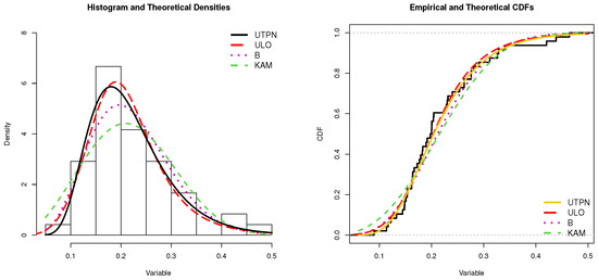
Figure 5. Models and estimated CDFs for the rock dataset.

5.2. Computation Time of P3 Algorithms

Information on the computational time of P3 algorithms, as presented in Table 5, can be found in a study by Caramanis et al. [31]. The authors of [31] used them to fit a novel statistical model that encompasses univariate and bivariate approaches. Table 6 illustrates the right-skewed nature of the dataset. Notably, the sample size is small, approximately 20, which presents a challenge for modeling. On the other side, the maximum difference between the data and the theoretical UTPN distribution, according to the K-S test results, is 0.1480. With a p-value of 0.7211, the null hypothesis, according to which the data come from the UTPN distribution, is accepted, which implies an adequate fit.

Table 5. Computational times of P3 algorithms.

0.853	0.759	0.874	0.800	0.716	0.557	0.503	0.399	0.334	0.207	0.118
0.097	0.078	0.067	0.056	0.044	0.036	0.026	0.019	0.014	0.010	0.118

Table 6. Summary statistics for the dataset on the computational duration of P3 algorithms.

Size	Mean	Variance	Skewness	Kurtosis
22	0.3039	0.3178	0.7114	1.8838

The outcomes derived from the analysis presented in Table 7 offer valuable insights into the performance of the evaluated models in capturing the underlying distribution of the P3 algorithm dataset. The test statistic D values from the K-S test are provided for each evaluated model. Notably, the UTPN model exhibits a log-likelihood value of 8.07, suggesting a favorable fit to the data. This is further supported by the information criteria (AIC, BIC, CAIC, and HQIC) consistently presenting the lowest values for the UTPN model compared to alternative models, namely the ULO, B, and KAM distributions. The parameter estimates provide nuanced understanding, with $\widehat{\alpha }$ and $\widehat{\sigma }$ shedding light on the shape and variability of the UTPN model. While uncertainty is inherent in parameter estimation, the UTPN model, characterized by $\widehat{\alpha }=0.287$ and $\widehat{\sigma }=2.177$, emerges as a promising candidate for effectively modeling data within the (0, 1) interval.

Table 7. Model parameter estimates, log-likelihood values, and goodness-of-fit measures for the P3 algorithms dataset.

Models	Estimation (SE)	$\log \left(\mathit{L}\right)$	AIC	BIC	CAIC	HQIC	K-S
UTPN	$\widehat{\alpha }=0.287\left(0.848\right)$	8.07	−12.15	−9.96	−11.51	−11.63	0.15
	$\widehat{\sigma }=2.177\left(0.806\right)$
ULO	$\widehat{\mu }=0.177\left(0.068\right)$	7.71	−11.42	−9.24	−10.79	−10.91	0.14
	$\widehat{\beta }=0.817\left(0.141\right)$
B	$\widehat{\alpha }=0.554\left(0.142\right)$	6.78	−9.56	−7.38	−8.93	−9.05	0.20
	$\widehat{\beta }=1.220\left(0.376\right)$
KAM	$\widehat{\alpha }=0.572\left(0.148\right)$	6.84	−9.69	−7.51	−9.06	−9.17	0.20
	$\widehat{\beta }=1.231\left(0.348\right)$

Graphically, Figure 6 clearly demonstrates that the UTPN distribution exhibits the most favorable performance. The figure showcases a histogram overlaid with the fitted density function, alongside a plot illustrating the empirical distribution with the estimated CDF of these fitted distributions.

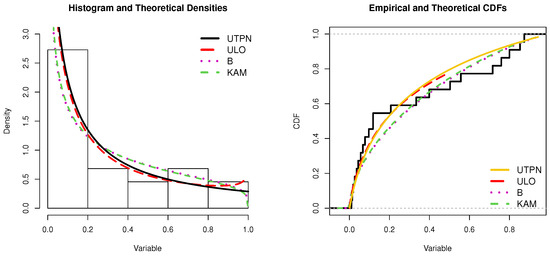
Figure 6. Models and estimated CDFs for P3 algorithms dataset.

6. Conclusions

In numerous applied scientific fields, various metrics, such as indicators, percentages, proportions, ratios, and rates, measured on the scale of (0, 1) serve as crucial study variables for characterizing diverse phenomena. However, the current statistical literature offers limited model options for handling these variables. The beta and Kumaraswamy distributions are two of the main models. This study introduces a flexible two-parameter probability distribution with a bounded domain, derived using an exponential transformation of a truncated positive normal variable, this transformation provides statistical properties related to the distribution in simple and closed form. We investigate several statistical properties of the proposed distribution, including maximum likelihood analyses conducted on two practical datasets. Notably, the obtained findings demonstrate that the proposed distribution exhibits greater flexibility compared to commonly used statistical distributions, such as beta, Kumaraswamy, and unit-logistic distributions. Particularly in the realm of modeling small samples, the obtained results underscore the superior performance of the UTPN distribution. On the other hand, the study’s findings suggest that the UTPN distribution may not be ideal for modeling lifetime data with a decreasing HR function or a bathtub-shaped HR, which includes burn-in and wear-out phases along with extended periods of low, constant hazard. Therefore, further research may aim to improve the distribution to overcome these limitations. Moreover, future research avenues could explore the derivation of alternative models from the TPN distribution using different transformations, as well as the examination of the proposed model within the quantile regression framework.

References

- Gómez, H.J.; Olmos, N.M.; Varela, H.H.; Bolfarine, H. Inference for a truncated positive normal distribution. Appl. Math. J. Chin. Univ. Ser. B 2018, 33, 163–176. [Google Scholar] [CrossRef]
- Topp, C.W.; Leone, F.C. A family of J-shaped frequency functions. J. Am. Stat. Assoc. 1955, 50, 209–219. [Google Scholar] [CrossRef]
- Grassia, A. On a family of distributions with argument between 0 and 1 obtained by transformation of the gamma and derived compound distributions. Aust. J. Stat. 1977, 19, 108–114. [Google Scholar] [CrossRef]
- Gómez-Déniz, E.; Sordo, M.A.; Calderín-Ojeda, E. The log-Lindley distribution as an alternative to the beta regression model with applications in insurance. Insur. Math. Econ. 2013, 54, 49–57. [Google Scholar] [CrossRef]
- Menezes, A.F.B.; Mazucheli, J.; Dey, S. The unit-logistic distribution: Different methods of estimation. Braz. Oper. Res. Soc. 2018, 38, 555–578. [Google Scholar] [CrossRef]
- Mazucheli, J.; Menezes, A.F.B.; Dey, S. The unit-birnbaum-saunders distribution with applications. Chil. J. Stat. 2018, 9, 47–57. [Google Scholar]
- Mazucheli, J.; Menezes, A.F.B.; Fernandes, L.B.; de Oliveira, R.P.; Ghitany, M.E. The unit-Weibull distribution as an alternative to the Kumaraswamy distribution for the dodeling of quantiles conditional on covariates. J. Appl. Stat. 2020, 47, 954–974. [Google Scholar] [CrossRef] [PubMed]
- Mazucheli, J.; Menezes, A.F.; Dey, S. Unit-Gompertz distribution with applications. Statistica 2019, 79, 25–43. [Google Scholar]
- Ghitany, M.E.; Mazucheli, J.; Menezes, A.F.B.; Alqallaf, F. The unit-inverse Gaussian distribution: A new alternative to two-parameter distributions on the unit interval. Commun. Stat. Theory Methods 2019, 48, 3423–3438. [Google Scholar] [CrossRef]
- Haq, M.A.; Hashmi, S.; Aidi, K.; Ramos, P.L.; Louzada, F. Unit modified Burr-III distribution: Estimation, characterizations and validation test. Ann. Data Sci. 2020, 10, 415–440. [Google Scholar] [CrossRef]
- Mazucheli, J.; Menezes, A.F.B.; Chakraborty, S. On the one parameter unit-Lindley distribution and its sssociated regression model for proportion data. J. Appl. Stat. 2019, 46, 700–714. [Google Scholar] [CrossRef]
- Concha-Aracena, M.S.; Barrios-Blanco, L.; Elal-Olivero, D.; Ferreira da Silva, P.H.; Nascimento, D.C.D. Extending normality: A case of unit distribution generated from the moments of the standard normal distribution. Axioms 2022, 11, 666. [Google Scholar] [CrossRef]
- Alvarez, P.I.; Varela, H.; Cortés, I.E.; Venegas, O.; Gómez, H.W. Modified unit-half-normal distribution with applications. Mathematics 2023, 12, 136. [Google Scholar] [CrossRef]
- Bakouch, H.S.; Nik, A.S.; Asgharzadeh, A.; Salinas, H.S. A flexible probability model for proportion data: Unit-half-normal distribution. Commun. Stat. Case Stud. Data Anal. Appl. 2021, 7, 271–288. [Google Scholar] [CrossRef]
- Bakouch, H.S.; Hussain, T.; Tošić, M.; Stojanović, V.S.; Qarmalah, N. Unit exponential probability distribution: Characterization and applications in environmental and engineering data modeling. Mathematics 2023, 11, 4207. [Google Scholar] [CrossRef]
- Okorie, I.E.; Afuecheta, E.; Bakouch, H.S. Unit upper truncated Weibull distribution with extension to 0 and 1 inflated model—Theory and applications. Heliyon 2023, 9, e22260. [Google Scholar] [CrossRef] [PubMed]
- Glänzel, W. A characterization theorem based on truncated moments and its application to some distribution families. In Mathematical Statistics and Probability Theory; Bauer, P., Konecny, F., Wertz, W., Eds.; Springer: Dordrecht, The Netherlands, 1987; pp. 75–84. [Google Scholar]
- Glänzel, W. A characterization of the normal distribution. Stud. Sci. Math. Hung. 1988, 2, 89–91. [Google Scholar]
- Hamedani, G.G. Characterizations of Cauchy, normal, and uniform distributions. Stud. Sci. Math. Hung. 1993, 3, 243–248. [Google Scholar]
- Akhila, P.; Girish Babu, M.; Bakouch, H.S. A versatile probabilistic model based on Yun-G family of distributions and its applications in engineering sector. J. Kerala Stat. Assoc. 2023, 34, 52–83. [Google Scholar]
- Glaser, R.E. Bathtub and related failure rate characterization. J. Am. Stat. Assoc 1980, 75, 667–672. [Google Scholar] [CrossRef]
- Bonferroni, C.E. Elementi di Statistica Generale; Seeber: Firenze, Italy, 1930. [Google Scholar]
- Rényi, A. On measures of information and entropy. In 4th Berkeley Symposium on Mathematical Statistics and Probability; Neymann, J., Ed.; University of California Press: Berkeley, CA, USA, 1961; pp. 547–561. [Google Scholar]
- Shannon, C.E. A mathematical theory of communication. Bell Syst. Tech. J. 1948, 27, 379–423. [Google Scholar] [CrossRef]
- Casella, G.; Berger, R.L. Statistical Inference; Duxbury Advanced Series Thomson Learning: Pacific Grove, CA, USA, 2002. [Google Scholar]
- Popović, B.V.; Ristić, M.M.; Cordeiro, G.M. A two-parameter distribution obtained by compounding the generalized exponential and exponential distributions. Mediterr. J. Math 2016, 13, 2935–2949. [Google Scholar] [CrossRef]
- Alomair, G.; Akdoğan, Y.; Bakouch, H.S.; Erbayram, T. On the maximum likelihood estimators’ uniqueness and existence for two unitary distributions: Analytically and graphically, with application. Symmetry 2024, 16, 610. [Google Scholar] [CrossRef]
- R Core Team. R: A Language and Environment for Statistical Computing; R Foundation for Statistical Computing: Vienna, Austria, 2024; Available online: https://www.R-project.org/ (accessed on 10 January 2024).
- Kumaraswamy, P. A generalized probability density function for double-bounded random processes. J. Hydrol. 1980, 46, 79–88. [Google Scholar] [CrossRef]
- Johnson, N.L.; Kotz, S.; Balakrishnan, N. Continuous Univariate Distributions, 2nd ed.; Chapter 25: Beta Distributions; Wiley: Hoboken, NJ, USA, 1955; Volume 2. [Google Scholar]
- Caramanis, M.; Stremel, J.; Fleck, W.; Daniel, S. Probabilistic production costing: An investigation of alternative algorithms. Int. J. Electr. Power Energy Syst. 1983, 5, 75–86. [Google Scholar] [CrossRef]
Disclaimer/Publisher’s Note: The statements, opinions and data contained in all publications are solely those of the individual author(s) and contributor(s) and not of MDPI and/or the editor(s). MDPI and/or the editor(s) disclaim responsibility for any injury to people or property resulting from any ideas, methods, instructions or products referred to in the content. |
© 2024 by the authors. Licensee MDPI, Basel, Switzerland. This article is an open access article distributed under the terms and conditions of the Creative Commons Attribution (CC BY) license (https://creativecommons.org/licenses/by/4.0/).