Bivariate Random Coefficient Integer-Valued Autoregressive Model Based on a ρ-Thinning Operator

Abstract

While overdispersion is a common phenomenon in univariate count time series data, its exploration within bivariate contexts remains limited. To fill this gap, we propose a bivariate integer-valued autoregressive model. The model leverages a modified binomial thinning operator with a dispersion parameter $\rho$ and integrates random coefficients. This approach combines characteristics from both binomial and negative binomial thinning operators, thereby offering a flexible framework capable of generating counting series exhibiting equidispersion, overdispersion, or underdispersion. Notably, our model includes two distinct classes of first-order bivariate geometric integer-valued autoregressive models: one class employs binomial thinning (BVGINAR(1)), and the other adopts negative binomial thinning (BVNGINAR(1)). We establish the stationarity and ergodicity of the model and estimate its parameters using a combination of the Yule–Walker (YW) and conditional maximum likelihood (CML) methods. Furthermore, Monte Carlo simulation experiments are conducted to evaluate the finite sample performances of the proposed estimators across various parameter configurations, and the Anderson-Darling (AD) test is employed to assess the asymptotic normality of the estimators under large sample sizes. Ultimately, we highlight the practical applicability of the examined model by analyzing two real-world datasets on crime counts in New South Wales (NSW) and comparing its performance with other popular overdispersed BINAR(1) models.

1. Introduction

Bivariate count data are prevalent across various scenarios and frequently represent the occurrences of two distinct events, objects, or individuals over a specific time frame. Bivariate integer-valued time series models, in particular, excel at preserving the paired relationship between two correlated count variables observed over certain time intervals. Such data arise in many fields, including guest nights in hotels and cottages [1], tick-by-tick data of two highly traded stocks [2], traffic accidents happening both in daylight and nighttime [3], the occurrence of different offenses in specific areas [4], and the counts of asymptomatic and symptomatic COVID-19 cases within considered regions.

Substantial research interest has been directed toward the analysis of bivariate integer-valued time series, particularly regarding their cross-correlated nature. One direction is to describe the correlation between series by employing different bivariate innovation distributions. For instance, [3] proposed a bivariate diagonal INAR(1) model with bivariate Poisson and bivariate negative binomial innovations. Similarly, [5] found that BINAR(1) models with Poisson–Lindley (PL) innovations outperform other competing INAR(1) models, whether based on diagonal or full coefficient matrices. Furthermore, [6] presented a bivariate full INAR(1) model, assuming a time-dependent innovation vector, where the mean of the innovation vector linearly increases with the previous population size. However, these models are all based on constant coefficients.

To introduce more flexibility into BINAR models, [7] considered inference for a bivariate random coefficient INAR(1) model with different geometric marginals. Thereafter, [8] proposed a more general bivariate diagonal random coefficient INAR(1) process (BRCINAR(1)) with dependent innovations. Moreover, [9] compared the performances of random coefficient BINAR(1) models based on the bivariate negative binomial distributions constructed in different ways with explanatory variables.

While these studies have made significant strides in enhancing BINAR(1) model flexibility through various marginal and innovation distributions, they have primarily focused on binomial thinning operators. The binomial thinning operator, initially proposed by [10], remains the most widely utilized approach in modeling integer-valued time series due to its capability of producing integer-valued results and offering strong interpretability. Denoted as “∘”, this operator is defined as follows:

$$\alpha \circ X=\sum _{i=1}^X{B}_i,$$

where $\alpha \in (0,1)$, X represents a non-negative integer-valued random variable, and $\left\{B_i\right\}$ denotes a sequence of independent and identically distributed Bernoulli random variables. Each $B_i$ has a probability $P(B_i=1)=\alpha$ and $P(B_i=0)=1-\alpha$, independent of X. Essentially, the binomial thinning operator assigns a value of either 0 or 1 to each counting random variable $B_i$, making it suitable for modeling scenarios where random events either survive or vanish after a period of observation.

However, in situations where the observed unit has the potential to generate multiple countable elements or trigger further stochastic occurrences beyond mere survival or disappearance, the Bernoulli random variable may not be the most suitable choice for constructing the counting series. For example, in the context of infectious diseases, an infected individual may not only survive or die but may also contribute to the generation of new cases. To address this limitation, [11] introduced the negative binomial thinning operator, defined as:

$$\alpha \ast X=\sum _{i=1}^X{G}_i,$$

where $\alpha \in (0,1)$, and $\left\{G_i\right\}$ represents a sequence of independent and identically distributed geometric random variables with a mean of $\alpha$, also independent of X.

In fact, while there are many other thinning operators proven useful in univariate integer-valued time series [12,13], the literature on different operators applied to bivariate data is limited. As far as we know, a study by [14] constructed a BINAR(1) model based on the signed thinning operator, which is capable of accommodating data with negative observations. In addition, another study by [15] proposed a new BINAR(1) model that extended the negative binomial thinning operator.

The aim of this paper is to introduce a more sophisticated $\rho$-binomial thinning operator [12] to bivariate integer-valued time series and explore statistical inference of the proposed model. The motivation behind this endeavor lies in the remarkable versatility exhibited by the counting series derived from this thinning operator. Specifically, this thinning operator enables us to describe equidispersion, overdispersion, or underdispersion characteristics concurrently within both the counting processes. Consequently, the $\rho$-thinning operator extends the capabilities of the binomial thinning [10] and negative binomial thinning operators [16], offering superior fitting capabilities to paired count data.

The outline of the paper is structured as follows. In Section 2, we introduce a definition of the $\rho$-BVGINAR(1) model and discuss the basic properties of the thinning operator for bivariate vectors. The properties of the model are further examined in Section 3. Section 4 estimates the model parameters by integrating the Yule–Walker (YW) and maximum likelihood (CML) methods, followed by simulation studies to explore the asymptotic properties of the estimators under various parameter combinations. Moreover, the Anderson-Darling (AD) test is also performed to assess the asymptotic normality of the estimators under large sample sizes. Section 5 illustrates the application of the proposed models to two real-world datasets of crime counts in New South Wales. We examine datasets with varying levels of overdispersion indices and compare the performance of our models with other bivariate integer-valued models. Finally, Section 6 provides concluding remarks and an outlook for future research. Some proofs and figures are provided in the Appendix for reference.

2. Construction of the Model

Ref. [17] introduced a novel variant of the Bernoulli distribution, termed an inflated-parameter Bernoulli (IBe) distribution, designed to model univariate count data exhibiting overdispersion. This distribution incorporates an additional parameter, $\rho$, allowing for more flexible dispersion indices. The probability mass function (pmf) for the IBe distribution is defined as follows:

$$Pr(W=w)=\left\{\begin{array}{cc}1-\alpha ,\hfill & w=0,\hfill \\ \alpha {\left(\frac{\rho }{1+\rho }\right)}^{w-1}\left(\frac{1}{1+\rho }\right),\hfill & w\in \{1,2,\dots \},\hfill \end{array}\right.$$

(1)

where $\alpha \in [0,1]$ and $\rho \in [0,1)$. The distribution can be denoted as $W\sim \mathrm{IBe}(\alpha ,\rho )$. The mean, variance, and probability generating function (pgf) of the IBe distribution are detailed below:

$$\begin{array}{cc}\hfill \mathrm{E}\left(W\right)=& \alpha (1+\rho ),\hfill \\ \hfill \mathrm{Var}\left(W\right)=& \alpha (1+\rho )\left[\right(1+2\rho )-\alpha (1+\rho \left)\right],\hfill \\ \hfill {\Phi }_W\left(s\right)=& \frac{1-(1-s)\left[\alpha \right(1+\rho )-\rho ]}{1+\rho (1-s)},\left|s\right|<1.\hfill \end{array}$$

Moreover, the dispersion index is expressed as:

$$I_Y:=\frac{\mathrm{Var}\left(\mathrm{W}\right)}{E\left(W\right)}=\rho +(1+\rho )(1-\alpha ).$$

(2)

Interestingly, the IBe distribution presents three dispersion scenarios depending on the values of the parameters:

• Overdispersion is observed when $\frac{\alpha }{2-\alpha }<\rho <1$.
• Underdispersion occurs if $0\le \rho <\frac{\alpha }{2-\alpha }$.
• Equidispersion is achieved at $\rho =\frac{\alpha }{2-\alpha }$.

The distribution can also degenerate into two important distributions:

• The standard Bernoulli distribution, when $\rho =0$ and $w\in \{0,1\}$, with mean $\alpha$;
• The geometric distribution, when $\alpha =\frac{\rho }{1+\rho }$, with mean $\rho$.

Inspired by these properties, [12] formulated a $\rho$-binomial thinning operator, defined as:

$${\alpha }_{\rho }\circ X:=\sum _{i=1}^X{W}_i,$$

(3)

where X is a non-negative integer-valued random variable, and ${\left\{W_i\right\}}_{i=1}^X$ is a sequence of inflated-parameter Bernoulli random variables with the pmf given by Equation (1), mutually independent of X. This operator has proven its practical utility in modeling univariate integer-valued time series, known as the $\rho$-GINAR process.

However, it is crucial to acknowledge that cross-correlations are prevalent in most paired count time series. Hence, this paper aims to enhance the $\rho$-GINAR process by extending it into a bivariate domain, thereby more effectively capturing the inherent correlations within the data.

We propose the $\rho$-BVGINAR(1) model, which is a novel bivariate random coefficient INAR(1) process characterized by the following recursive equation:

$${\mathit{X}}_t={{\mathit{A}}_t}_{\rho }\circ {\mathit{X}}_{t-1}+{\mathit{Z}}_t=\left[\begin{array}{cc}{U}_{1,t}& U_{2,t}\\ V_{1,t}& V_{2,t}\end{array}\right]{ }_{\rho }\circ \left[\begin{array}{c}{X}_{1,t-1}\\ X_{2,t-1}\end{array}\right]+\left[\begin{array}{c}{Z}_{1,t}\\ Z_{2,t}\end{array}\right].$$

(4)

Here,

(i)

${\mathit{A}}_t$ represents a random coefficient matrix comprising two mutually independent bivariate random vectors, $(U_{1,t},U_{2,t})$ and $(V_{1,t},V_{2,t})$, each with independent and identically distributed (i.i.d.) components and with pmf values as:

$$P(U_{1,t}={\alpha }_1,U_{2,t}=0)=1-P(U_{1,t}=0,U_{2,t}={\alpha }_1)=p_1,$$

$$P(V_{1,t}={\alpha }_2,V_{2,t}=0)=1-P(V_{1,t}=0,V_{2,t}={\alpha }_2)=p_2,$$

where ${\alpha }_1,{\alpha }_2\in (0,1)$ and $p_1,p_2\in [0,1]$. The matrix operation ${{\mathit{A}}_t}_{\rho }\circ$ replicates matrix multiplication while preserving the properties of random coefficient thinning.

(ii)

The innovation ${\left\{{\mathit{Z}}_t\right\}}_{t\in \mathbb{Z}}$ is a sequence of i.i.d. bivariate non-negative integer-valued random vectors with mutually independent elements $\left\{Z_{1,t}\right\}$ and $\left\{Z_{2,t}\right\}$ and independent of ${\mathit{X}}_s$ for $s<t$.

Remark 1. 

The proposed bivariate INAR(1) process based on the ρ-binomial thinning operator has two sub-models:

• When $\rho =0$, it corresponds to the bivariate INAR(1) with geometric marginals introduced by [4].
• When ${\alpha }_i=\frac{\rho }{1+\rho }$, for both $i=1$ and $i=2$, it aligns with the BVNGINAR(1) proposed by [18].

Next, we further explore the properties of the $\rho$-thinning operator for vectors.

Lemma 1. 

Consider ${{\mathit{A}}_t}_{\rho }\circ {\mathit{X}}_{t-1}$ as defined in Equation (4). Then:

(i) 

$E({{\mathit{A}}_t}_{\rho }\circ {\mathit{X}}_{t-1})=\tilde{\mathit{A}}E\left({\mathit{X}}_{t-1}\right)$, where

$$\tilde{\mathit{A}}=(1+\rho )\mathit{A}=(1+\rho )E\left({\mathit{A}}_t\right)=(1+\rho )\left[\begin{array}{cc}{\alpha }_1{p}_1& {\alpha }_1(1-p_1)\\ {\alpha }_2{p}_2& {\alpha }_2(1-p_2)\end{array}\right].$$

(ii) 

$E\left(({{\mathit{A}}_t}_{\rho }\circ {\mathit{X}}_{t-1}){\mathit{B}}^{\top }\right)=\tilde{\mathit{A}}E\left({\mathit{X}}_{t-1}{\mathit{B}}^{\top }\right)$ for a random vector $\mathit{B}$ independent of ${\mathit{A}}_t$.

(iii) 

$E\left(\mathit{B}{({{\mathit{A}}_t}_{\rho }\circ {\mathit{X}}_{t-1})}^{\top }\right)=E\left(\mathit{B}{\mathit{X}}_{t-1}^{\top }\right){\tilde{\mathit{A}}}^{\top }$ for a random vector $\mathit{B}$ independent of ${\mathit{A}}_t$.

(iv) 

$E\left(({{\mathit{A}}_t}_{\rho }\circ {\mathit{X}}_{t-1}){({{\mathit{A}}_t}_{\rho }\circ {\mathit{X}}_{t-1})}^{\top }\right)=\tilde{\mathit{A}}E\left({\mathit{X}}_{t-1}{\mathit{X}}_{t-1}^{\top }\right){\tilde{\mathit{A}}}^{\top }+\mathit{C}$, where $\mathit{C}$ has elements

$$c_{12}=0,c_{21}=0,$$

$$c_{11}={(1+\rho )}^2{\alpha }_1^{2}p(1-p_1)E{(X_{1,t}-X_{2,t})}^2+{\alpha }_1(1+\rho )(1+2\rho -{\alpha }_1(1+p_1))(p_{1}E\left(X_{1,t}\right)+(1-p_1)E\left(X_{2,t}\right))),$$

$$c_{22}={(1+\rho )}^2{\alpha }_2^2{p}_2(1-p_2)E{(X_{1,t}-X_{2,t})}^2+{\alpha }_2(1+\rho )(1+2\rho -{\alpha }_2(1+p_2))(p_{2}E\left(X_{1,t}\right)+(1-p_2)E\left(X_{2,t}\right))).$$

Lemma 2. 

If we assume ${\alpha }_1(1+\rho ),{\alpha }_2(1+\rho )\in (0,1)$, then all eigenvalues of matrix $\tilde{\mathit{A}}$ lie within the unit circle.

Proof. 

Similar to [19], we outline the key steps. Let ${\lambda }_1$ and ${\lambda }_2$ denote the eigenvalues, with ${\lambda }_2>{\lambda }_1$ assumed without loss of generality.

(i)

We have ${\lambda }_1+{\lambda }_2=(1+\rho ){\alpha }_1{p}_1+(1+\rho ){\alpha }_2(1-p_2)>0$, indicating ${\lambda }_2>0$.

(ii)

Furthermore, we calculate ${\lambda }_1{\lambda }_2={(1+\rho )}^2{\alpha }_1{p}_1{\alpha }_2(1-q_1)-{(1+\rho )}^2{\alpha }_1(1-p_1){\alpha }_2{p}_2$; then, we have $(1-{\lambda }_1)(1-{\lambda }_2)=1-({\lambda }_1+{\lambda }_2)+{\lambda }_1{\lambda }_2=(1-(1+\rho ){\alpha }_1{p}_1)(1-(1+\rho ){\alpha }_2(1-p_2))-{(1+\rho )}^2{\alpha }_1(1-p_1){\alpha }_2{p}_2\ge (1-p_1)(1-(1-p_2))-(1-p_1)p_2=0.$ Hence, it necessitates that either both ${\lambda }_1,{\lambda }_2<1$ or both ${\lambda }_1,{\lambda }_2>1$. Since ${\lambda }_1+{\lambda }_2=(1+\rho ){\alpha }_1{p}_1+(1+\rho ){\alpha }_2(1-p_2)<2$, we deduce both ${\lambda }_1,{\lambda }_2<1$.

(iii)

Similarly, evaluating $(1+{\lambda }_1)(1+{\lambda }_2)=1+({\lambda }_1+{\lambda }_2)+{\lambda }_1{\lambda }_2=(1+(1+\rho ){\alpha }_1{p}_1)(1+(1+\rho ){\alpha }_2(1-p_2))-{(1+\rho )}^2{\alpha }_1(1-p_1){\alpha }_2{p}_2>0$. As ${\lambda }_2>0$, then ${\lambda }_1<-1$.

Consequently, we conclude $-1<{\lambda }_1<1$ and $0<{\lambda }_2<1$ under the conditions ${\alpha }_1(1+\rho ),{\alpha }_2(1+\rho )\in (0,1)$. Moreover, this condition ensures the stationarity of both the first- and second-order moments of the process. □

Proposition 1. 

If ${\alpha }_1(1+\rho ),{\alpha }_2(1+\rho )\in (0,1)$ and $p_1,p_2\in [0,1]$, a strictly stationary bivariate integer-valued time series ${\left\{{\mathit{X}}_t\right\}}_{t\in \mathbb{Z}}$ satisfying Equation (4) exists uniquely. Moreover, the process is ergodic.

The proof of Proposition 1 is provided in Appendix B. Now let us derive the moments and conditional moments of the $\rho$-BVGINAR(1) process.

Proposition 2. 

Suppose the bivariate time series ${\left\{{\mathit{X}}_t\right\}}_{\{t\in \mathbb{Z}\}}$ is a stationary process defined by Equation (4); then, for $t\ge 1,i=1,2$, we have

(i) 

$E\left({\mathit{X}}_t\right)={(\mathit{I}-\tilde{\mathit{A}})}^{-1}E\left(\mathit{Z}\right)$.

(ii) 

${\Sigma }_{{\mathit{X}}_{\mathit{t}+\mathit{1}}}=\tilde{\mathit{A}}{\Sigma }_{{\mathit{X}}_{\mathit{t}}}{\tilde{\mathit{A}}}^{\top }+\mathit{C}+{\Sigma }_{\mathit{Z}}$, where $\mathit{C}$ has elements

$$c_{12}=0,c_{21}=0,$$

$$c_{11}={(1+\rho )}^2{\alpha }_1^{2}p(1-p_1)E{(X_{1,t}-X_{2,t})}^2+{\alpha }_1(1+\rho )(1+2\rho -{\alpha }_1(1+p_1))(p_{1}E\left(X_{1,t}\right)+(1-p_1)E\left(X_{2,t}\right))),$$

$$c_{22}={(1+\rho )}^2{\alpha }_2^2{p}_2(1-p_2)E{(X_{1,t}-X_{2,t})}^2+{\alpha }_2(1+\rho )(1+2\rho -{\alpha }_2(1+p_2))(p_{2}E\left(X_{1,t}\right)+(1-p_2)E\left(X_{2,t}\right))).$$

(iii) 

$E\left(X_{i,t+1}\right|X_{1,t},X_{2,t})=(1+\rho ){\alpha }_i[p_i{X}_{1,t}+(1-p_i)X_{2,t}]+{\mu }_{Z_{i,t}}$.

(iv) 

$\mathrm{Var}\left(X_{i,t+1}\right|X_{1,t},X_{2,t})={(1+\rho )}^2{\alpha }_i^2{p}_i(1-p_i)(X_{1,t}^2+X_{2,t}^2)+(1+\rho )[1+2\rho -(1+\rho ){\alpha }_i]{\alpha }_i$$[p_i{X}_{1,t}+(1-p_i)X_{2,t}]-2{(1+\rho )}^2{\alpha }_i^2{p}_i(1-p_i)X_{1,t}{X}_{2,t}+{\sigma }_{Z_{i,t}}^2.$

where ${\mu }_{Z_{i,t}}$ and ${\sigma }_{Z_{i,t}}^2$ are the mean and variance, respectively, of $\left\{Z_{i,t}\right\}$, for $i=1,2$.

We define a stationary bivariate time series ${(X_{1,t},X_{2,t})}_{t\in \mathbb{Z}}$ according to Equation (4). By specifying appropriate marginal distributions for $X_{1,t}$ and $X_{2,t}$, we can deduce the respective marginal distributions of the innovation $Z_{1,t}$ and $Z_{2,t}$. This process is clarified by the theorem below.

Theorem 1. 

Let ${\alpha }_1(1+\rho ),{\alpha }_2(1+\rho )\in (0,1)$, $p_1,p_2\in [0,1]$ if $\left\{X_{1,t}\right\}\stackrel{d}{=}\left\{X_{2,t}\right\}\stackrel{d}{=}Geom\left(\frac{\mu }{1+\mu }\right)$, and $\mu >0$; then the distributions of the innovation processes $\left\{Z_{1,t}\right\}$ and $\left\{Z_{2,t}\right\}$ are as follows:

$$Z_{1,t}\stackrel{d}{=}\left\{\begin{array}{c}Geom\left(\frac{\rho }{1+\rho }\right),\mathrm{w}.\mathrm{p}.\frac{{\alpha }_1\mu (1+\rho )}{\mu -\rho },\hfill \\ Geom\left(\frac{\mu }{1+\mu }\right),\mathrm{w}.\mathrm{p}.1-\frac{{\alpha }_1\mu (1+\rho )}{\mu -\rho },\hfill \end{array}\right.$$

(5)

$$Z_{2,t}\stackrel{d}{=}\left\{\begin{array}{c}Geom\left(\frac{\rho }{1+\rho }\right),\mathrm{w}.\mathrm{p}.\frac{{\alpha }_2\mu (1+\rho )}{\mu -\rho },\hfill \\ Geom\left(\frac{\mu }{1+\mu }\right),\mathrm{w}.\mathrm{p}.1-\frac{{\alpha }_2\mu (1+\rho )}{\mu -\rho }.\hfill \end{array}\right.$$

(6)

Proof. 

For intuitive purposes, the bivariate time series model ${\left\{(X_{1,t},X_{2,t})\right\}}_{t\in \mathbb{Z}}$ can be represented as

$$X_{1,t}=\left\{\begin{array}{c}{{\alpha }_1}_{\rho }\circ X_{1,t-1}+Z_{1,t},\mathrm{w}.\mathrm{p}.p_1,\hfill \\ {{\alpha }_1}_{\rho }\circ X_{2,t-1}+Z_{1,t},\mathrm{w}.\mathrm{p}.1-p_1,\hfill \end{array}\right.$$

$$X_{2,t}=\left\{\begin{array}{c}{{\alpha }_2}_{\rho }\circ X_{1,t-1}+Z_{2,t},\mathrm{w}.\mathrm{p}.p_2,\hfill \\ {{\alpha }_2}_{\rho }\circ X_{2,t-1}+Z_{2,t},\mathrm{w}.\mathrm{p}.1-p_2.\hfill \end{array}\right.$$

Given $\left\{X_{1,t}\right\}\stackrel{d}{=}\left\{X_{2,t}\right\}\stackrel{d}{=}Geom\left(\frac{\mu }{1+\mu }\right)$ and leveraging the properties of the thinning operator and the stationarity of the process, we have

$$\begin{array}{cc}\hfill {\Phi }_{{{\alpha }_1}_{\rho }\circ X_{1,t}}\left(s\right)=& E\left(s^{{{\alpha }_1}_{\rho }\circ X_{1,t}}\right)\hfill \\ \hfill =& E\left[E\left(s^{{\displaystyle \sum _{j=1}^{X_{1,t}}}{W}_j({\alpha }_1,\rho )}\right|X_{1,t})\right]\hfill \\ \hfill =& E\left[E{\left(s^{W_j({\alpha }_1,\rho )}\right|X_{1,t})}^{X_{1,t}}\right]\hfill \\ \hfill =& E\left[{\left({\Phi }_W\left(s\right)\right)}^{X_{1,t}}\right]\hfill \\ \hfill =& {\Phi }_{X_{1,t}}\left({\Phi }_W\left(s\right)\right)\hfill \\ \hfill =& {\Phi }_{X_{1,t}}\left(\frac{1-(1-s)[{\alpha }_1(1+\rho )-\rho ]}{1+\rho (1-s)}\right).\hfill \end{array}$$

Then the pgf of $Z_{1,t}$ can be obtained by

$$\begin{array}{cc}\hfill {\Phi }_{Z_{1,t}}\left(s\right)=& \frac{{\Phi }_{X_{1,t}}\left(s\right)}{p_1{\Phi }_{X_{1,t}}\left({\Phi }_W\left(s\right)\right)+(1-p_1){\Phi }_{X_{1,t}}\left({\Phi }_W\left(s\right)\right)}\hfill \\ \hfill =& \frac{\frac{1}{1+\mu -\mu s}}{p_1·{\Phi }_{X_{1,t}}\left(\frac{1-(1-s)[{\alpha }_1(1+\rho )-\rho ]}{1+\rho (1-s)}\right)+(1-p_1)·{\Phi }_{X_{2,t}}\left(\frac{1-(1-s)[{\alpha }_1(1+\rho )-\rho ]}{1+\rho (1-s)}\right)}\hfill \\ \hfill =& \frac{1+\rho (1-s)+{\alpha }_1\mu (1+\rho )(1-s)}{[1+\mu (1-s\left)\right][1+\rho (1-s\left)\right]}\hfill \\ \hfill =& \frac{[1+\rho (1-s)+{\alpha }_1\mu (1+\rho )(1-s)](\mu -\rho )}{[1+\mu (1-s\left)\right][1+\rho (1-s\left)\right](\mu -\rho )}\hfill \\ \hfill =& \frac{(\mu -\rho )-{\alpha }_1\mu (1+\rho )}{(\mu -\rho )[1+\mu (1-s\left)\right]}+\frac{{\alpha }_1\mu (1+\rho )}{(\mu -\rho )[1+\rho (1-s\left)\right]}\hfill \\ \hfill =& \left(1-\frac{{\alpha }_1\mu (1+\rho )}{\mu -\rho }\right)\frac{1}{1+\mu (1-s)}+\frac{{\alpha }_1\mu (1+\rho )}{\mu -\rho }\frac{1}{1+\rho (1-s)}.\hfill \end{array}$$

The innovation $Z_{1,t}$ clearly consists of a combination of two geometrically distributed random variables. Similar derivation holds for $Z_{2,t}$. Thus, the distributions of innovation process can be expressed as Equations (5) and (6). Notably, it is emphasized that $0<\rho <min(\frac{\mu (1-{\alpha }_1)}{1+{\alpha }_1\mu },\frac{\mu (1-{\alpha }_2)}{1+{\alpha }_2\mu })$ is necessary to ensure the non-negativity of all probabilities for $Z_{1,t}$ and $Z_{2,t}$. □

3. Properties

Lemma 3. 

Let $0<\rho <min(\frac{\mu (1-{\alpha }_1)}{1+{\alpha }_1\mu },\frac{\mu (1-{\alpha }_2)}{1+{\alpha }_2\mu })$, and $p_1,p_2\in [0,1]$. The correlation coefficient between $\left\{X_{1,t}\right\}$ and $\left\{X_{2,t}\right\}$ lies in $[0,1)$ and is expressed as:

$$\gamma =\frac{{(1+\rho )}^2{\alpha }_1{\alpha }_2(p_1{p}_2+(1-p_1)(1-p_2))}{1-{(1+\rho )}^2{\alpha }_1{\alpha }_2(p_1(1-p_2)+(1-p_1)p_2)}.$$

(7)

It is evident that the correlation coefficient γ lies in the interval $[0,1)$.

From Lemma 1, we find that the covariance matrix between the random vectors ${\mathit{X}}_t$ and ${\mathit{X}}_0$ is given by

$$\mathrm{Cov}({\mathit{X}}_t,{\mathit{X}}_0)=\tilde{\mathit{A}}\mathrm{Cov}({\mathit{X}}_{t-1},{\mathit{X}}_0)=\cdots ={\tilde{\mathit{A}}}^t\mathrm{Var}\left({\mathit{X}}_0\right)\to 0,t\to \infty .$$

The one-step-ahead conditional expectation can be derived as follows:

$$\begin{array}{c}\hfill E\left({\mathit{X}}_{\mathit{t}+\mathit{1}}\right|{\mathit{X}}_{\mathit{t}})=\tilde{\mathit{A}}{\mathit{X}}_{\mathit{t}}+E\left({\mathit{Z}}_{\mathit{t}+\mathit{1}}\right).\end{array}$$

Typically, the k-step ahead conditional expectation of ${\mathit{X}}_t$ is

$$\begin{array}{cc}\hfill E\left({\mathit{X}}_{\mathit{t}}\right|{\mathit{X}}_{\mathit{t}-\mathit{k}})=& E({{\mathit{A}}_t}_{\rho }\circ {\mathit{X}}_{\mathit{t}-\mathit{1}}+{\mathit{Z}}_t|{\mathit{X}}_{\mathit{t}-\mathit{k}})\hfill \\ \hfill =& E({{\mathit{A}}_{\mathit{t}}^{\mathit{k}}}_{\rho }\circ {\mathit{X}}_{\mathit{t}-\mathit{k}}+\sum _{j=1}^{k-1}{{\mathit{A}}_{\mathit{t}}^{\mathit{j}}}_{\rho }\circ {\mathit{Z}}_{\mathit{t}-\mathit{j}}|{\mathit{X}}_{\mathit{t}-\mathit{k}})\hfill \\ \hfill =& {\tilde{\mathit{A}}}^k{\mathit{X}}_{\mathit{t}-\mathit{k}}+\sum _{j=1}^{k-1}{\left[\tilde{\mathit{A}}\right]}^{j}E\left({\mathit{Z}}_{\mathit{t}}\right)\hfill \\ \hfill =& {\tilde{\mathit{A}}}^k{\mathit{X}}_{\mathit{t}-\mathit{k}}+[\mathit{I}-{\tilde{\mathit{A}}}^k]{[\mathit{I}-\tilde{\mathit{A}}]}^{-1}E\left({\mathit{Z}}_{\mathit{t}}\right).\hfill \end{array}$$

Meanwhile, we observe that $E\left({\mathit{Z}}_{\mathit{t}}\right)=[\mathit{I}-\tilde{\mathit{A}}]E\left({\mathit{X}}_{\mathit{t}}\right)$, thereby implying that

$$E\left({\mathit{X}}_{\mathit{t}}\right|{\mathit{X}}_{\mathit{t}-\mathit{k}})={\tilde{\mathit{A}}}^k{\mathit{X}}_{\mathit{t}-\mathit{k}}+[\mathit{I}-{\tilde{\mathit{A}}}^k]E\left({\mathit{X}}_{\mathit{t}}\right)\to E\left({\mathit{X}}_{\mathit{t}}\right),k\to \infty .$$

This finding validates the characteristic of autoregressive processes, whereby the conditional expectation converges to the unconditional expectation as the number of steps approaches infinity.

Due to the conditional independence of the random variables $X_{1,t}$ and $X_{2,t}$ conditioned on $X_{1,t-1}$ and $X_{2,t-1}$, respectively, the conditional probability function can be represented as the product of individual conditional probabilities. Therefore, we can derive the conditional probability function of the random vector ${(X_{1,t},X_{2,t})}^{\top }$ as follows:

$$\begin{array}{cc}\hfill P(X_{1,t}=& x,X_{2,t}=y|X_{1,t-1}=u,X_{2,t-1}=v)=\hfill \\ \hfill P(& X_{1,t}=x|X_{1,t-1}=u,X_{2,t-1}=v)·P(X_{2,t}=y|X_{1,t-1}=u,X_{2,t-1}=v),\hfill \end{array}$$

(8)

where

$$\begin{array}{cc}\hfill P(X_{1,t}=& x|X_{1,t-1}=u,X_{2,t-1}=v)\hfill \\ \hfill =& p_1(P({{\alpha }_1}_{\rho }\circ X_{1,t-1}=0|X_{1,t-1}=u)P(Z_{1,t}=x)\hfill \\ \hfill & +\sum _{k=1}^{x}P({{\alpha }_1}_{\rho }\circ X_{1,t-1}=k|X_{1,t-1}=u)P(Z_{1,t}=x-k))\hfill \\ \hfill & +(1-p_1)(P({{\alpha }_1}_{\rho }\circ X_{2,t-1}=0|X_{2,t-1}=v)P(Z_{1,t}=x)\hfill \\ \hfill & +\sum _{k=1}^{x}P({{\alpha }_1}_{\rho }\circ X_{2,t-1}=k|X_{2,t-1}=v)P(Z_{1,t}=x-k)),\hfill \end{array}$$

(9)

and

$$\begin{array}{cc}\hfill P(X_{2,t}=& y|X_{1,t-1}=u,X_{2,t-1}=v)\hfill \\ \hfill =& p_2(P({{\alpha }_2}_{\rho }\circ X_{2,t-1}=0|X_{1,t-1}=u)P(Z_{2,t}=y)\hfill \\ \hfill & +\sum _{k=1}^{y}P({{\alpha }_2}_{\rho }\circ X_{2,t-1}=k|X_{1,t-1}=u)P(Z_{2,t}=y-k))\hfill \\ \hfill & +(1-p_2)(P({{\alpha }_2}_{\rho }\circ X_{2,t-1}=0|X_{1,t-1}=v)P(Z_{2,t}=y)\hfill \\ \hfill & +\sum _{k=1}^{y}P({{\alpha }_2}_{\rho }\circ X_{2,t-1}=k|X_{2,t-1}=v)P(Z_{2,t}=y-k)).\hfill \end{array}$$

(10)

Here, the distributions of the random variables $Z_{1,t}$ and $Z_{2,t}$ are defined by Theorem 1, so their probability mass functions are given by

$$P(Z_{1,t}=z_1)=\frac{{\mu }^{z_1}}{{(1+\mu )}^{z_1+1}}(1-\frac{{\alpha }_1\mu (1+\rho )}{\mu -\rho })+\frac{{\rho }^{z_1}}{{(1+\rho )}^{z_1+1}}\left(\frac{{\alpha }_1\mu (1+\rho )}{\mu -\rho }\right)$$

(11)

and

$$P(Z_{2,t}=z_2)=\frac{{\mu }^{z_2}}{{(1+\mu )}^{z_2+1}}(1-\frac{{\alpha }_2\mu (1+\rho )}{\mu -\rho })+\frac{{\rho }^{z_2}}{{(1+\rho )}^{z_2+1}}\left(\frac{{\alpha }_2\mu (1+\rho )}{\mu -\rho }\right).$$

(12)

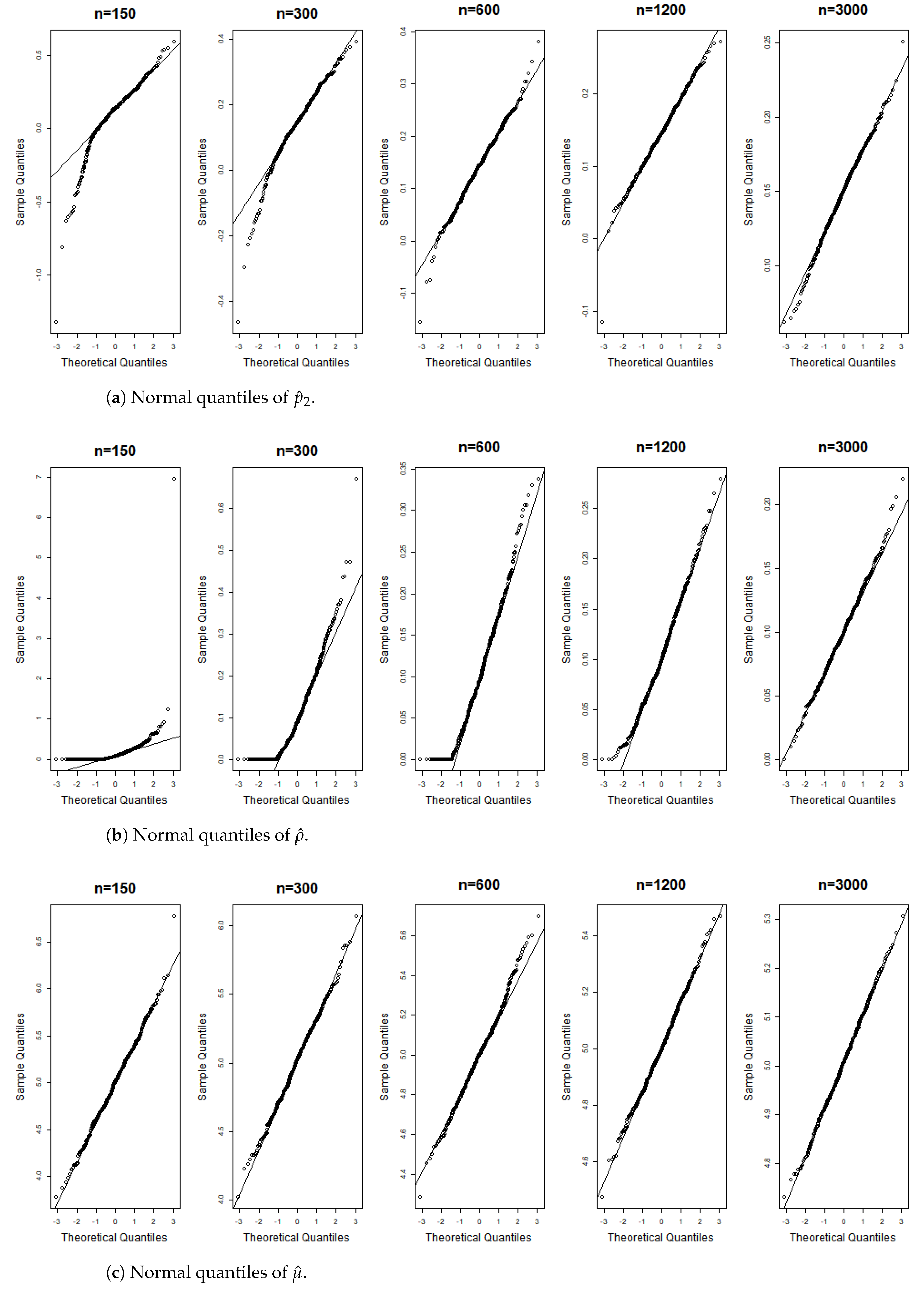
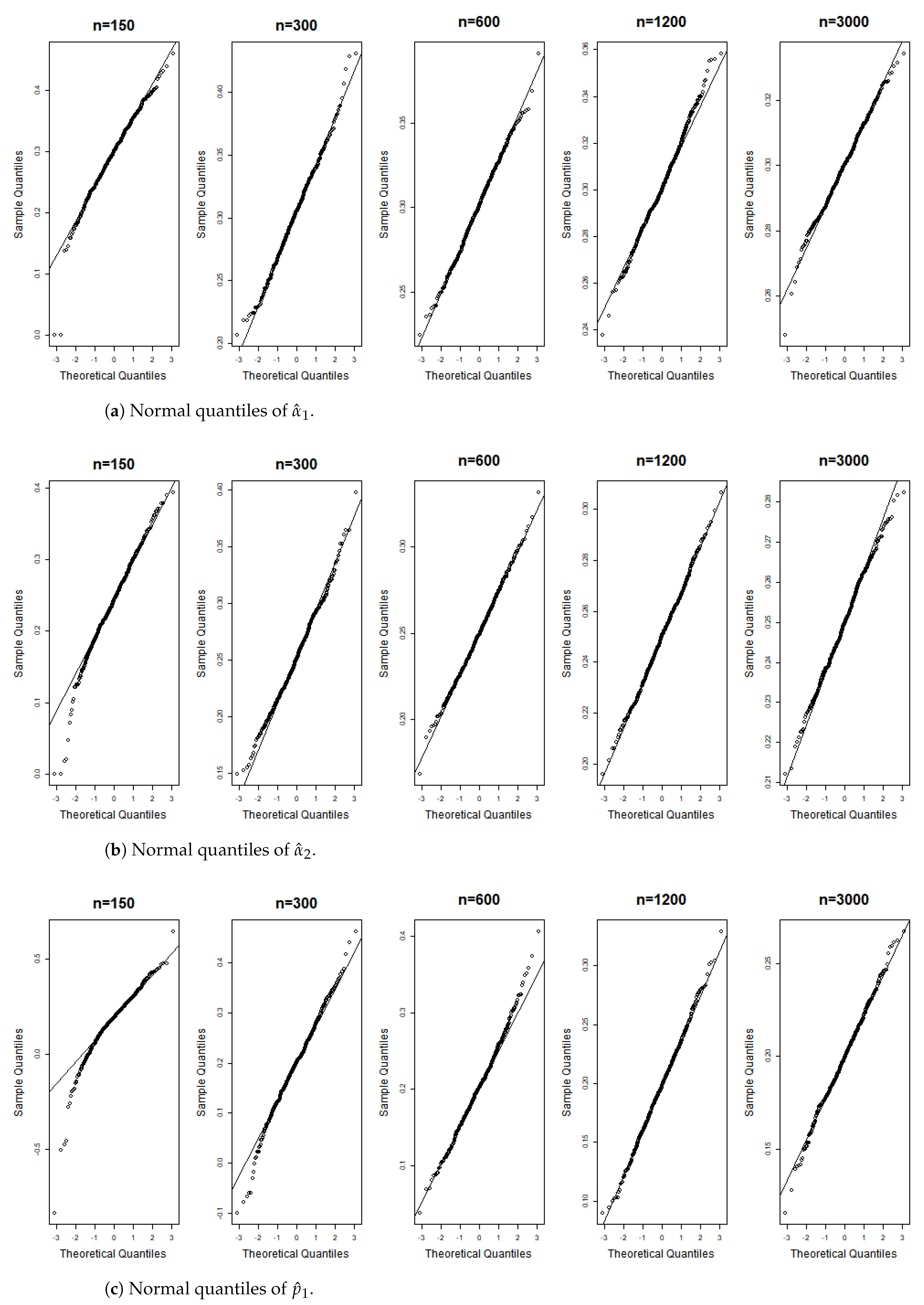
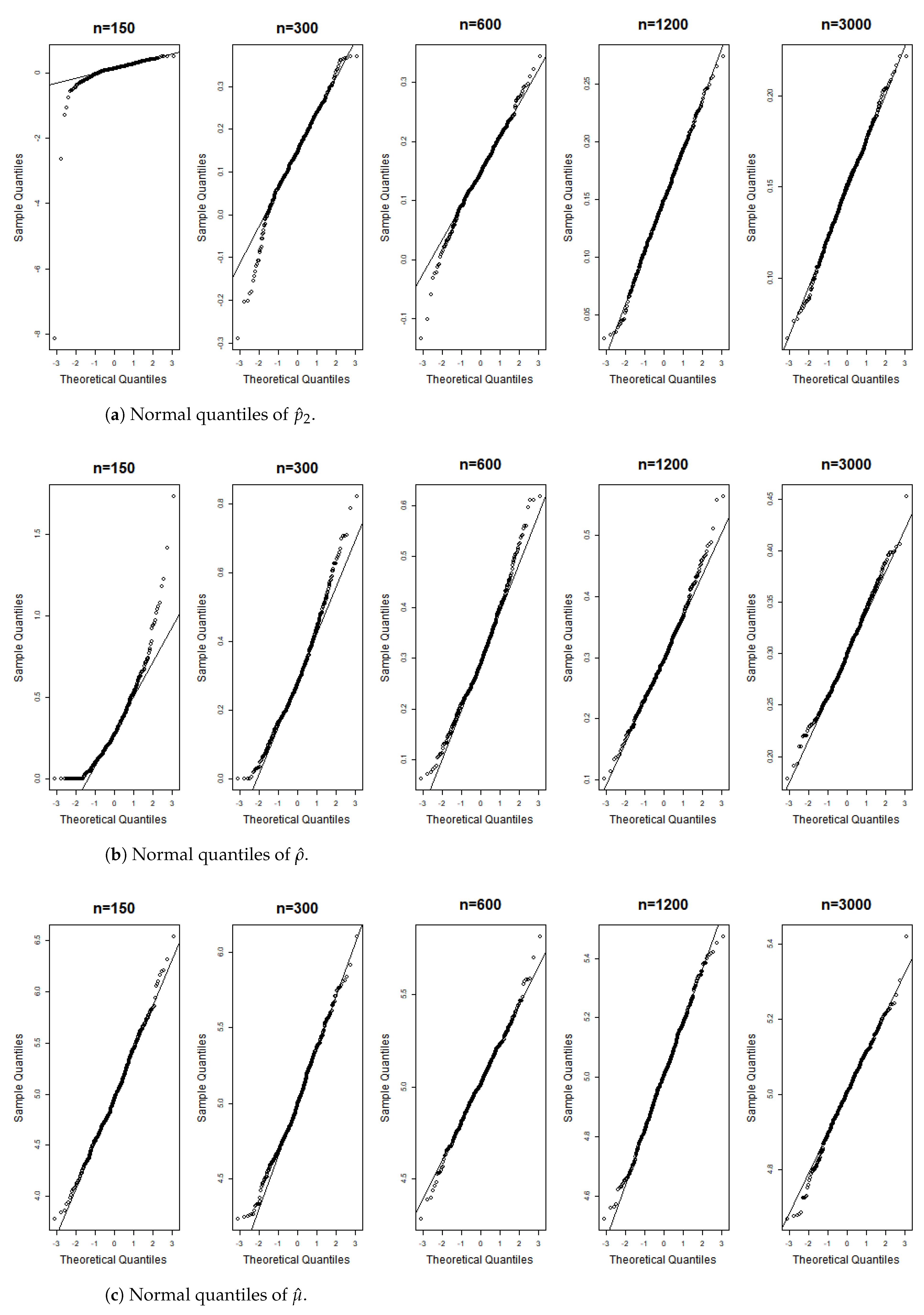
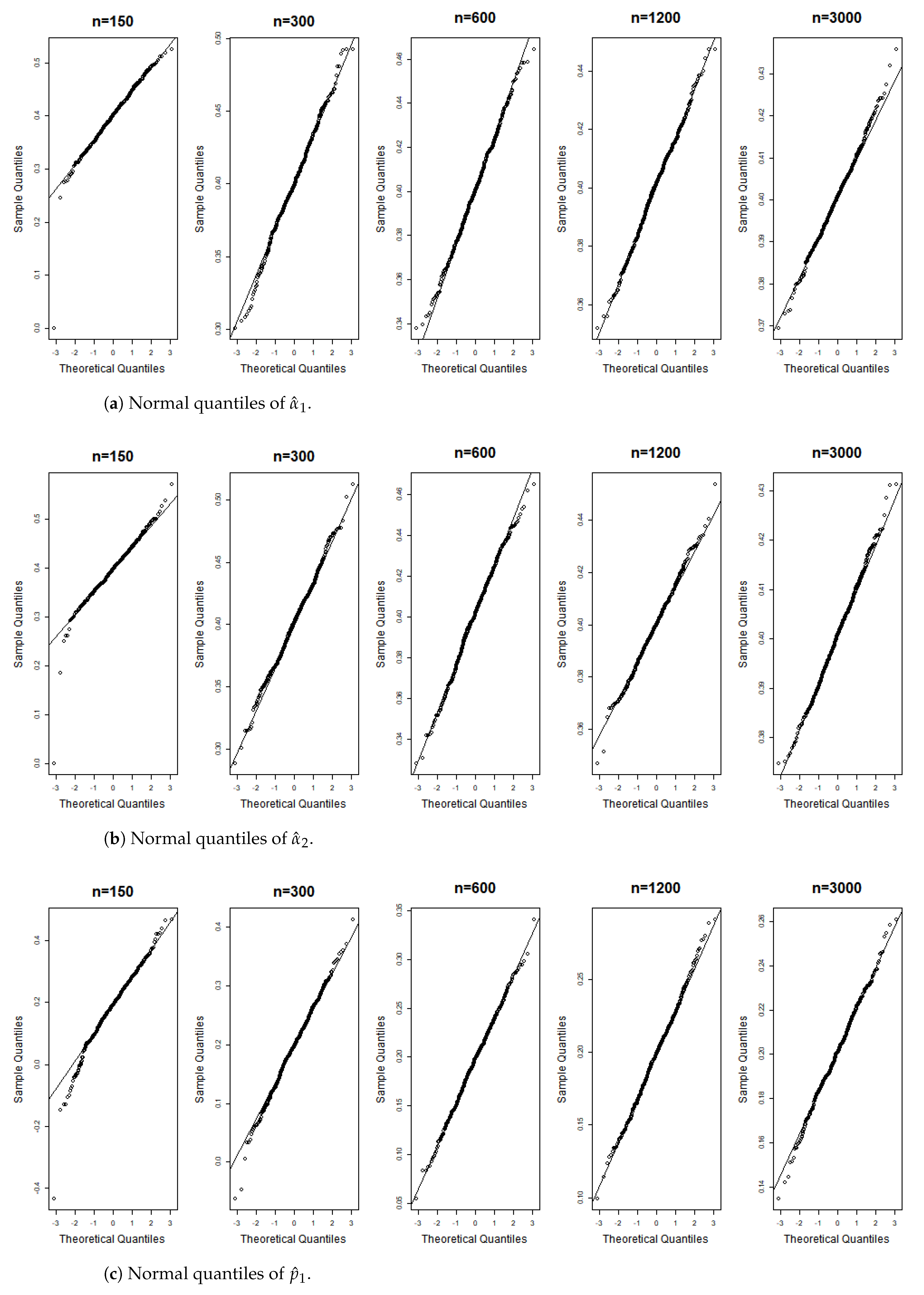
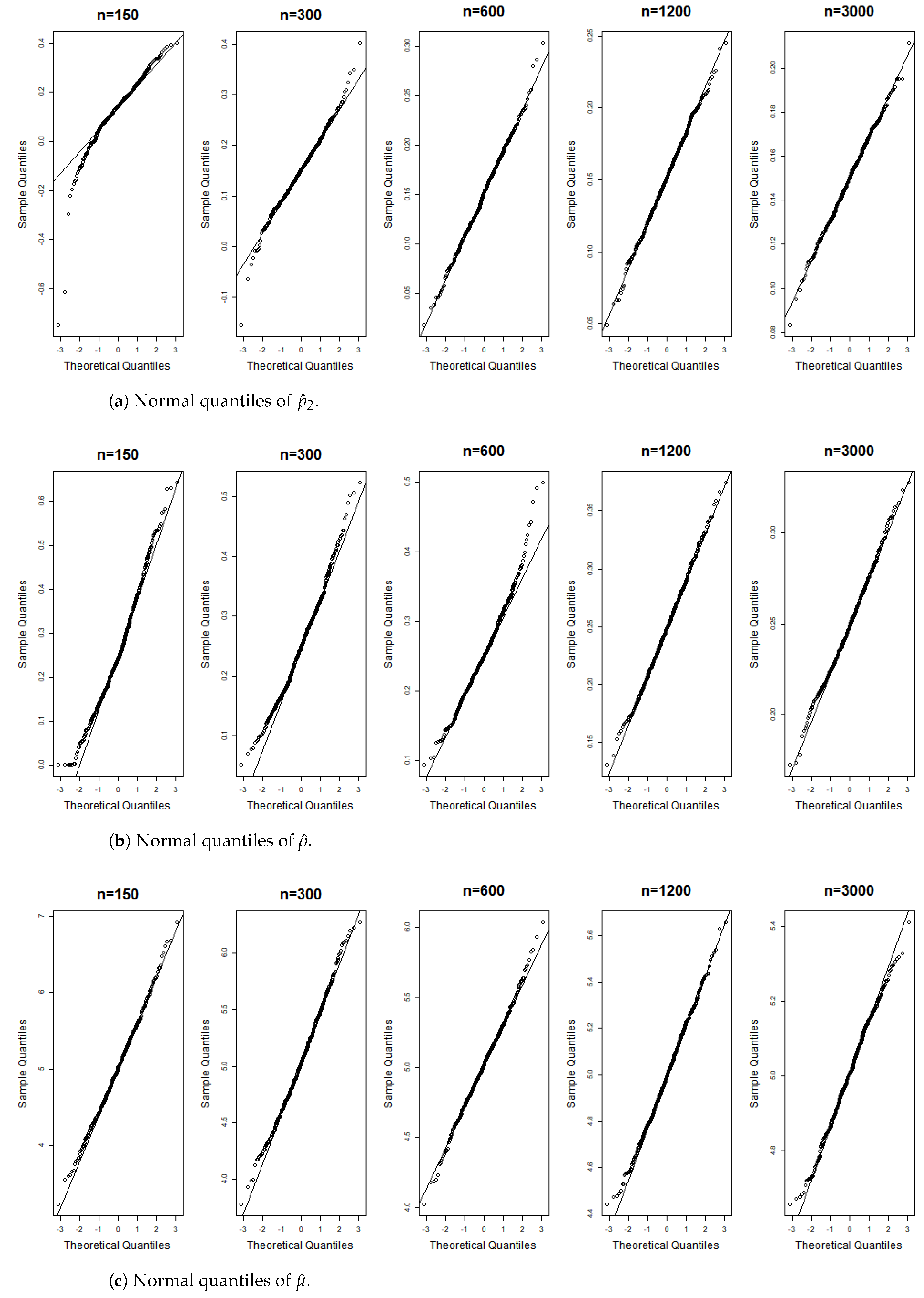
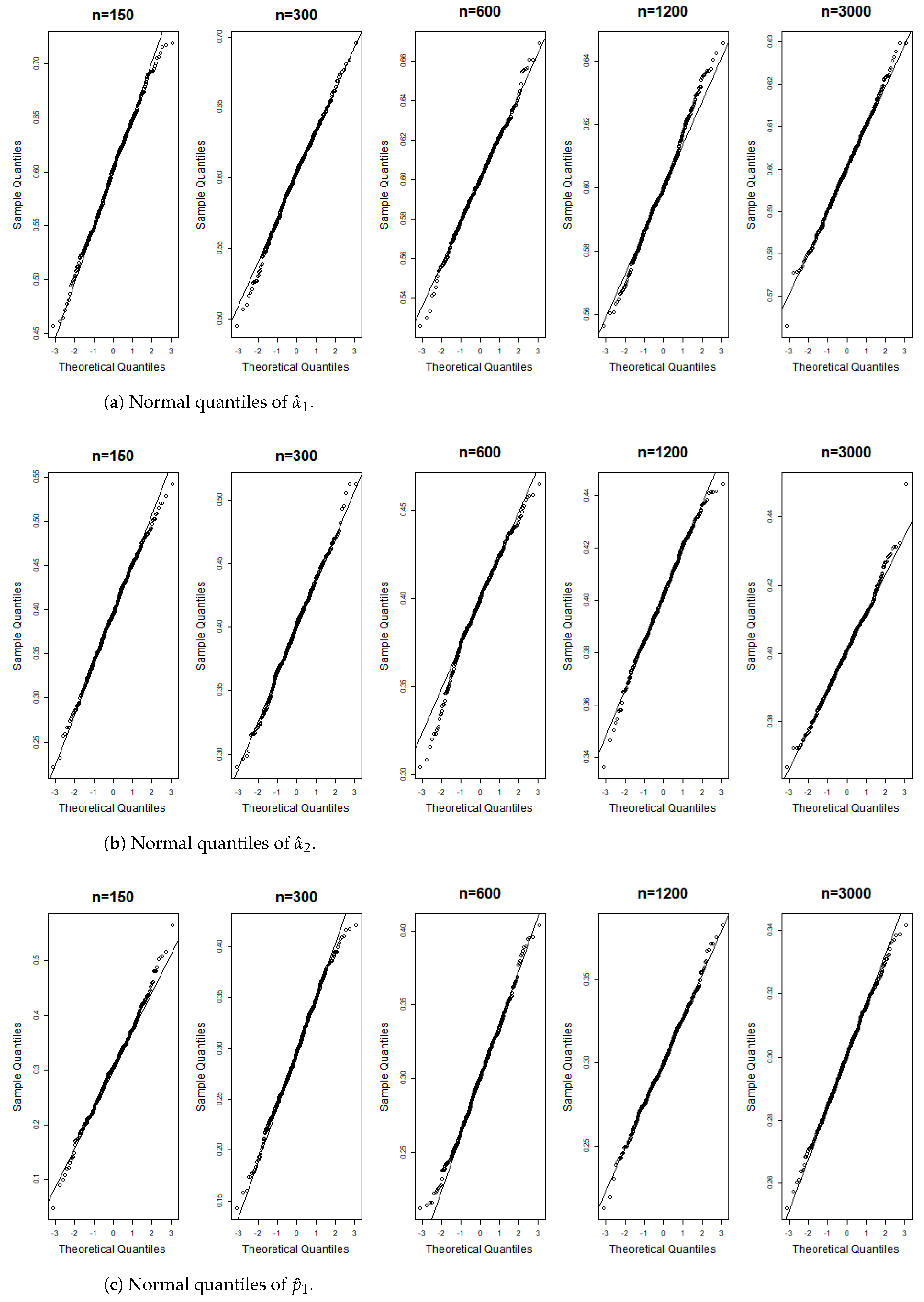
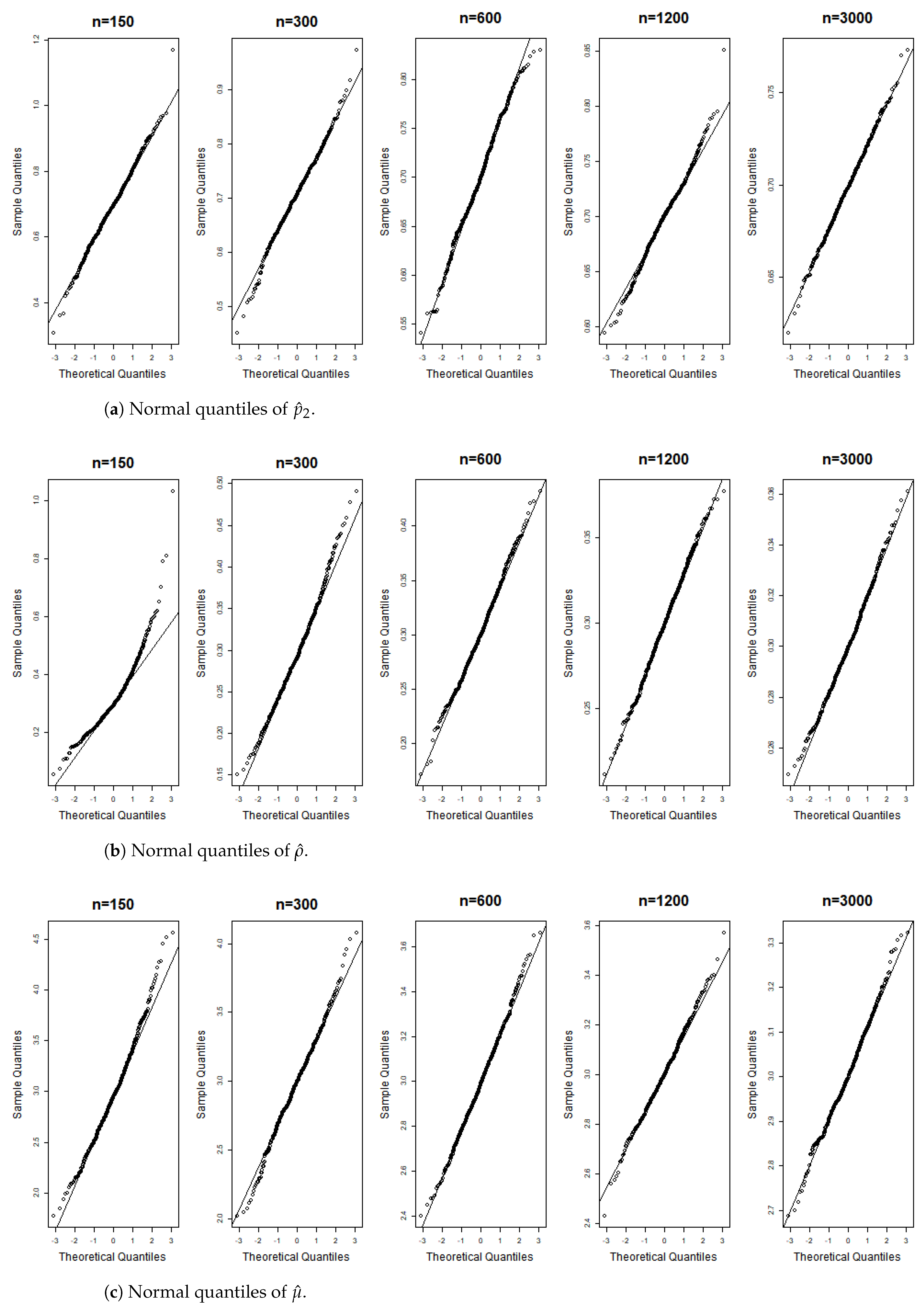
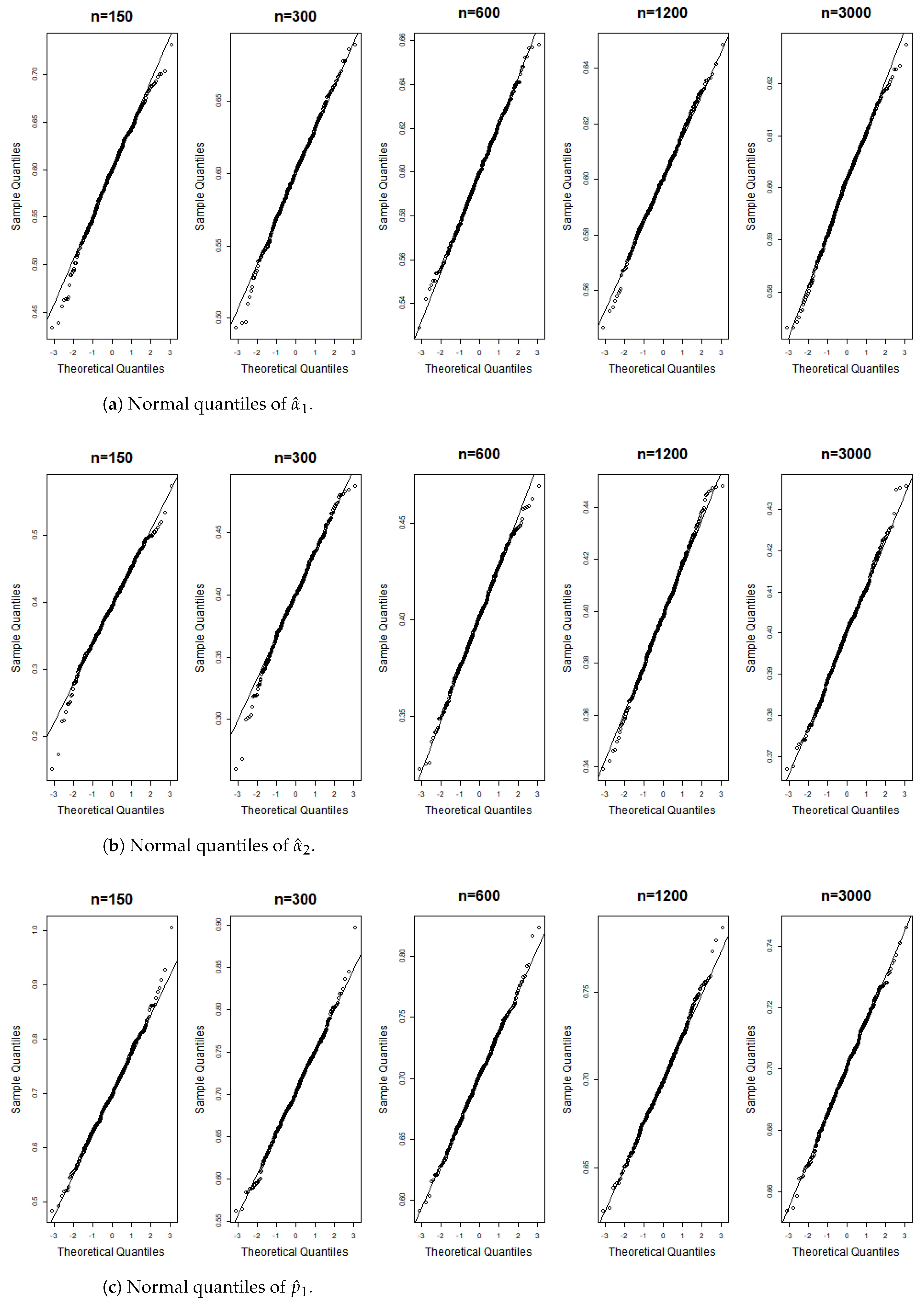
4. Estimation Procedure

In this section, we consider ${\mathit{X}}_t$ as a strictly stationary and ergodic solution of the $\rho$-BVGINAR(1) process, with ${\left\{{\mathit{X}}_t\right\}}_{t\in \mathbb{Z}}$ representing a series of observations generated from this process. We discuss the estimation of the model parameters, comprising six parameters: one for thinning the distribution ($\rho$), two for the autocorrelation coefficients (${\alpha }_1,{\alpha }_2$), two for specifying the dependence between processes $X_{1,t}$ and $X_{2,t}$ ($p_1,p_2$), and one for the marginal distributions ($\mu$). Considering the unique characteristics of these parameters, we integrate two estimation approaches: the Yule–Walker (YW) and the conditional maximum likelihood (CML) methods.

The sample mean is commonly employed for estimating model parameters in time series analysis. Since the model assumption is that the marginal distribution $\left\{X_{i,t}\right\}\stackrel{d}{=}Geom\left(\frac{\mu }{1+\mu }\right)$, then $\mu =E\left(X_{1,t}\right)=E\left(X_{2,t}\right)$. Thus, the reasonable estimate would be:

$${\widehat{\mu }}^{YW}=\frac{1}{2n}\sum _{j=1}^n(X_{1,j}+X_{2,j}).$$

Theorem 2. 

The estimator ${\widehat{\mu }}^{YW}$ is strongly consistent.

Proof. 

Proposition 1 proved that process $\left\{{\mathit{X}}_t\right\}$ is stationary and ergodic. Then, processes $\left\{X_{1,t}\right\}$ and $\left\{X_{2,t}\right\}$ are jointly stationary, which implies that $\frac{1}{2}(X_{1,t}+X_{2,t})$ is also stationary and ergodic. We have

$$\frac{1}{2n}\sum _{j=1}^n(X_{1,j}+X_{2,j})\stackrel{\mathrm{a}.\mathrm{s}.}{\to }\frac{1}{2}E(X_{1,t}+X_{2,t}).$$

Therefore, ${\widehat{\mu }}^{YW}\stackrel{\mathrm{a}.\mathrm{s}.}{\to }\mu .$ The proof of Theorem 2 is complete. □

Theorem 3. 

The estimator ${\widehat{\mu }}^{YW}$ is asymptotically normally distributed with parameters $(\mu ,t^{-1}{v}_s)$, where $v_s={\sum }_{k=-\infty }^{\infty }Cov(S_t,S_{t-k})$ and $S_t=\frac{1}{2}(X_{1,t}+X_{2,t})$.

In addition, the conditional maximum likelihood (CML) stands out as one of the most commonly employed techniques for parameter estimation. The CML estimator of parameter vector $\mathit{\theta }={({\alpha }_1,{\alpha }_2,p_1,p_2,\rho )}^{\top }$ is the value $\widehat{\mathit{\theta }}={({\widehat{\alpha }}_1,{\widehat{\alpha }}_2,{\widehat{p}}_1,{\widehat{p}}_2,\widehat{\rho })}^{\top }$ that maximizes the conditional log-likelihood function $L\left(\mathit{\theta }\right)$. Suppose that ${\mathit{X}}_1$ is fixed. The conditional log-likelihood function is given by

$$L\left(\mathit{\theta }\right)=\sum _{t=2}^{T}log\left\{P(X_{1,t}=x,X_{2,t}=y|X_{1,t-1}=u,X_{2,t-1}=v,\mathit{\theta })\right\}.$$

(13)

Under the given conditions, the conditional probability mass functions of processes $X_{1,t}$ and $X_{2,t}$ can be represented as the products of their respective conditional probabilities. These probabilities result from the convolution of the $\rho$-binomial distribution and the probability mass function of the corresponding innovation processes. Specifically,

$$\begin{array}{cc}\hfill L\left(v\right)=& \sum _{t=2}^{n}log\left[P(X_{1,t}=x|X_{1,t-1}=u,X_{2,t-1}=v)\right]+\sum _{t=2}^{n}log\left[P(X_{2,t}=y|X_{1,t-1}=u,X_{2,t-1}=v)\right]\hfill \\ \hfill =& \sum _{t=2}^{n}log\left[\left(p_1{(1-{\alpha }_1)}^u+(1-p_1){(1-{\alpha }_1)}^v\right)\right(\frac{{\mu }^x}{{(1+\mu )}^{x+1}}(1-\frac{{\alpha }_1\mu (1+\rho )}{\mu -\rho })+\frac{{\rho }^x}{{(1+\rho )}^{x+1}}\hfill \\ \hfill & \times \frac{{\alpha }_1\mu (1+\rho )}{\mu -\rho })+(p_1\sum _{k=1}^x{(1-{\alpha }_1)}^u{\left(\frac{\rho }{1+\rho }\right)}^k\sum _{i=1}^{min(k,u)}{(}_u^i){(}_{k-1}^{i-1}){\left(\frac{{\alpha }_1}{\rho (1-{\alpha }_1)}\right)}^i+(1-p_1)\hfill \\ \hfill & \times \sum _{k=1}^x{(1-{\alpha }_1)}^v{\left(\frac{\rho }{1+\rho }\right)}^k\sum _{i=1}^{min(k,v)}{(}_v^i){(}_{k-1}^{i-1}){\left(\frac{{\alpha }_1}{\rho (1-{\alpha }_1)}\right)}^i\left)\right(\frac{{\mu }^{x-k}}{{(1+\mu )}^{x+1-k}}1-\frac{{\alpha }_1\mu (1+\rho )}{\mu -\rho })\hfill \\ \hfill & +\frac{{\rho }^{x-k}}{{(1+\rho )}^{x+1-k}}\left(\frac{{\alpha }_1\mu (1+\rho )}{\mu -\rho }\right)\left)\right]+\sum _{t=2}^{n}log[\left(p_2{(1-{\alpha }_2)}^u+(1-p_2){(1-{\alpha }_2)}^v\right)\hfill \\ \hfill & \times \left(\frac{{\mu }^y}{{(1+\mu )}^{y+1}}(1-\frac{{\alpha }_2\mu (1+\rho )}{\mu -\rho })+\frac{{\rho }^y}{{(1+\rho )}^{y+1}}\frac{{\alpha }_2\mu (1+\rho )}{\mu -\rho }\right)+(p_2\sum _{k=1}^y{(1-{\alpha }_2)}^u{\left(\frac{\rho }{1+\rho }\right)}^k\hfill \\ \hfill & \times \sum _{i=1}^{min(k,u)}{(}_u^i){(}_{k-1}^{i-1}){\left(\frac{{\alpha }_2}{\rho (1-{\alpha }_2)}\right)}^i+(1-p_2)\sum _{k=1}^y{(1-{\alpha }_2)}^v{\left(\frac{\rho }{1+\rho }\right)}^k\sum _{i=1}^{min(k,v)}{(}_v^i){(}_{k-1}^{i-1})\hfill \\ \hfill & \times {\left(\frac{{\alpha }_2}{\rho (1-{\alpha }_2)}\right)}^i\left)\left(\frac{{\mu }^{y-k}}{{(1+\mu )}^{y+1-k}}(1-\frac{{\alpha }_2\mu (1+\rho )}{\mu -\rho })+\frac{{\rho }^{y-k}}{{(1+\rho )}^{y+1-k}}\left(\frac{{\alpha }_2\mu (1+\rho )}{\mu -\rho }\right)\right)\right].\hfill \end{array}$$

The likelihood function reveals that the parameters ${\alpha }_1,{\alpha }_2,\rho$, and $\mu$ often interact multiplicatively, posing significant challenges for the optimization process. To address potential issues with parameter identifiability and leverage the specific characteristics of these parameters, we have implemented a stepwise optimization strategy. Initially, we estimate $\mu$ using the Yule–Walker method. This estimate ${\widehat{\mu }}^{YW}$ is then incorporated back into the likelihood function to facilitate the optimization of the remaining parameters. This tailored approach effectively mitigates the risk of converging to local optima: a prevalent concern with non-convex objective functions.

For numerical maximization, we employ the “nlm” function from R programming software. All computational experiments were performed using R version 4.0.3 on a system equipped with an Intel Xeon Gold 6154 processor (Intel Corporation, Santa Clara, CA, USA) and 256 GB of RAM.

Next, we present the detailed simulation study design and results. We generated $\rho$-BVGINAR(1) samples with various model parameterizations and sample sizes $n=150,300,600,1200,3000$, where $n=300$ is close to the length of the crime counts that will be analyzed in Section 5. We considered the following parameter configurations:

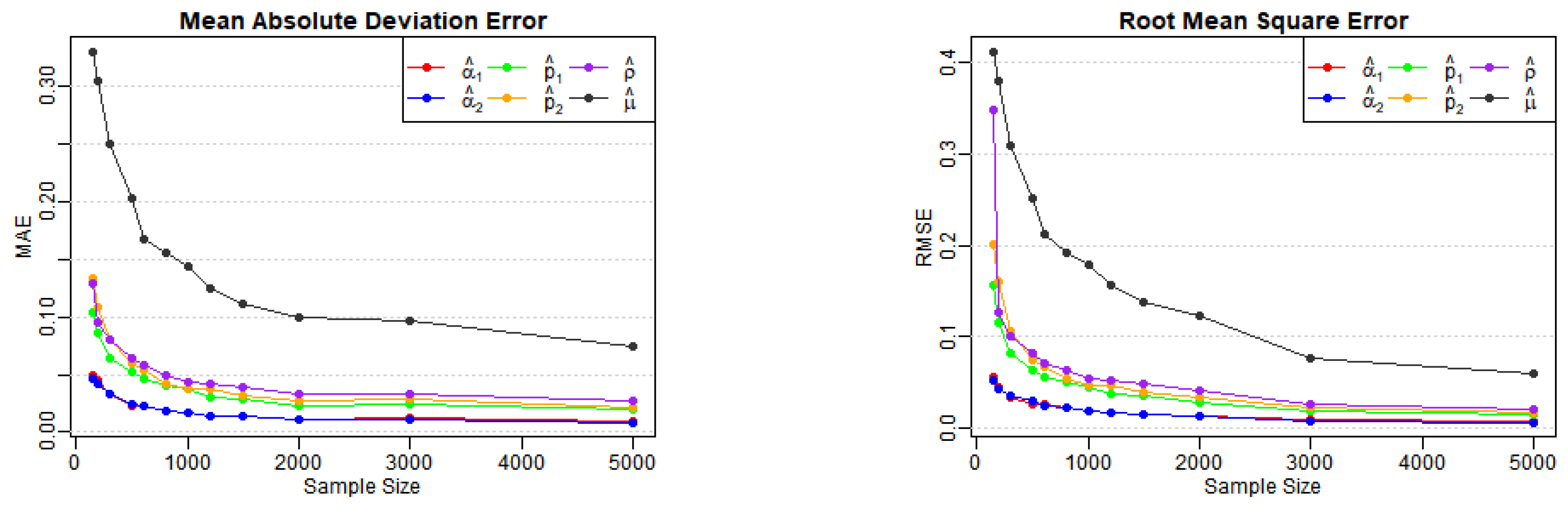
• Model (A): (${\alpha }_1,{\alpha }_2,p_1,p_2,\rho ,\mu$) = (0.3, 0.25, 0.2, 0.15, 0.1, 5);
• Model (B): (${\alpha }_1,{\alpha }_2,p_1,p_2,\rho ,\mu$) = (0.3, 0.25, 0.2, 0.15, 0.3, 5);
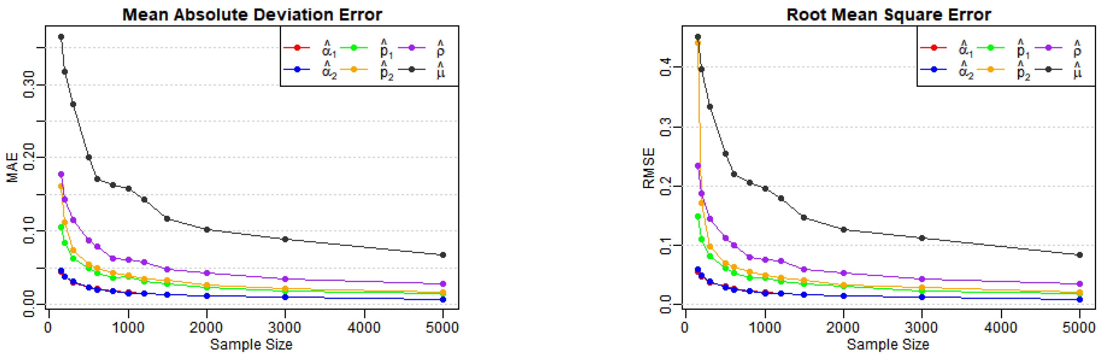
• Model (C): (${\alpha }_1,{\alpha }_2,p_1,p_2,\rho ,\mu$) = (0.4, 0.4, 0.2, 0.15, 0.25, 5);
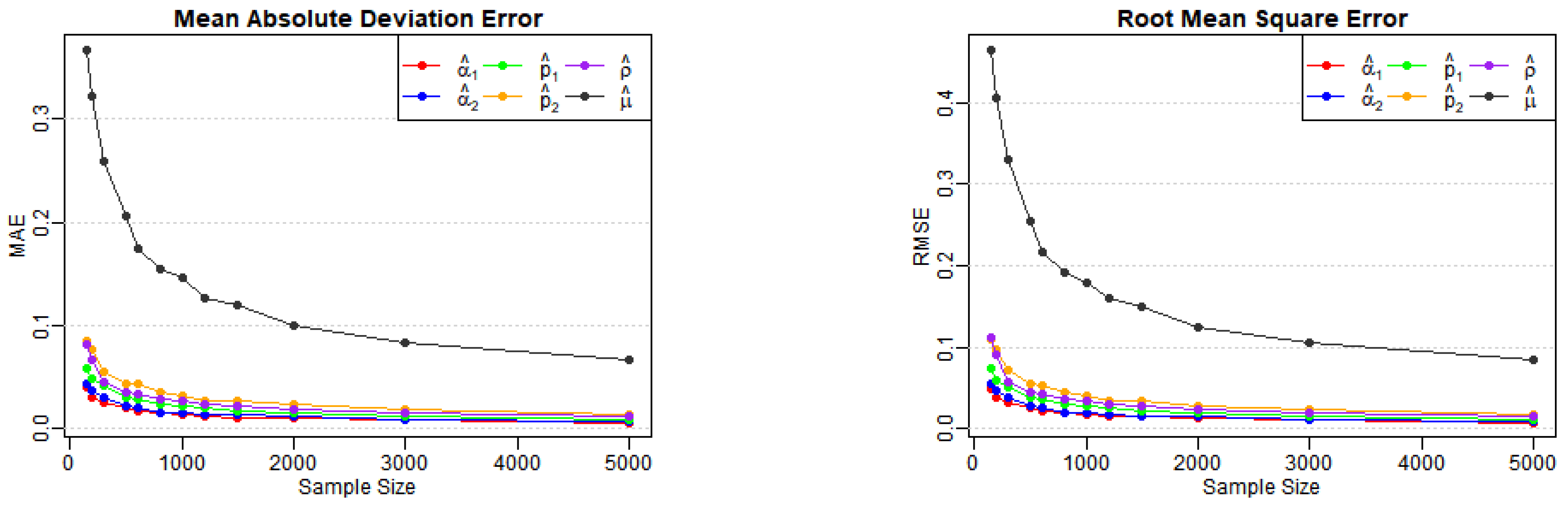
• Model (D): (${\alpha }_1,{\alpha }_2,p_1,p_2,\rho ,\mu$) = (0.6, 0.4, 0.3, 0.7, 0.3, 3);
• Model (E): (${\alpha }_1,{\alpha }_2,p_1,p_2,\rho ,\mu$) = (0.6, 0.4, 0.7, 0.3, 0.3, 3).

Recalling the properties of IBe random variables discussed in Section 2, we explored diverse parameter combinations of ${\alpha }_1$, ${\alpha }_2$, and $\rho$ in our simulation study. Models (A), (B), and (C) represent scenarios of underdispersion ($\rho <\frac{{\alpha }_1}{2-{\alpha }_1},\frac{{\alpha }_2}{2-{\alpha }_2}$), overdispersion ($\rho >\frac{{\alpha }_1}{2-{\alpha }_1},\frac{{\alpha }_2}{2-{\alpha }_2}$), and equidispersion ($\rho =\frac{{\alpha }_1}{2-{\alpha }_1},\frac{{\alpha }_2}{2-{\alpha }_2}$) of the IBe random variables $W_i({\alpha }_1,\rho )$ and $W_i({\alpha }_2,\rho )$ under $\rho$-thinning. Conversely, Models (D) and (E) are characterized by distinct dispersion patterns of $W_i({\alpha }_1,\rho )$ and $W_i({\alpha }_2,\rho )$. Specifically, Model (D) sets underdispersion of $W_i({\alpha }_1,\rho )$ and overdispersion of $W_i({\alpha }_2,\rho )$ ($\rho <\frac{{\alpha }_1}{2-{\alpha }_1}$, $\rho >\frac{{\alpha }_2}{2-{\alpha }_2}$), while Model (E) shows overdispersion of $W_i({\alpha }_1,\rho )$ and underdispersion of $W_i({\alpha }_2,\rho )$ ($\rho >\frac{{\alpha }_1}{2-{\alpha }_1}$, $\rho <\frac{{\alpha }_2}{2-{\alpha }_2}$).

To assess model performance, we employed two widely recognized criteria: mean absolute error (MAE) and root mean squared error (RMSE), based on $M=500$ replications for each model parametrization. MAE is preferred for its robustness against outliers, while RMSE provides a more detailed measure of errors and is particularly sensitive to larger deviations. The use of both MAE and RMSE allows for a comprehensive evaluation of estimation accuracy. They are defined as follows:

$$\mathrm{MAE}=\sqrt{\frac{1}{M}\sum _{m=1}^M|{\widehat{\theta }}_m-{\theta }_m|},\mathrm{RMSE}=\sqrt{\frac{1}{M}\sum _{m=1}^M{({\widehat{\theta }}_m-{\theta }_m)}^2},$$

where ${\widehat{\theta }}_m$ is the estimate of $\theta$ at the m-th replication.

In addition, to demonstrate the asymptotic normality of the estimators, we conducted a goodness-of-fit test for normality. The Anderson-Darling (AD) test, proposed by [20], is a statistical test used to assess whether data come from a specific distribution: typically, a normal distribution. Unlike other normality tests, the AD test gives more weight to the tails of the distribution, making it more powerful for detecting non-normality. Therefore, we selected the AD test to examine the asymptotic normality of the estimators by using the procedure from the R package “nortest” authored by [21].

Table 1, Table 2 and Table 3 report the estimates, biases, MAEs, and RMSEs for Models (A)–(E) across various sample sizes, as well as the AD test statistics (denoted AD in the tables) and corresponding p-values for $n=3000$. From Table 1, we observe that the biases, MAEs, and RMSEs of the estimates for Models (A) and (B) decrease as the sample size n increases, as expected. Figure 1 and Figure 2 also illustrate the notable downward trends in MAEs and RMSEs of the estimates, implying the consistency of the proposed estimators with increasing values of n. A similar conclusion can be drawn from Table 2 and Table 3, along with the corresponding visual curves in Figure 3, Figure 4 and Figure 5. Based on the above discussions, we conclude that the estimation method can produce reliable parameter estimators.

Table 1. Simulation results for Model (A) and (B) under different sample sizes.

		Model (A)						Model (B)
		${\widehat{\mathit{\alpha }}}_{\mathit{1}}$	${\widehat{\mathit{\alpha }}}_{\mathit{2}}$	${\widehat{\mathit{p}}}_{\mathit{1}}$	${\widehat{\mathit{p}}}_{\mathit{2}}$	$\widehat{\mathit{\rho }}$	$\widehat{\mathit{\mu }}$	${\widehat{\mathit{\alpha }}}_{\mathit{1}}$	${\widehat{\mathit{\alpha }}}_{\mathit{2}}$	${\widehat{\mathit{p}}}_{\mathit{1}}$	${\widehat{\mathit{p}}}_{\mathit{2}}$	$\widehat{\mathit{\rho }}$	$\widehat{\mathit{\mu }}$
Size	Metrics	0.30	0.25	0.20	0.15	0.10	5.00	0.30	0.25	0.20	0.15	0.30	5.00
150	Est.	0.2913	0.2410	0.1665	0.1028	0.1388	4.9929	0.2966	0.2413	0.1782	0.0823	0.3104	4.9649
	Bias	−0.0087	−0.0090	−0.0335	−0.0472	0.0388	−0.0071	−0.0034	−0.0087	−0.0218	−0.0677	0.0104	−0.0351
	MAE	0.0500	0.0465	0.1036	0.1341	0.1284	0.3299	0.0449	0.0465	0.1047	0.1621	0.1776	0.3656
	RMSE	0.0555	0.0527	0.1559	0.2008	0.3483	0.4113	0.0547	0.0582	0.1476	0.4420	0.2344	0.4522
300	Est.	0.2933	0.2431	0.1887	0.1351	0.1071	5.0062	0.3045	0.2521	0.1983	0.1440	0.2921	5.0100
	Bias	−0.0067	−0.0069	−0.0113	−0.0149	0.0071	0.0062	0.0045	0.0021	−0.0017	−0.0060	−0.0079	0.0100
	MAE	0.0327	0.0326	0.0638	0.0802	0.0798	0.2506	0.0298	0.0312	0.0632	0.0746	0.1149	0.2724
	RMSE	0.0344	0.0354	0.0822	0.1059	0.1004	0.3080	0.0373	0.0387	0.0821	0.0980	0.1447	0.3337
600	Est.	0.2964	0.2457	0.1985	0.1398	0.1012	4.9958	0.3009	0.2497	0.2025	0.1456	0.2975	5.0169
	Bias	−0.0036	−0.0043	−0.0015	−0.0102	0.0012	−0.0042	0.0009	−0.0003	0.0025	−0.0044	−0.0025	0.0169
	MAE	0.0234	0.0224	0.0463	0.0535	0.0579	0.1670	0.0209	0.0191	0.0420	0.0494	0.0789	0.1719
	RMSE	0.0259	0.0252	0.0568	0.0669	0.0706	0.2125	0.0259	0.0239	0.0540	0.0641	0.0990	0.2194
1200	Est.	0.2989	0.2492	0.1992	0.1449	0.1033	5.0021	0.3011	0.2495	0.1980	0.1475	0.2991	5.0012
	Bias	−0.0011	−0.0008	−0.0008	−0.0051	0.0033	0.0021	0.0011	−0.0005	−0.0020	−0.0025	−0.0009	0.0012
	MAE	0.0146	0.0143	0.0303	0.0380	0.0423	0.1252	0.0152	0.0143	0.0309	0.0353	0.0571	0.1424
	RMSE	0.0173	0.0173	0.0377	0.0478	0.0520	0.1563	0.0192	0.0178	0.0391	0.0445	0.0724	0.1784
3000	Est.	0.2998	0.2505	0.1990	0.1492	0.1001	5.0058	0.2999	0.2497	0.1992	0.1485	0.2997	4.9988
	Bias	−0.0002	0.0005	−0.0010	−0.0008	0.0001	0.0058	−0.0001	−0.0003	−0.0008	−0.0015	−0.0003	−0.0012
	MAE	0.0118	0.0111	0.0242	0.0286	0.0335	0.0964	0.0097	0.0097	0.0182	0.0220	0.0343	0.0893
	RMSE	0.0095	0.0087	0.0193	0.0228	0.0266	0.0774	0.0122	0.0120	0.0229	0.0277	0.0421	0.1130
	AD	0.4014	0.4446	0.6456	0.4647	0.2335	0.1660	0.2979	0.4877	0.3091	0.4579	0.7324	0.4977
	p-value	0.3585	0.2832	0.0916	0.2534	0.7957	0.9395	0.5872	0.2227	0.5569	0.2633	0.0559	0.2106

Table 2. Simulation results of Model (C) under different sample sizes.

Model (C)
		${\widehat{\mathit{\alpha }}}_{\mathit{1}}$	${\widehat{\mathit{\alpha }}}_{\mathit{2}}$	${\widehat{\mathit{p}}}_{\mathit{1}}$	${\widehat{\mathit{p}}}_{\mathit{2}}$	$\widehat{\mathit{\rho }}$	$\widehat{\mathit{\mu }}$
Size	Metrics	0.40	0.40	0.20	0.15	0.25	5.00
150	Est.	0.3990	0.3962	0.1860	0.1320	0.2546	5.0048
	Bias	−0.0010	−0.0038	−0.0140	−0.0180	0.0046	0.0048
	MAE	0.0383	0.0382	0.0767	0.0833	0.0985	0.4698
	RMSE	0.0469	0.0476	0.1018	0.1178	0.1234	0.5860
300	Est.	0.3997	0.4005	0.1957	0.1492	0.2485	5.0276
	Bias	−0.0003	0.0005	−0.0043	−0.0008	−0.0015	0.0276
	MAE	0.0262	0.0270	0.0528	0.0497	0.0651	0.3519
	RMSE	0.0333	0.0339	0.0675	0.0642	0.0811	0.4382
600	Est.	0.4002	0.4007	0.1956	0.1492	0.2523	5.0087
	Bias	0.0002	0.0007	−0.0044	−0.0008	0.0023	0.0087
	MAE	0.0188	0.0190	0.0346	0.0351	0.0480	0.2383
	RMSE	0.0234	0.0239	0.0437	0.0433	0.0620	0.3015
1200	Est.	0.4004	0.4001	0.1978	0.1505	0.2479	4.9909
	Bias	0.0004	0.0001	−0.0022	0.0005	−0.0021	−0.0091
	MAE	0.0132	0.0120	0.0244	0.0251	0.0333	0.1745
	RMSE	0.0166	0.0151	0.0309	0.0313	0.0415	0.2153
3000	Est.	0.4005	0.4004	0.2008	0.1493	0.2490	5.0044
	Bias	0.0005	0.0004	0.0008	−0.0007	−0.0010	0.0044
	MAE	0.0079	0.0079	0.0155	0.0150	0.0208	0.1091
	RMSE	0.0101	0.0098	0.0195	0.0186	0.0258	0.1347
	AD	0.2718	0.2061	0.4386	0.2595	0.4890	0.5042
	p-value	0.6703	0.8696	0.2928	0.7118	0.2211	0.2029

Table 3. Simulation results of Model (D) and (E) under different sample sizes.

		Model (D)						Model (E)
		${\widehat{\mathit{\alpha }}}_{\mathit{1}}$	${\widehat{\mathit{\alpha }}}_{\mathit{2}}$	${\widehat{\mathit{p}}}_{\mathit{1}}$	${\widehat{\mathit{p}}}_{\mathit{2}}$	$\widehat{\mathit{\rho }}$	$\widehat{\mathit{\mu }}$	${\widehat{\mathit{\alpha }}}_{\mathit{1}}$	${\widehat{\mathit{\alpha }}}_{\mathit{2}}$	${\widehat{\mathit{p}}}_{\mathit{1}}$	${\widehat{\mathit{p}}}_{\mathit{2}}$	$\widehat{\mathit{\rho }}$	$\widehat{\mathit{\mu }}$
Size	Metrics	0.60	0.40	0.30	0.70	0.30	3.00	0.60	0.40	0.70	0.30	0.30	3.00
150	Est.	0.5989	0.3943	0.3025	0.6947	0.3106	2.9614	0.5961	0.3931	0.6987	0.2861	0.3111	2.9720
	Bias	−0.0011	−0.0057	0.0025	−0.0053	0.0106	−0.0386	−0.0039	−0.0069	−0.0013	−0.0139	0.0111	−0.0280
	MAE	0.0397	0.0441	0.0581	0.0856	0.0815	0.3666	0.0379	0.0458	0.0588	0.0856	0.0807	0.3892
	RMSE	0.0488	0.0547	0.0746	0.1103	0.1119	0.4651	0.0479	0.0583	0.0744	0.1111	0.1179	0.4905
300	Est.	0.6013	0.3991	0.2950	0.7052	0.2949	2.9846	0.5989	0.3986	0.7014	0.2971	0.2999	2.9953
	Bias	0.0013	−0.0009	−0.0050	0.0052	−0.0051	−0.0154	−0.0011	−0.0014	0.0014	−0.0029	−0.0001	−0.0047
	MAE	0.0255	0.0302	0.0417	0.0554	0.0456	0.2589	0.0256	0.0277	0.0395	0.0582	0.0495	0.2759
	RMSE	0.0322	0.0378	0.0514	0.0713	0.0575	0.3311	0.0322	0.0357	0.0497	0.0725	0.0647	0.3487
600	Est.	0.5994	0.3975	0.2995	0.7007	0.3012	2.9896	0.5989	0.4007	0.7000	0.3007	0.2992	2.9992
	Bias	−0.0006	−0.0025	−0.0005	0.0007	0.0012	−0.0104	−0.0011	0.0007	0.0000	0.0007	−0.0008	−0.0008
	MAE	0.0173	0.0211	0.0285	0.0433	0.0344	0.1738	0.0176	0.0205	0.0289	0.0393	0.0350	0.1881
	RMSE	0.0219	0.0269	0.0355	0.0535	0.0430	0.2170	0.0219	0.0256	0.0363	0.0499	0.0439	0.2390
1200	Est.	0.6004	0.4013	0.2999	0.6981	0.2984	3.0039	0.5999	0.3979	0.6994	0.3001	0.2999	3.0026
	Bias	0.0004	0.0013	−0.0001	−0.0019	−0.0016	0.0039	−0.0001	−0.0021	−0.0006	0.0001	−0.0001	0.0026
	MAE	0.0122	0.0144	0.0208	0.0273	0.0237	0.1270	0.0126	0.0156	0.0204	0.0290	0.0243	0.1447
	RMSE	0.0156	0.0179	0.0262	0.0354	0.0296	0.1602	0.0160	0.0197	0.0257	0.0365	0.0301	0.1791
3000	Est.	0.6000	0.4005	0.2998	0.6982	0.2998	3.0030	0.6007	0.3997	0.7000	0.3002	0.2982	3.0000
	Bias	0.0000	0.0005	−0.0002	−0.0018	−0.0002	0.0030	0.0007	−0.0003	0.0000	0.0002	−0.0018	0.0000
	MAE	0.0081	0.0093	0.0126	0.0183	0.0152	0.0836	0.0079	0.0093	0.0122	0.0181	0.0145	0.0856
	RMSE	0.0102	0.0118	0.0155	0.0232	0.0192	0.1054	0.0098	0.0117	0.0153	0.0226	0.0180	0.1074
	AD	0.1186	0.3962	0.2291	0.1378	0.5815	0.7015	0.7048	0.4253	0.2718	0.2414	0.2766	0.5041
	p-value	0.9898	0.3688	0.8088	0.9763	0.1297	0.0667	0.0654	0.3150	0.6705	0.7713	0.6542	0.2031

Figure 1. Variation of MAE and RMSE for Model (A) estimates across various sample sizes.

Figure 2. Variation of MAE and RMSE for Model (B) estimates across various sample sizes.

Figure 3. Variation of MAE and RMSE for Model (C) estimates across various sample sizes.

Figure 4. Variation of MAE and RMSE for Model (D) estimates across various sample sizes.

Figure 5. Variation of MAE and RMSE for Model (E) estimates across various sample sizes.

Figure 6, Figure 7, Figure 8, Figure 9, Figure 10, Figure 11, Figure 12, Figure 13, Figure 14 and Figure 15 display the Gaussian QQ plots of the proposed estimators for Models (A)–(E) across various sample sizes. For small sample sizes, particularly when $n=150$, the data points are concentrated along a non-45-degree diagonal. However, as n increases, more data points align closely with the 45-degree line, indicating a good match between the estimator and normal distributions. Furthermore, all p-values of the AD normality test for the estimates when $n=3000$ for Models (A)–(E) are greater than the significance level of 0.05, as shown in Table 1, Table 2 and Table 3, further confirming the asymptotic normality of the estimators for large sample sizes. Based on the above facts, we conclude that the proposed estimation method is trustworthy for the models under consideration and can yield estimators with asymptotic normality.

Figure 6. Gaussian QQ plots of the estimates of ${\alpha }_1,{\alpha }_2$, and $p_1$ for Model (A) across various sample sizes.

Figure 7. Gaussian QQ plots of the estimates of $p_2,\rho$, and $\mu$ for Model (A) across various sample sizes.

Figure 8. Gaussian QQ plots of the estimates of ${\alpha }_1,{\alpha }_2$, and $p_1$ for Model (B) across various sample sizes.

Figure 9. Gaussian QQ plots of the estimates of $p_2,\rho$, and $\mu$ for Model (B) across various sample sizes.

Figure 10. Gaussian QQ plots of the estimates of ${\alpha }_1,{\alpha }_2$, and $p_1$ for Model (C) across various sample sizes.

Figure 11. Gaussian QQ plots of the estimates of $p_2,\rho$, and $\mu$ for Model (C) across various sample sizes.

Figure 12. Gaussian QQ plots of the estimates of ${\alpha }_1,{\alpha }_2$, and $p_1$ for Model (D) across various sample sizes.

Figure 13. Gaussian QQ plots of the estimates of $p_2,\rho$, and $\mu$ for Model (D) across various sample sizes.

Figure 14. Gaussian QQ plots of the estimates of ${\alpha }_1,{\alpha }_2$, and $p_1$ for Model (E) across various sample sizes.

Figure 15. Gaussian QQ plots of the estimates of $p_2,\rho$, and $\mu$ for Model (E) across various sample sizes.

5. Real Data Examples

In this section, we present two applications to demonstrate the effectiveness of our proposed $\rho$-BVGINAR(1) model in capturing overdispersion and zero inflation phenomena. We compare our model with existing bivariate INAR(1) models utilizing standard binomial and negative binomial thinning operators. Specifically, we consider the following models:

• BVNGINAR(1) model ([18]);
• BVPOINAR(1) model ([4]);
• BVMIXINAR(1) model ([22]).

Note that both the binomial and negative binomial thinning operators are special cases of the $\rho$-binomial thinning operator: the three models above are considered. For fairness, we estimate the mean parameter $\mu$ using the Yule–Walker method across all models, while employing maximum likelihood estimation for other parameters. Model performance was evaluated using the Akaike information criterion (AIC) and Bayesian information criterion (BIC).

The dataset used in this analysis was obtained from the NSW Bureau of Crime Statistics and Research (BOCSAR). It is organized by local government area (LGA), offense category (including subcategories), and month. Covering the period from January 1995 to December 2023, the dataset includes 348 monthly crime counts in New South Wales (NSW), Australia. The data can be downloaded from the following website: https://www.bocsar.nsw.gov.au/Pages/bocsar_datasets/Offence.aspx, accessed on 13 May 2024.

To illustrate the characteristics of the observations, we present descriptive statistics for each series. These statistics include the minimum (Min), maximum (Max), median, mean, variance (Var), dispersion index ($I_d$), and zero inflation index ($z_0$). The $I_d$ is defined in Equation (2). The $z_0$ index, introduced by [23], is employed to assess the excess occurrence of zeros in count data and is formulated as:

$$z_0=1+\frac{ln\left(p_0\right)}{\lambda },$$

where $p_0$ denotes the proportion of zeros, and $\lambda$ represents the mean. A $z_0$ value greater than 0 indicates zero inflation, while a value less than 0 suggests zero deflation.

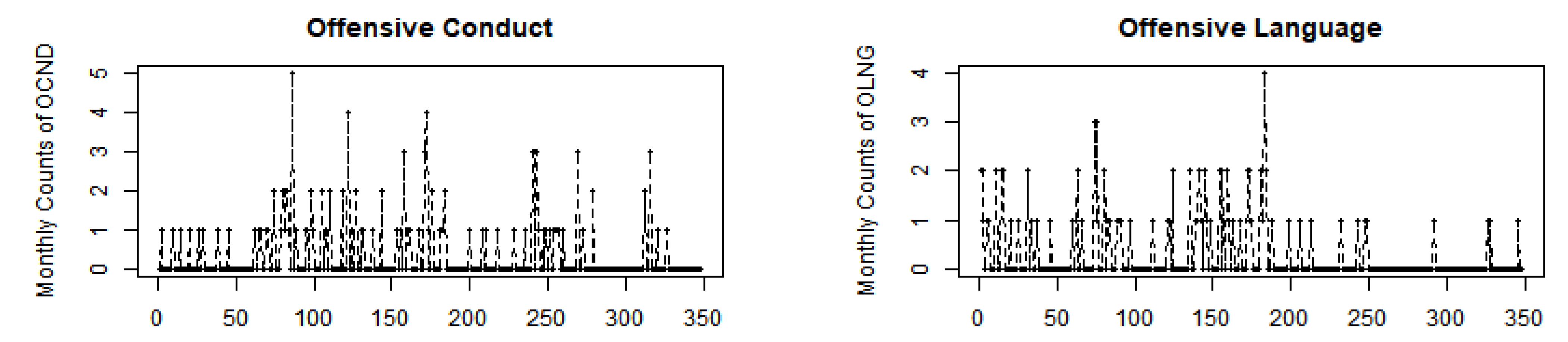
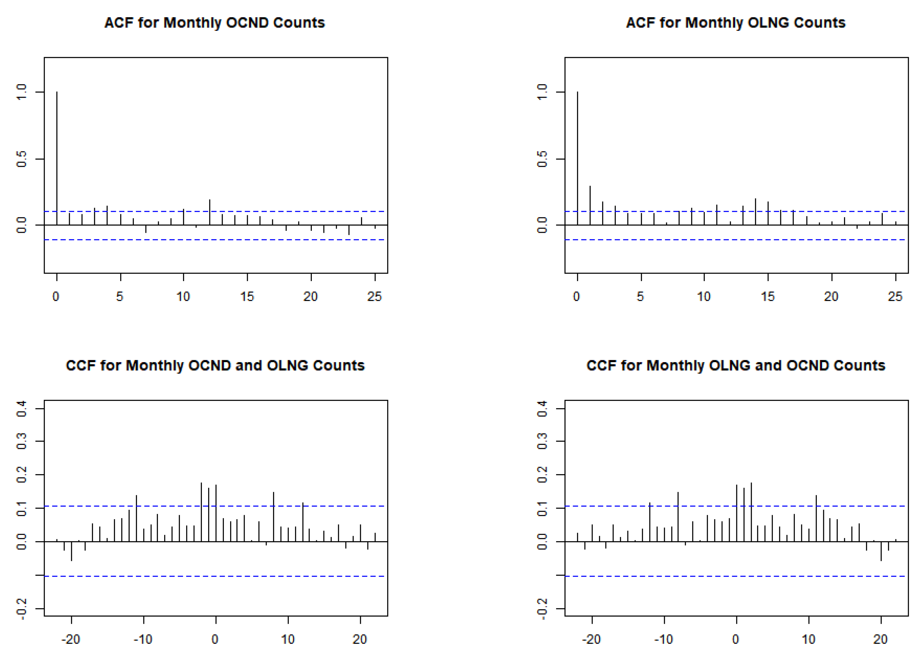
5.1. Crime Data: Disorderly Conduct Counts in Carrathool

In the first application, we analyze disorderly conduct counts in Carrathool, including three subcategories: “offensive conduct” (OCND), “offensive language” (OLNG), and “criminal intent”. Evidently, OCND and OLNG often co-occur due to similar contexts, likely indicating a significant degree of mutual association between their counts. Therefore, we applied the $\rho$-BVGINAR(1) model to fit the counts of OCND and OLNG.

The time series, autocorrelation function (ACF), and cross-correlation function (CCF) plots for the OCND and OLNG series are depicted in Figure 16 and Figure 17. The ACF plots show autocorrelation in both series, while the values in the CCF plot surpass the confidence interval, suggesting non-independence between the two series. Table 4 presents descriptive statistics for both series. The empirical mean values for OCND and OLNG are relatively close, at 0.3448 and 0.2960, respectively. Both sequences exhibit dispersion indices $I_d$ of $1.6098$ and $1.3487$, slightly exceeding 1, indicating marginal overdispersion. Moreover, the $z_0$ values for both series exceed 0, indicating zero inflation characteristics in the data. Further insight is provided by their histograms in Figure 18, which highlight a notable proportion of zeros in each series.

Figure 16. Sample paths of OCND and OLNG series.

Figure 17. The autocorrelation function (ACF) and cross-correlation (CCF) plots of OCND and OLNG series.

Table 4. Descriptive statistics of OCND and OLNG series.

Crime	Min	Max	Median	Mean	Var	${\mathit{I}}_{\mathit{d}}$	${\mathit{z}}_0$
Offensive Conduct (OCND)	0	5	0	0.3448	0.5551	1.6098	0.6616
Offensive Language (OLNG)	0	4	0	0.2960	0.3992	1.3487	0.6438

Figure 18. Histograms of OCND and OLNG counts.

The fitted results of the proposed $\rho$-BVGINAR(1), BVNGINAR(1), BVPOINAR(1), and BVMIXINAR(1) models are summarized in Table 5. Despite incorporating a mixture of binomial and negative binomial thinning, the BVMIXINAR(1) model exhibits the poorest performance, evidenced by its minimum log-likelihood value ($-526.14$), maximum AIC (1062.29) and BIC (1081.55) values. The BVNGINAR(1) and BVPOINAR(1) models perform comparably based on their log-likelihood values, appearing only suboptimal compared to the $\rho$-BVGINAR(1) model. However, the $\rho$-BVGINAR(1) model achieves the lowest AIC (991.27) and BIC (1008.53) values, indicating superior data fitting.

Table 5. Fitting results of the monthly OCND and OLNG counts across different models.

Estimate	$\mathit{\rho }$-BVGINAR(1)	BVNGINAR(1)	BVPOINAR(1)	BVMIXINAR(1)
${\widehat{\alpha }}_1$	0.1278	0.2364	0.0769	0.3306
${\widehat{\alpha }}_2$	0.3435	0.1695	0.5340	0.2339
${\widehat{p}}_1$	0.5724	0.2289	0.6902	0.3071
${\widehat{p}}_2$	0.6263	0.2572	0.2078	0.0961
$\widehat{\rho }$	0.0777	–	–	–
$\widehat{\mu }$	0.3448	0.3448	0.3448	0.3448
LogLik	−489.64	−492.15	−492.25	−526.14
AIC	991.27	994.31	994.51	1062.29
BIC	1008.53	1013.57	1013.77	1081.55

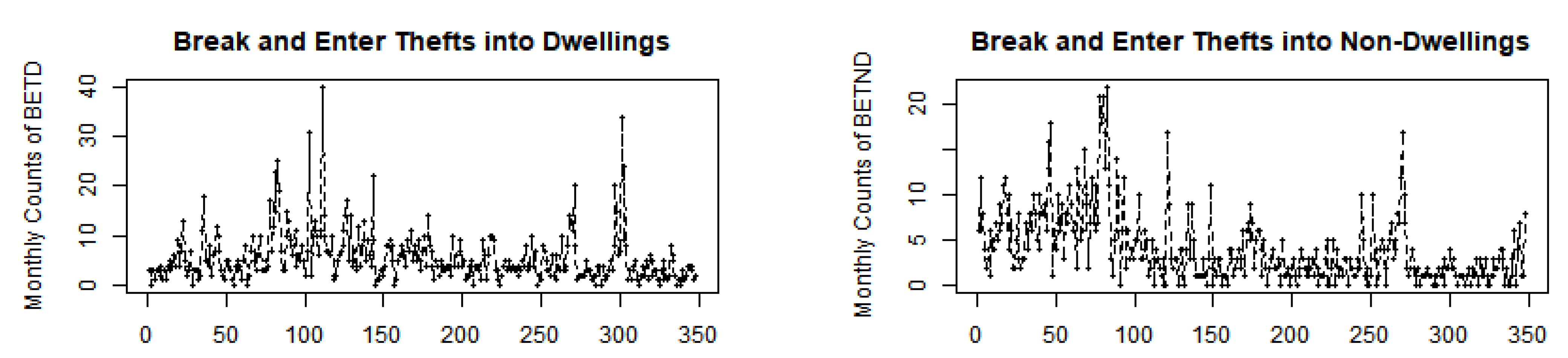
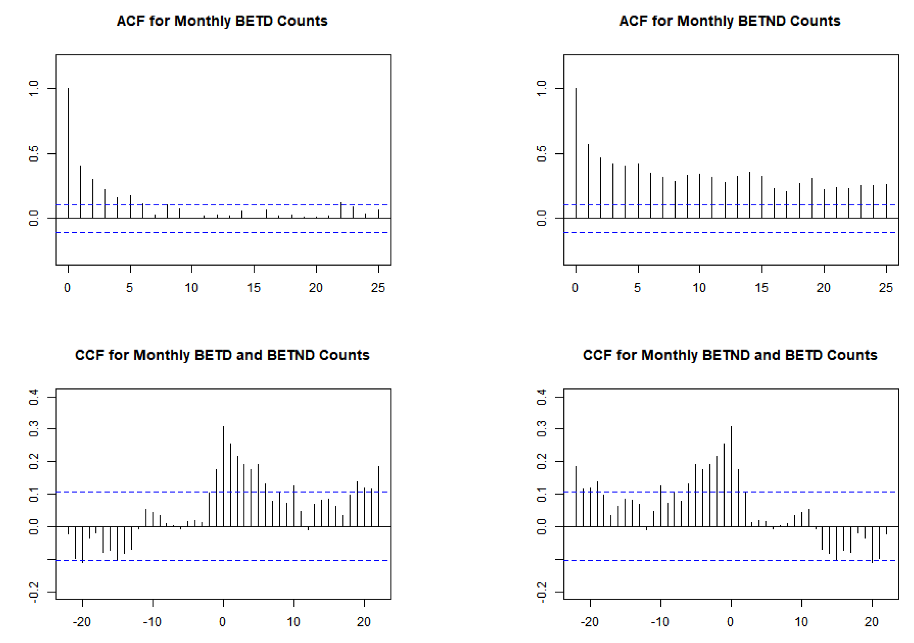
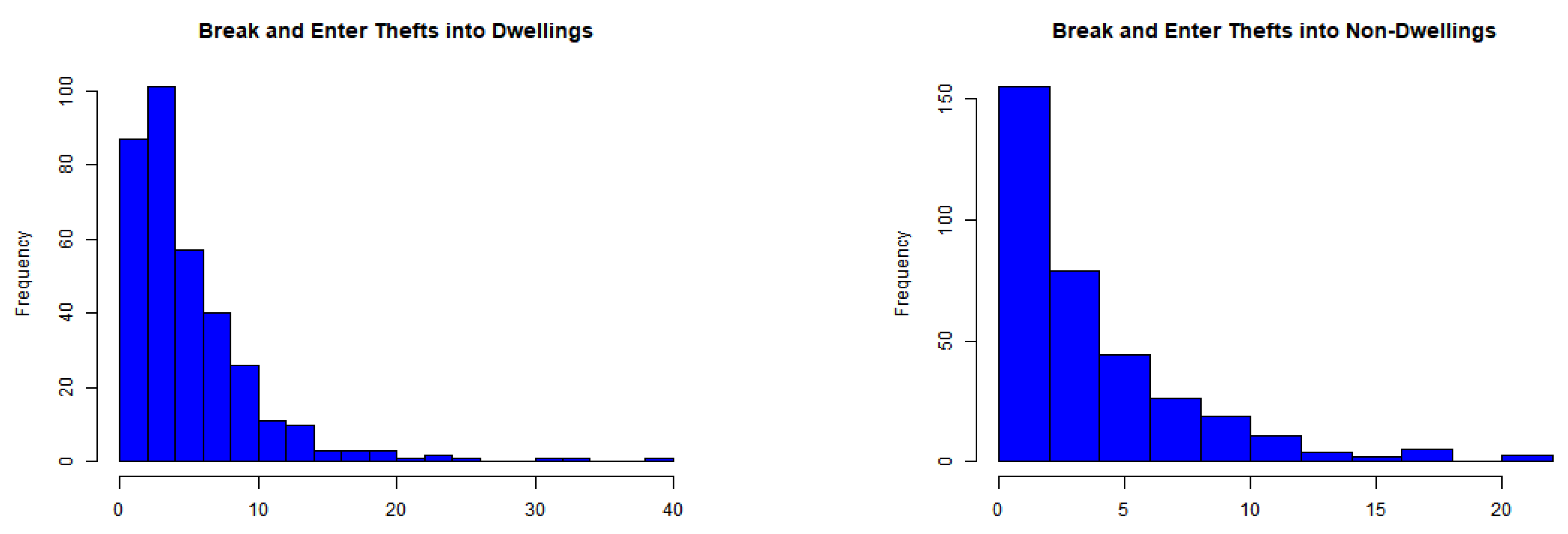
5.2. Crime Data: Theft Counts in Narrandera

As suggested by a referee, to demonstrate the flexibility and applicability of our model, we selected a real-world example with higher levels of overdispersion for analysis. We focused on the theft counts in Narrandera, encompassing five subcategories: “break and enter dwelling”, “break and enter non-dwelling”, “receiving or handling stolen goods”, “motor vehicle theft”, and “steal from motor vehicle”. Notably, “break and enter dwelling” and “break and enter non-dwelling” exhibit a correlation due to their similar modus operandi and motivations, likely originating from the actions of the same group of offenders. Therefore, we chose to examine the counts of “break and enter thefts into dwelling” (BETD) and “break and enter theft into non-dwelling” (BETND) for further investigation.

Figure 19 and Figure 20 display the time series, ACF, and CCF plots, revealing significant autocorrelation within each series and cross-correlation between the BETD and BETND series. Table 6 presents the dispersion indices $I_d$ values of $4.6408$ and $3.9099$, markedly exceeding 1, indicating a higher degree of overdispersion compared to the $I_d$ values of $1.6098$ and $1.3487$ observed in the OCND and OLNG counts. Moreover, the $z_0$ values for both series indicate notable zero inflation, with values of $0.7587$ and $0.7681$, respectively. Their histograms are depicted in Figure 21.

Figure 19. Sample paths of BETD and BETND series.

Figure 20. The autocorrelation function (ACF) and cross-correlation (CCF) plots of BETD and BETND series.

Table 6. Descriptive statistics of BETD and BETND series.

Crime	Min	Max	Median	Mean	Var	${\mathit{I}}_{\mathit{d}}$	${\mathit{z}}_0$
Break and Enter Thefts into Dwellings (BETD)	0	40	4	5.5431	25.7244	4.6408	0.7587
Break and Enter Thefts into Non-Dwellings (BETND)	0	22	3	4.0517	15.8417	3.9099	0.7681

Figure 21. Histograms of BETD and BETND counts.

Table 7 presents the fitted results. We observe that the BVMIXINAR(1) model exhibits the highest AIC and BIC values, indicating that the model fails to capture the overdispersion and zero inflation characteristic of the dataset. We also notice that the BIC value of the fitted BVPOINAR(1) models is also large, indicating that the model is unsuitable to fit this dataset. While the BVNGINAR(1) model yields satisfactory results, the $\rho$-BVGINAR(1) model outperforms it in terms of AIC and BIC values, indicating its greater suitability for fitting the BETD and BETND counts.

Table 7. Fitting results of the monthly BETD and BETND counts across different models.

Estimate	$\mathit{\rho }$-BVGINAR(1)	BVNGINAR(1)	BVPOINAR(1)	BVMIXINAR(1)
${\widehat{\alpha }}_1$	0.2434	0.7028	0.3483	0.6987
${\widehat{\alpha }}_2$	0.2686	0.6855	0.5614	0.7911
${\widehat{p}}_1$	0.7451	0.3911	0.9741	0.4548
${\widehat{p}}_2$	0.2428	0.2431	0.3223	0.4693
$\widehat{\rho }$	1.5649	–	–	–
$\widehat{\mu }$	5.5431	5.5431	5.5431	5.5431
LogLik	−1742.96	−1761.20	−1987.37	−2216.58
AIC	3497.91	3532.40	3984.75	4443.16
BIC	3515.17	3551.66	4004.01	4462.42

In conclusion, the $\rho$-BVGINAR(1) model outperforms the other three models and more effectively captures the overdispersion and zero inflation features in count time series data. It demonstrates superiority in model fitting by striking a balance between flexibility and complexity.

6. Conclusions

This paper introduces a more flexible $\rho$-BVGINAR(1) model tailored to analyzing bivariate integer-valued time series data with overdispersion characteristic. It extends the $\rho$-GINAR(1) model [12] to the two-dimensional case. Meanwhile, it is also a generalization of the BVGNAR(1) model or the BVNGINAR(1) model [18], offering enhanced capability for handling excess zeros and overdispersed data. Furthermore, the paper derives the innovation structure of the proposed model, discusses its essential properties, and describes the methodologies for YW and CML estimation. A comprehensive simulation study is conducted to evaluate the finite sample performances of the estimators and their asymptotic properties under various parameter combinations. Two real applications showcase the effectiveness of the proposed model relative to existing ones, demonstrating its utility in practical settings.

Moving forward, there are several promising avenues for future research in the field of bivariate INAR-type models. One promising direction involves exploring the application of the zero-modified geometric distribution as the marginal distribution. This distribution offers the capability to effectively model features such as zero inflation, zero deflation, overdispersion, and underdispersion, as discussed in detail in [24]. In addition, there is potential for further investigation into the modification of various marginal parameters and thinning parameters. Previous works, such as those by [7,19], have demonstrated the effectiveness of such modifications for analyzing bivariate time series data. These approaches hold promise for enhancing the flexibility and applicability of bivariate models and warrant thorough exploration in future research projects.

References

- Brannas, K.; Nordstrom, J. A Bivariate Integer Valued Allocation Model for Guest Nights in Hotels and Cottages. Umea Economic Studies Working Paper No. 547. 2001. Available online: https://ssrn.com/abstract=255292 (accessed on 20 May 2024). [CrossRef]
- Quoreshi, A.S. Bivariate time series modeling of financial count data. Commun. Stat. Theory Methods 2006, 35, 1343–1358. [Google Scholar] [CrossRef]
- Pedeli, X.; Karlis, D. A bivariate INAR (1) process with application. Stat. Model. 2011, 11, 325–349. [Google Scholar] [CrossRef]
- Nastić, A.S.; Ristić, M.M.; Popović, P.M. Estimation in a bivariate integer-valued autoregressive process. Commun. Stat. Theory Methods 2016, 45, 5660–5678. [Google Scholar] [CrossRef]
- Khan, N.M.; Oncel Cekim, H.; Ozel, G. The family of the bivariate integer-valued autoregressive process (BINAR (1)) with Poisson–Lindley (PL) innovations. J. Stat. Comput. Simul. 2020, 90, 624–637. [Google Scholar] [CrossRef]
- Chen, H.; Zhu, F.; Liu, X. A new bivariate INAR (1) model with time-dependent innovation vectors. Stats 2022, 5, 819–840. [Google Scholar] [CrossRef]
- Popović, P.M.; Ristić, M.M.; Nastić, A.S. A geometric bivariate time series with different marginal parameters. Stat. Pap. 2016, 57, 731–753. [Google Scholar] [CrossRef]
- Yu, M.; Wang, D.; Yang, K.; Liu, Y. Bivariate first-order random coefficient integer-valued autoregressive processes. J. Stat. Plan. Inference 2020, 204, 153–176. [Google Scholar] [CrossRef]
- Su, B.; Zhu, F. Comparison of BINAR (1) models with bivariate negative binomial innovations and explanatory variables. J. Stat. Comput. Simul. 2021, 91, 1616–1634. [Google Scholar] [CrossRef]
- Steutel, F.W.; van Harn, K. Discrete analogues of self-decomposability and stability. Ann. Probab. 1979, 7, 893–899. [Google Scholar] [CrossRef]
- Al-Osh, M.A.; Aly, E.-E.A. First order autoregressive time series with negative binomial and geometric marginals. Commun. Stat. Theory Methods 1992, 21, 2483–2492. [Google Scholar] [CrossRef]
- Borges, P.; Molinares, F.F.; Bourguignon, M. A geometric time series model with inflated-parameter Bernoulli counting series. Stat. Probab. Lett. 2016, 119, 264–272. [Google Scholar] [CrossRef]
- Kachour, M.; Truquet, L. A p-order signed integer-valued autoregressive (SINAR (p)) model. J. Time Ser. Anal. 2011, 32, 223–236. [Google Scholar] [CrossRef]
- Bulla, J.; Chesneau, C.; Kachour, M. A bivariate first-order signed integer-valued autoregressive process. Commun. Stat. Theory Methods 2017, 46, 6590–6604. [Google Scholar] [CrossRef]
- Zhang, Q.; Wang, D.; Fan, X. A negative binomial thinning-based bivariate INAR (1) process. Stat. Neerl. 2020, 74, 517–537. [Google Scholar] [CrossRef]
- Ristić, M.M.; Bakouch, H.S.; Nastić, A.S. A new geometric first-order integer-valued autoregressive (NGINAR (1)) process. J. Stat. Plan. Inference 2009, 139, 2218–2226. [Google Scholar] [CrossRef]
- Kolev, N.; Minkova, L.; Neytchev, P. Inflated-parameter family of generalized power series distributions and their application in analysis of overdispersed insurance data. ARCH Res. Clear. House 2000, 2, 295–320. [Google Scholar]
- Ristić, M.M.; Nastić, A.S.; Jayakumar, K.; Bakouch, H.S. A bivariate INAR (1) time series model with geometric marginals. Appl. Math. Lett. 2012, 25, 481–485. [Google Scholar] [CrossRef]
- Popović, P.M. A bivariate INAR (1) model with different thinning parameters. Stat. Pap. 2016, 57, 517–538. [Google Scholar] [CrossRef]
- Anderson, T.W.; Darling, D.A. A test of goodness of fit. J. Am. Stat. Assoc. 1954, 49, 765–769. [Google Scholar] [CrossRef]
- Gross, L. Tests for Normality, R Package Version 1.0-2. 2013. Available online: http://CRAN.R-project.org/package=nortest (accessed on 20 May 2024).
- Popović, P.M.; Nastić, A.S.; Ristić, M.M. Residual analysis with bivariate INAR (1) models. REVSTAT-Stat. J. 2018, 16, 349–363. [Google Scholar]
- Weiss, C.H.; Homburg, A.; Puig, P. Testing for zero inflation and overdispersion in inar (1) models. Stat. Pap. 2019, 60, 823–848. [Google Scholar] [CrossRef]
- Kang, Y.; Zhu, F.; Wang, D.; Wang, S. A zero-modified geometric INAR (1) model for analyzing count time series with multiple features. Can. J. Stat. 2023. [Google Scholar] [CrossRef]
- Brockwell, P.J.; Davis, R.A. Introduction to Time Series and Forecasting; Springer: Berlin/Heidelberg, Germany, 2002. [Google Scholar]
- Brockwell, P.J.; Davis, R.A. Time Series: Theory and Methods; Springer Science & Business Media: Berlin, Germany, 1991. [Google Scholar]
Disclaimer/Publisher’s Note: The statements, opinions and data contained in all publications are solely those of the individual author(s) and contributor(s) and not of MDPI and/or the editor(s). MDPI and/or the editor(s) disclaim responsibility for any injury to people or property resulting from any ideas, methods, instructions or products referred to in the content. |
© 2024 by the authors. Licensee MDPI, Basel, Switzerland. This article is an open access article distributed under the terms and conditions of the Creative Commons Attribution (CC BY) license (https://creativecommons.org/licenses/by/4.0/).