A C⁰ Nonconforming Virtual Element Method for the Kirchhoff Plate Obstacle Problem

Abstract

This paper investigates a novel $C^0$ nonconforming virtual element method (VEM) for solving the Kirchhoff plate obstacle problem, which is described by a fourth-order variational inequality (VI) of the first kind. In our study, we distinguish our approach by introducing new internal degrees of freedom to the traditional lowest-order $C^0$ nonconforming VEM, which originally lacked such degrees. This addition not only facilitates error estimation but also enhances its intuitiveness. Importantly, our novel $C^0$ nonconforming VEM naturally satisfies the constraints of the obstacle problem. We then establish an a priori error estimate for our novel $C^0$ nonconforming VEM, with the result indicating that the lowest order of our method achieves optimal convergence. Finally, we present a numerical example to validate the theoretical result.

1. Introduction

The Kirchhoff plate model is employed to characterize the bending behavior of thin plates. It is based on thin plate theory and is suitable for structures with relatively small thicknesses [1,2,3]. The model assumes that the thin plate remains planar during bending, disregarding thickness variations and shear deformations, and solely focusing on the bending and stretching behaviors of the plate [4]. It is widely utilized in engineering fields such as aerospace, civil engineering, and automotive engineering. Mathematically, the Kirchhoff plate problem is typically formulated as a fourth-order partial differential equation (PDE) that describes the deflection of the plate [5]. The Kirchhoff plate obstacle problem is a mathematical model utilized for investigating the behavior of thin plates in the presence of obstacles or constraints, with significant implications in various engineering and scientific fields such as structural mechanics [6] and material science.

The Kirchhoff plate obstacle problem addressed in this paper can be formulated as a typical variational inequality (VI) of the first kind [7,8]. A VI is a mathematical concept utilized to describe specific types of constrained optimization problems arising in situations where the goal is to minimize a certain functional while adhering to constraints defined by inequalities. VIs arise in various domains of mathematics and physics, such as the investigation of PDEs, optimization, and game theory [9,10,11,12]. They offer a robust framework for modeling and analyzing problems with constraints and have been extensively researched in the field of nonlinear functional analysis. In general, there is no exact solution to VIs, so it is crucial to develop effective numerical methods for solving them. Particularly, for the plate obstacle problem, which arises in various engineering and physical applications, understanding the numerical solution of these problems helps in practical engineering designs and simulations. Furthermore, developing efficient algorithms for solving the plate obstacle problem can lead to improvements in computational efficiency and accuracy. Investigating different numerical methods and their performance can help in designing better algorithms for similar types of problems [13,14,15]. Therefore, investigating the numerical solution of the plate obstacle problem is essential for advancing both the theoretical understanding of numerical methods for PDEs and their practical applications in various fields.

The virtual element method (VEM) is a numerical technique utilized for solving PDEs, initially proposed in [16]. A key characteristic of the VEM is its capability to handle general polygonal (or polyhedral) meshes and hanging nodes, which are commonly encountered in practical engineering applications but pose challenges for traditional finite element methods (FEMs) [17,18,19]. The VEM formulation allows for the utilization of different polynomial degrees or even non-polynomial functions for approximating the solution and its derivatives within an element, providing flexibility in balancing accuracy and computational cost.

Additionally, the VEM allows for the incorporation of various types of boundary conditions and material properties, making it suitable for a wide range of problems, such as linear elasticity [20,21,22], Stokes or Navier–Stokes equations [23,24,25], Cahn–Hilliard equations [26], and so on. It also has the potential to achieve high accuracy while maintaining a low computational cost, especially for problems with highly heterogeneous materials or discontinuous solutions. Overall, the VEM is a promising approach for solving PDEs, offering a flexible and efficient numerical technique that can handle a wide range of practical engineering problems. In the context of plate problems, Brezzi and Marini introduced the conforming VEM in [27]. To relax continuity requirements, Zhao et al. developed the $C^0$ nonconforming VEM for the plate problem in [28]. Subsequently, a Morley-type VEM with fewer degrees of freedom was also formulated for handling fourth-order problems [29,30].

In recent years, VEMs have been successfully used for solving variational inequalities [31,32,33,34,35,36,37]. Particularly, for the study of VIs in the plate problem, Wang and Zhao studied conforming and nonconforming VEMs for plate friction contact problems [38]. Compared to the conforming VEM, the nonconforming VEM relaxes the continuity requirements and reduces the degrees of freedom. The $C^0$ and fully nonconforming VEMs for the first kind of VI problems were studied in [39]. As a continuation of the aforementioned method, this study investigates the application of a $C^0$ nonconforming VEM to solve the Kirchhoff plate obstacle problem, which is expressed by a fourth-order VI of the first kind. For the conventional lowest-order $C^0$ nonconforming VEM, which initially lacked internal degrees of freedom, our novel approach involves introducing new internal degrees of freedom. This addition not only simplifies error estimation but also improves its intuitiveness. Crucially, our novel $C^0$ nonconforming VEM naturally satisfies the constraints of the obstacle problem. Subsequently, we establish an a priori error estimate for our novel $C^0$ nonconforming VEM. The outcome of this error estimate reveals that the lowest order of our method achieves optimal convergence. Finally, we present a numerical example to verify the results of the theoretical analysis.

The remainder of this paper is structured as follows. Section 2 outlines the plate obstacle problem and its variational formulation. Section 3 focuses on $C^0$ nonconforming VEMs for solving the target problem. In Section 4, we provide a priori error analysis, illustrating that the lowest-order VEM achieves optimal convergence order. In Section 5 presents a numerical example to verify the results of the theoretical analysis. Finally, in Section 6, we provide a summary of this paper.

2. Plate Obstacle Model

In this section, we initially present the plate obstacle model and its variational form. Subsequently, we provide detailed pointwise relations of the model.

2.1. Model Problem and Its Variational Inequality

Consider an open, bounded two-dimensional domain $\mathcal{D}$, and let $\alpha$ be a positive integer. We utilize the notations ${\parallel ·\parallel }_{\alpha ,\mathcal{D}}$ and ${|·|}_{\alpha ,\mathcal{D}}$ to represent the norm and seminorm, respectively, of the Sobolev space $H^{\alpha }\left(\mathcal{D}\right)$. When $\alpha =0$, $H^{\alpha }\left(\mathcal{D}\right)$ reduces to the standard Lebesgue space $L^2\left(\mathcal{D}\right)$ with norm ${|·|}_{\mathcal{D}}$ and the associated $L^2$ inner product ${(·,·)}_{\mathcal{D}}$. For the sake of brevity, we omit the subscript in cases where $\mathcal{D}=\Omega$. For any nonnegative integer k, ${\mathbb{P}}_k\left(\mathcal{D}\right)$ represents the space of polynomial functions with degree at most k. We denote the unit outward normal to the boundary of $\mathcal{D}$ as $\mathit{n}$ and the unit tangential vector as $\mathit{t}$. If $v\in H^1\left(\mathcal{D}\right)$, ${\partial }_{\mathit{n}}v$ and ${\partial }_{\mathit{t}}v$ denote the normal and tangential derivatives on the boundary, respectively.

Our focus is on the plate obstacle problem, which is expressed as a first-kind fourth-order elliptic variational inequality [40,41]. Given a downward force f in the center of an elastic thin plate with a fixed and non-rotatable boundary, there exists an obstacle $\psi$ beneath the plate. When the force f causes deformation of the thin plate, the bounded region $\Omega$ can be divided into two parts: the contact area ${\Omega }^0$ and the non-contact area ${\Omega }^{+}$, as shown in Figure 1. This equilibrium problem, involving the upper plate covering the obstacle $\psi$, can be described by a variational inequality in Problem P.

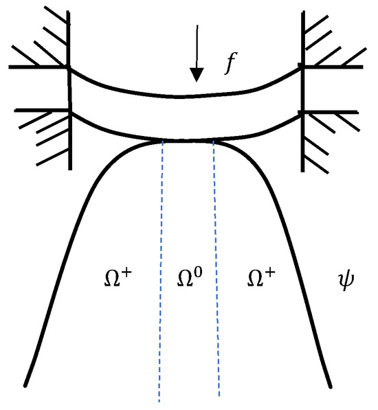
Figure 1. The obstacle problem P.

In the context of a thin plate occupying the space $\Omega \times (-d/2,d/2)$, where $\Omega \subset {\mathbb{R}}^2$ is a bounded polygonal domain and $d>0$ represents the small thickness of the plate, the boundary of $\Omega$ is denoted by $\Gamma$. Assume the material to be isotropic and linearly elastic, characterized by a positive Young’s modulus E and a positive Poisson’s ratio with $\nu <0.5$. Within this setting, let $D_{0}f$ denote the normal force density acting on the plate, and let $D_0$ represent the bending rigidity. Generally, the bending rigidity depends on the material properties of the plate and its thickness. For a thin plate, the bending rigidity can be expressed as

$$D_0=\frac{E{d}^3}{12(1-{\nu }^2)},$$

Let us consider the following elliptic variational inequality for the Kirchhoff plate obstacle problem.

Target Problem $\mathcal{T}$. For a given right-hand side $l\in L^2(\Omega )$ and obstacle $\xi \in H^2(\Omega )$ with the constraint $\xi \le 0$ on $\Gamma$, we seek to find $u\in \mathcal{S}$ that satisfies the following equation:

$$\mathcal{A}(u,v-u)\ge (l,v-u)\forall v\in \mathcal{S},$$

(1)

where

$$\mathcal{S}=\{v\in H_0^2(\Omega );v\ge \xi \mathrm{in}\Omega \}.$$

Here, the bilinear form is

$$\begin{array}{cc}\hfill \mathcal{A}(u,v)& ={\int }_{\Omega }\left[\Delta u\Delta v+(1-\nu )(2{\partial }_{12}u{\partial }_{12}v-{\partial }_{11}u{\partial }_{22}v-{\partial }_{22}u{\partial }_{11}v)\right]dx.\hfill \end{array}$$

(2)

The bilinear form $\mathcal{A}(·,·)$ in Target Problem $\mathcal{T}$ is characterized by both boundedness and coercivity, meaning that there exist constants ${\lambda }_1$ and ${\lambda }_2$ such that

$$\begin{array}{cc}& \mathcal{A}(u,v)\le {\lambda }_1{\left|u\right|}_2{\left|v\right|}_2\forall u,v\in H^2(\Omega ),\end{array}$$

(3)

$$\begin{array}{cc}& \mathcal{A}(v,v)\ge {\lambda }_2{\left|v\right|}_2^2\forall v\in H^2(\Omega ),\end{array}$$

(4)

where ${\lambda }_1=1+\nu$ and ${\lambda }_2=1-\nu$ [28]. According to the theory of VI, it has been established that Target Problem $\mathcal{T}$ is well posed [42,43].

For our target problem, we posit that u lies within the space $H^3(\Omega )$ [43,44]. To streamline the bilinear form, we give the following auxiliary matrix-valued function [41]:

$$ϵ=-(1-\nu ){\nabla }^{2}u-\nu \mathrm{tr}\left({\nabla }^{2}u\right)\mathit{I},$$

(5)

where $\mathit{I}$ denotes the second-order identity matrix and $\mathrm{tr}(·)$ represents the operation of computing the trace of matrices. The notation $\nabla v$ indicates the gradient of v, while ${\nabla }^{2}v$ signifies the Hessian of v. The normal and tangential components of $ϵ\mathit{n}$ are defined as ${ϵ}_n=ϵ\mathit{n}·\mathit{n}$ and ${ϵ}_{\mathit{t}}=ϵ\mathit{n}-{ϵ}_n\mathit{n}$, respectively.

Let us introduce the double-dot inner product between $\varrho$ and $ϵ$ as $ϵ:\varrho ={\sum }_{i,j=1}^2{ϵ}_{ij}{\varrho }_{ij}$ and define the corresponding norm $\left|\varrho \right|={(\varrho :\varrho )}^{1/2}$, where $\varrho$ and $ϵ$ are second-order tensors. We note that for a scalar function v and a symmetric matrix-valued function $\varrho$, the following integration-by-parts formula holds:

$$\begin{array}{cc}\hfill {\int }_{D}v\nabla ·(\nabla ·\varrho )dx& ={\int }_D{\nabla }^{2}v:\varrho dx-{\int }_{\partial D}\nabla v·\left(\varrho \mathit{n}\right)ds+{\int }_{\partial D}v\mathit{n}·(\nabla ·\varrho )ds,\hfill \end{array}$$

(6)

Utilizing the definition (5) of $ϵ$, we can express (2) as

$$\mathcal{A}(u,v)=-{\int }_{\Omega }ϵ:{\nabla }^{2}vdx,$$

or split it as

$$\mathcal{A}(u,v)=\sum _{T\in {\mathcal{T}}_h}{\mathcal{A}}^T(u,v)=\sum _{T\in {\mathcal{T}}_h}-{\int }_Tϵ:{\nabla }^{2}vdx,$$

where ${\mathcal{T}}_h$ denotes a decomposition of $\overline{\Omega }$. Alternatively, we can express (1) as

$$-{\int }_{\Omega }ϵ:{\nabla }^2(v-u)dx\ge {\int }_{\Omega }l(v-u)dx.$$

(7)

2.2. Pointwise Relations of the Solution

To comprehend the behavior of the solutions and conduct numerical analysis, it is essential to have the following lemma regarding pointwise relations.

Lemma 1.

Given the regularity condition $u\in H^3(\Omega )$ for the solution of Target Problem $\mathcal{T}$, the following results hold within the domain Ω:

$$\begin{array}{c}\hfill -\nabla ·(\nabla ·ϵ)-l\ge 0,u-\xi \ge 0,\left(-\nabla ·(\nabla ·ϵ)-l\right)(u-\xi )=0.\end{array}$$

(8)

Proof. 

By utilizing (6) and considering that $v-u={\partial }_{\mathit{n}}(v-u)=0$ on $\Gamma$, we can rewrite (7) as

$${\int }_{\Omega }\left(-\nabla ·(\nabla ·ϵ)-l\right)(v-u)dx\ge 0.$$

(9)

Consider (9), where we let $v=u+\mathcal{O}\in K$ for any $\mathcal{O}\in C_0^{\infty }(\Omega )$ with $\mathcal{O}\ge 0$. This leads to the inequality

$${\int }_{\Omega }\left(-\nabla ·(\nabla ·ϵ)-l\right)\mathcal{O}dx\ge 0\forall \mathcal{O}\in C_0^{\infty }(\Omega ),\mathcal{O}\ge 0,$$

so

$$-\nabla ·(\nabla ·ϵ)-l\ge 0\mathrm{i}n\Omega .$$

(10)

Partition $\Omega$ into two regions, one without contact and one with contact, according to the following scheme:

$${\Omega }^{+}=\{x\in \Omega :u\left(x\right)>\xi \left(x\right)\},$$

$${\Omega }^0=\{x\in \Omega :u\left(x\right)=\xi \left(x\right)\}.$$

Given any $\mathcal{Q}\left(x\right)\in C_0^{\infty }(\Omega )$ such that $0\le \mathcal{Q}\left(x\right)\le 1$, it follows that $\mathcal{Q}\left(x\right)\xi +(1-\mathcal{Q}(x\left)\right)u\in \mathcal{S}$. Substituting v with $\mathcal{Q}\left(x\right)\xi +(1-\mathcal{Q}(x\left)\right)u$ in (9) yields

$${\int }_{\Omega }\left(-\nabla ·(\nabla ·ϵ)-l\right)\mathcal{Q}\left(x\right)(\xi -u)dx\ge 0\forall \mathcal{Q}\left(x\right)\in C_0^{\infty }(\Omega ),0\le \mathcal{Q}\left(x\right)\le 1.$$

And then

$${\int }_{{\Omega }^{+}}\left(-\nabla ·(\nabla ·ϵ)-l\right)\mathcal{Q}\left(x\right)(\xi -u)dx\ge 0\forall \mathcal{Q}\left(x\right)\in C_0^{\infty }(\Omega ),0\le \mathcal{Q}\left(x\right)\le 1,$$

and thus

$$-\nabla ·(\nabla ·ϵ)-l\le 0\mathrm{in}{\Omega }^{+}.$$

(11)

By combining (10) and (11), we conclude that

$$-\nabla ·(\nabla ·ϵ)-l=0\mathrm{in}{\Omega }^{+}.$$

Consequently, the following results are derived:

$$\begin{array}{ccc}\hfill & -\nabla ·(\nabla ·ϵ)-l=0\hfill & \hfill \mathrm{in}{\Omega }^{+}=\{x\in \Omega ;u\left(x\right)>\xi \left(x\right)\},\\ \hfill & -\nabla ·(\nabla ·ϵ)-l\ge 0\hfill & \hfill \mathrm{in}{\Omega }^0=\{x\in \Omega ;u\left(x\right)=\xi \left(x\right)\},\\ \hfill & (-\nabla ·(\nabla ·ϵ)-l\left)\right(u-\xi )=0\hfill & \hfill \mathrm{i}n\Omega .\end{array}$$

□

3. ${\mathit{C}}^{\mathbf{0}}$ Nonconforming VEM

In this section, building upon the concepts outlined in [28,38], we present the $C^0$ nonconforming VEM for solving Target Problem $\mathcal{T}$. Let ${\left\{{\mathcal{T}}_h\right\}}_h$ be a collection of decompositions acquired by dividing $\overline{\Omega }$ into polygonal elements. We define $h_T=\mathrm{diam}\left(T\right)$, $h_e=\mathrm{diam}\left(e\right)$, and $h=max\{h_T;T\in {\mathcal{T}}_h\}$. The following assumptions are made [45].

A1. For every h and each $T\in {\mathcal{T}}_h$, a constant $\gamma >0$ exists such that the following conditions hold:

• T is star-shaped in relation to a ball with a radius greater than or equal to $\gamma h_T$;
• The ratio of the shortest edge to $h_T$ is larger than $\gamma$.

Denote the set of all the edges of ${\mathcal{T}}_h$ as ${\mathcal{D}}_h$, let ${\mathcal{D}}_h^i$ represent the set of all internal edges, and ${\mathcal{D}}_h^{\partial }={\mathcal{D}}_h\setminus {\mathcal{D}}_h^i$. For any $e\in {\mathcal{D}}_h^i$, let ${\mathcal{I}}_e:=T^{+}\cup T^{-}$, where it represents the intersection of element $T^{+}$ and $T^{-}$. ${\mathit{n}}_T$ stands for the unit outward normal vectors pointing from $T^{+}$ to $T^{-}$ for any $T\in {\mathcal{T}}_h$, and ${\mathit{n}}_e$ represents a unit normal of an edge $e\in {\mathcal{D}}_h$. The orientation of ${\mathit{n}}_e$ is selected arbitrarily but remains consistent from $T^{+}$ to $T^{-}$ for every $e=\partial T^{+}\cap \partial T^{-}$. This orientation aligns with the outward normal of $\Omega$ for boundary edges. The jump of a function $\omega$ across the edge $e=\partial T^{+}\cap \partial T^{-}$ is given by

$$\left[\omega \right]:={\omega }^{+}-{\omega }^{-},$$

where ${\omega }^{+}$ denotes the part of $\omega$ that lies within $T^{+}$ and ${\omega }^{-}$ denotes the part within $T^{-}$. For any $e\in {\mathcal{D}}_h^{\partial }$, we define $\left[\omega \right]:=\omega$. The jump can be similarly defined for vector-valued functions. Additionally, we introduce the broken Sobolev space for any positive constant m.

$$H^m\left({\mathcal{T}}_h\right):=\{v\in L^2(\Omega );v{|}_T\in H^m\left(T\right)\forall T\in {\mathcal{T}}_h\},$$

with the broken $H^m$-norm

$${\parallel v\parallel }_{m,h}^2:=\sum _{T\in {\mathcal{T}}_h}{\parallel v\parallel }_{m,T}^2,$$

and the broken $H^m$-seminorm

$${\left|v\right|}_{m,h}^2:=\sum _{T\in {\mathcal{T}}_h}{\left|v\right|}_{m,T}^2.$$

Following [28,38], we define the finite-dimensional space $V_h$ and, for clarity, present subspaces of $H^2\left({\mathcal{T}}_h\right)$.

$$\begin{array}{c}\hfill H^{2,\mathrm{nc}}\left({\mathcal{T}}_h\right)=\left\{v_h\in H_0^1(\Omega )\cap H^2\left({\mathcal{T}}_h\right);{\int }_e\left[{\partial }_{\mathit{n}}{v}_h\right]ds=0\forall e\in {\mathcal{E}}_h\right\}.\end{array}$$

3.1. Construction of the $C^0$ Nonconforming VEM

In this subsection, the $C^0$ nonconforming virtual element (VE) method for solving Target Problem $\mathcal{T}$ is developed. In obstacle problems, achieving high regularity in solutions is challenging, even when the force $l=0$, the obstacle function $\xi$, and the boundary of the region are sufficiently smooth. As a result, optimal convergence orders cannot be attained with high-order methods. Therefore, our focus in this study is on utilizing lowest-order VEMs with $k=2$.

Local construction of $V_h^T$. For any element $T\in {\mathcal{T}}_h$ with m edges, the local virtual element space $V_h^T$ is defined as follows:

$$V_h^T:=\left\{v\in H^2\left(T\right);{\Delta }^{2}v\in {\mathbb{P}}_0\left(T\right),v{{|}_e\in {\mathbb{P}}_2\left(e\right),\Delta v|}_e\in {\mathbb{P}}_0\left(e\right)\forall e\subset \partial T\right\}.$$

(12)

The degrees of freedom (d.o.f.s) associated with the space $V_h^T$ are as follows:

$$\begin{array}{cc}\hfill & •{\mathrm{D}}_1:\mathrm{The}\mathrm{value}\mathrm{of}\mathrm{the}\mathrm{function}v\mathrm{at}\mathrm{the}\mathrm{vertex}\mathrm{of}\mathrm{the}\mathrm{element}T;\hfill \end{array}$$

(13)

$$\begin{array}{cc}\hfill & •{\mathrm{D}}_2:\frac{1}{h_e}{\int }_{e}vds\forall e\subset \partial T;\hfill \end{array}$$

(14)

$$\begin{array}{cc}\hfill & •{\mathrm{D}}_3:{\int }_e{\partial }_{\mathit{n}}vds\forall e\subset \partial T;\hfill \end{array}$$

(15)

$$\begin{array}{cc}\hfill & •{\mathrm{D}}_4:\frac{1}{\left|T\right|}{\int }_{T}vdx.\hfill \end{array}$$

(16)

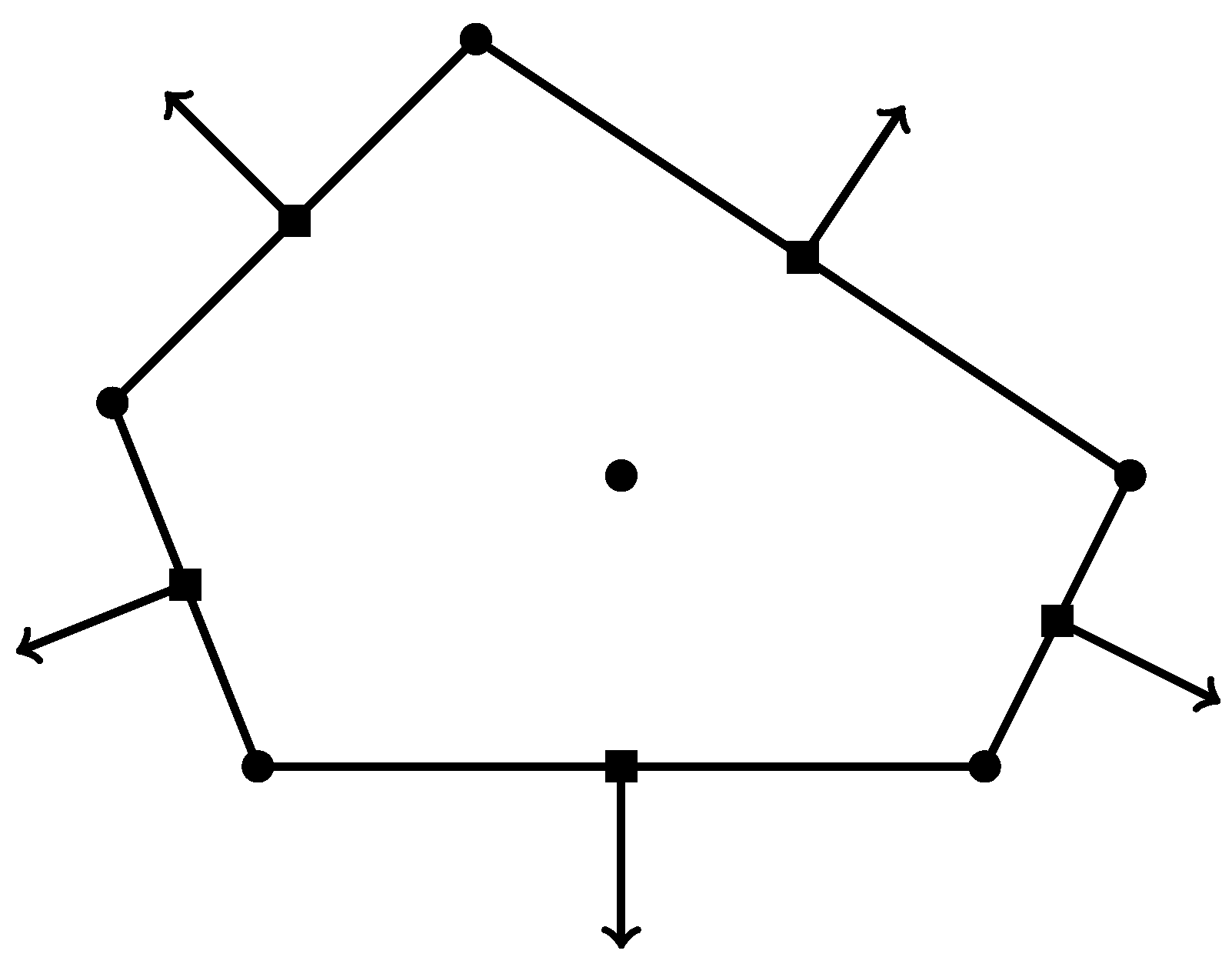
Figure 2 illustrates the DOFs in (13)–(16), and the total number of DOFs is given by

$$N_{\mathrm{dof}}^{T,\mathrm{nc}}=3m+1.$$

Figure 2. The DOFs of the lowest-order $C^0$ nonconforming VE on $V_h^T$.

Lemma 2.

Assuming T is a convex polygon, the degrees of freedom in (13)–(16) are unisolvent for $V_h^T$.

Proof. 

Since the dimension of $V_h^T$ equals the total number of DOFs in (13)–(16), showing that all DOFs uniquely determine a function in $V_h^T$ is sufficient to prove uniqueness. Assuming that all DOFs of v are zero, it is sufficient for us to prove that v is equal to 0. For each edge e of the element T, we know that ${v|}_e\in {\mathbb{P}}_2\left(e\right)$ and ${v|}_{\partial T}\in C^0(\partial T)$. And since the degrees of freedom in (13) and (14) are all zero, we can derive that ${v|}_{\partial T}=0$. Using the twice Green’s formula, we have

$${\int }_T{|\Delta v|}^{2}dx={\int }_{T}v{\Delta }^{2}vdx+{\int }_{\partial T}\Delta v{\displaystyle \frac{\partial v}{\partial {\mathit{n}}_T}}ds-{\int }_{\partial T}v{\displaystyle \frac{\partial \Delta v}{\partial {\mathit{n}}_T}}ds={\int }_{T}v{\Delta }^{2}vdx+{\int }_{\partial T}\Delta v{\displaystyle \frac{\partial v}{\partial {\mathit{n}}_T}}ds.$$

Since $V_h^T$ is defined in (12), it follows that ${\Delta }^{2}v\in {\mathbb{P}}_0\left(T\right)$ and ${\Delta v|}_e\in {\mathbb{P}}_0\left(e\right)$. Given that the degrees of freedom in (15) and (16) are all zero, the right-hand side of the above equation evaluates to zero. Consequently, we have $\Delta v=0$ on T. On the boundary of the element T, it holds that $v=0$, thus leading to the conclusion that $v\equiv 0$. □

The global construction of $V_h$. The global space for $C^0$ nonconforming virtual elements with $k=2$ is characterized by

$$V_h:=\{v\in H^{2,\mathrm{nc}}\left({\mathcal{T}}_h\right);v{|}_T\in V_h^T\forall T\in {\mathcal{T}}_h\}.$$

(17)

The global DOFs are as follows:

$$\begin{array}{cc}\hfill & •{\tilde{\mathrm{D}}}_1:\mathrm{The}\mathrm{value}\mathrm{of}\mathrm{the}\mathrm{function}v\mathrm{at}\mathrm{the}\mathrm{vertex}\mathrm{of}\mathrm{the}\mathrm{mesh};\hfill \end{array}$$

(18)

$$\begin{array}{cc}\hfill & •{\tilde{\mathrm{D}}}_2:\frac{1}{h_e}{\int }_{e}vds\mathrm{for}\mathrm{all}\mathrm{edges}\mathrm{of}\mathrm{the}\mathrm{mesh};\hfill \end{array}$$

(19)

$$\begin{array}{cc}\hfill & •{\tilde{\mathrm{D}}}_3:{\int }_e{\partial }_{\mathit{n}}vds\mathrm{for}\mathrm{all}\mathrm{edges}\mathrm{of}\mathrm{the}\mathrm{mesh};\hfill \end{array}$$

(20)

$$\begin{array}{cc}\hfill & •{\tilde{\mathrm{D}}}_4:\frac{1}{\left|T\right|}{\int }_{T}vdx\mathrm{for}\mathrm{all}\mathrm{elements}\mathrm{of}\mathrm{the}\mathrm{mesh}.\hfill \end{array}$$

(21)

For each element $T\in {\mathcal{T}}_h$, suppose that ${\chi }_i$ represents the operator corresponding to the i-th local degree of freedom, as defined in (13)–(16), where $i=1,2,\dots ,N_{\mathrm{dof}}^{T,\mathrm{nc}}$. The construction implies that for any sufficiently smooth function g, there exists a unique interpolation $g_I\in V_h^T$ satisfying

$${\chi }_i(g-g_I)=0,i=1,2,\dots ,N_{\mathrm{dof}}^{T,\mathrm{nc}}.$$

Subsequently, the following approximation results are valid.

Lemma 3

([28]). For every element $T\in {\mathcal{T}}_h$ and every function g belonging to the Sobolev space $H^s\left(T\right)$, where $2\le r\le 3$, there exist functions $g_I\in V_h^T$ and $g_{\pi }\in {\mathbb{P}}_2\left(T\right)$ satisfying

$$\parallel g-g_I{\parallel }_{m,T}\le C{h}^{r-m}{\left|g\right|}_{r,T},m=0,1,2,$$

(22)

$$\parallel g-g_{\pi }{\parallel }_{m,T}\le C{h}^{r-m}{\left|g\right|}_{r,T},m=0,1,2.$$

(23)

Construction of ${\mathcal{A}}_h$. Following the approach outlined in [28,38], we construct a discrete bilinear form ${\mathcal{A}}_h$ that is both symmetric and computable. Utilizing (6), we obtain

$$\begin{array}{cc}\hfill {\mathcal{A}}^T(p,v)& =-{\int }_T\nabla ·(\nabla ·ϵ\left(p\right))vdx-{\int }_{\partial T}\left(ϵ\left(p\right)\mathit{n}\right)·\nabla vds+{\int }_{\partial T}(\nabla ·ϵ\left(p\right))·\mathit{n}vds\hfill \end{array}$$

(24)

for any $p\in {\mathbb{P}}_2\left(T\right)$ and $v\in V_h^T$. Using the local DOF of v as defined in (13)–(16), the terms on the right-hand side of (24) can be computed straightforwardly.

Prior to establishing ${\mathcal{A}}_h(·,·)$, we initially introduce a projection operator ${\Pi }^T:V_h^T\to {\mathbb{P}}_2\left(T\right)\subset V_h^T$, defined as

$$\left\{\begin{array}{c}{\mathcal{A}}^T({\Pi }^T\eta ,q)={\mathcal{A}}^T(\eta ,q)\forall q\in {\mathbb{P}}_2\left(T\right)\forall \eta \in V_h^T,\hfill \\ \widehat{{\Pi }^T\eta }=\widehat{\eta },{\int }_{\partial T}\nabla {\Pi }^T\eta \mathrm{d}s={\int }_{\partial T}\nabla \eta \mathrm{d}s.\hfill \end{array}\right.$$

Here, we define the quasi-average $\widehat{\eta }$ as the average value computed from the values at the m vertices $b^i$ of T, given by

$$\widehat{\eta }=\frac{1}{m}\sum _{i=1}^m\eta \left(b^i\right).$$

Verification of the fact that

$${\Pi }^{T}v=v\forall v\in {\mathbb{P}}_2\left(T\right).$$

is straightforward. Furthermore, consider

$$S^T(v,w)=\sum _{i=1}^{N_{\mathrm{dof}}^{\mathrm{nc},T}}{h}_i^{-2}{\chi }_i\left(v\right){\chi }_i\left(w\right),$$

where $h_i$ represents the characteristic length associated with each degree of freedom ${\chi }_i$. Subsequently, we establish

$${\mathcal{A}}_h^T(u,v):={\mathcal{A}}^T({\Pi }^{T}u,{\Pi }^{T}v)+S^T(u-{\Pi }^{T}u,v-{\Pi }^{T}v)\forall u,v\in V_h^T.$$

(25)

We can observe that the bilinear form ${\mathcal{A}}_h^T$ satisfies the following properties:

•

Polynomial consistency: $\forall v_h\in V_h^T$,

$${\mathcal{A}}_h^T(v_h,p)={\mathcal{A}}^T(v_h,p)\forall p\in {\mathbb{P}}_k\left(T\right);$$

(26)

•

Stability: The constants ${\beta }_{*}>0$ and ${\beta }^{*}>0$ exist, which are independent of h and T, such that

$${\beta }_{*}{\mathcal{A}}^T(v_h,v_h)\le {\mathcal{A}}_h^T(v_h,v_h)\le {\beta }^{*}{\mathcal{A}}^T(v_h,v_h)\forall v_h\in V_h^T.$$

(27)

It should be emphasized that (3) and (4) remain valid for functions in $V_h^T$.

$$\begin{array}{cc}\hfill & {\mathcal{A}}^T(u_h,v_h)\le {\lambda }_1|u_h{|}_{2,T}{\left|v_h\right|}_{2,T}\forall u_h,v_h\in V_h^T,\hfill \\ \hfill & {\mathcal{A}}^T(v_h,v_h)\ge {\lambda }_2{\left|v_h\right|}_{2,T}^2\forall v_h\in V_h^T.\hfill \end{array}$$

Consider that ${|·|}_{2,h}$ defines a norm on the space $H^{2,\mathrm{nc}}\left({\mathcal{T}}_h\right)$ [38]. Moreover, (3) and (4) remain valid for functions in $H^{2,\mathrm{nc}}\left({\mathcal{T}}_h\right)$. The stability (27) of ${\mathcal{A}}_h(·,·)$ and the continuity requirement (3) of $\mathcal{A}(·,·)$ straightforwardly imply the continuity

$$\begin{array}{c}\hfill {\mathcal{A}}_h^T(u_h,v_h)\le {\beta }^{*}{\lambda }_1|u_h{|}_{2,T}{\left|v_h\right|}_{2,T}\forall u_h,v_h\in V_h^T.\end{array}$$

(28)

Define the bilinear form

$${\mathcal{A}}_h(u_h,v_h)=\sum _{T\in {\mathcal{T}}_h}{\mathcal{A}}_h^T(u_h,v_h).$$

(29)

By the same argument as in [28], the stability (27) and continuity (28) lead to

$$\begin{array}{cc}\hfill {\mathcal{A}}_h(u_h,v_h)\le & {\beta }^{*}{\lambda }_1|u_h{|}_{2,h}{\left|v_h\right|}_{2,h}\forall u_h,v_h\in V_h,\hfill \end{array}$$

(30)

$$\begin{array}{cc}\hfill {\mathcal{A}}_h(v_h,v_h)\ge & {\beta }_{*}{\lambda }_2{\left|v_h\right|}_{2,h}^2\forall v_h\in V_h.\hfill \end{array}$$

(31)

Construction of the right-hand side $l_h$.

Define $l_h\in {\left(V_h\right)}^{\prime }$ such that

$$\begin{array}{c}\hfill ⟨l_h,v_h⟩=\sum _{T\in {\mathcal{T}}_h}{\int }_T{P}_0^{T}l\widehat{v_h}dx\forall v_h\in V_h.\end{array}$$

Consequently, the approximation property is given by

$$\parallel l-l_h{\parallel }_{{\left(V_h\right)}^{\prime }}\le Ch{\parallel l\parallel }_0,$$

(32)

where $\parallel l-l_h{\parallel }_{{\left(V_h\right)}^{\prime }}=\underset{v_h\in V_h}{sup}\frac{(l,v_h)-⟨l_h,v_h⟩}{|v_h{|}_{2,h}}$.

3.2. $C^0$ Nonconforming VE Scheme

After establishing the VE space, ${\mathcal{A}}_h$ and $l_h$, we can now introduce the $C^0$ nonconforming VE scheme for solving the plate obstacle problem, denoted as Target Problem $\mathcal{T}$.

Target Problem ${\mathcal{T}}_h$. Find $u_h\in {\mathcal{S}}_h$ such that

$${\mathcal{A}}_h(u_h,v_h-u_h)\ge ⟨l_h,v_h-u_h⟩\forall v_h\in {\mathcal{S}}_h,$$

(33)

where

$${\mathcal{S}}_h=\{v_h\in V_h;{\tilde{\mathrm{D}}}_i\left(v_h\right)\ge {\tilde{\mathrm{D}}}_i\left(\xi \right),i=1,2,4.\}.$$

(34)

4. Error Estimation

In this section, we derive a priori error estimation of the $C^0$ nonconforming VEM applied to solve for Target Problem ${\mathcal{T}}_h$.

Theorem 1.

Let $u\in H^3(\Omega )\cap H_0^2(\Omega )$ be the solution of Target Problem $\mathcal{T}$and $u_h$ be the solution of Target Problem ${\mathcal{T}}_h$. Assuming that $\xi \in H^3(\Omega )$, $l\in L^2(\Omega )$ and $\nabla ·(\nabla ·ϵ)\in L^2(\Omega )$, we have

$$|u-u_h{|}_{2,h}\le Ch,$$

(35)

where the constant C depends only on $l,\xi ,u$ and constants ${\lambda }_1,{\lambda }_2,{\beta }_{*},{\beta }^{*}$.

Proof. 

Decompose the error e into two components $e_I$ and $e_h$:

$$e=u-u_h=u-u_I+u_I-u_h=e_I+e_h,$$

where $e_I$ and $e_h$ are defined accordingly. By applying (26), (31) and (33),

$$\begin{array}{cc}\hfill {\beta }_{*}{\lambda }_2{\left|e_h\right|}_{2,h}^2\le & {\mathcal{A}}_h(e_h,e_h)={\mathcal{A}}_h(u_I,e_h)-{\mathcal{A}}_h(u_h,e_h)\le {\mathcal{A}}_h(u_I,e_h)-⟨l_h,e_h⟩\hfill \\ \hfill =& \sum _{T\in {\mathcal{T}}_h}\left({{\mathcal{A}}_h}^T(u_I-u_{\pi },e_h)+{{\mathcal{A}}_h}^T(u_{\pi },e_h)\right)-⟨l_h,e_h⟩\hfill \\ \hfill =& \sum _{T\in {\mathcal{T}}_h}\left({{\mathcal{A}}_h}^T(u_I-u_{\pi },e_h)+{\mathcal{A}}^T(u_{\pi },e_h)\right)-⟨l_h,e_h⟩\hfill \\ \hfill =& \sum _{T\in {\mathcal{T}}_h}\left({{\mathcal{A}}_h}^T(u_I-u_{\pi },e_h)+{\mathcal{A}}^T(u_{\pi }-u,e_h)\right)+\sum _{T\in {\mathcal{T}}_h}{\mathcal{A}}^T(u,e_h)-(l,e_h)\hfill \\ \hfill & +(l,e_h)-⟨l_h,e_h⟩\hfill \\ \hfill =& R_1+R_2+R_3,\hfill \end{array}$$

(36)

where

$$\begin{array}{cc}\hfill & R_1=\sum _{T\in {\mathcal{T}}_h}({{\mathcal{A}}_h}^T(u_I-u_{\pi },e_h)+{\mathcal{A}}^T(u_{\pi }-u,e_h)),\hfill \end{array}$$

(37)

$$\begin{array}{cc}\hfill & R_2=(l,e_h)-⟨l_h,e_h⟩,\hfill \end{array}$$

(38)

$$\begin{array}{cc}\hfill & R_3=\sum _{T\in {\mathcal{T}}_h}{\mathcal{A}}^T(u,e_h)-(l,e_h).\hfill \end{array}$$

(39)

Applying the continuity of the bilinear forms ${{\mathcal{A}}_h}^T$ and ${\mathcal{A}}^T$, we have

$$R_1\le {\lambda }_1({\beta }^{*}|u_I-u_{\pi }{|}_{2,h}|e_h{|}_{2,h}+|u_{\pi }{-u|}_{2,h}|e_h{|}_{2,h}).$$

Using (32), we find

$$R_2\le \parallel l-l_h{\parallel }_{{\left(V_h\right)}^{\prime }}{\left|e_h\right|}_{2,h}.$$

Thus, we obtain

$$|e_h{|}_{2,h}^2\le C\left(|u_I-u_{\pi }{|}_{2,h}+|u_{\pi }{-u|}_{2,h}+{\parallel l-l_h\parallel }_{{\left(V_h\right)}^{\prime }}\right){\left|e_h\right|}_{2,h}+R_3.$$

(40)

Additionally, we have

$$|u-u_I{|}_{2,h}+|u-u_{\pi }{|}_{2,h}+{\parallel l-l_h\parallel }_{{\left({\tilde{V}}_h\right)}^{\prime }}\le Ch.$$

To estimate $R_3$, we partition ${\mathcal{T}}_h$ into the following three parts:

$$\begin{array}{cc}\hfill {\mathcal{T}}_h^{+}& =\{T\in {\mathcal{T}}_h:T\subset {\Omega }^{+}\},\hfill \\ \hfill {\mathcal{T}}_h^0& =\{T\in {\mathcal{T}}_h:T\subset {\Omega }^0\},\hfill \\ \hfill {\mathcal{T}}_h^b& ={\mathcal{T}}_h\setminus ({\mathcal{T}}_h^{+}\cup {\mathcal{T}}_h^0),\hfill \end{array}$$

where ${\mathcal{T}}_h^0$ denotes the set of elements in the contact domain and ${\mathcal{T}}_h^{+}$ signifies the set of all elements in the non-contact domain.

By (6), we have

$$\begin{array}{cc}\hfill R_3=& -\sum _{T\in {\mathcal{T}}_h}{\int }_Tϵ:{\nabla }^2{e}_{h}dx-(l,e_h)\hfill \\ \hfill =& \sum _{T\in {\mathcal{T}}_h}{\int }_{\partial T}{e}_h{\mathit{n}}_T·(\nabla ·ϵ)ds-\sum _{T\in {\mathcal{T}}_h}{\int }_T{e}_h\nabla ·(\nabla ·ϵ)dx\hfill \\ \hfill & -\sum _{T\in {\mathcal{T}}_h}{\int }_{\partial T}\left(ϵ{\mathit{n}}_T\right)·\nabla e_{h}ds-(l,e_h)\hfill \\ \hfill =& E_1+E_2+E_3,\hfill \end{array}$$

(41)

where

$$\begin{array}{cc}\hfill & E_1=\sum _{e\in {\mathcal{D}}_h}{\int }_e{e}_h[{\mathit{n}}_e·(\nabla ·ϵ)]ds,\hfill \end{array}$$

(42)

$$\begin{array}{cc}\hfill & E_2=-\sum _{T\in {\mathcal{T}}_h}{\int }_{\partial T}\left(ϵ{\mathit{n}}_T\right)·\nabla e_{h}ds=-\sum _{e\in {\mathcal{D}}_h}{\int }_eϵ{\mathit{n}}_e·[\nabla e_h]ds,\hfill \end{array}$$

(43)

$$\begin{array}{cc}\hfill & E_3={\int }_{\Omega }\mu e_{h}ds.\hfill \end{array}$$

(44)

Here, we denote $\mu =-\nabla ·(\nabla ϵ)-l$.

We now proceed to estimate $E_1$. Given $u\in H^3(\Omega ),\nabla ·ϵ\in L^2(\Omega )$, and $\nabla ·(\nabla ·ϵ)=-l\in L^2(\Omega )$, we can infer that $\nabla ·ϵ\in H\left(\mathrm{div}\right)$; consequently, $[{\mathit{n}}_e·(\nabla ·ϵ)]=0$ on ${{\mathcal{D}}_h}^i$. Additionally, since $e_h=0$ on $\Gamma$, we have $E_1$=0.

Next, we analyze $E_2$. Given $u\in H^3(\Omega )$, we have $ϵ\in {\left[H^1(\Omega )\right]}^{2\times 2}$, leading to $\left[ϵ{\mathit{n}}_e\right]=0$ for all $e\in {{\mathcal{D}}_h}^i$. Since $e_h{|}_e\in {\mathbb{P}}_2\left(e\right)$, ${\partial }_{\mathit{t}}{e}_h$ is continuous. Thus,

$$\begin{array}{c}\hfill E_2=-\sum _{T\in {\mathcal{T}}_h}{\int }_{\partial T}\left(ϵ{\mathit{n}}_T\right)·\nabla e_{h}ds=-\sum _{e\in {\mathcal{D}}_h}{\int }_eϵ{\mathit{n}}_e·[\nabla e_h]ds=-\sum _{e\in {\mathcal{D}}_h}{\int }_e{ϵ}_n\left[{\partial }_{\mathit{n}}{e}_h\right]ds.\end{array}$$

(45)

Following the argument in [28] and considering $e_h\in V_h\subset H^{2,\mathrm{nc}}\left({\mathcal{T}}_h\right)$, we find

$${\int }_e\left[{\partial }_{\mathit{n}}{e}_h\right]ds=0\forall e\in {\mathcal{D}}_h,$$

which yields

$$\begin{array}{cc}\hfill {\int }_e{ϵ}_n\left[{\partial }_{\mathit{n}}{e}_h\right]ds& ={\int }_e({ϵ}_n-P_0^T{ϵ}_n)[{\partial }_{\mathit{n}}{e}_h-P_0^e\left({\partial }_{\mathit{n}}{e}_h\right)]ds\hfill \\ \hfill & \le \parallel {ϵ}_n-P_0^T{ϵ}_n{\parallel }_{0,e}{\parallel [{\partial }_{\mathit{n}}{e}_h-P_0^e\left({\partial }_{\mathit{n}}{e}_h\right)]\parallel }_{0,e}.\hfill \end{array}$$

Here, $P_m^T$ represents the $L^2$-projection onto the space of m-order polynomials on the element T. Utilizing the standard approximation estimates [46], for each edge $e\in {\mathcal{D}}_h$, we obtain

$$\begin{array}{cc}\hfill \parallel {ϵ}_n-P_0^T{ϵ}_n{\parallel }_{0,e}& \le C{h}_T^{\frac{1}{2}}{\left|u\right|}_{3,{\omega }_e},\hfill \\ \hfill \parallel [{\partial }_{\mathit{n}}{e}_h-P_0^e\left({\partial }_{\mathit{n}}{e}_h\right)]{\parallel }_{0,e}& \le C{h}_T^{\frac{1}{2}}{\left|e_h\right|}_{2,{\omega }_e}.\hfill \end{array}$$

This implies

$$\sum _{e\in {{\mathcal{D}}_h}^i}{\int }_e(-{ϵ}_n)\left[{\partial }_{\mathit{n}}{e}_h\right]ds\le {Ch\left|u\right|}_3{\left|e_h\right|}_{2,h}.$$

(46)

Let us analyze $E_3$ step by step. We start with its definition:

$$E_3=\sum _{T\in {\mathcal{T}}_h}{\int }_T\mu (u_I-u_h)dx=A_1+A_2+A_3,$$

(47)

where

$$A_1=\sum _{T\in {\mathcal{T}}_h^{+}}{\int }_T\mu (u_I-u_h)dx,$$

$$A_2=\sum _{T\in {\mathcal{T}}_h^0}{\int }_T\mu (u_I-u_h)dx,$$

$$A_3=\sum _{T\in {\mathcal{T}}_h^b}{\int }_T\mu (u_I-u_h)dx.$$

We can show that $A_1=0$ by Lemma 1. In order to estimate $A_2$, we define

$$P_0^{T}v:=\frac{1}{\left|T\right|}{\int }_{T}vdx,R_0^{T}v:=v-P_0^{T}v.$$

Since $\mu \ge 0$, we have $P_0^T\mu \ge 0$. Given the definition of ${\mathcal{S}}_h$, we know that ${\mathrm{D}}_i\left(u_h\right)\ge {\mathrm{D}}_i\left(\xi \right),i=1,2,4.$ Additionally, ${\mathrm{D}}_i\left({\xi }_h\right)={\mathrm{D}}_i\left(\xi \right)$, and ${\displaystyle \frac{1}{\left|T\right|}{\int }_{T}vdx}$ represents the fourth type of degrees of freedom. Thus, ${\displaystyle {\int }_T({\xi }_I-u_h)dx\le 0}$. This leads to

$$\begin{array}{cc}\hfill {\int }_T\mu ({\xi }_I-u_h)dx& \le {\int }_T{R}_0^T\mu R_0^T({\xi }_I-u_h)dx\hfill \\ \hfill & \le \parallel R_0^T{\mu \parallel }_{0,T}{\parallel R_0^T({\xi }_I-u_h)\parallel }_{0,T}.\hfill \end{array}$$

Note that in $T\in {\mathcal{T}}_h^0$, where $u=\xi$, and given $\xi \in H^3(\Omega )$, we have

$$\begin{array}{cc}\hfill {\int }_T\mu ({\xi }_I-u_h)dx& \le \parallel R_0^T{\mu \parallel }_{0,T}{\parallel R_0^T({\xi }_I-u_h)\parallel }_{0,T}\hfill \\ \hfill & \le C{h}_T{\parallel \mu \parallel }_{0,T}{|{\xi }_I-u_h|}_{1,T}\hfill \\ \hfill & \le C{h}_T{\parallel \mu \parallel }_{0,T}\left(\right|{\xi }_I{-\xi |}_{1,T}+|\xi -u_h{|}_{1,T})\hfill \\ \hfill & \le C{h}_T{\parallel \mu \parallel }_{0,T}(h_T^2{\left|\xi \right|}_{3,T}+|u-u_h{|}_{1,T}),\hfill \end{array}$$

this implies

$$\begin{array}{cc}\hfill A_2& =\sum _{T\in {\mathcal{T}}_h^0}{\int }_T\mu (u_I-u_h)dx=\sum _{T\in {\mathcal{T}}_h^0}{\int }_T\mu ({\xi }_I-u_h)dx\hfill \\ \hfill & \le {Ch\parallel \mu \parallel }_0\left(h^2{\left|\xi \right|}_3+{|u-u_h|}_{1,h}\right)\hfill \\ \hfill & \le {Ch\parallel \mu \parallel }_0\left(h^2{\left|\xi \right|}_3+{|u-u_h|}_{2,h}\right).\hfill \end{array}$$

(48)

Now, let us consider the last term

$$\begin{array}{cc}\hfill A_3& =\sum _{T\in {\mathcal{T}}_h^b}\left({\int }_T\mu (u_I-u+\xi -{\xi }_I)dx+{\int }_T\mu (u-\xi )dx+{\int }_T\mu ({\xi }_I-u_h)dx\right)\hfill \\ \hfill & =\sum _{T\in {\mathcal{T}}_h^b}\left({\int }_T\mu [{(u-\xi )}_I-(u-\xi )]dx+{\int }_T\mu ({\xi }_I-u_h)dx\right)\hfill \\ \hfill & =A_{3,1}+A_{3,2},\hfill \end{array}$$

(49)

where

$$\begin{array}{cc}\hfill A_{3,1}=& \sum _{T\in {\mathcal{T}}_h^b}{\int }_T\mu [{(u-\xi )}_I-(u-\xi )]dx,\hfill \\ \hfill A_{3,2}=& \sum _{T\in {\mathcal{T}}_h^b}{\int }_T\mu ({\xi }_I-u_h)dx.\hfill \end{array}$$

We can estimate $A_{3,1}$ as follows:

$$\begin{array}{cc}\hfill & {\int }_T\mu [{(u-\xi )}_I-(u-\xi )]dx\le C{h}_T^3{\parallel \mu \parallel }_{0,T}{|u-\xi |}_{3,T}.\hfill \end{array}$$

(50)

Let us now analyze $A_{3,2}$

$$\begin{array}{cc}\hfill {\int }_T\mu ({\xi }_I-u_h)dx& \le {\int }_T{R}_0^T\mu R_0^T({\xi }_I-u_h)dx\hfill \\ \hfill & \le {\int }_T{R}_0^T\mu R_0^T({\xi }_I-\xi )+R_0^T\mu R_0^T(\xi -u)+R_0^T\mu R_0^T(u-u_h)dx.\hfill \end{array}$$

(51)

We estimate each of the three terms as follows:

$$\begin{array}{cc}\hfill & {\int }_T{R}_0^T\mu R_0^T({\xi }_I-\xi )dx\le C{h}_T{\parallel \mu \parallel }_{0,T}|{\xi }_I{-\xi |}_{1,T}\le C{h}_T^3{\parallel \mu \parallel }_{0,T}{\left|\xi \right|}_{3,T},\hfill \end{array}$$

(52)

$$\begin{array}{cc}\hfill & {\int }_T{R}_0^T\mu R_0^T(u-u_h)dx\le {\parallel \mu \parallel }_{0,T}\parallel R_0^T(u-u_h){\parallel }_{0,T}\le C{h}_T{\parallel \mu \parallel }_{0,T}{|u-u_h|}_{1,T},\hfill \end{array}$$

(53)

$$\begin{array}{cc}\hfill & {\int }_T{R}_0^T\mu R_0^T(\xi -u)dx\le \parallel R_0^T{\mu \parallel }_{0,T}\parallel R_0^T{(\xi -u)\parallel }_{0,T}\le C{h}_T{\parallel \mu \parallel }_{0,T}{|\xi -u|}_{1,T}.\hfill \end{array}$$

(54)

By the embedding theorem,

$$\nabla (\xi -u)\in H^2\hookrightarrow C^0,$$

and there exists $D\subset T$, which means that $\left(D\right)>0$ such that

$$\begin{array}{c}\hfill \xi =uD,\\ \hfill \nabla \xi =\nabla uD.\end{array}$$

According to the Bramble–Hilbert lemma, we have ${|\xi -u|}_{1,T}\le C{h}_T^2{|\xi -u|}_{3,T}$, so

$${\int }_T{R}_0^T\mu R_0^T(\xi -u)dx\le C{h}_T^3{\parallel \mu \parallel }_{0,T}{|\xi -u|}_{3,T}.$$

(55)

Combining (47)–(55), we find

$$E_3\le C\left(h^3{\parallel \mu \parallel }_0\left({\left|u\right|}_3+{\left|\xi \right|}_3\right)+{h\parallel \mu \parallel }_0{|u-u_h|}_{2,h}\right),$$

which implies

$$R_3\le C\left({h\left|u\right|}_3|e_h{|}_{2,h}+h^3{\parallel \mu \parallel }_0\left({\left|u\right|}_3+{\left|\xi \right|}_3\right)+{h\parallel \mu \parallel }_0{|u-u_h|}_{2,h}\right),$$

and thus (40) can be expressed as

$$\begin{array}{cc}\hfill |e_h{|}_{2,h}^2\le & C\left(|u_I-u_{\pi }{|}_{2,h}+|u_{\pi }{-u|}_{2,h}+\parallel l-l_h{\parallel }_{{\left(V_h\right)}^{\prime }}+h{\left|u\right|}_3\right){\left|e_h\right|}_{2,h}\hfill \\ \hfill & +C{h}^3{\parallel \mu \parallel }_0\left({\left|u\right|}_3+{\left|\xi \right|}_3\right)+{Ch\parallel \mu \parallel }_0{|u-u_h|}_{2,h}.\hfill \end{array}$$

Finally, applying the triangle inequality allows us to derive (35). □

5. Numerical Example

In this section, we conduct a numerical experiment to verify the accuracy and convergence properties of the $C^0$ nonconforming VEM that we proposed above. For details on how to implement the VEM, please refer to [47].

Example 1.

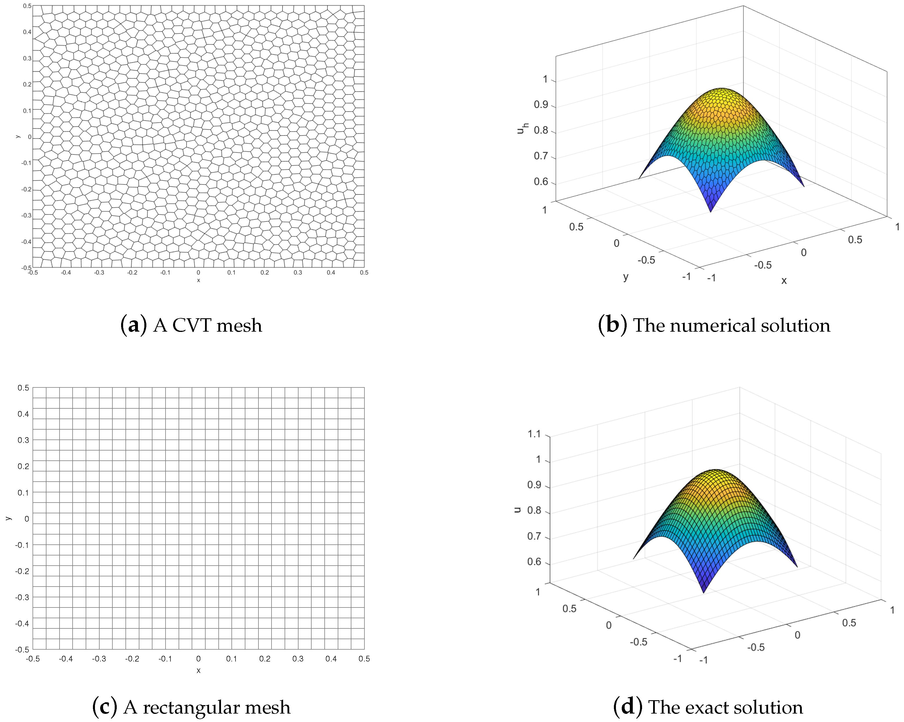
We consider the following setup for the Kirchhoff plate obstacle problem (1): $\Omega =(-0.5,0.5)\times (-0.5,0.5)$, $\nu =0.3$, $l=0$, $\xi \left(x\right)=1-{\left|x\right|}^2$. The exact solution for this problem is given by

$$u\left(x\right)=\left\{\begin{array}{ccc}\hfill & C_1{\left|x\right|}^2\left(\ln \right|x\left|\right)+C_2{\left|x\right|}^2+C_3\left(\ln \right|x\left|\right)+C_4,\hfill & \hfill r_0<\left|x\right|<2\\ \hfill & 1-{\left|x\right|}^2,\hfill & \hfill \left|x\right|\le r_0\end{array},\right.$$

(56)

where $r_0\approx 0.18134452$, $C_1\approx 0.52504063$, $C_2\approx -0.62860904$, $C_3\approx 0.01726640$, and $C_4\approx 1.04674630$.

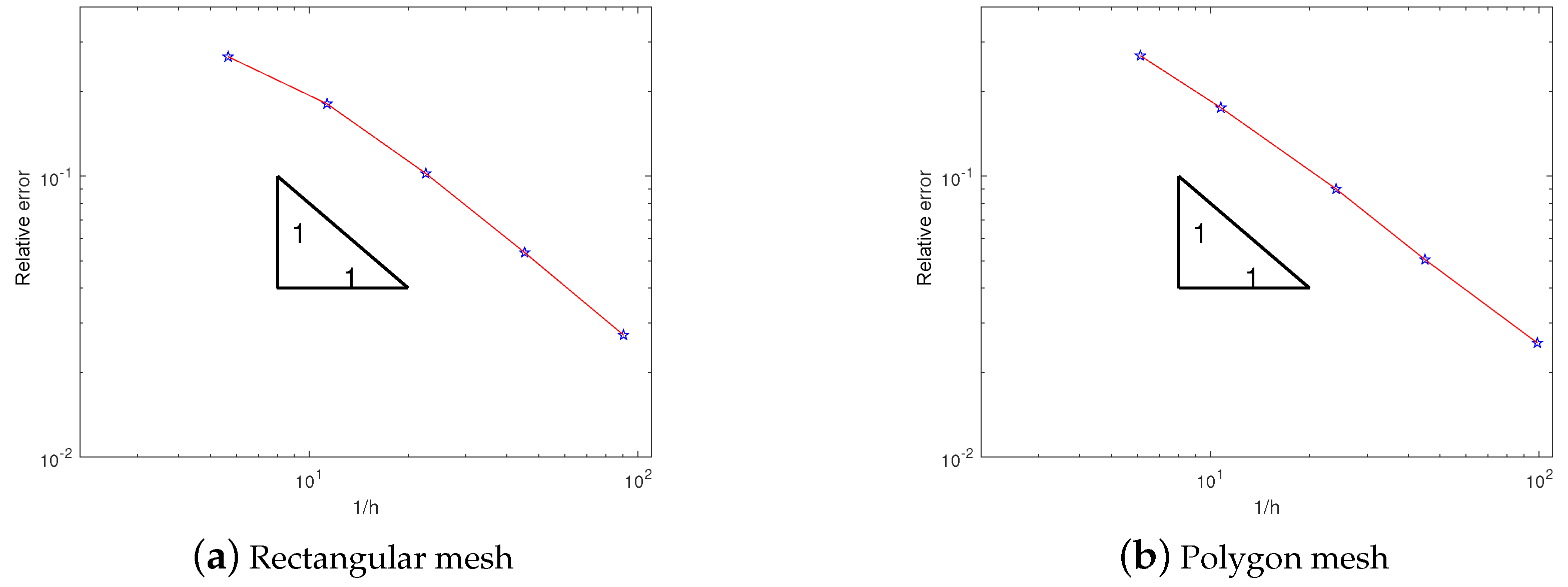
We determine the convergence orders by discretizing the problem using square meshes with $h=\sqrt{2}/2^n$ ($n=3,\cdots ,7$) and polygon meshes. The results in Table 1 and Table 2 indicate that the $C^0$ nonconforming method exhibits linear convergence, consistent with the findings of Theorem 1. Here, the $H^2$ relative error is computed as

$${\left(\frac{{\mathcal{A}}_h(u_I-u_h,u_I-u_h)}{{\mathcal{A}}_h(u_I,u_I)}\right)}^{1/2}.$$

Table 1. Convergence orders of $H^2$ relative errors on square meshes.

h	$\sqrt{2}/2^3$	$\sqrt{2}/2^4$	$\sqrt{2}/2^5$	$\sqrt{2}/2^6$	$\sqrt{2}/2^7$
${\mathit{H}}^{\mathbf{2}}$relative error	$2.587\times {10}^{-1}$	$1.787\times {10}^{-1}$	$1.019\times {10}^{-1}$	$5.343\times {10}^{-2}$	$2.720\times {10}^{-2}$
Convergence order	-	$0.534$	$0.810$	$0.931$	$0.974$

Table 2. Convergence orders of $H^2$ relative errors on polygonal meshes.

h	$1.636\times {10}^{-1}$	$9.306\times {10}^{-2}$	$4.146\times {10}^{-2}$	$2.223\times {10}^{-2}$	$1.011\times {10}^{-2}$
${\mathit{H}}^{\mathbf{2}}$relative error	$2.872\times {10}^{-1}$	$1.973\times {10}^{-1}$	$1.124\times {10}^{-1}$	$5.920\times {10}^{-2}$	$3.004\times {10}^{-2}$
Convergence order	-	$0.665$	$0.706$	$1.029$	$0.861$

Additionally, we also provide graphs corresponding to Table 1 and Table 2, as shown in Figure 3. The results further validate the linear convergence of the $C^0$ nonconforming VEM for $k=2$, aligning with the theoretical analysis in Theorem 1. In Figure 4, we present a surface diagram depicting the numerical solution obtained from a general polygonal mesh. The numerical solution obtained from the polygonal mesh closely aligns with the real solution on a uniformly divided rectangular mesh at the same location, indicating the effective use of virtual elements in general polygonal mesh computation.

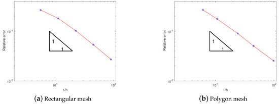
Figure 3. Relative errors of rectangular mesh and polygon mesh.

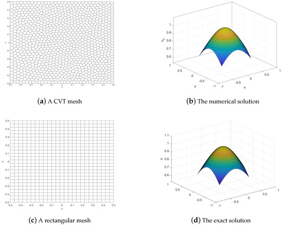
Figure 4. The numerical solution and exact solution.

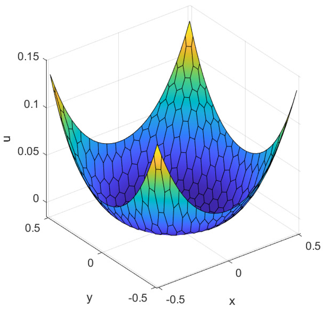
Importantly, in Figure 5, we also plot the numerical solution $u_h$ minus the value of the obstacle function $\xi$ at each point. In these figures, we can observe that the value of the numerical solution $u_h$ is greater than the value of $\xi$, which is consistent with the constraints of our VI problem (1).

Figure 5. The numerical solution minus the value of the obstacle function $\xi$.

6. Conclusions

In this paper, we investigate a novel $C^0$ nonconforming VEM for solving the Kirchhoff plate obstacle problem, which is formulated as a fourth-order variational inequality of the first kind. Our approach introduces new internal degrees of freedom to address the limitations of the traditional lowest-order $C^0$ nonconforming VEM, leading to improved error analysis and enhanced intuitiveness. Importantly, our method naturally satisfies the constraints of the obstacle problem and achieves optimal convergence in error estimates. Future work will focus on extending the method to handle different boundary conditions and exploring more efficient VEMs.

References

- Niiranen, J.; Khakalo, S.; Balobanov, V.; Niemi, A. Variational formulation and isogeometric analysis for fourth-order boundary value problems of gradient-elastic bar and plane strain/stress problems. Comput. Methods Appl. Mech. Eng. 2016, 308, 182–211. [Google Scholar] [CrossRef]
- Niiranen, J.; Niemi, A. Variational formulations and general boundary conditions for sixth-order boundary value problems of gradientelastic Kirchhoff plates. Eur. J. Mech. A-Solid. 2017, 61, 164–179. [Google Scholar] [CrossRef]
- Reissner, E. The effect of transverse shear deformation on the bending of elastic plates. J. Appl. Mech. 1945, 12, 69–77. [Google Scholar] [CrossRef]
- Timoshenko, S.; Woinowsky-krieger, S. Theory of Plates and Shells; Springer: Berlin/Heidelberg, Germany; McGraw-Hill: New York, NY, USA, 1959. [Google Scholar]
- Swider, J.; Kudra, G. Application of Kirchhoff’s plate theory for design and analysis of stiffened plates. J. Theor. 2017, 55, 805–817. [Google Scholar]
- Shahba, A.; Yas, H. Application of Galerkin method in solving static and dynamic problems of Kirchhoff plates. J. Solid Mech. 2015, 7, 374–384. [Google Scholar]
- He, H.; Peng, J.G.; Li, H.Y. Iterative approximation of fixed point problems and variational inequality problems on Hadamard manifolds. UPB Bull. Ser. A 2022, 84, 25–36. [Google Scholar]
- Lions, J.L.; Stampacchia, G. Variational inequalities. Commun. Pure Appl. Math. 1967, 20, 493–519. [Google Scholar] [CrossRef]
- Ferris, M.C.; Pang, J.S. Engineering and economic applications of complementarity problems. SIAM Rev. 1997, 39, 669–713. [Google Scholar] [CrossRef]
- Meng, S.; Meng, F.; Zhang, F.; Li, Q.; Zhang, Y. Observer design method for nonlinear generalized systems with nonlinear algebraic constraints with applications. Automatica 2024, 162, 111512. [Google Scholar] [CrossRef]
- Shi, M.; Hu, W.; Li, M.; Zhang, J.; Song, X.; Sun, W. Ensemble regression based on polynomial regression-based decision tree and its application in the in-situ data of tunnel boring machine. Mech. Syst. Signal. Pract. 2023, 188, 110022. [Google Scholar] [CrossRef]
- Shi, M.; Lv, L.; Xu, L. A multi-fidelity surrogate model based on extreme support vector regression: Fusing different fidelity data for engineering design. Eng. Comput. 2023, 40, 473–493. [Google Scholar] [CrossRef]
- Li, B.; Guan, T.; Dai, L.; Duan, G. Distributionally robust model predictive control with output feedback. IEEE Trans. Autom. Control 2023, 69, 3270–3277. [Google Scholar] [CrossRef]
- Zhou, X.; Liu, X.; Zhang, G.; Jia, L.; Wang, X.; Zhao, Z. An iterative threshold algorithm of log-sum regularization for sparse problem. IEEE. Trans. Circuits. Syst. Video Technol. 2023, 33, 4728–4740. [Google Scholar] [CrossRef]
- Zhang, H.; Xiang, X.; Huang, B.; Wu, Z.; Chen, H. Static homotopy response analysis of structure with random variables of arbitrary distributions by minimizing stochastic residual error. Comput. Struct. 2023, 288, 107153. [Google Scholar] [CrossRef]
- da Veiga, L.B.; Brezzi, F.; Cangiani, A.; Manzini, G.; Marini, L.D.; Russo, A. Basic principles of virtual element methods. Math. Models Methods Appl. Sci. 2013, 23, 199–214. [Google Scholar] [CrossRef]
- Li, J.; Liu, Y.; Lin, G. Implementation of a coupled FEM-SBFEM for soil-structure interaction analysis of large-scale 3D base-isolated nuclear structures. Comput. Geotech. 2023, 162, 105669. [Google Scholar] [CrossRef]
- Babu, B.; Patel, B.P. A new computationally efficient finite element formulation for nanoplates using second-order strain gradient Kirchhoff’s plate theory. Compos. Part. B-Eng. 2019, 168, 302–311. [Google Scholar] [CrossRef]
- Zhang, B.; Li, H.; Kong, L.; Zhang, X.; Feng, Z. Variational formulation and differential quadrature finite element for freely vibrating strain gradient Kirchhoff plates. Z. Angew. Math. Mech. 2021, 101, e202000046. [Google Scholar] [CrossRef]
- da Veiga, L.B.a.; Brezzi, F.; Marini, L.D. Virtual elements for linear elasticity problems. SIAM J. Numer. Anal. 2013, 51, 794–812. [Google Scholar] [CrossRef]
- Gain, A.L.; Talischi, C.; Paulino, G.H. On the virtual element method for three-dimensional elasticity problems on arbitrary polyhedral meshes. Comput. Methods Appl. Mech. Engrg. 2014, 282, 132–160. [Google Scholar] [CrossRef]
- Zhang, B.; Zhao, J.; Yang, Y.; Chen, S. The nonconforming virtual element method for elasticity problems. J. Comput. Phys. 2019, 378, 394–410. [Google Scholar] [CrossRef]
- Antonietti, P.F.; da Veiga, L.B.a.; Mora, D.; Verani, M. A stream function formulation of the Stokes problem for the virtual element method. SIAM J. Numer. Anal. 2014, 52, 386–404. [Google Scholar] [CrossRef]
- da Veiga, L.B.a.; Lovadina, C.; Vacca, G. Divergence free virtual elements for the Stokes problem on polygonal meshes. ESAIM Math. Model. Numer. Anal. 2017, 51, 509–535. [Google Scholar] [CrossRef]
- Zhao, J.; Zhang, B.; Mao, S.; Chen, S. The divergence-free nonconforming virtual element for the Stokes problem. SIAM J. Numer Anal. 2019, 57, 2730–2759. [Google Scholar] [CrossRef]
- Antonietti, P.F.; da Veiga, L.B.a.; Scacchi, S.; Verani, M. A C1 virtual element method for the Cahn-Hilliard equation with polygonal meshes. SIAM J. Numer. Anal. 2016, 54, 34–56. [Google Scholar] [CrossRef]
- Brezzi, F.; Marini, L.D. Virtual element methods for plate bending problems. Comput. Methods Appl. Mech. Engrg. 2013, 253, 455–462. [Google Scholar] [CrossRef]
- Zhao, J.; Chen, S.; Zhang, B. The nonconforming virtual element method for plate bending problems. Math. Models Methods Appl. Sci. 2016, 26, 1671–1687. [Google Scholar] [CrossRef]
- Antonietti, P.F.; Manzini, G.; Verani, M. The fully nonconforming virtual element method for biharmonic problems. Math. Models Methods Appl. Sci. 2018, 28, 199–214. [Google Scholar] [CrossRef]
- Zhao, J.; Zhang, B.; Chen, S.; Mao, S. The Morley-type virtual element for plate bending problems. J. Sci. Comput. 2018, 76, 610–629. [Google Scholar] [CrossRef]
- Feng, F.; Han, W.; Huang, J. Virtual element methods for elliptic variational inequalities of the second kind. J. Sci. Comput. 2019, 80, 60–80. [Google Scholar] [CrossRef]
- Feng, F.; Han, W.; Huang, J. Virtual element method for an elliptic hemivariational inequality with applications to contact mechanics. J. Sci. Comput. 2019, 81, 2388–2412. [Google Scholar] [CrossRef]
- Wang, F.; Wei, H. Virtual element method for simplified friction problem. Appl. Math. Lett. 2018, 85, 125–131. [Google Scholar] [CrossRef]
- Wang, F.; Wei, H.Y. Virtual element methods for the obstacle problem. IMA J. Numer. Anal. 2020, 40, 708–728. [Google Scholar] [CrossRef]
- Wang, F.; Wu, B.; Han, W. The virtual element method for general elliptic hemivariational inequalities. J. Comput. Appl. Math. 2021, 389, 113330. [Google Scholar] [CrossRef]
- Wriggers, P.; Rust, W.T.; Reddy, B.D. A virtual element method for contact. Comput. Mech. 2016, 58, 1039–1050. [Google Scholar] [CrossRef]
- Wu, B.; Wang, F.; Han, W. Virtual element method for a frictional contact problem with normal compliance. Commun. Nonlinear Sci. Numer. Simul. 2022, 107, 106125. [Google Scholar] [CrossRef]
- Wang, F.; Zhao, J. Conforming and nonconforming virtual element methods for a Kirchhoff plate contact problem. IMA J. Numer. Anal. 2021, 41, 1496–1521. [Google Scholar] [CrossRef]
- Qiu, J.; Zhao, J.; Wang, F. Nonconforming virtual element methods for the fourth-order variational inequalities of the first kind. J. Comput. Appl. Math. 2023, 425, 115025. [Google Scholar] [CrossRef]
- Duvaut, G.; Lions, J.L. Inequalities in Mechanics and Physics; Springer: Berlin, Germany, 1976. [Google Scholar]
- Wang, F.; Han, W.; Huang, J.; Zhang, T. Discontinuous Galerkin methods for an elliptic variational inequality of fourth-order. In Advances in Variational and Hemivariational Inequalities with Applications; Springer International: Cham, Switzerland, 2015; pp. 199–222. [Google Scholar]
- Atkinson, K.; Han, W. Theoretical Numerical Analysis: A Functional Analysis Framework; Springer: New York, NY, USA, 2009. [Google Scholar]
- Glowinski, R. Numerical Methods for Nonlinear Variational Problems; Springer: New York, NY, USA, 1984. [Google Scholar]
- Glowinski, R.; Lions, J.L.; Trèmolixexres, R. Numerical Analysis of Variational Inequalities; North-Holland: New York, NY, USA, 1981. [Google Scholar]
- da Veiga, L.B.a.; Lovadina, C. Stability analysis for the virtual element method. Math. Models Methods Appl. Sci. 2017, 27, 2557–2594. [Google Scholar] [CrossRef]
- Brenner, S.C.; Scott, L.R. Mathematical Theory of Finite Element Methods; Springer: New York, NY, USA, 1994. [Google Scholar]
- da Veiga, L.B.a.; Brezzi, F.; Marini, L.D.; Russo, A. The hitchhiker’s guide to the virtual element method. Math. Models Methods Appl. Sci. 2014, 24, 1541–1573. [Google Scholar] [CrossRef]
Disclaimer/Publisher’s Note: The statements, opinions and data contained in all publications are solely those of the individual author(s) and contributor(s) and not of MDPI and/or the editor(s). MDPI and/or the editor(s) disclaim responsibility for any injury to people or property resulting from any ideas, methods, instructions or products referred to in the content. |
© 2024 by the authors. Licensee MDPI, Basel, Switzerland. This article is an open access article distributed under the terms and conditions of the Creative Commons Attribution (CC BY) license (https://creativecommons.org/licenses/by/4.0/).