
A C0 Nonconforming Virtual Element Method for the Kirchhoff Plate Obstacle Problem

Abstract
1. Introduction
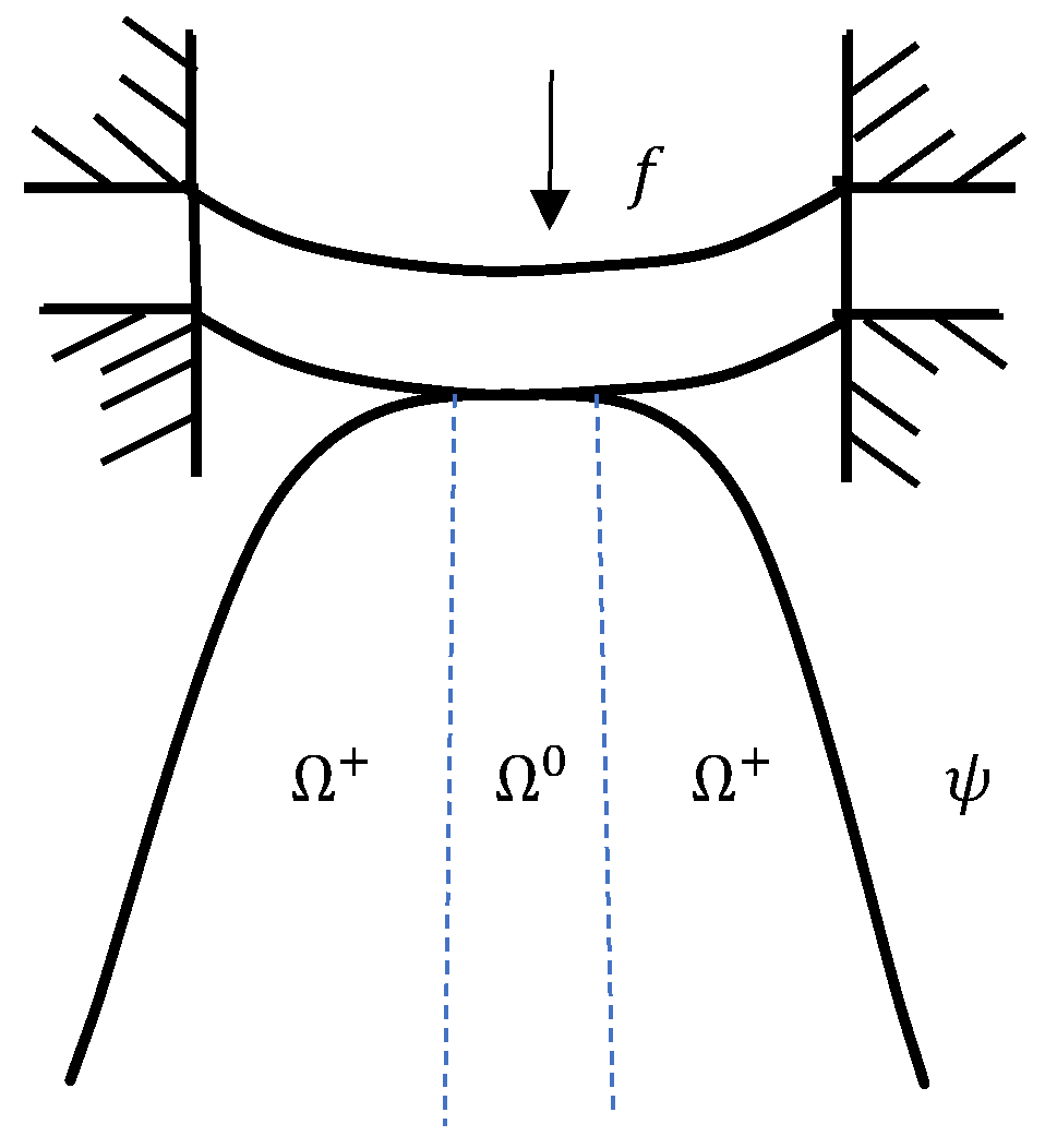
2. Plate Obstacle Model
2.1. Model Problem and Its Variational Inequality
2.2. Pointwise Relations of the Solution
3. Nonconforming VEM
- T is star-shaped in relation to a ball with a radius greater than or equal to ;
- The ratio of the shortest edge to is larger than .
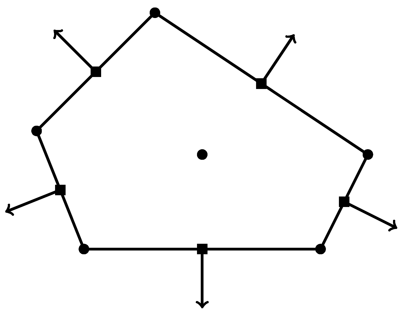
3.1. Construction of the Nonconforming VEM
- •
- Polynomial consistency: ,
- •
- Stability: The constants and exist, which are independent of h and T, such that
3.2. Nonconforming VE Scheme
4. Error Estimation
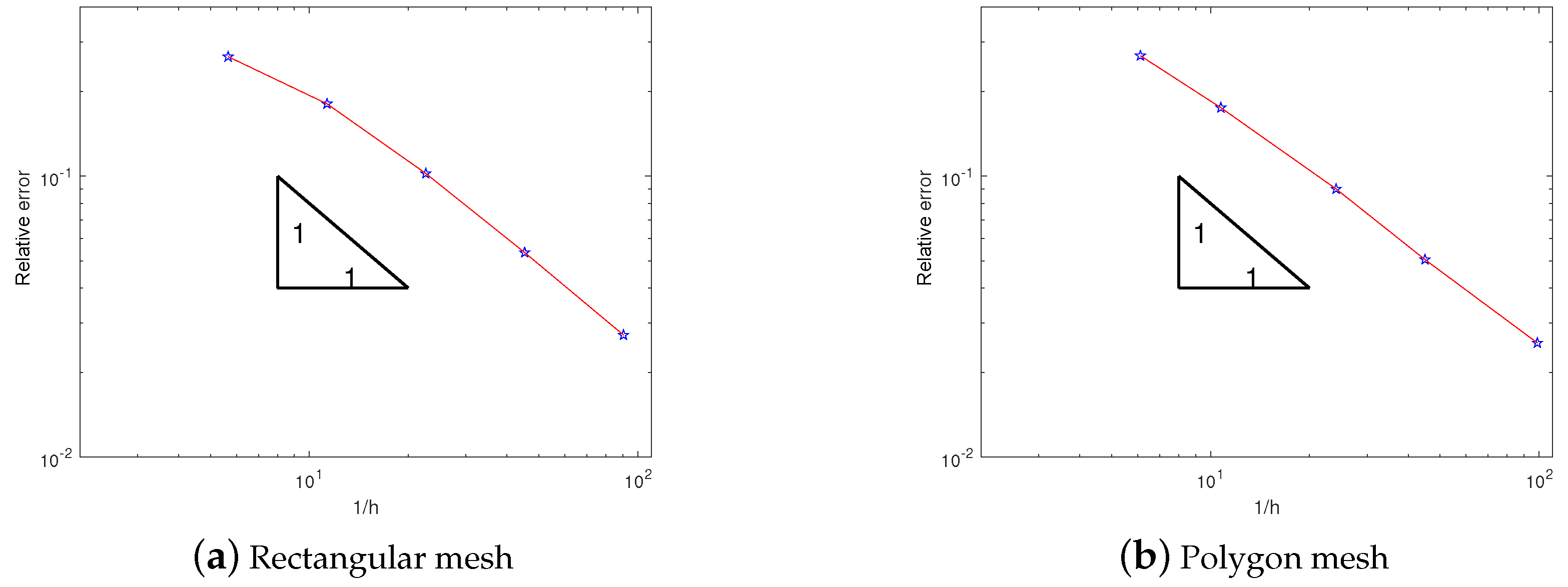
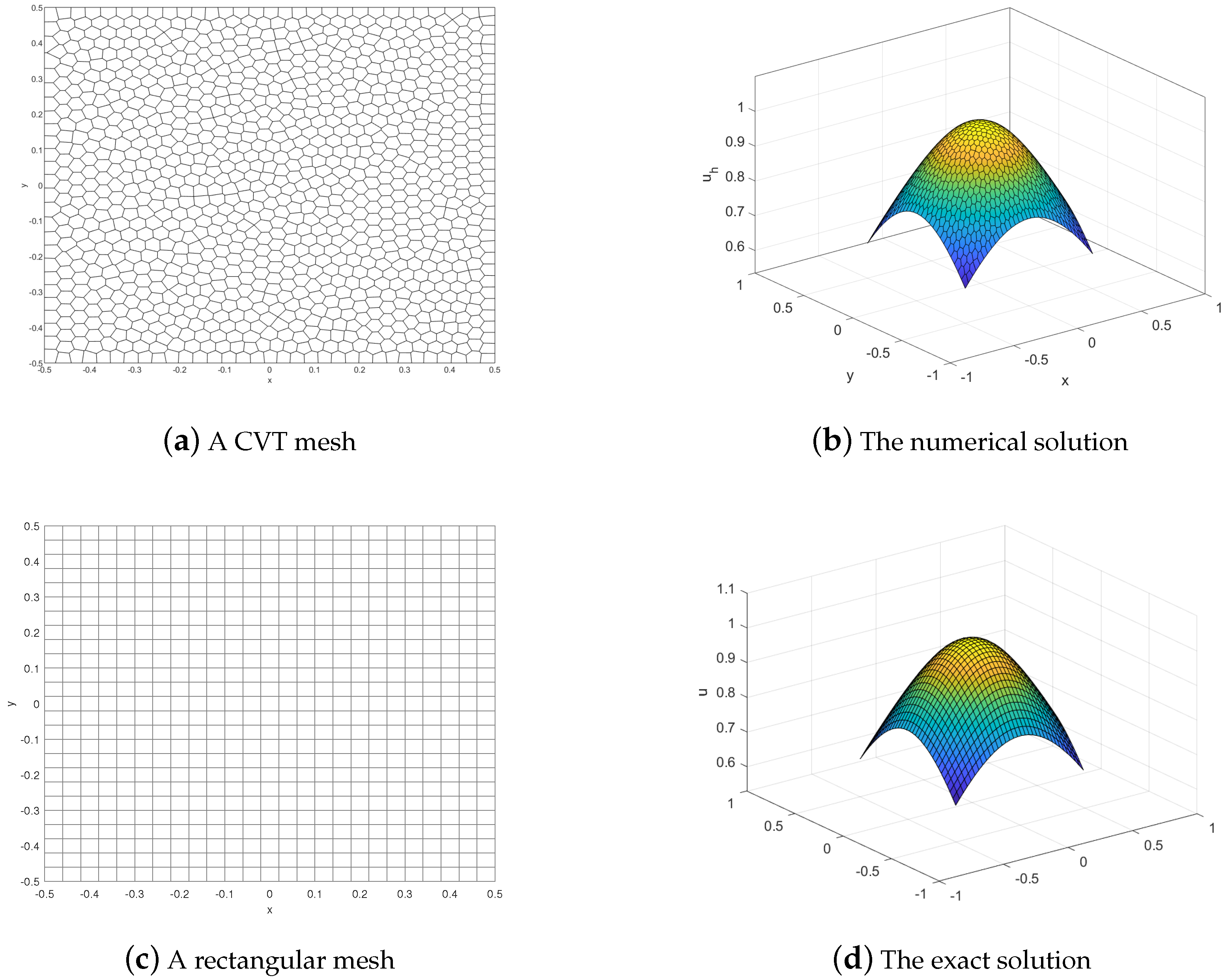
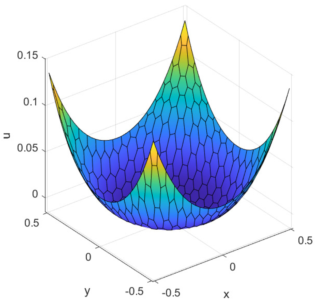
5. Numerical Example
6. Conclusions
Author Contributions
Funding
Data Availability Statement
Conflicts of Interest
References
- Niiranen, J.; Khakalo, S.; Balobanov, V.; Niemi, A. Variational formulation and isogeometric analysis for fourth-order boundary value problems of gradient-elastic bar and plane strain/stress problems. Comput. Methods Appl. Mech. Eng. 2016, 308, 182–211. [Google Scholar] [CrossRef]
- Niiranen, J.; Niemi, A. Variational formulations and general boundary conditions for sixth-order boundary value problems of gradientelastic Kirchhoff plates. Eur. J. Mech. A-Solid. 2017, 61, 164–179. [Google Scholar] [CrossRef]
- Reissner, E. The effect of transverse shear deformation on the bending of elastic plates. J. Appl. Mech. 1945, 12, 69–77. [Google Scholar] [CrossRef]
- Timoshenko, S.; Woinowsky-krieger, S. Theory of Plates and Shells; Springer: Berlin/Heidelberg, Germany; McGraw-Hill: New York, NY, USA, 1959. [Google Scholar]
- Swider, J.; Kudra, G. Application of Kirchhoff’s plate theory for design and analysis of stiffened plates. J. Theor. 2017, 55, 805–817. [Google Scholar]
- Shahba, A.; Yas, H. Application of Galerkin method in solving static and dynamic problems of Kirchhoff plates. J. Solid Mech. 2015, 7, 374–384. [Google Scholar]
- He, H.; Peng, J.G.; Li, H.Y. Iterative approximation of fixed point problems and variational inequality problems on Hadamard manifolds. UPB Bull. Ser. A 2022, 84, 25–36. [Google Scholar]
- Lions, J.L.; Stampacchia, G. Variational inequalities. Commun. Pure Appl. Math. 1967, 20, 493–519. [Google Scholar] [CrossRef]
- Ferris, M.C.; Pang, J.S. Engineering and economic applications of complementarity problems. SIAM Rev. 1997, 39, 669–713. [Google Scholar] [CrossRef]
- Meng, S.; Meng, F.; Zhang, F.; Li, Q.; Zhang, Y. Observer design method for nonlinear generalized systems with nonlinear algebraic constraints with applications. Automatica 2024, 162, 111512. [Google Scholar] [CrossRef]
- Shi, M.; Hu, W.; Li, M.; Zhang, J.; Song, X.; Sun, W. Ensemble regression based on polynomial regression-based decision tree and its application in the in-situ data of tunnel boring machine. Mech. Syst. Signal. Pract. 2023, 188, 110022. [Google Scholar] [CrossRef]
- Shi, M.; Lv, L.; Xu, L. A multi-fidelity surrogate model based on extreme support vector regression: Fusing different fidelity data for engineering design. Eng. Comput. 2023, 40, 473–493. [Google Scholar] [CrossRef]
- Li, B.; Guan, T.; Dai, L.; Duan, G. Distributionally robust model predictive control with output feedback. IEEE Trans. Autom. Control 2023, 69, 3270–3277. [Google Scholar] [CrossRef]
- Zhou, X.; Liu, X.; Zhang, G.; Jia, L.; Wang, X.; Zhao, Z. An iterative threshold algorithm of log-sum regularization for sparse problem. IEEE. Trans. Circuits. Syst. Video Technol. 2023, 33, 4728–4740. [Google Scholar] [CrossRef]
- Zhang, H.; Xiang, X.; Huang, B.; Wu, Z.; Chen, H. Static homotopy response analysis of structure with random variables of arbitrary distributions by minimizing stochastic residual error. Comput. Struct. 2023, 288, 107153. [Google Scholar] [CrossRef]
- da Veiga, L.B.; Brezzi, F.; Cangiani, A.; Manzini, G.; Marini, L.D.; Russo, A. Basic principles of virtual element methods. Math. Models Methods Appl. Sci. 2013, 23, 199–214. [Google Scholar] [CrossRef]
- Li, J.; Liu, Y.; Lin, G. Implementation of a coupled FEM-SBFEM for soil-structure interaction analysis of large-scale 3D base-isolated nuclear structures. Comput. Geotech. 2023, 162, 105669. [Google Scholar] [CrossRef]
- Babu, B.; Patel, B.P. A new computationally efficient finite element formulation for nanoplates using second-order strain gradient Kirchhoff’s plate theory. Compos. Part. B-Eng. 2019, 168, 302–311. [Google Scholar] [CrossRef]
- Zhang, B.; Li, H.; Kong, L.; Zhang, X.; Feng, Z. Variational formulation and differential quadrature finite element for freely vibrating strain gradient Kirchhoff plates. Z. Angew. Math. Mech. 2021, 101, e202000046. [Google Scholar] [CrossRef]
- da Veiga, L.B.a.; Brezzi, F.; Marini, L.D. Virtual elements for linear elasticity problems. SIAM J. Numer. Anal. 2013, 51, 794–812. [Google Scholar] [CrossRef]
- Gain, A.L.; Talischi, C.; Paulino, G.H. On the virtual element method for three-dimensional elasticity problems on arbitrary polyhedral meshes. Comput. Methods Appl. Mech. Engrg. 2014, 282, 132–160. [Google Scholar] [CrossRef]
- Zhang, B.; Zhao, J.; Yang, Y.; Chen, S. The nonconforming virtual element method for elasticity problems. J. Comput. Phys. 2019, 378, 394–410. [Google Scholar] [CrossRef]
- Antonietti, P.F.; da Veiga, L.B.a.; Mora, D.; Verani, M. A stream function formulation of the Stokes problem for the virtual element method. SIAM J. Numer. Anal. 2014, 52, 386–404. [Google Scholar] [CrossRef]
- da Veiga, L.B.a.; Lovadina, C.; Vacca, G. Divergence free virtual elements for the Stokes problem on polygonal meshes. ESAIM Math. Model. Numer. Anal. 2017, 51, 509–535. [Google Scholar] [CrossRef]
- Zhao, J.; Zhang, B.; Mao, S.; Chen, S. The divergence-free nonconforming virtual element for the Stokes problem. SIAM J. Numer Anal. 2019, 57, 2730–2759. [Google Scholar] [CrossRef]
- Antonietti, P.F.; da Veiga, L.B.a.; Scacchi, S.; Verani, M. A C1 virtual element method for the Cahn-Hilliard equation with polygonal meshes. SIAM J. Numer. Anal. 2016, 54, 34–56. [Google Scholar] [CrossRef]
- Brezzi, F.; Marini, L.D. Virtual element methods for plate bending problems. Comput. Methods Appl. Mech. Engrg. 2013, 253, 455–462. [Google Scholar] [CrossRef]
- Zhao, J.; Chen, S.; Zhang, B. The nonconforming virtual element method for plate bending problems. Math. Models Methods Appl. Sci. 2016, 26, 1671–1687. [Google Scholar] [CrossRef]
- Antonietti, P.F.; Manzini, G.; Verani, M. The fully nonconforming virtual element method for biharmonic problems. Math. Models Methods Appl. Sci. 2018, 28, 199–214. [Google Scholar] [CrossRef]
- Zhao, J.; Zhang, B.; Chen, S.; Mao, S. The Morley-type virtual element for plate bending problems. J. Sci. Comput. 2018, 76, 610–629. [Google Scholar] [CrossRef]
- Feng, F.; Han, W.; Huang, J. Virtual element methods for elliptic variational inequalities of the second kind. J. Sci. Comput. 2019, 80, 60–80. [Google Scholar] [CrossRef]
- Feng, F.; Han, W.; Huang, J. Virtual element method for an elliptic hemivariational inequality with applications to contact mechanics. J. Sci. Comput. 2019, 81, 2388–2412. [Google Scholar] [CrossRef]
- Wang, F.; Wei, H. Virtual element method for simplified friction problem. Appl. Math. Lett. 2018, 85, 125–131. [Google Scholar] [CrossRef]
- Wang, F.; Wei, H.Y. Virtual element methods for the obstacle problem. IMA J. Numer. Anal. 2020, 40, 708–728. [Google Scholar] [CrossRef]
- Wang, F.; Wu, B.; Han, W. The virtual element method for general elliptic hemivariational inequalities. J. Comput. Appl. Math. 2021, 389, 113330. [Google Scholar] [CrossRef]
- Wriggers, P.; Rust, W.T.; Reddy, B.D. A virtual element method for contact. Comput. Mech. 2016, 58, 1039–1050. [Google Scholar] [CrossRef]
- Wu, B.; Wang, F.; Han, W. Virtual element method for a frictional contact problem with normal compliance. Commun. Nonlinear Sci. Numer. Simul. 2022, 107, 106125. [Google Scholar] [CrossRef]
- Wang, F.; Zhao, J. Conforming and nonconforming virtual element methods for a Kirchhoff plate contact problem. IMA J. Numer. Anal. 2021, 41, 1496–1521. [Google Scholar] [CrossRef]
- Qiu, J.; Zhao, J.; Wang, F. Nonconforming virtual element methods for the fourth-order variational inequalities of the first kind. J. Comput. Appl. Math. 2023, 425, 115025. [Google Scholar] [CrossRef]
- Duvaut, G.; Lions, J.L. Inequalities in Mechanics and Physics; Springer: Berlin, Germany, 1976. [Google Scholar]
- Wang, F.; Han, W.; Huang, J.; Zhang, T. Discontinuous Galerkin methods for an elliptic variational inequality of fourth-order. In Advances in Variational and Hemivariational Inequalities with Applications; Springer International: Cham, Switzerland, 2015; pp. 199–222. [Google Scholar]
- Atkinson, K.; Han, W. Theoretical Numerical Analysis: A Functional Analysis Framework; Springer: New York, NY, USA, 2009. [Google Scholar]
- Glowinski, R. Numerical Methods for Nonlinear Variational Problems; Springer: New York, NY, USA, 1984. [Google Scholar]
- Glowinski, R.; Lions, J.L.; Trèmolixexres, R. Numerical Analysis of Variational Inequalities; North-Holland: New York, NY, USA, 1981. [Google Scholar]
- da Veiga, L.B.a.; Lovadina, C. Stability analysis for the virtual element method. Math. Models Methods Appl. Sci. 2017, 27, 2557–2594. [Google Scholar] [CrossRef]
- Brenner, S.C.; Scott, L.R. Mathematical Theory of Finite Element Methods; Springer: New York, NY, USA, 1994. [Google Scholar]
- da Veiga, L.B.a.; Brezzi, F.; Marini, L.D.; Russo, A. The hitchhiker’s guide to the virtual element method. Math. Models Methods Appl. Sci. 2014, 24, 1541–1573. [Google Scholar] [CrossRef]

| h | |||||
| relative error | |||||
| Convergence order | - |
| h | |||||
| relative error | |||||
| Convergence order | - |
Disclaimer/Publisher’s Note: The statements, opinions and data contained in all publications are solely those of the individual author(s) and contributor(s) and not of MDPI and/or the editor(s). MDPI and/or the editor(s) disclaim responsibility for any injury to people or property resulting from any ideas, methods, instructions or products referred to in the content. |
© 2024 by the authors. Licensee MDPI, Basel, Switzerland. This article is an open access article distributed under the terms and conditions of the Creative Commons Attribution (CC BY) license (https://creativecommons.org/licenses/by/4.0/).
Share and Cite
Wu, B.; Qiu, J. A C0 Nonconforming Virtual Element Method for the Kirchhoff Plate Obstacle Problem. Axioms 2024, 13, 322. https://doi.org/10.3390/axioms13050322
Wu B, Qiu J. A C0 Nonconforming Virtual Element Method for the Kirchhoff Plate Obstacle Problem. Axioms. 2024; 13(5):322. https://doi.org/10.3390/axioms13050322
Chicago/Turabian StyleWu, Bangmin, and Jiali Qiu. 2024. "A C0 Nonconforming Virtual Element Method for the Kirchhoff Plate Obstacle Problem" Axioms 13, no. 5: 322. https://doi.org/10.3390/axioms13050322
APA StyleWu, B., & Qiu, J. (2024). A C0 Nonconforming Virtual Element Method for the Kirchhoff Plate Obstacle Problem. Axioms, 13(5), 322. https://doi.org/10.3390/axioms13050322