Kantorovich Version of Vector-Valued Shepard Operators

Abstract

In the present work, in order to approximate integrable vector-valued functions, we study the Kantorovich version of vector-valued Shepard operators. We also display some applications supporting our results by using parametric plots of a surface and a space curve. Finally, we also investigate how nonnegative regular (matrix) summability methods affect the approximation.

1. Introduction

In the early 1900s, S. Bernstein [1] introduced a family of operators known in the literature as Bernstein polynomials in order to approximate continuous functions, which enabled us to give a constructive proof of Weierstrass’s fundamental approximation theorem. In 1930, L. V. Kantorovich [2,3] gave a modification of the Bernstein polynomials to approximate not only continuous functions but also integrable functions. Later, this idea was applied to many well-known approximation operators. Such operators are known in the literature as Kantorovich-type operators. There are numerous studies in the literature related to Kantorovich operators. Especially in recent years, it has also been shown that these operators have significant advantages in fields such as artificial neural networks, signal and digital image processing, and sampling theory (see, for instance, [4,5,6,7]).

In this article, we study the Kantorovich version of the vector-valued Shepard operators that have been investigated in our recent study [8]. We should note that the classical Shepard operators, which were first introduced by D. Shepard [9] in 1968, are quite effective not only in classical approximation theory (see [10,11,12,13,14,15]) but also in some applied research (see [16,17,18]).

Now, we first recall some notations and definitions about the vector-valued Shepard operators examined in [8].

Let $m,n\in \mathbb{N}$, $\mathbf{K}={[0,1]}^m=[0,1]\times \cdots \times [0,1]$, and define the following set:

$${\mathsf{\Omega }}_n:=\left\{\mathbf{k}=(k_1,k_2,\dots ,k_m)\in {\mathbb{N}}^m:k_i\in \{0,1,\dots ,n\},i=1,2,\dots ,m\right\}.$$

Then, consider the following sample points of $\mathbf{K}:$

$${\mathbf{x}}_{\mathbf{k},n}=\left(\frac{k_1}{n},\frac{k_2}{n},\dots ,\frac{k_m}{n}\right)\mathrm{with}\mathbf{k}\in {\mathsf{\Omega }}_n.$$

Let $\mathbf{f}=(f_1,f_2,\dots ,f_d)$$\left(d\in \mathbb{N}\right)$ be a vector-valued function defined on $\mathbf{K}$, where each component $f_i:\mathbf{K}\to \mathbb{R}$$(i=1,2,\dots ,d)$. Then, for $\lambda >0$, the vector-valued Shepard operators are defined in [8] as follows:

$${\mathbb{S}}_{n,\lambda }(\mathbf{f};\mathbf{x})=\frac{{\sum }_{\mathbf{k}\in {\mathsf{\Omega }}_n}{\left|\mathbf{x}-{\mathbf{x}}_{\mathbf{k},n}\right|}_m^{-\lambda }\mathbf{f}\left({\mathbf{x}}_{\mathbf{k},n}\right)}{{\sum }_{\mathbf{k}\in {\mathsf{\Omega }}_n}{\left|\mathbf{x}-{\mathbf{x}}_{\mathbf{k},n}\right|}_m^{-\lambda }},$$

(1)

where ${\left|·\right|}_m$ represents the classical Euclidean distance on $\mathbf{K}$. Note that the symbol ${\sum }_{\mathbf{k}\in {\mathsf{\Omega }}_n}$ denotes the multi-index summation. We denote the space of all continuous vector-valued functions from $\mathbf{K}$ into ${\mathbb{R}}^d$ by $C(\mathbf{K},{\mathbb{R}}^d)$. Then, in [8], we proved the following approximation result.

Theorem 1. 

(see Theorem 1 in [8]). For every $\mathbf{f}\in C(\mathbf{K},{\mathbb{R}}^d)$ and $\lambda \ge m+1$, we have ${\mathbb{S}}_{n,\lambda }\left(\mathbf{f}\right)\rightrightarrows \mathbf{f}$ on $\mathbf{K}$, where the symbol ⇉ denotes the uniform convergence.

This paper is organized as follows. In the second section, we first construct the Kantorovich version of the vector-valued Shepard operators defined by (1) and give the statements of our main theorems, including $L_p$-approximation, which improves Theorem 1. In the third section, we prove the theorems by using some auxiliary results. In the final section, we display some applications verifying our results and investigate the effects of nonnegative regular matrix summability methods for $L_p$-approximation.

2. Construction of the Operators and Main Theorems

For a given vector-valued function $\mathbf{f}=(f_1,f_2,\dots ,f_d),$ assume that each component function $f_i:\mathbf{K}\to \mathbb{R}$$\left(i=1,2,\dots ,d\right)$ belongs to the space $L_p\left(\mathbf{K}\right)$$\left(p\ge 1\right)$. Then, we denote the space of all such vector-valued functions by $L_p\left(\mathbf{K},{\mathbb{R}}^d\right)$. Then, we consider the following Kantorovich version of the operators (1):

$${\mathbb{L}}_{n,\lambda }(\mathbf{f};\mathbf{x})={(n+1)}^m\sum _{\mathbf{k}\in {\mathsf{\Omega }}_n}{s}_{\mathbf{k},n}(\lambda ,\mathbf{x}){\int }_{{\mathbf{R}}_{\mathbf{k},n}}\mathbf{f}\left(\mathbf{y}\right)d\mathbf{y},$$

(2)

where $\mathbf{x}\in \mathbf{K},$$n,m,d\in \mathbb{N}$, $\lambda >0,$$\mathbf{f}=(f_1,f_2,\dots ,f_d)\in L_p\left(\mathbf{K},{\mathbb{R}}^d\right)$ and

$$s_{\mathbf{k},n}(\lambda ,\mathbf{x})=\frac{{\left|\mathbf{x}-{\mathbf{x}}_{\mathbf{k},n}\right|}_m^{-\lambda }}{{\sum }_{\mathbf{k}\in {\mathsf{\Omega }}_n}{\left|\mathbf{x}-{\mathbf{x}}_{\mathbf{k},n}\right|}_m^{-\lambda }}\mathrm{for}\mathbf{x}\ne {\mathbf{x}}_{\mathbf{j},n}(\mathbf{j}\in {\mathsf{\Omega }}_n),$$

(3)

and $s_{\mathbf{k},n}(\lambda ,{\mathbf{x}}_{\mathbf{j},n})={\delta }_{\mathbf{k},\mathbf{j}}$ with ${\delta }_{\mathbf{k},\mathbf{j}}$ being the Kronecker delta. The set ${\mathbf{R}}_{\mathbf{k},n}$ in (2) denotes the m-dimensional rectangle

$${\mathbf{R}}_{\mathbf{k},n}:=\left[\frac{k_1}{n+1},\frac{k_1+1}{n+1}\right]\times \cdots \times \left[\frac{k_m}{n+1},\frac{k_m+1}{n+1}\right]$$

and the multiple integral in (2) is actually a Bochner-type integral representation (see, for instance, [19]) and reads as follows (with respect to the components of $\mathbf{f}):$

$${\int }_{{\mathbf{R}}_{\mathbf{k},n}}\mathbf{f}\left(\mathbf{y}\right)d\mathbf{y}=\left({\int }_{{\mathbf{R}}_{\mathbf{k},n}}{f}_1\left(\mathbf{y}\right)d\mathbf{y},\dots ,{\int }_{{\mathbf{R}}_{\mathbf{k},n}}{f}_d\left(\mathbf{y}\right)d\mathbf{y}\right).$$

Then, it is easy to check that ${\mathbb{L}}_{n,\lambda }\left(\mathbf{f}\right)$ may be written as

$${\mathbb{L}}_{n,\lambda }(\mathbf{f};\mathbf{x})=\left({\tilde{\mathbb{L}}}_{n,\lambda }(f_1;\mathbf{x}),{\tilde{\mathbb{L}}}_{n,\lambda }(f_2;\mathbf{x}),\dots ,{\tilde{\mathbb{L}}}_{n,\lambda }(f_d;\mathbf{x})\right),$$

where ${\tilde{\mathbb{L}}}_{n,\lambda }$ is given by

$${\tilde{\mathbb{L}}}_{n,\lambda }(g;\mathbf{x}):={(n+1)}^m\sum _{\mathbf{k}\in {\mathsf{\Omega }}_n}{s}_{\mathbf{k},n}\left(\lambda ,\mathbf{x}\right){\int }_{{\mathbf{R}}_{\mathbf{k},n}}g\left(\mathbf{y}\right)d\mathbf{y}$$

(4)

for real-valued functions g defined on $\mathbf{K}$. We say that ${\tilde{\mathbb{L}}}_{n,\lambda }$ is the companion operator of ${\mathbb{L}}_{n,\lambda }$. In this case, ${\tilde{\mathbb{L}}}_{n,\lambda }(g;\mathbf{x})$ given by (4) becomes real-valued.

Here is our main approximation result.

Theorem 2. 

For every $\mathbf{f}\in L_p\left(\mathbf{K},{\mathbb{R}}^d\right)$$(p\ge 1)$ and $\lambda \ge m+1,$ we have

$${\mathbb{L}}_{n,\lambda }\left(\mathbf{f}\right)\to \mathbf{f}in{L}_p\left(\mathbf{K},{\mathbb{R}}^d\right)asn\to \infty .$$

(5)

We should note that by the convergence in (5), we mean componentwise convergence in the space $L_p\left(\mathbf{K}\right)$; that is, for each $i=1,2,\dots ,d,$

$$\underset{n\to \infty }{lim}{∥{\tilde{\mathbb{L}}}_{n,\lambda }\left(f_i\right)-f_i∥}_p=0$$

holds, where the symbol ${∥·∥}_p$ denotes the usual $L_p$-norm on $\mathbf{K}$ given by

$${∥g∥}_p={\left({\int }_{\mathbf{K}}{\left|g\left(\mathbf{y}\right)\right|}^{p}d\mathbf{y}\right)}^{1/p},p\ge 1$$

for a real-valued function $g\in$$L_p\left(\mathbf{K}\right)$.

To prove Theorem 2, we should first show that (5) is valid for all $\mathbf{f}\in C(\mathbf{K},{\mathbb{R}}^d)$. That is, we also need the next result.

Theorem 3. 

For every $\mathbf{f}\in C(\mathbf{K},{\mathbb{R}}^d)$ and $\lambda \ge m+1,$ the convergence in (5) holds.

3. Auxiliary Results and Proofs of the Main Theorems

To prove Theorems 2 and 3, we need the following lemmas.

Lemma 1. 

(see [8]). Let $n,m\in \mathbb{N}$ and $\mathbf{x}\in \mathbf{K}$ with $\mathbf{x}\ne {\mathbf{x}}_{\mathbf{k},n}$ for $\mathbf{k}\in {\mathsf{\Omega }}_n$. Then, for every $\lambda >0,$

$${\left(\sum _{\mathbf{k}\in {\mathsf{\Omega }}_n}{\left|\mathbf{x}-{\mathbf{x}}_{\mathbf{k},m}\right|}_m^{-\lambda }\right)}^{-1}=O\left(n^{-\lambda }\right)$$

holds.

For the function $s_{\mathbf{k},n}(\lambda ,\mathbf{x})$ given by (3), we get the next result.

Lemma 2. 

For every $\mathbf{x}=(x_1,x_2,\dots ,x_m)\in \mathbf{K}$ and $\lambda >1$,

$$s_{\mathbf{k},n}(\lambda ,\mathbf{x})\le C{\left\{\sum _{i=1}^m\left|\left[(n+1)x_i\right]-k_i\right|{+1)}^2\right\}}^{-\lambda /2}$$

(6)

holds for $\mathbf{k}\in {\mathsf{\Omega }}_n,$ where C is a positive constant depending at most on $\lambda ,m$, and $\left[\alpha \right]$ is the greatest integer not exceeding α.

Proof. 

First, assume that $\mathbf{x}={\mathbf{x}}_{\mathbf{j},n}$$\left(\mathbf{j}\in {\mathsf{\Omega }}_n\right)$. Since

$$s_{\mathbf{k},n}(\lambda ,{\mathbf{x}}_{\mathbf{j},n})={\delta }_{\mathbf{k},\mathbf{j}}=\left\{\begin{array}{cc}1,\hfill & \mathrm{if}\mathbf{k}=\mathbf{j}\hfill \\ 0,\hfill & \mathrm{if}\mathbf{k}\ne \mathbf{j},\hfill \end{array}\right.$$

the proof follows immediately. Assume now that $\mathbf{x}\ne {\mathbf{x}}_{\mathbf{j},n}$$\left(\mathbf{j}\in {\mathsf{\Omega }}_n\right)$. Let $\left[(n+1)x_i\right]=N_i$ for each $i=1,2,\dots ,m.$ Then, we observe that

$$\frac{N_i}{n+1}\le x_i<\frac{N_i+1}{n+1}\mathrm{for}i=1,2,\dots ,m.$$

For each $i=1,2,\dots ,m,$ we have the following five possible cases:

$$\left\{\begin{array}{c}{k}_i<N_i-1\\ \mathrm{or}\\ k=N_i-1,N_i,N_i+1\\ \mathrm{or}\\ k_i>N_i+1\end{array}\right.$$

Therefore, we have a total of $5^m$ possible cases. After some simple computations, it is possible to check that (6) is valid for all possible cases. Now we show some of them. For example, let $k_i<N_i-1$ for all $i=1,2,\dots ,m.$ Lemma 1 implies that there exists a positive constant $C_1$ such that

$$\begin{array}{ccc}\hfill s_{\mathbf{k},n}(\lambda ,\mathbf{x})& \le & C_1{n}^{-\lambda }{\left|x-x_{\mathbf{k},n}\right|}_m^{-\lambda }=C_1{\left\{\sum _{i=1}^m{(n{x}_i-k_i)}^2\right\}}^{-\lambda /2}.\hfill \end{array}$$

Then, we get

$$\begin{array}{ccc}\hfill s_{\mathbf{k},n}(\lambda ,\mathbf{x})& \le & C_1{\left\{\sum _{i=1}^m{\left(\frac{n{N}_i}{n+1}-k_i\right)}^2\right\}}^{-\lambda /2}\hfill \\ & =& C_1{\left\{\sum _{i=1}^m{\left(\frac{n(N_i-k_i)-k_i}{n+1}\right)}^2\right\}}^{-\lambda /2}\hfill \\ & \le & C_1{\left\{\sum _{i=1}^m{(N_i-k_i-1)}^2\right\}}^{-\lambda /2}\hfill \\ & \le & C_1{\left\{\sum _{i=1}^m{\left(\frac{N_i-k_i+1}{4}\right)}^2\right\}}^{-\lambda /2}\hfill \\ & =& C{\left\{\sum _{i=1}^m{(\left|\left[(n+1)x_i\right]-k_i\right|+1)}^2\right\}}^{-\lambda /2},\hfill \end{array}$$

where $C:=4^{\lambda }{C}_1.$ Now, for some $m_0\in \{1,2,\dots ,m-1\}$, if $k_i<N_i-1$ for $i=1,2,\dots ,m_0$ and $k_i>N_i+1$ for $i=m_0+1,\dots ,m,$ then using the same constants $C_1$ and $C,$ we see that

$$\begin{array}{ccc}\hfill s_{\mathbf{k},n}(\lambda ,\mathbf{x})& \le & C_1{\left\{\sum _{i=1}^m{(n{x}_i-k_i)}^2\right\}}^{-\lambda /2}\hfill \\ & \le & C_1{\left\{\sum _{i=1}^{m_0}{\left(\frac{n{N}_i}{n+1}-k_i\right)}^2+\sum _{i=m_0+1}^m{\left(k_i-\frac{n(N_i+1)}{n+1}\right)}^2\right\}}^{-\lambda /2}\hfill \\ & =& C_1{\left\{\sum _{i=1}^{m_0}{\left(\frac{n(N_i-k_i)-k_i}{n+1}\right)}^2+\sum _{i=m_0+1}^m{\left(\frac{n(k_i-N_i-1)+k_i}{n+1}\right)}^2\right\}}^{-\lambda /2}\hfill \\ & \le & C_1{\left\{\sum _{i=1}^{m_0}{\left(N_i-k_i-1\right)}^2+\sum _{i=m_0+1}^m{(k_i-N_i-1)}^2\right\}}^{-\lambda /2}\hfill \\ & \le & C_1{\left\{\sum _{i=1}^{m_0}{\left(\frac{N_i-k_i+1}{4}\right)}^2+{\left(\frac{k_i-N_i+1}{4}\right)}^2\right\}}^{-\lambda /2}\hfill \\ & =& C{\left\{\sum _{i=1}^m{(\left|\left[(n+1)x_i\right]-k_i\right|+1)}^2\right\}}^{-\lambda /2}.\hfill \end{array}$$

Now let $k_i=N_i-1$ for all $i=1,2,\dots ,m.$ Then we observe that

$$\begin{array}{ccc}\hfill s_{\mathbf{k},n}(\lambda ,\mathbf{x})& \le & 1\hfill \\ & =& {\left(4m\right)}^{\lambda /2}{\left\{\sum _{i=1}^m{(1+1)}^2\right\}}^{-\lambda /2}\hfill \\ & =& {\left(4m\right)}^{\lambda /2}{\left\{\sum _{i=1}^m{(\left|N_i-(N_i-1)\right|+1)}^2\right\}}^{-\lambda /2}\hfill \\ & =& {\left(4m\right)}^{\lambda /2}{\left\{\sum _{i=1}^m{(\left|\left[(n+1)x_i\right]-k_i\right|+1)}^2\right\}}^{-\lambda /2}.\hfill \end{array}$$

Also, for a given $m_0\in \{1,2,\dots ,m-1\},$ if $k_i=N_i$ for $i=1,2,\dots ,m_0$ and $k_i>N_i+1$ for $i=m_0+1,\dots ,n,$ we may then write that

$$\begin{array}{ccc}\hfill s_{\mathbf{k},n}(\lambda ,\mathbf{x})& \le & C_1{\left\{\sum _{i=m_0+1}^m{(n{x}_i-k_i)}^2\right\}}^{-\lambda /2}\hfill \\ & \le & C_1{\left\{\sum _{i=m_0+1}^m{\left(\frac{n{N}_i}{n+1}-k_i\right)}^2\right\}}^{-\lambda /2}\hfill \\ & \le & C_1{\left\{\sum _{i=m_0+1}^m{(\left|\left[(n+1)x_i\right]-k_i\right|+1)}^2\right\}}^{-\lambda /2}\hfill \\ & \le & {\left(\frac{m}{m-m_0}\right)}^{\lambda /2}{C}_1{\left\{m_0+\sum _{i=m_0+1}^m{(\left|\left[(n+1)x_i\right]-k_i\right|+1)}^2\right\}}^{-\lambda /2}\hfill \\ & =& {\left(\frac{m}{m-m_0}\right)}^{\lambda /2}{C}_1{\left\{\sum _{i=1}^{m_0}{\left(\left|N_i-N_i\right|+1\right)}^2+\sum _{i=m_0+1}^m{(\left|\left[(n+1)x_i\right]-k_i\right|+1)}^2\right\}}^{-\lambda /2}\hfill \\ & =& C{\left\{\sum _{i=1}^m{(\left|\left[(n+1)x_i\right]-k_i\right|+1)}^2\right\}}^{-\lambda /2},\hfill \end{array}$$

where $C={\left(\frac{m}{m-m_0}\right)}^{\lambda /2}{C}_1$. By making similar calculations, it can be shown that (6) holds true in all other cases. □

Now for each fixed $\mathbf{x}\in \mathbf{K}$, define the function ${\phi }_{\mathbf{x}}$ on $\mathbf{K}$ by

$${\phi }_{\mathbf{x}}\left(\mathbf{y}\right):={\left|\mathbf{y}-\mathbf{x}\right|}_m.$$

Then, we get the next lemma.

Lemma 3. 

For any $\mathbf{x}\in \mathbf{K}$, we have

$${\tilde{\mathbb{L}}}_{n,\lambda }({\phi }_{\mathbf{x}};\mathbf{x})=\left\{\begin{array}{cc}O\left(n^{-1}\right),\hfill & if\lambda >m+1\hfill \\ O(n^{-1}logn),\hfill & if\lambda =m+1.\hfill \end{array}\right.$$

Proof. 

For a given $n\in \mathbb{N}$ and $\mathbf{x}=\left(x_1,x_2,\dots ,x_m\right)\in \mathbf{K},$ there exists $\mathbf{u}=(u_1,u_2,\dots ,u_m)\in {\mathsf{\Omega }}_n$ such that $x_i\in \left[\frac{u_i}{n+1},\frac{u_i+1}{n+1}\right]$ for $i=1,2,\dots ,m.$ Hence, Lemma 2 implies that

$$s_{\mathbf{k},n}(\lambda ,\mathbf{x})\le C{\left\{\sum _{i=1}^m{\left(\left|u_i-k_i\right|+1\right)}^2\right\}}^{-\lambda /2}.$$

Then, we get

$$\begin{array}{ccc}\hfill {\tilde{\mathbb{L}}}_{n,\lambda }({\phi }_{\mathbf{x}};\mathbf{x})& =& {(n+1)}^m\sum _{\mathbf{k}\in {\mathsf{\Omega }}_n}{s}_{\mathbf{k},n}(\lambda ,\mathbf{x}){\int }_{{\mathbf{R}}_{\mathbf{k},n}}{\left|\mathbf{y}-\mathbf{x}\right|}_{m}d\mathbf{y}\hfill \\ & \le & {(n+1)}^m\sum _{\mathbf{k}\in {\mathsf{\Omega }}_n}\frac{s_{\mathbf{k},n}(\lambda ,\mathbf{x})}{{(n+1)}^{m+1}}{\left\{\sum _{i=1}^m{\left(\left|u_i-k_i\right|+1\right)}^2\right\}}^{1/2}\hfill \\ & \le & \frac{C}{n+1}\sum _{\mathbf{k}\in {\mathsf{\Omega }}_n}{\left\{\sum _{i=1}^m{\left(\left|u_i-k_i\right|+1\right)}^2\right\}}^{(1-\lambda )/2}\hfill \\ & \le & \frac{C}{n+1}\sum _{k_1,k_2,\dots ,k_m=1}^n\frac{1}{{\left(k_1^2+k_2^2+\cdots +{k_m}^2\right)}^{(\lambda -1)/2}}.\hfill \end{array}$$

We know from Lemma 2.2 in [8] and its conclusion that

$$\sum _{k_1,k_2,\dots ,k_m=1}^n\frac{1}{{\left(k_1^2+k_2^2+\cdots +{k_m}^2\right)}^{(\lambda -1)/2}}=\left\{\begin{array}{cc}O\left(1\right),\hfill & \mathrm{if}\lambda >m+1\hfill \\ O(logn),\hfill & \mathrm{if}\lambda =m+1.\hfill \end{array}\right.$$

Therefore, by combining the above results, the proof is completed. □

With the help of the above lemmas, we first prove Theorem 3.

Proof of Theorem 3. 

Let $\mathbf{f}=(f_1,f_2,\dots ,f_d)\in C(\mathbf{K},{\mathbb{R}}^d)$ and $\lambda \ge m+1$. By the uniform continuity of each component $f_i$$\left(i=1,2,\dots ,d\right)$ on $\mathbf{K}$, for every $\epsilon >0$, there exists a ${\delta }_i>0$ such that

$$\left|f_i\left(\mathbf{y}\right)-f_i\left(\mathbf{x}\right)\right|<\epsilon$$

for all $\mathbf{x},\mathbf{y}\in \mathbf{K}$ satisfying ${\left|\mathbf{y}-\mathbf{x}\right|}_m<{\delta }_i$. Then, it follows from (4) that for each $i=1,2,\dots ,d,$

$$\begin{array}{ccc}\hfill \left|{\tilde{\mathbb{L}}}_{n,\lambda }(f_i;\mathbf{x})-f_i\left(\mathbf{x}\right)\right|& \le & {(n+1)}^m\sum _{\mathbf{k}\in {\mathsf{\Omega }}_n}{s}_{\mathbf{k},n}(\lambda ,\mathbf{x}){\int }_{\mathbf{K}}\left|f_i\left(\mathbf{y}\right)-f_i\left(\mathbf{x}\right)\right|d\mathbf{y}\hfill \\ & \le & {(n+1)}^m\sum _{\mathbf{k}\in {\mathsf{\Omega }}_n}{s}_{\mathbf{k},n}(\lambda ,\mathbf{x}){\int }_{\mathbf{K}}\left(\epsilon +\frac{2M}{{\delta }_i}{\left|\mathbf{y}-\mathbf{x}\right|}_m\right)d\mathbf{y}\hfill \\ & =& \epsilon +\frac{2M_i}{{\delta }_i}{\tilde{\mathbb{L}}}_{n,\lambda }({\phi }_{\mathbf{x}};\mathbf{x}).\hfill \end{array}$$

Lemma 3 implies that for each $i=1,2,\dots ,d,$

$${\tilde{\mathbb{L}}}_{n,\lambda }\left(f_i\right)\rightrightarrows f_i\mathrm{on}\mathbf{K}$$

holds for $\lambda \ge m+1$. Since the uniform convergence on $\mathbf{K}$ implies $L_p$-convergence, we obtain for each $i=1,2,\dots ,m$ that

$$\underset{n\to \infty }{lim}{∥{\tilde{\mathbb{L}}}_{n,\lambda }\left(f_i\right)-f_i∥}_p=0$$

holds for $\lambda \ge m+1,$ which completes the proof. □

For the proof of Theorem 2, we also need the next lemma.

Lemma 4. 

Let $\lambda \ge m+1$ and $p\ge 1$. Then, the sequence of companion operators $\left\{{\tilde{\mathbb{L}}}_{n,\lambda }\right\}$ given by (4) is uniformly bounded from $L_p\left(\mathbf{K}\right)$ into itself, i.e., for every $g\in L_p\left(\mathbf{K}\right),$

$${∥{\tilde{\mathbb{L}}}_{n,\lambda }\left(g\right)∥}_p\le B{∥g∥}_p$$

holds for some absolute constant B.

Proof. 

Lemma 2 immediately gives that for every $\mathbf{k}\in {\mathsf{\Omega }}_n,$

$$\begin{array}{ccc}\hfill {\int }_{\mathbf{K}}{s}_{\mathbf{k},n}(\lambda ,\mathbf{x})d\mathbf{x}& =& \sum _{\mathbf{u}\in {\mathsf{\Omega }}_n}{\int }_{{\mathbf{R}}_{\mathbf{u},n}}{s}_{\mathbf{k},n}(\lambda ,\mathbf{x})d\mathbf{x}\hfill \\ & \le & C\sum _{\mathbf{u}\in {\mathsf{\Omega }}_n}{\int }_{{\mathbf{R}}_{\mathbf{u},n}}{\left\{\sum _{i=1}^m{(\left|u_i-k_i\right|+1)}^2\right\}}^{-\lambda /2}d\mathbf{x}\hfill \\ & =& \frac{C}{{(n+1)}^m}\sum _{\mathbf{u}\in {\mathsf{\Omega }}_n}{\left\{\sum _{i=1}^m{(\left|u_i-k_i\right|+1)}^2\right\}}^{-\lambda /2}\hfill \\ & \le & \frac{C}{{(n+1)}^m}\sum _{k_1,k_2,\dots ,k_m=1}^n\frac{1}{{\left(k_1^2+k_2^2+\cdots +{k_m}^2\right)}^{\lambda /2}}\hfill \\ & =& O\left(\frac{1}{{(n+1)}^m}\right)\hfill \end{array}$$

holds for $\lambda \ge m+1.$ If $g\in L_1\left(\mathbf{K}\right),$ then we obtain that

$$\begin{array}{ccc}\hfill {∥{\tilde{\mathbb{L}}}_{n,\lambda }\left(g\right)∥}_1& =& {\int }_{\mathbf{K}}\left|{\tilde{\mathbb{L}}}_{n,\lambda }(g;\mathbf{x})\right|d\mathbf{x}\hfill \\ & \le & {(n+1)}^m\sum _{\mathbf{k}\in {\mathsf{\Omega }}_n}\left({\int }_{{\mathbf{R}}_{\mathbf{k},n}}\left|g\left(\mathbf{y}\right)\right|d\mathbf{y}\right){\int }_{\mathbf{K}}{s}_{\mathbf{k},n}(\lambda ,\mathbf{x})d\mathbf{x}\hfill \\ & \le & C\sum _{\mathbf{k}\in {\mathsf{\Omega }}_n}\left({\int }_{{\mathbf{R}}_{\mathbf{k},n}}\left|g\left(\mathbf{y}\right)\right|d\mathbf{y}\right),\hfill \end{array}$$

which yields

$${∥{\tilde{\mathbb{L}}}_{n,\lambda }\left(g\right)∥}_1\le C{∥g∥}_1\mathrm{for}\lambda \ge m+1.$$

(7)

On the other hand, if $g\in C\left(\mathbf{K}\right)$, then one can easily check that

$$∥{\tilde{\mathbb{L}}}_{n,\lambda }\left(g\right)∥\le ∥f∥,$$

(8)

where the symbol $∥·∥$ denotes the usual supremum norm on $\mathbf{K}$. Therefore, considering (7) and (8), the Riesz–Thorin theorem [20] (see also [15]) implies that for some absolute constant $B>0,$

$${∥{\tilde{\mathbb{L}}}_{n,\lambda }\left(g\right)∥}_p\le B{∥g∥}_p$$

is satisfied for every $g\in L_p\left(\mathbf{K}\right)$$\left(p\ge 1\right)$ and $\lambda \ge m+1$. □

Then, we are ready to give the proof of our main theorem.

Proof of Theorem 2. 

Let $\mathbf{f}\in L^p(\mathbf{K},{\mathbb{R}}^d)$$(p\ge 1).$ Then for each component $f_i\in L_p\left(\mathbf{K}\right)$, $i=1,2,\dots ,d$, there exists a real-valued continuous function $g_i$ on $\mathbf{K}$ such that

$$\begin{array}{ccc}\hfill {∥{\tilde{\mathbb{L}}}_{n,\lambda }\left(f_i\right)-f_i∥}_p& \le & {∥{\tilde{\mathbb{L}}}_{n,\lambda }(f_i-g_i)∥}_p+{∥{\tilde{\mathbb{L}}}_{n,\lambda }\left(g_i\right)-g_i∥}_p\hfill \\ & & +{∥f_i-g_i∥}_p.\hfill \end{array}$$

Then, we may write from Lemma 4 that, for every $\lambda \ge m+1,$

$${∥{\tilde{\mathbb{L}}}_{n,\lambda }\left(f_i\right)-f_i∥}_p\le C{∥f_i-g_i∥}_p+{∥{\tilde{\mathbb{L}}}_{n,\lambda }\left(g_i\right)-g_i∥}_p$$

(9)

holds for some $C>0.$ From Theorem 3, we get

$$\underset{n\to \infty }{lim}{∥{\tilde{\mathbb{L}}}_{n,\lambda }\left(g_i\right)-g_i∥}_p=0.$$

(10)

Now, since the space of all real-valued and continuous functions on $\mathbf{K}$ is dense in the space $L_p\left(\mathbf{K}\right)$, the proof is completed from (9) and (10). □

4. Illustrations and Concluding Remarks

We first give applications of Theorems 2 and 3 on the set $K={[0,1]}^m$. Later, we modify vector-valued Shepard operators in order to show the effects of regular summability methods in the approximation.

Example 1. 

Take $d=3$ and $m=2$. Define the function $\mathbf{f}$ on $\mathbf{K}={[0,1]}^2$ by

$$\mathbf{f}\left(\mathbf{x}\right)=\left(f_1\left(\mathbf{x}\right),f_2\left(\mathbf{x}\right),f_3\left(\mathbf{x}\right)\right),$$

where for $\mathbf{x}=(x_1,x_2)\in$$\mathbf{K}$, the component functions are given, respectively, by

$$\begin{array}{c}{f}_1\left(\mathbf{x}\right)=x_1,\hfill \\ f_2\left(\mathbf{x}\right)=x_2,\hfill \\ f_3\left(\mathbf{x}\right)=[x_1+x_2].\hfill \end{array}$$

(11)

Then, we obtain from Theorem 2 that for every $\lambda \ge 3$ and $p\ge 1,$

$${\mathbb{L}}_{n,\lambda }\left(\mathbf{f}\right)\to \mathbf{f}in{L}_p\left({[0,1]}^2,{\mathbb{R}}^3\right)asn\to \infty .$$

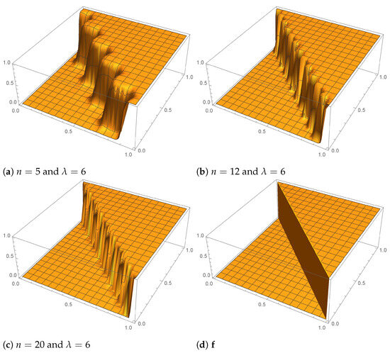
If the function $\mathbf{f}$ is considered to be a three-dimensional surface parametrized by $x_1$ and $x_2$, one can produce its three-dimensional parametric plots with the help of the Mathematica program. Similarly, we can also produce the corresponding approximations by vector-valued Shepard operators. Such parametric plots are shown in Figure 1 for the values $n=5, 12, 20$ and $\lambda =6.$ Observe that since $\mathbf{f}$ is not continuous on $\mathbf{K}$, Theorem 1 is not valid for the function $\mathbf{f}$ given by (11). Hence, this example explains why we also need the Kantorovich version of vector-valued Shepard operators.

Figure 1. Parametric plots of ${\mathbb{L}}_{n,\lambda }\left(\mathbf{f}\right)$ for the values $n=5, 12, 20$ and $\lambda =6$, where $\mathbf{f}$ is given by (11).

Example 2. 

Take $d=3$ and $m=1.$ Now define the function $\mathbf{h}$ on the set $\mathbf{K}=[0,1]$ by

$$\mathbf{h}\left(x\right)=\left(sin\left(20x\right),cos\left(20x\right),2x\right).$$

(12)

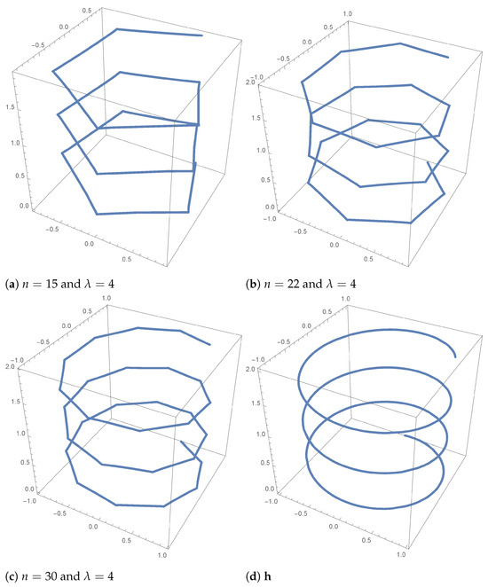
Then this function parametrized by x gives a helix curve. Since $\mathbf{h}\in C\left(\mathbf{K},{\mathbb{R}}^3\right)$, we obtain from Theorems 1 and 3 that for every $\lambda \ge 2,$

$${\mathbb{L}}_{n,\lambda }\left(\mathbf{h}\right)\rightrightarrows \mathbf{h}on[0,1]$$

and

$${\mathbb{L}}_{n,\lambda }\left(\mathbf{h}\right)\to \mathbf{h}in{L}_p\left([0,1],{\mathbb{R}}^3\right).$$

This approximation is indicated in Figure 2 for the values $n=15, 22, 30$ and $\lambda =4.$

Figure 2. Parametric plots of ${\mathbb{L}}_{n,\lambda }\left(\mathbf{h}\right)$ for the values $n=15, 22, 30$ and $\lambda =4$, where $\mathbf{h}$ is given by (12).

Finally, we discuss the regular summability methods on the $L_p$-approximation. Before giving our final application, we recall some concepts from summability theory. For a given infinite matrix $A:=\left[a_{jn}\right]$$\left(j,n\in \mathbb{N}\right)$ and a sequence $x:=\left(x_n\right)$, the A-transformed sequence of $\left(x_n\right)$ is defined by $Ax:=\left({\left(Ax\right)}_j\right)={\sum }_{n=1}^{\infty }{a}_{jn}{x}_n$ provided that the series is convergent for every $j\in \mathbb{N}$. Also, $A=\left[a_{jn}\right]$ is called regular if $limAx=L$ whenever $limx=L$ (see [21]). $A=\left[a_{jn}\right]$ is nonnegative if $a_{jn}\ge 0$ for all $j,n\in \mathbb{N}$. Now let $A=\left[a_{jn}\right]$ be a nonnegative regular summability matrix. Then, we say that a sequence $\left(x_n\right)$ is A-summable (or A-convergent) to a number L if ${lim}_{n\to \infty }{\left(Ax\right)}_j=L.$ It is also possible to give the same definition for a sequence of functions in the space $L_p\left(\mathbf{K},{\mathbb{R}}^d\right)$$\left(p\ge 1\right)$. Let $\left({\mathbf{f}}_n\right)$ be a sequence of vector-valued functions in $L_p\left(\mathbf{K},{\mathbb{R}}^d\right)$, and let $A=\left[a_{jn}\right]$ be a nonnegative regular summability method such that ${\sum }_{n=1}^{\infty }{a}_{jn}{\mathbf{f}}_n\in L_p\left(\mathbf{K},{\mathbb{R}}^d\right)$ for every $j\in \mathbb{N}$. Then, we say that $\left(f_n\right)$ is A-summable to a function $\mathbf{f}$ in $L_p\left(\mathbf{K},{\mathbb{R}}^d\right)$ if ${\sum }_{n=1}^{\infty }{a}_{jn}{\mathbf{f}}_n\to \mathbf{f}$ in $L_p\left(\mathbf{K},{\mathbb{R}}^d\right)$ as $j\to \infty$. As stated before, here we mean the componentwise $L_p$-convergence on $\mathbf{K}$.

We should note that the use of regular summability methods in the approximation theory enables us to get more powerful results than the classical ones. We will now consider an application in this direction.

Example 3. 

In this application, we modify the vector-valued Kantorovich–Shepard operators in (2) as follows:

$${\mathbb{L}}_{n,\lambda }^{*}(\mathbf{f};\mathbf{x}):=\left\{\begin{array}{cc}\mathbf{1}+\mathbf{f}\left(\mathbf{x}\right),\hfill & ifn=k^2\left(k\in \mathbb{N}\right)\hfill \\ {\mathbb{L}}_{n,\lambda }(\mathbf{f};\mathbf{x})\hfill & \mathit{otherwise},\hfill \end{array}\right.$$

(13)

where $\mathbf{1}=\left(1,1,\dots ,1\right)$. Since $\mathbf{1}+\mathbf{f}\ne \mathbf{f}$, we cannot get an $L_p$-approximation to $\mathbf{f}$ by means of the operators ${\mathbb{L}}_{n,\lambda }^{*}\left(\mathbf{f}\right)$ given by (13); that is, for every $\lambda >0$ and $i=1,2,\dots ,d,$

$${\mathbb{L}}_{n,\lambda }^{*}\left(\mathbf{f}\right)\nrightarrow \mathbf{f}in{L}_p\left(\mathbf{K},{\mathbb{R}}^d\right)asn\to \infty .$$

Now to overcome the loss of convergence, we consider the well-known Cesàro summability method $C_1:=\left[c_{jn}\right]$ (see [21] for details) given by

$$c_{jn}=\left\{\begin{array}{cc}\frac{1}{j},\hfill & ifn=1,2,\dots ,j\hfill \\ 0,\hfill & \mathit{otherwise}.\hfill \end{array}\right.$$

Let $\mathbf{f}\in L_p\left(K,{\mathbb{R}}^d\right)$$\left(p\ge 1\right)$ and $\lambda \ge m+1$ be given. Then, we observe that the arithmetic mean of ${\mathbb{L}}_{n,\lambda }^{*}\left(\mathbf{f}\right)$ is $L_p$-convergent to $\mathbf{f}$ in $L_p\left(\mathbf{K},{\mathbb{R}}^d\right)$. To see that considering the companion operator ${\tilde{L}}_{n,\lambda }^{*}$ of (13), it is enough to show that for each $i=1,2,\dots ,d$, the sequence $\left({\tilde{\mathbb{L}}}_{n,\lambda }^{*}\left(f_i\right)\right),$$i=1,2,\dots ,d,$ is $C_1$-summable (with respect to the $L_p$-norm on $\mathbf{K}$) to the function $f_i$. Indeed, by using (13) we may write that

$$\begin{array}{ccc}\hfill {∥\sum _{n=1}^{\infty }{c}_{jn}{\tilde{\mathbb{L}}}_{n,\lambda }^{*}\left(f_i\right)-f_i∥}_p& =& {∥\frac{1}{j}\sum _{n=1}^j{\tilde{\mathbb{L}}}_{n,\lambda }^{*}\left(f_i\right)-f_i∥}_p\hfill \\ & \le & \frac{1}{j}\sum _{n=1}^j{∥{\tilde{L}}_{n,\lambda }^{*}\left(f_i\right)-f_i∥}_p\hfill \\ & =& \frac{1}{j}\sum _{n=1\left(n=k^2\right)}^j{∥{\tilde{L}}_{n,\lambda }^{*}\left(f_i\right)-f_i∥}_p+\frac{1}{j}\sum _{n=1\left(n\ne k^2\right)}^j{∥{\tilde{\mathbb{L}}}_{n,\lambda }^{*}\left(f_i\right)-f_i∥}_p\hfill \\ & \le & \frac{1}{\sqrt{j}}+\frac{1}{j}\sum _{n=1}^j{∥{\tilde{\mathbb{L}}}_{n,\lambda }\left(f_i\right)-f_i∥}_p,\hfill \end{array}$$

where ${\tilde{\mathbb{L}}}_{n,\lambda }$ is the classical companion operator given by (4). Now, by taking the limit as $j\to \infty$ on both sides of the last inequality, we obtain from Theorem 2 and the regularity of the Cesàro method that for each $i=1,2,\dots ,d,$

$$\underset{j\to \infty }{lim}{∥\sum _{n=1}^{\infty }{c}_{jn}{\tilde{\mathbb{L}}}_{n,\lambda }^{*}\left(f_i\right)-f_i∥}_p=0,$$

holds, which means

$$\frac{{\mathbb{L}}_{1,\lambda }^{*}\left(\mathbf{f}\right)+{\mathbb{L}}_{2,\lambda }^{*}\left(\mathbf{f}\right)+\cdots +{\mathbb{L}}_{j,\lambda }^{*}\left(\mathbf{f}\right)}{j}\to \mathbf{f}in{L}_p\left(\mathbf{K},{\mathbb{R}}^d\right)asj\to \infty .$$

In other words, the sequence $\left({\mathbb{L}}_{n,\lambda }^{*}\left(\mathbf{f}\right)\right)$ is $C_1$-summable to $\mathbf{f}$ in $L_p\left(\mathbf{K},{\mathbb{R}}^d\right)$.

References

- Bernstein, S. Démonstration du théorème de Weierstrass fondée sur le calcul des probabilités. Commun. Kharkov Math. Soc. 1913, XIII, 1–2. [Google Scholar]
- Kantorovič, L.V. Sur certains développements suivant les polynomes de la forme de S.Bernstein, I. Comptes Rendus L’AcadéMie Des Sci. L’Urss 1930, 20, 563–568. [Google Scholar]
- Kantorovič, L.V. Sur certains développements suivant les polynomes de la forme de S.Bernstein, II. Comptes Rendus L’AcadéMie Des Sci. L’Urss 1930, 20, 595–600. [Google Scholar]
- Angeloni, L.; Vinti, G. Multidimensional sampling-Kantorovich operators in BV-spaces. Open Math. 2023, 21, 20220573. [Google Scholar] [CrossRef]
- Costarelli, D. Approximation error for neural network operators by an averaged modulus of smoothness. J. Approx. Theory 2023, 294, 105944. [Google Scholar] [CrossRef]
- Costarelli, D.; Spigler, R. Convergence of a family of neural network operators of the Kantorovich type. J. Approx. Theory 2014, 185, 80–90. [Google Scholar] [CrossRef]
- Orlova, O.; Tamberg, G. On approximation properties of generalized Kantorovich-type sampling operators. J. Approx. Theory 2016, 201, 73–86. [Google Scholar] [CrossRef]
- Duman, O.; Vecchia, B.D. Vector-Valued Shepard Processes: Approximation with Summability. Axioms 2023, 12, 1124. [Google Scholar] [CrossRef]
- Shepard, D. A two-dimensional interpolation function for irregularly-spaced data. In Proceedings of the 23rd ACM National Conference, New York, NY, USA, 27–29 August 1968; pp. 517–524. [Google Scholar]
- Della Vecchia, B. Direct and converse results by rational operators. Constr. Approx. 1996, 12, 271. [Google Scholar] [CrossRef]
- Duman, O.; Della Vecchia, B. Complex Shepard operators and their summability. Results Math. 2021, 76, 214. [Google Scholar] [CrossRef]
- Duman, O.; Della Vecchia, B. Approximation to integrable functions by modified complex Shepard operators. J. Math. Anal. Appl. 2022, 512, 126161. [Google Scholar] [CrossRef]
- Farwig, R. Rate of convergence of Shepard’s global interpolation formula. Math. Comput. 1986, 46, 577–590. [Google Scholar] [CrossRef][Green Version]
- Hermann, T. Rational interpolation of periodic functions. In Supplemento ai Rendiconti del Circolo Matematico di Palermo, Proceedings of the Second International Conference in Functional Analysis and Approximation Theory, Acquafredda di Maratea, Italy, 14–19 September 1992; Circolo Matematico di Palermo: Palermo, Italy, 1993; Series 2; Volume 33, pp. 337–344. [Google Scholar]
- Zhou, X. The saturation class of Shepard operators. Acta Math. Hung. 1998, 80, 293–310. [Google Scholar] [CrossRef]
- Dell’Accio, F.; Di Tommaso, F. Complete Hermite–Birkhoff interpolation on scattered data by combined Shepard operators. J. Comput. Appl. Math. 2016, 300, 192–206. [Google Scholar] [CrossRef]
- Dell’Accio, F.; Di Tommaso, F. On the hexagonal Shepard method. Appl. Numer. Math. 2020, 150, 51–64. [Google Scholar] [CrossRef]
- Dell’Accio, F.; Di Tommaso, F.; Hormann, K. On the approximation order of triangular Shepard interpolation. IMA J. Numer. Anal. 2016, 36, 359–379. [Google Scholar] [CrossRef]
- Mikusiński, J. The Bochner Integral; Lehrbücher und Monographien aus dem Gebiete der Exakten Wissenschaften, Mathematische Reihe; Birkhäuser Verlag: Basel, Switzerland; Stuttgart, Germany, 1978; pp. xii+233. [Google Scholar] [CrossRef]
- Zygmund, A. Trigonometric Series, 3rd ed.; Cambridge Mathematical Library, Cambridge University Press: Cambridge, UK, 2003. [Google Scholar]
- Boos, J.; Cass, P. Classical and Modern Methods in Summability; Oxford Mathematical Monographs, Oxford University Press: Oxford, UK, 2000; p. 600. [Google Scholar]
Disclaimer/Publisher’s Note: The statements, opinions and data contained in all publications are solely those of the individual author(s) and contributor(s) and not of MDPI and/or the editor(s). MDPI and/or the editor(s) disclaim responsibility for any injury to people or property resulting from any ideas, methods, instructions or products referred to in the content. |
© 2024 by the authors. Licensee MDPI, Basel, Switzerland. This article is an open access article distributed under the terms and conditions of the Creative Commons Attribution (CC BY) license (https://creativecommons.org/licenses/by/4.0/).