Comparing the Performance of Two Butcher-Based Block Hybrid Algorithms for the Solution of Initial Value Problems

Abstract

In this paper, we compare the performances of two Butcher-based block hybrid methods for the numerical integration of initial value problems. We compare the condition numbers of the linear system of equations arising from both methods and the absolute errors of the solution obtained. The results of the numerical experiments illustrate that the better conditioned method outperformed its less conditioned counterpart based on the absolute errors. In addition, after applying our method on some examples, it was discovered that the absolute errors in this work were better than those of a recent study in the literature. Hence, we recommend this method for the numerical solution of stiff and non-stiff initial value problems.

1. Introduction

Differential equations play crucial roles in ecology, modeling, chemical kinetics, engineering, population dynamics and medicine. Some of them do not have exact or closed-form solutions and it is imperative to find new numerical methods on the one hand or improve upon already existing methods on the other. More precisely, this paper considers finding numerical approximations to first-order initial valued systems of ordinary differential equations of the form;

$$y^{\prime }\left(x\right)=f(x,y),x\in \mathbb{R},$$

(1)

on the interval $[a,b]$ subject to the initial condition $y\left(a\right)=y_0$, with $f:{\mathbb{R}}^r\to {\mathbb{R}}^r,r\in \mathbb{N}-\left\{0\right\}$. One of the numerical methods for solving systems of differential equations is linear multi-step methods which though powerful but most times suffers the disadvantage that matrices arising from its use are often ill-conditioned according to Shampine [1]. As a result of this and according to Trefethen and Bau [2] p. 95, if a system is ill-conditioned, then one may lose the logarithm to base 10 of the condition number of the matrix’s significant digits. However, there is paucity of literature on this topic of overcoming ill-conditioning as it relates to linear multi-step methods, though the subject of ill-conditioning, as it pertains to linear systems of equations, is well-studied.

In addition to this, block hybrid methods which incorporate interpolating and collocating at both grid and off grid points multiplies the size of the linear system to be solved, thereby increasing the propensity of the linear multi-step-based method to ill-conditioning. While Runge–Kutta methods, on the other hand, suffer the inherent problem of requiring much more cputime time than their linear multi-step methods counterpart. Hence, a linear multi-step method that is computationally cheap, stable and well-conditioned is often sought. That is why, in this study, we improve upon the two-step Butcher’s block hybrid method which is numerically better conditioned with the exception of outperforming those in the literature for non-linear systems of differential equations.

The two-step Butcher’s hybrid scheme has been derived by several authors [3,4,5,6,7,8] using different off-grid points. The two-step Butcher’s block hybrid method is a linear multi-step of order five for the numerical solution of one- and high-dimensional systems of ordinary differential equations which is the crux of the matter in this article. In an earlier work, we showed that, for one-dimensional stiff and non-stiff, linear and nonlinear differential equations, the performance of the Butcher-based block hybrid method obtained at the points $\{1,\frac{3}{2},\frac{7}{4},2\}$ with those obtained at $\{1,\frac{3}{2},2,\frac{5}{2}\}$ were at par, though the latter was better conditioned than the former. In order to avoid abuse of notation, for the purpose of this study, we will refer to $y_{n+\frac{7}{4}}$ as the block hybrid method obtained at the following combination of grid and off-grid points: $\{1,\frac{3}{2},\frac{7}{4},2\}$ and $y_{n+\frac{5}{2}}$ the block hybrid method obtained at the latter points $\{1,\frac{3}{2},2,\frac{5}{2}\}$ in line with [7].

In fact, this work is an extension of the works of Akinola et al. [7], where both methods were shown to be of order five and convergent. Nevertheless, we did not compare their regions of absolute stability nor their error constants because the goal in that study was to provide a brief solution to Shampine’s [1] claim about the ill-conditioning of matrices obtained from linear multi-step methods (see also [9,10,11,12,13,14,15,16]) and solving first order differential equations. No Jacobian was presented in that paper nor any proof of the non-singularity of the corresponding Jacobians, neither did we provide any algorithms.

In [6] we gave a proof of the non-singularity of the D matrix used when deriving the two-step Butcher’s hybrid scheme for the solution of initial value problems. However, the test problems were one-dimensional. In addition to our discussion in the second to the last paragraph above, the focus in [7] was to discuss with numerical examples how ill-conditioning arising from using linear multi-step methods in approximating the solution of initial value problems could be reduced, albeit for one-dimensional ODEs, which is also an improvement from the works in [8]. Similarly, Adee and Atabo [17] presented a two point linear multi-step method for solving similar problems as the ones considered in [7] and the present work, except that their method is non starting and they used a fourth order Runge–Kutta method in obtaining the starting values. In this work, our method is self-starting and does not rely on other methods to start (see also [18,19,20,21,22,23,24,25].)

In this work, we extend the idea in [7] to numerical examples of two, three, four and six-dimensional systems of differential equations to confirm the earlier claim that $y_{n+\frac{5}{2}}$ is better well-conditioned than those of $y_{n+\frac{7}{4}}$. We compared their respective absolute errors and cputime to see which performs better between the two. The plan of this study is as follows: in Section 1, we give an overview of the content of this article, which is followed in Section 2, where we present the continuous form of the block hybrid method and state important results and in Section 3 we examine the convergence and give the appropriate algorithms of the methods. Finally, we conclude by presenting the results of the numerical experiments which validate and confirm the theory in Section 4.

2. Methodology

The emphasis in this section is two folds: we re-present the continuous formulation from which the two block hybrid methods $y_{n+\frac{7}{4}}$ and $y_{n+\frac{5}{2}}$ are derived at various grid and off grid points. Secondly, we show that the respective Jacobians (to be defined shortly) are non-singular at the root.

Derivation of Multi-Step Collocation Methods

Following in the footsteps of Onumanyi et al. [26], we present the re–derivation of our method, where a 2-step multi-step method having m collocation points is

$${\displaystyle y\left(x\right)=\sum _{j=0}^{t-1}{\alpha }_j\left(x\right)y\left(x_{n+j}\right)+h\sum _{j=0}^{m-1}{\beta }_j\left(x\right)f(x_j,y\left(x_j\right)),}$$

(2)

where ${\alpha }_j\left(x\right)$ and ${\beta }_j\left(x\right)$

$${\displaystyle {\alpha }_j\left(x\right)=\sum _{j=0}^{t+m-1}{\alpha }_{j,i+1}{x}^i,h{\beta }_j\left(x\right)=h\sum _{j=0}^{t+m-1}{\beta }_{j,i+1}{x}^i,}$$

(3)

are the continuous coefficients for $j=0,1,\cdots ,t-1$. The $t(0<t\le k)$ in (2) are interpolation points taken from $\{x_0,x_1,\cdots ,x_{n+k}\}$ and $x_j$ for $j=0,1,2,\cdots ,m-1$ are the m collocation points belonging to $\{x_0,x_1,\cdots ,x_{n+k}\}$. To obtain ${\alpha }_j\left(x\right),{\beta }_j\left(x\right)$, Onumanyi [26] used at a matrix equation of the form $DC=I$, where I is an identity matrix of size $(t+m)$, and D and C are matrices defined by

$$D=\left[\begin{array}{cccccc}1& x_n& x_n^2& x_n^3& \cdots & {\displaystyle x_n^{t+m-1}}\\ \\ 1& x_{n+1}& x_{n+1}^2& x_{n+1}^3& \cdots & {\displaystyle x_{n+1}^{t+m-1}}\\ \\ ⋮& ⋮& ⋮& ⋮& \cdots & ⋮\\ \\ 1& x_{n+t-1}& x_{n+t-1}^2& x_{n+t-1}^3& \cdots & {\displaystyle x_{n+t-1}^{t+m-1}}\\ \\ 0& 1& 2x_n& 3x_n^2& \cdots & {\displaystyle (t+m-1)x_n^{t+m-1}}\\ \\ ⋮& ⋮& ⋮& ⋮& \cdots & ⋮\\ \\ 0& 1& 2x_{n+\delta }& 3x_{n+\delta }^2& \cdots & {\displaystyle (t+m-1)x_{n+\delta }^{t+m-1}}\end{array}\right].$$

(4)

The matrix in (4) is the collocation matrix of size $(t+m)\times (t+m)$ as C. The matrix C whose first row gives the continuous coefficients is defined as

$$C=\left[\begin{array}{cccccc}{\alpha }_{0,1}& {\alpha }_{1,1}& \cdots {\alpha }_{t-1,1}& h{\beta }_{0,1}& \cdots & h{\beta }_{m-1,1}\\ \\ {\alpha }_{0,2}& {\alpha }_{1,2}& \cdots {\alpha }_{t-1,2}& h{\beta }_{0,2}& \cdots & h{\beta }_{m-1,2}\\ \\ ⋮& ⋮& ⋮& ⋮& ⋮& ⋮\\ \\ {\alpha }_{0,t+m}& {\alpha }_{1,t+m}& \cdots {\alpha }_{t-1,t+m}& h{\beta }_{0,t+m}& \cdots & h{\beta }_{m-1,t+m}\end{array}\right].$$

(5)

Let $y_n$ be an approximation to the theoretical solution at $x_n$, that is, $y_n\approx y\left(x_n\right)$ and let $f_n=f(x_n,y_n)$, $y_{n+j}=y\left(x_{n+j}\right)=y(x_n+jh)$ and $f_{n+j}=f(x_{n+j},y_{n+j})=f(x_n+jh,y(x_n+jh)),$ for $j\in \{1,\frac{3}{2},2\},x_i=x_0+ih,i=0,1,2,\cdots ,N-1,h=\frac{b-a}{N}.$

We substituted $t=2$, $m=4$ and $\delta \in \{1,3/2,2\}$ into (2) to obtain the continuous formulation of the two-step Butcher’s block hybrid method:

$$y\left(x\right)={\alpha }_0\left(x\right)y_n+{\alpha }_1\left(x\right)y_{n+1}+h\left[{\beta }_0\left(x\right)f_n+{\beta }_1\left(x\right)f_{n+1}+{\beta }_{\frac{3}{2}}\left(x\right)f_{n+\frac{3}{2}}+{\beta }_2\left(x\right)f_{n+2}\right],$$

(6)

and D from (4) reduces to

$$D=\left[\begin{array}{cccccc}1& x_n& x_n^2& x_n^3& x_n^4& x_n^5\\ \\ 1& x_{n+1}& x_{n+1}^2& x_{n+1}^3& x_{n+1}^4& x_{n+1}^5\\ \\ 0& 1& 2x_n& 3x_n^2& 4x_n^3& 5x_n^4\\ \\ 0& 1& 2x_{n+1}& 3x_{n+1}^2& 4x_{n+1}^3& 5x_{n+1}^4\\ \\ 0& 1& 2x_{n+2}& 3x_{n+2}^2& 4x_{n+2}^3& 5x_{n+2}^4\\ \\ 0& 1& 2x_{n+\frac{3}{2}}& 3x_{n+\frac{3}{2}}^2& 4x_{n+\frac{3}{2}}^3& 5x_{n+\frac{3}{2}}^4\end{array}\right].$$

(7)

Replacing $x_n=x_{n+1}-h$, $x_{n+\frac{3}{2}}=x_{n+1}+\frac{h}{2}$ and $x_{n+2}=x_{n+1}+h$, the determinant of D is

$$detD=\frac{93h^{11}}{4}.$$

(8)

The following continuous scheme was discussed in [6] with $\mu =x_{n+1}-x$:

$$\begin{array}{cc}\hfill y\left(x\right)& =\left[\frac{-24{\mu }^5-15h{\mu }^4+40h^2{\mu }^3+30h^3{\mu }^2}{31h^5}\right]y_n+\left[\frac{24{\mu }^5+15h{\mu }^4-40h^2{\mu }^3-30h^3{\mu }^2+31h^5}{31h^5}\right]y_{n+1}\hfill \\ \\ \hfill & +\left[\frac{-96{\mu }^5-91h{\mu }^4+98h^2{\mu }^3+89h^3{\mu }^2}{372h^4}\right]f_n+\left[\frac{-28{\mu }^5-2h{\mu }^4+57h^2{\mu }^3+4h^3{\mu }^2-31h^4\mu }{31h^4}\right]f_{n+1}\hfill \\ \\ \hfill & +\left[\frac{48{\mu }^5-32h{\mu }^4-80h^2{\mu }^3+64h^3{\mu }^2}{93h^4}\right]f_{n+\frac{3}{2}}+\left[\frac{-16{\mu }^5+21h{\mu }^4+6h^2{\mu }^3-11h^3{\mu }^2}{124h^4}\right]f_{n+2}.\hfill \end{array}$$

(9)

Differentiate the continuous formulation with respect to $\mu$, evaluating the derivative at $\mu =-\frac{3h}{4}$ and making $y_{n+1}$ the subject results in (10). The differentiation is important in this context because we want to obtain a square system of four equations in four unknowns. In addition to this, without the differentiation and subsequent substitution, an under–determined system of three equations in four unknowns will suffice and this has been shown in [7] not to give accurate approximations to the exact solution. Moreover, it allows us to add an extra function evaluation point $f_{n+\frac{7}{4}}$, thereby improving the accuracy. In the same vein, evaluating (9) at the following points $\mu =\{-\frac{3h}{4},-\frac{h}{2},-h\}$. That is, when $\mu =-\frac{3h}{4}$, using $\mu =x_{n+1}-x$, $-\frac{3h}{4}=x_{n+1}-x$, $x=x_{n+1}+\frac{3h}{4}=x_{n+\frac{7}{4}}$. Hence,

$$y\left(x\right)=y(x_{n+\frac{7}{4}})=y_{n+\frac{7}{4}}.$$

When $\mu =-\frac{h}{2}$, $-\frac{h}{2}=x_{n+1}-x$, $x=x_{n+1}+\frac{h}{2}=x_{n+\frac{3}{2}}$. Thus,

$$y\left(x\right)=y(x_{n+\frac{3}{2}})=y_{n+\frac{3}{2}}.$$

Finally, when $\mu =-h$, $-h=x_{n+1}-x$, $x=x_{n+1}+h=x_{n+2}$. Thus,

$$y\left(x\right)=y\left(x_{n+2}\right)=y_{n+2}.$$

Therefore, we have explained the link between $\mu$ and the left-hand sides. Hence, after the same substitutions have been made to the right-hand sides, we obtained the remaining schemes (11)–(13):

$$\begin{array}{ccc}\hfill y_{n+1}& =& y_n+\frac{h}{630}\left[-179f_n-1169f_{n+1}+2156f_{n+\frac{3}{2}}-1984f_{n+\frac{7}{4}}+546f_{n+2}\right],\hfill \end{array}$$

(10)

$$\begin{array}{ccc}\hfill y_{n+\frac{3}{2}}& =& \frac{37}{496}{y}_n+\frac{459}{496}{y}_{n+1}+\frac{h}{1984}\left[39f_n+648f_{n+1}+480f_{n+\frac{3}{2}}-27f_{n+2}\right],\hfill \end{array}$$

(11)

$$\begin{array}{ccc}\hfill y_{n+\frac{7}{4}}& =& \frac{243}{7936}{y}_n+\frac{7693}{7936}{y}_{n+1}+\frac{h}{31744}\left[231f_n+7644f_{n+1}+16464f_{n+\frac{3}{2}}+441f_{n+2}\right],\hfill \end{array}$$

(12)

$$\begin{array}{ccc}\hfill y_{n+2}& =& -\frac{1}{31}{y}_n+\frac{32}{31}{y}_{n+1}+\frac{h}{93}\left[-f_n+12f_{n+1}+64f_{n+\frac{3}{2}}+15f_{n+2}\right].\hfill \end{array}$$

(13)

The above schemes (10)–(13) is what makes up the block hybrid method which we denote by $y_{n+\frac{7}{4}}$ for ease of reference. It can be expressed as the following nonlinear system:

$$\begin{array}{c}\hfill y_{n+1}-y_n-\frac{h}{630}\left[-179f_n-1169f_{n+1}+2156f_{n+\frac{3}{2}}-1984f_{n+\frac{7}{4}}+546f_{n+2}\right]=0,\\ \hfill y_{n+\frac{3}{2}}-\frac{37}{496}{y}_n-\frac{459}{496}{y}_{n+1}-\frac{h}{1984}\left[39f_n+648f_{n+1}+480f_{n+\frac{3}{2}}-27f_{n+2}\right]=0,\\ \hfill y_{n+\frac{7}{4}}-\frac{243}{7936}{y}_n-\frac{7693}{7936}{y}_{n+1}-\frac{h}{31744}\left[231f_n+7644f_{n+1}+16464f_{n+\frac{3}{2}}+441f_{n+2}\right]=0,\\ \hfill y_{n+2}+\frac{1}{31}{y}_n-\frac{32}{31}{y}_{n+1}-\frac{h}{93}\left[-f_n+12f_{n+1}+64f_{n+\frac{3}{2}}+15f_{n+2}\right]=0.\end{array}$$

For $r=1$, the Jacobian of the above nonlinear system is

$$J_7=\left[\begin{array}{cccc}\frac{167h}{90}\frac{\partial f_{n+1}}{\partial y_{n+1}}-1& -\frac{154h}{45}\frac{\partial f_{n+\frac{3}{2}}}{\partial y_{n+\frac{3}{2}}}& \frac{992h}{315}\frac{\partial f_{n+\frac{7}{4}}}{\partial y_{n+\frac{7}{4}}}& -\frac{13h}{15}\frac{\partial f_{n+2}}{\partial y_{n+2}}\\ \\ -\frac{81h}{248}\frac{\partial f_{n+1}}{\partial y_{n+1}}-\frac{459}{496}& 1-\frac{15h}{62}\frac{\partial f_{n+\frac{3}{2}}}{\partial y_{n+\frac{3}{2}}}& 0& \frac{27h}{1984}\frac{\partial f_{n+2}}{\partial y_{n+2}}\\ \\ -\frac{1911h}{7936}\frac{\partial f_{n+1}}{\partial y_{n+1}}-\frac{7693}{7936}& -\frac{1029h}{1984}\frac{\partial f_{n+\frac{3}{2}}}{\partial y_{n+\frac{3}{2}}}& 1& -\frac{441h}{31744}\frac{\partial f_{n+2}}{\partial y_{n+2}}\\ \\ -\frac{4h}{31}\frac{\partial f_{n+1}}{\partial y_{n+1}}-\frac{32}{31}& -\frac{64h}{93}\frac{\partial f_{n+\frac{3}{2}}}{\partial y_{n+\frac{3}{2}}}& 0& 1-\frac{5h}{31}\frac{\partial f_{n+2}}{\partial y_{n+2}}\end{array}\right].$$

(14)

Lemma 1. 

The Jacobian $J_7$ in (14) is nonsingular at the root.

Proof. 

After carrying out elementary row operations, we obtained

$$\sim \left[\begin{array}{cccc}1& \frac{120\frac{\partial f_{n+\frac{3}{2}}}{\partial y_{n+\frac{3}{2}}}h-496}{162h\frac{\partial f_{n+1}}{\partial y_{n+1}}+459}& 0& -\frac{h\frac{\partial f_{n+2}}{\partial y_{n+2}}}{24h\frac{\partial f_{n+1}}{\partial y_{n+1}}+68}\\ \\ 0& 1& 0& \frac{27h^2\frac{\partial f_{n+1}}{\partial y_{n+1}}\frac{\partial f_{n+2}}{\partial y_{n+2}}+\left(81\frac{\partial f_{n+2}}{\partial y_{n+2}}-162\frac{\partial f_{n+1}}{\partial y_{n+1}}\right)h-459}{96h^2\frac{\partial f_{n+1}}{\partial y_{n+1}}\frac{\partial f_{n+\frac{3}{2}}}{\partial y_{n+\frac{3}{2}}}+\left(192\frac{\partial f_{n+\frac{3}{2}}}{\partial y_{n+\frac{3}{2}}}+64\frac{\partial f_{n+1}}{\partial y_{n+1}}\right)h+512}\\ \\ 0& 0& 1& \nu \\ \\ 0& 0& 0& 1\end{array}\right],$$

where

$$\begin{array}{cc}\hfill \nu & =\frac{441h^3\frac{\partial f_{n+1}}{\partial y_{n+1}}\frac{\partial f_{n+\frac{3}{2}}}{\partial y_{n+\frac{3}{2}}}\frac{\partial f_{n+2}}{\partial y_{n+2}}+\left[\left(1029\frac{\partial f_{n+\frac{3}{2}}}{\partial y_{n+\frac{3}{2}}}+1176\frac{\partial f_{n+1}}{\partial y_{n+1}}\right)\frac{\partial f_{n+2}}{\partial y_{n+2}}-3528\frac{\partial f_{n+1}}{\partial y_{n+1}}\frac{\partial f_{n+\frac{3}{2}}}{\partial y_{n+\frac{3}{2}}}\right]h^2}{6144h^2\frac{\partial f_{n+1}}{\partial y_{n+1}}\frac{\partial f_{n+\frac{3}{2}}}{\partial y_{n+\frac{3}{2}}}+\left(12288\frac{\partial f_{n+\frac{3}{2}}}{\partial y_{n+\frac{3}{2}}}+4096\frac{\partial f_{n+1}}{\partial y_{n+1}}\right)h+32768}\hfill \\ \hfill & +\frac{\left(4508\frac{\partial f_{n+2}}{\partial y_{n+2}}-7791\frac{\partial f_{n+\frac{3}{2}}}{\partial y_{n+\frac{3}{2}}}-7644\frac{\partial f_{n+1}}{\partial y_{n+1}}\right)h-30772}{6144h^2\frac{\partial f_{n+1}}{\partial y_{n+1}}\frac{\partial f_{n+\frac{3}{2}}}{\partial y_{n+\frac{3}{2}}}+\left(12288\frac{\partial f_{n+\frac{3}{2}}}{\partial y_{n+\frac{3}{2}}}+4096\frac{\partial f_{n+1}}{\partial y_{n+1}}\right)h+32768}.\hfill \end{array}$$

Its determinant which is the product of the diagonal elements is one. Hence, $J_7$ is nonsingular.    □

An alternative proof of the above result using Keller’s ABCD Lemma [27] is given below, but before then, we give a brief synopsis on the ABCD Lemma. The implicit determinant method of Spence and Poulton [28] is an application of Newton’s method in finding the zeros of certain bordered matrices arising from finding a photonic band structure in periodic materials such as photonic crystals. Nevertheless, at the heart of the implicit determinant method is Keller’s ABCD Lemma [27], whereby a partitioned matrix is shown to be nonsingular under certain conditions. The “ABCD” Lemma has been used in [29,30,31] in different ways to show that certain parameter-dependent matrices are nonsingular and Newton’s method is applied accordingly. The Lemma, as the name implies, relies on splitting a matrix into its partitioned ABCD components, and after certain conditions which must have been satisfied, the matrix under consideration is described as non-singular or as maybe not the case. These references and others form our motivation for using the ABCD Lemma to show that the Jacobians in this work are non-singular, as shown below.

We state without proof the one-dimensional version of Keller’s [27] ABCD Lemma. The aim is to use it in proving the non-singularity of the one-dimensional version of $J_7$.

Lemma 2. 

“ABCD” Lemma.

Let $\mathbf{A}\in {\mathbb{R}}^{n\times n}$, $\mathbf{b},\mathbf{c}\in {\mathbb{R}}^n$, $d\in \mathbb{R}$ and

$$J_7=\left[\begin{array}{cc}\mathbf{A}& \mathbf{b}\\ {\mathbf{c}}^T& d\end{array}\right]\in {\mathbb{R}}^{(n+1)\times (n+1)}.$$

(15)

Assume that $\mathbf{A}$ is non-singular; then, $J_7$ has the following decomposition:

$$\left[\begin{array}{cc}\mathbf{A}& \mathbf{b}\\ {\mathbf{c}}^T& d\end{array}\right]=\left[\begin{array}{cc}\mathbf{I}& \mathbf{0}\\ {\mathbf{c}}^T{\mathbf{A}}^{-1}& 1\end{array}\right]\left[\begin{array}{cc}\mathbf{A}& \mathbf{b}\\ {\mathbf{0}}^T& d-{\mathbf{c}}^T{\mathbf{A}}^{-1}\mathbf{b}\end{array}\right].$$

(16)

The matrix $J_7$ is non-singular if $d-{\mathbf{c}}^T{\mathbf{A}}^{-1}\mathbf{b}\ne 0$.

Proof. 

Following [27], we split $J_7$; thus,

$$\mathbf{A}=\left[\begin{array}{ccc}\frac{167}{90}\frac{\partial f_{n+1}}{\partial y_{n+1}}h-1& -\frac{154}{45}\frac{\partial f_{n+\frac{3}{2}}}{\partial y_{n+\frac{3}{2}}}h& \frac{992}{315}\frac{\partial f_{n+\frac{7}{4}}}{\partial y_{n+\frac{7}{4}}}h\\ \\ -\frac{81}{248}\frac{\partial f_{n+1}}{\partial y_{n+1}}h-\frac{459}{496}& 1-\frac{15}{62}\frac{\partial f_{n+\frac{3}{2}}}{\partial y_{n+\frac{3}{2}}}h& 0\\ \\ -\frac{1911}{7936}\frac{\partial f_{n+1}}{\partial y_{n+1}}h-\frac{7693}{7936}& -\frac{1029}{1984}\frac{\partial f_{n+\frac{3}{2}}}{\partial y_{n+\frac{3}{2}}}h& 1\end{array}\right]\in {\mathbb{R}}^{3\times 3},$$

$$\mathbf{b}=\left[\begin{array}{c}-\frac{13}{15}\frac{\partial f_{n+2}}{\partial y_{n+2}}h\\ \\ \frac{27}{1984}\frac{\partial f_{n+2}}{\partial y_{n+2}}h\\ \\ -\frac{441}{31744}\frac{\partial f_{n+2}}{\partial y_{n+2}}h\end{array}\right]\in {\mathbb{R}}^{3\times 1},$$

$${\mathbf{c}}^T=\left[\begin{array}{ccc}-\frac{4}{31}\frac{\partial f_{n+1}}{\partial y_{n+1}}h-\frac{32}{31}& -\frac{64}{93}\frac{\partial f_{n+\frac{3}{2}}}{\partial y_{n+\frac{3}{2}}}h& 0\end{array}\right]\in {\mathbb{R}}^{1\times 3},\mathrm{and}d=1-\frac{5}{31}\frac{\partial f_{n+2}}{\partial y_{n+2}}h\in \mathbb{R}.$$

Before we apply the above Lemma, we need to show that $\mathbf{A}$ is non-singular. Hence, using elementary row operations, it reduces to

$$\sim \left[\begin{array}{ccc}1& \frac{120\frac{\partial f_{n+\frac{3}{2}}}{\partial y_{n+\frac{3}{2}}}h-496}{162\frac{\partial f_{n+1}}{\partial y_{n+1}}h+459}& 0\\ \\ 0& 1& -\frac{10368\frac{\partial f_{n+1}}{\partial y_{n+1}}h+29376}{3528\frac{\partial f_{n+1}}{\partial y_{n+1}}\frac{\partial f_{n+\frac{3}{2}}}{\partial y_{n+\frac{3}{2}}}{h}^2+\left(7791\frac{\partial f_{n+\frac{3}{2}}}{\partial y_{n+\frac{3}{2}}}+7644\frac{\partial f_{n+1}}{\partial y_{n+1}}\right)h+30772}\\ \\ 0& 0& 1\end{array}\right].$$

Since the pivots are three, A is indeed nonsingular.

Now, we give a condition under which $d-{\mathbf{c}}^T{\mathbf{A}}^{-1}\mathbf{b}\ne 0$. The scalar $d-{\mathbf{c}}^T{\mathbf{A}}^{-1}\mathbf{b}$ will be non-zero if and only if the terms in h in the numerator do not add up to $-1440$ as shown below:

$$\begin{array}{cc}\hfill d-{\mathbf{c}}^T{\mathbf{A}}^{-1}\mathbf{b}& =-\frac{63\frac{\partial f_{n+1}}{\partial y_{n+1}}\frac{\partial f_{n+\frac{3}{2}}}{\partial y_{n+\frac{3}{2}}}\frac{\partial f_{n+\frac{7}{4}}}{\partial y_{n+\frac{7}{4}}}\frac{\partial f_{n+2}}{\partial y_{n+2}}{h}^4+\left(\left(\left(147\frac{\partial f_{n+\frac{3}{2}}}{\partial y_{n+\frac{3}{2}}}+168\frac{\partial f_{n+1}}{\partial y_{n+1}}\right)\frac{\partial f_{n+\frac{7}{4}}}{\partial y_{n+\frac{7}{4}}}-156\frac{\partial f_{n+1}}{\partial y_{n+1}}\frac{\partial f_{n+\frac{3}{2}}}{\partial y_{n+\frac{3}{2}}}\right)\frac{\partial f_{n+2}}{\partial y_{n+2}}-504\frac{\partial f_{n+1}}{\partial y_{n+1}}\frac{\partial f_{n+\frac{3}{2}}}{\partial y_{n+\frac{3}{2}}}\frac{\partial f_{n+\frac{7}{4}}}{\partial y_{n+\frac{7}{4}}}\right)h^3}{504\frac{\partial f_{n+1}}{\partial y_{n+1}}\frac{\partial f_{n+\frac{3}{2}}}{\partial y_{n+\frac{3}{2}}}\frac{\partial f_{n+\frac{7}{4}}}{\partial y_{n+\frac{7}{4}}}{h}^3+\left(\left(1113\frac{\partial f_{n+\frac{3}{2}}}{\partial y_{n+\frac{3}{2}}}+1092\frac{\partial f_{n+1}}{\partial y_{n+1}}\right)\frac{\partial f_{n+\frac{7}{4}}}{\partial y_{n+\frac{7}{4}}}-2256\frac{\partial f_{n+1}}{\partial y_{n+1}}\frac{\partial f_{n+\frac{3}{2}}}{\partial y_{n+\frac{3}{2}}}\right)h^2+\left(4396\frac{\partial f_{n+\frac{7}{4}}}{\partial y_{n+\frac{7}{4}}}-4212\frac{\partial f_{n+\frac{3}{2}}}{\partial y_{n+\frac{3}{2}}}+2672\frac{\partial f_{n+1}}{\partial y_{n+1}}\right)h-1440}\hfill \\ \hfill & -\frac{\left(\left(644\frac{\partial f_{n+\frac{7}{4}}}{\partial y_{n+\frac{7}{4}}}-252\frac{\partial f_{n+\frac{3}{2}}}{\partial y_{n+\frac{3}{2}}}+592\frac{\partial f_{n+1}}{\partial y_{n+1}}\right)\frac{\partial f_{n+2}}{\partial y_{n+2}}+\left(-1113\frac{\partial f_{n+\frac{3}{2}}}{\partial y_{n+\frac{3}{2}}}-1092\frac{\partial f_{n+1}}{\partial y_{n+1}}\right)\frac{\partial f_{n+\frac{7}{4}}}{\partial y_{n+\frac{7}{4}}}+2256\frac{\partial f_{n+1}}{\partial y_{n+1}}\frac{\partial f_{n+\frac{3}{2}}}{\partial y_{n+\frac{3}{2}}}\right)h^2}{504\frac{\partial f_{n+1}}{\partial y_{n+1}}\frac{\partial f_{n+\frac{3}{2}}}{\partial y_{n+\frac{3}{2}}}\frac{\partial f_{n+\frac{7}{4}}}{\partial y_{n+\frac{7}{4}}}{h}^3+\left(\left(1113\frac{\partial f_{n+\frac{3}{2}}}{\partial y_{n+\frac{3}{2}}}+1092\frac{\partial f_{n+1}}{\partial y_{n+1}}\right)\frac{\partial f_{n+\frac{7}{4}}}{\partial y_{n+\frac{7}{4}}}-2256\frac{\partial f_{n+1}}{\partial y_{n+1}}\frac{\partial f_{n+\frac{3}{2}}}{\partial y_{n+\frac{3}{2}}}\right)h^2+\left(4396\frac{\partial f_{n+\frac{7}{4}}}{\partial y_{n+\frac{7}{4}}}-4212\frac{\partial f_{n+\frac{3}{2}}}{\partial y_{n+\frac{3}{2}}}+2672\frac{\partial f_{n+1}}{\partial y_{n+1}}\right)h-1440}\hfill \\ \hfill & -\frac{\left(1056\frac{\partial f_{n+2}}{\partial y_{n+2}}-4396\frac{\partial f_{n+\frac{7}{4}}}{\partial y_{n+\frac{7}{4}}}+4212\frac{\partial f_{n+\frac{3}{2}}}{\partial y_{n+\frac{3}{2}}}-2672\frac{\partial f_{n+1}}{\partial y_{n+1}}\right)h+1440}{504\frac{\partial f_{n+1}}{\partial y_{n+1}}\frac{\partial f_{n+\frac{3}{2}}}{\partial y_{n+\frac{3}{2}}}\frac{\partial f_{n+\frac{7}{4}}}{\partial y_{n+\frac{7}{4}}}{h}^3+\left(\left(1113\frac{\partial f_{n+\frac{3}{2}}}{\partial y_{n+\frac{3}{2}}}+1092\frac{\partial f_{n+1}}{\partial y_{n+1}}\right)\frac{\partial f_{n+\frac{7}{4}}}{\partial y_{n+\frac{7}{4}}}-2256\frac{\partial f_{n+1}}{\partial y_{n+1}}\frac{\partial f_{n+\frac{3}{2}}}{\partial y_{n+\frac{3}{2}}}\right)h^2+\left(4396\frac{\partial f_{n+\frac{7}{4}}}{\partial y_{n+\frac{7}{4}}}-4212\frac{\partial f_{n+\frac{3}{2}}}{\partial y_{n+\frac{3}{2}}}+2672\frac{\partial f_{n+1}}{\partial y_{n+1}}\right)h-1440}.\hfill \end{array}$$

Alternatively, as h tends to zero, all terms in h tends to zero and the above expression becomes $d-{\mathbf{c}}^T{\mathbf{A}}^{-1}\mathbf{b}=-1$. Hence, the one-dimensional Jacobian matrix $J_7$ is non-singular using the ABCD Lemma.    □

For higher-dimensional systems, i.e., $r\ge 2$ of differential equations, the analogous Jacobian is

$$J_7=\left[\begin{array}{cccc}\frac{167h}{90}\frac{\partial f_{n+1}}{\partial y_{n+1}}-\mathbf{I}& -\frac{154h}{45}\frac{\partial f_{n+\frac{3}{2}}}{\partial y_{n+\frac{3}{2}}}& \frac{992h}{315}\frac{\partial f_{n+\frac{7}{4}}}{\partial y_{n+\frac{7}{4}}}& -\frac{13h}{15}\frac{\partial f_{n+2}}{\partial y_{n+2}}\\ \\ -\frac{81h}{248}\frac{\partial f_{n+1}}{\partial y_{n+1}}-\frac{459}{496}\mathbf{I}& \mathbf{I}-\frac{15h}{62}\frac{\partial f_{n+\frac{3}{2}}}{\partial y_{n+\frac{3}{2}}}& \mathbf{O}& \frac{27h}{1984}\frac{\partial f_{n+2}}{\partial y_{n+2}}\\ \\ -\frac{1911h}{7936}\frac{\partial f_{n+1}}{\partial y_{n+1}}-\frac{7693}{7936}\mathbf{I}& -\frac{1029h}{1984}\frac{\partial f_{n+\frac{3}{2}}}{\partial y_{n+\frac{3}{2}}}& \mathbf{I}& -\frac{441h}{31744}\frac{\partial f_{n+2}}{\partial y_{n+2}}\\ \\ -\frac{4h}{31}\frac{\partial f_{n+1}}{\partial y_{n+1}}-\frac{32}{31}\mathbf{I}& -\frac{64h}{93}\frac{\partial f_{n+\frac{3}{2}}}{\partial y_{n+\frac{3}{2}}}& \mathbf{O}& \mathbf{I}-\frac{5h}{31}\frac{\partial f_{n+2}}{\partial y_{n+2}}\end{array}\right],$$

(17)

where $\mathbf{I}$ is the identity matrix of size r and $\mathbf{O}\in {\mathbb{R}}^{r\times r}$. For $r=2$, substituting

$$\frac{\partial f_{n+1}}{\partial y_{n+1}}=\left[\begin{array}{cc}{a}_1& a_2\\ a_3& a_4\end{array}\right];\frac{\partial f_{n+\frac{3}{2}}}{\partial y_{n+\frac{3}{2}}}=\left[\begin{array}{cc}{b}_1& b_2\\ b_3& b_4\end{array}\right];$$

and

$$\frac{\partial f_{n+\frac{7}{4}}}{\partial y_{n+\frac{7}{4}}}=\left[\begin{array}{cc}{c}_1& c_2\\ c_3& c_4\end{array}\right],\frac{\partial f_{n+2}}{\partial y_{n+2}}=\left[\begin{array}{cc}{d}_1& d_2\\ d_3& d_4\end{array}\right],$$

into the above Jacobian yields the partitioned form of $J_7$

$$J_7=\left[\begin{array}{cc}A& B\\ C^T& D\end{array}\right]\in {\mathbb{R}}^{8\times 8},$$

(18)

where

$$A=\left[\begin{array}{cccccc}\frac{167a_{1}h}{90}-1& \frac{167a_{2}h}{90}& -\frac{154b_{1}h}{45}& -\frac{154b_{2}h}{45}& \frac{992c_{1}h}{315}& \frac{992c_{2}h}{315}\\ \\ \frac{167a_{3}h}{90}& \frac{167a_{4}h}{90}-1& -\frac{154b_{3}h}{45}& -\frac{154b_{4}h}{45}& \frac{992c_{3}h}{315}& \frac{992c_{4}h}{315}\\ \\ -\frac{81a_{1}h}{248}-\frac{459}{496}& -\frac{81a_{2}h}{248}& 1-\frac{15b_{1}h}{62}& -\frac{15b_{2}h}{62}& 0& 0\\ \\ -\frac{81a_{3}h}{248}& -\frac{81a_{4}h}{248}-\frac{459}{496}& -\frac{15b_{3}h}{62}& 1-\frac{15b_{4}h}{62}& 0& 0\\ \\ -\frac{1911a_{1}h}{7936}-\frac{7693}{7936}& -\frac{1911a_{2}h}{7936}& -\frac{1029b_{1}h}{1984}& -\frac{1029b_{2}h}{1984}& 1& 0\\ \\ -\frac{1911a_{3}h}{79360}& -\frac{1911a_{4}h}{7936}-\frac{7693}{7936}& -\frac{1029b_{3}h}{1984}& -\frac{1029b_{4}h}{1984}& 0& 1\end{array}\right]\in {\mathbb{R}}^{6\times 6},$$

$$B=\left[\begin{array}{cc}-\frac{13d_{1}h}{15}& -\frac{13d_{2}h}{15}\\ \\ -\frac{13d_{3}h}{15}& -\frac{13d_{4}h}{15}\\ \\ \frac{27d_{1}h}{1984}& \frac{27d_{2}h}{1984}\\ \\ \frac{27d_{3}h}{1984}& \frac{27d_{4}h}{1984}\\ \\ -\frac{441d_{1}h}{31744}& -\frac{441d_{2}h}{31744}\\ \\ -\frac{441d_{3}h}{31744}& -\frac{441d_{4}h}{31744}\end{array}\right]\in {\mathbb{R}}^{6\times 2},$$

$$C^T=\left[\begin{array}{cccccc}-\frac{4a_{1}h}{31}-\frac{32}{31}& -\frac{4a_{2}h}{31}& -\frac{64b_{1}h}{93}& -\frac{64b_{2}h}{93}& 0& 0\\ \\ -\frac{4a_{3}h}{31}& -\frac{4a_{4}h}{31}-\frac{32}{31}& -\frac{64b_{3}h}{93}& -\frac{64b_{4}h}{93}& 0& 0\end{array}\right]\in {\mathbb{R}}^{2\times 6},$$

and

$$D=\left[\begin{array}{cc}1-\frac{5d_{1}h}{31}& -\frac{5d_{2}h}{31}\\ \\ -\frac{5d_{3}h}{31}& 1-\frac{5d_{4}h}{31}\end{array}\right]\in {\mathbb{R}}^{2\times 2}.$$

Lemma 3. 

Two-dimensional version of the “ABCD” Lemma.

Let $J_7$ be as defined in (18). Assume that $\mathbf{A}$ is nonsingular; then, $J_7$ has the following decomposition:

$$J_7=\left[\begin{array}{cc}\mathbf{A}& B\\ C^T& D\end{array}\right]=\left[\begin{array}{cc}\mathbf{I}& \mathbf{O}\\ C^T{\mathbf{A}}^{-1}& I\end{array}\right]\left[\begin{array}{cc}\mathbf{A}& B\\ {\mathbf{O}}^T& D-C^T{\mathbf{A}}^{-1}B\end{array}\right].$$

(19)

Proof. 

We first need to show that A is non-singular as a requirement for using the ABCD Lemma. After some elementary row operations, we obtained six pivots from the echelon form of A. Thus, A is non-singular.

Since A has been shown to be non-singular, then

$$D-C^T{A}^{-1}B\ne \left[\begin{array}{cc}0& 0\\ 0& 0\end{array}\right].$$

Since $D-C^T{A}^{-1}B\ne \left[\begin{array}{cc}0& 0\\ 0& 0\end{array}\right]$ by the two-dimensional version of the ABCD Lemma, $J_7$ is non-singular whether at the root or not.    □

The next corollary further enforces the above result.

Corollary 1. 

In the worst case scenario, where the Jacobian of the function to be integrated is singular, that is when $a_i=b_i=c_i=d_i=0$ for $i=1\left(1\right)4$; then, the Jacobian $J_7$ is non-singular.

Proof. 

Since $a_i=b_i=c_i=d_i=0$ for $i=1\left(1\right)4$, then

$$A=\left[\begin{array}{cccccc}-1& 0& 0& 0& 0& 0\\ \\ 0& -1& 0& 0& 0& 0\\ \\ -\frac{459}{496}& 0& 1& 0& 0& 0\\ \\ 0& -\frac{459}{496}& 0& 1& 0& 0\\ \\ -\frac{7693}{7936}& 0& 0& 0& 1& 0\\ \\ 0& -\frac{7693}{7936}& 0& 0& 0& 1\end{array}\right],$$

A is nonsingular; hence, it satisfies the first condition of the ABCD Lemma; thus,

$$B=\left[\begin{array}{cc}0& 0\\ 0& 0\\ 0& 0\\ 0& 0\\ 0& 0\\ 0& 0\end{array}\right],C^T=\left[\begin{array}{cccccc}-\frac{32}{31}& 0& 0& 0& 0& 0\\ \\ 0& -\frac{32}{31}& 0& 0& 0& 0\end{array}\right],\mathrm{and}D=\left[\begin{array}{cccc}-\frac{167}{90}& \frac{154}{45}& -\frac{992}{315}& \frac{13}{15}\\ \\ \frac{81}{248}& \frac{15}{62}& 0& -\frac{27}{1984}\\ \\ \frac{1911}{7936}& \frac{1029}{1984}& 0& \frac{441}{31744}\\ \\ \frac{4}{31}& \frac{64}{93}& 0& \frac{5}{31}\end{array}\right].$$

Hence,

$$D-C^T{A}^{-1}B=\left[\begin{array}{cc}1& 0\\ 0& 1\end{array}\right]\ne \left[\begin{array}{cc}0& 0\\ 0& 0\end{array}\right].$$

Therefore, the partitioned Jacobian $J_7$ is also nonsingular using the two-dimensional version of the ABCD Lemma.    □

Differentiating the continuous formulation (9) with respect to $\mu$ and evaluating the derivative at $\mu =-\frac{3h}{2}$ results in (20). As explained earlier, the differentiation is important in this context because we want to obtain a square system of four equations in four unknowns. Moreover, this allows us to add an extra function evaluation point $f_{n+\frac{5}{2}}$, thereby improving the accuracy and leading to a reduction in the condition number.

In the same vein, evaluating (9) at the following points $\mu =\{-\frac{3h}{2},-\frac{h}{2},-h\}$ gives the respective remaining schemes (21)–(23):

$$\begin{array}{ccc}\hfill y_{n+1}& =& y_n+\frac{h}{900}\left[269f_n+1360f_{n+1}-1220f_{n+\frac{3}{2}}-124f_{n+\frac{5}{2}}+615f_{n+2}\right],\hfill \end{array}$$

(20)

$$\begin{array}{ccc}\hfill y_{n+\frac{3}{2}}& =& \frac{37}{496}{y}_n+\frac{459}{496}{y}_{n+1}+\frac{h}{1984}\left[39f_n+648f_{n+1}+480f_{n+\frac{3}{2}}-27f_{n+2}\right],\hfill \end{array}$$

(21)

$$\begin{array}{ccc}\hfill y_{n+2}& =& -\frac{1}{31}{y}_n+\frac{32}{31}{y}_{n+1}+\frac{h}{93}\left[-f_n+12f_{n+1}+64f_{n+\frac{3}{2}}+15f_{n+2}\right],\hfill \end{array}$$

(22)

$$\begin{array}{ccc}\hfill y_{n+\frac{5}{2}}& =& \frac{2484}{1984}{y}_n-\frac{500}{1984}{y}_{n+1}+\frac{h}{1984}\left[735f_n+4200f_{n+1}-2400f_{n+\frac{3}{2}}+2925f_{n+2}\right].\hfill \end{array}$$

(23)

The above schemes (20)–(23) is what makes up the block hybrid method which we denote by $y_{n+\frac{5}{2}}$ for ease of reference. The Jacobian of the above non-linear system of equations is

$$J_5=\left[\begin{array}{cccc}1-\frac{68h}{45}\frac{\partial f_{n+1}}{\partial y_{n+1}}& \frac{61}{45h}\frac{\partial f_{n+\frac{3}{2}}}{\partial y_{n+\frac{3}{2}}}& -\frac{41h}{60}\frac{\partial f_{n+2}}{\partial y_{n+2}}& \frac{31h}{225}\frac{\partial f_{n+\frac{5}{2}}}{\partial y_{n+\frac{5}{2}}}\\ \\ -\frac{81h}{248}\frac{\partial f_{n+1}}{\partial y_{n+1}}-\frac{459}{496}& 1-\frac{15h}{62}\frac{\partial f_{n+\frac{3}{2}}}{\partial y_{n+\frac{3}{2}}}& \frac{27h}{1984}\frac{\partial f_{n+2}}{\partial y_{n+2}}& 0\\ \\ -\frac{4h}{31}\frac{\partial f_{n+1}}{\partial y_{n+1}}-\frac{32}{31}& -\frac{64h}{93}\frac{\partial f_{n+\frac{3}{2}}}{\partial y_{n+\frac{3}{2}}}& 1-\frac{5h}{31}\frac{\partial f_{n+2}}{\partial y_{n+2}}& 0\\ \\ \frac{125}{496}-\frac{525h}{248}\frac{\partial f_{n+1}}{\partial y_{n+1}}& \frac{75h}{62}\frac{\partial f_{n+\frac{3}{2}}}{\partial y_{n+\frac{3}{2}}}& -\frac{2925h}{1984}\frac{\partial f_{n+2}}{\partial y_{n+2}}& 1\end{array}\right].$$

After performing a series of row operations on $J_5$, we obtained the following echelon form:

$$\sim \left[\begin{array}{cccc}1& \frac{120\frac{\partial f_{n+\frac{3}{2}}}{\partial y_{n+\frac{3}{2}}}h-496}{162\frac{\partial f_{n+1}}{\partial y_{n+1}}h+459}& -\frac{\frac{\partial f_{n+2}}{\partial y_{n+2}}h}{24\frac{\partial f_{n+1}}{\partial y_{n+1}}h+68}& 0\\ \\ 0& 1& \frac{27\frac{\partial f_{n+1}}{\partial y_{n+1}}\frac{\partial f_{n+2}}{\partial y_{n+2}}{h}^2+\left(81\frac{\partial f_{n+2}}{\partial y_{n+2}}-162\frac{\partial f_{n+1}}{\partial y_{n+1}}\right)h-459}{96\frac{\partial f_{n+1}}{\partial y_{n+1}}\frac{\partial f_{n+\frac{3}{2}}}{\partial y_{n+\frac{3}{2}}}{h}^2+\left(192\frac{\partial f_{n+\frac{3}{2}}}{\partial y_{n+\frac{3}{2}}}+64\frac{\partial f_{n+1}}{\partial y_{n+1}}\right)h+512}& 0\\ \\ 0& 0& 1& {\nu }_1\\ \\ 0& 0& 0& 1\end{array}\right]$$

where

$$\begin{array}{cc}\hfill {\nu }_1& =-\frac{96\frac{\partial f_{n+1}}{\partial y_{n+1}}\frac{\partial f_{n+\frac{3}{2}}}{\partial y_{n+\frac{3}{2}}}{h}^2+\left(192\frac{\partial f_{n+\frac{3}{2}}}{\partial y_{n+\frac{3}{2}}}+64\frac{\partial f_{n+1}}{\partial y_{n+1}}\right)h+512}{225\frac{\partial f_{n+1}}{\partial y_{n+1}}\frac{\partial f_{n+\frac{3}{2}}}{\partial y_{n+\frac{3}{2}}}\frac{\partial f_{n+2}}{\partial y_{n+2}}{h}^3+\left(\left(375\frac{\partial f_{n+\frac{3}{2}}}{\partial y_{n+\frac{3}{2}}}-75\frac{\partial f_{n+1}}{\partial y_{n+1}}\right)\frac{\partial f_{n+2}}{\partial y_{n+2}}-450\frac{\partial f_{n+1}}{\partial y_{n+1}}\frac{\partial f_{n+\frac{3}{2}}}{\partial y_{n+\frac{3}{2}}}\right)h^2+v-125},\hfill \end{array}$$

and

$$v=\left(775\frac{\partial f_{n+2}}{\partial y_{n+2}}-525\frac{\partial f_{n+\frac{3}{2}}}{\partial y_{n+\frac{3}{2}}}+1050\frac{\partial f_{n+1}}{\partial y_{n+1}}\right)h.$$

This shows that the Jacobian has four pivots. Hence, it is non-singular at the root. For $r=2$, the Jacobian $J_5$ becomes

$$J_5=\left[\begin{array}{cccc}\mathbf{I}-\frac{68h}{45}\frac{\partial f_{n+1}}{\partial y_{n+1}}& \frac{61h}{45}\frac{\partial f_{n+\frac{3}{2}}}{\partial y_{n+\frac{3}{2}}}& -\frac{41h}{60}\frac{\partial f_{n+2}}{\partial y_{n+2}}& \frac{31h}{225}\frac{\partial f_{n+\frac{5}{2}}}{\partial y_{n+\frac{5}{2}}}\\ \\ -\frac{81h}{248}\frac{\partial f_{n+1}}{\partial y_{n+1}}-\frac{459}{496}\mathbf{I}& \mathbf{I}-\frac{15h}{62}\frac{\partial f_{n+\frac{3}{2}}}{\partial y_{n+\frac{3}{2}}}& \frac{27h}{1984}\frac{\partial f_{n+2}}{\partial y_{n+2}}& \mathbf{O}\\ \\ -\frac{4h}{31}\frac{\partial f_{n+1}}{\partial y_{n+1}}-\frac{32}{31}\mathbf{I}& -\frac{64h}{93}\frac{\partial f_{n+\frac{3}{2}}}{\partial y_{n+\frac{3}{2}}}& \mathbf{I}-\frac{5h}{31}\frac{\partial f_{n+2}}{\partial y_{n+2}}& \mathbf{O}\\ \\ \frac{125}{496}\mathbf{I}-\frac{525h}{248}\frac{\partial f_{n+1}}{\partial y_{n+1}}& \frac{75h}{62}\frac{\partial f_{n+\frac{3}{2}}}{\partial y_{n+\frac{3}{2}}}& -\frac{2925h}{1984}\frac{\partial f_{n+2}}{\partial y_{n+2}}& \mathbf{I}\end{array}\right].$$

and the proof of its non-singularity is analagous to the proof of Lemma 3.

3. Convergence Analysis

In this section, we summarize the order, error constant, zero stability, consistency and convergence of the two block hybrid methods under discussion. We also plotted the regions of absolute stability of the two methods which were hitherto missing in the earlier papers. In fact, as will be discovered in the numerical experiments in the next section, the clear distinction in their regions of absolute stability accounts for the disparity in their numerical accuracy. In addition to these, we present their corresponding Newton-based algorithms premised on the non-singularity of the Jacobians which were proved in the last section.

We begin by defining the order and error constant of a linear multi-step method. In a linear difference operator L associated with the linear multi-step method [32],

$${\displaystyle \sum _{j=0}^k{\alpha }_j\left(x\right)y_{n+j}=h\sum _{j=0}^k{\beta }_j\left(x\right)f_{n+j},\mathrm{for}j=0,1,\cdots ,k,}$$

the coefficients ${\alpha }_0$ and ${\beta }_0$ are both nonzero which is defined by

$$\begin{array}{cc}\hfill L\left[y\right(x);h]& {\displaystyle =\sum _{j=0}^k\left[{\alpha }_{j}y(x+jh)-h{\beta }_j{y}^{\prime }(x+jh)\right]}\hfill \\ \hfill & =C_{0}y\left(x\right)+C_{1}h{y}^{\left(1\right)}\left(x\right)+\cdots +C_q{h}^q{y}^{\left(q\right)}\left(x\right)+\cdots ,\hfill \end{array}$$

(24)

where the $C_q$’s are real constants and $y\left(x\right)$ is an arbitrary function, continuously differentiable on the interval $[a,b]$.

Definition 1. 

A linear multi-step method and the associated difference operator (24) is said to be of order p if, $C_0=C_1=\cdots =C_p=0,C_{p+1}\ne 0$, where $C_{p+1}$ is the error constant of the method.

Furthermore,

$$\begin{array}{cc}\hfill C_0& {\displaystyle =\sum _{j=0}^k{\alpha }_j,}\hfill \\ \hfill C_1& {\displaystyle =\sum _{j=1}^k(j{\alpha }_j-{\beta }_j),}\hfill \\ \hfill C_2& {\displaystyle =\sum _{j=1}^k\left(\frac{j^2}{2}{\alpha }_j-j{\beta }_j\right),}\hfill \\ \hfill ⋮\\ \hfill C_q& {\displaystyle =\sum _{j=1}^k\left(\frac{j^q{\alpha }_j}{q!}-\frac{j^{q-1}{\beta }_j}{(q-1)!}\right),}\hfill \end{array}$$

for $q\ge 2$.

In line with [6,7] and from [33], we present a summary of the basic convergence properties of the two block hybrid methods in Table 1 and Table 2 below.

Table 1. Properties of the block method $y_{n+\frac{7}{4}}$.

${\mathit{y}}_{\mathit{n}+\mathit{i}}$	Order p	Error Constants ${\mathbf{C}}_{\mathit{p}+\mathbf{1}}\ne \mathbf{0}$	Consistency?	Zero Stability?	Convergence?
$y_{n+1}$	5	−9.0962$\times {10}^{-04}$	Yes	Yes	Yes
$y_{n+\frac{3}{2}}$	5	1.3230$\times {10}^{-04}$	Yes	Yes	Yes
$y_{n+\frac{7}{4}}^{†}$	5	1.4471$\times {10}^{-05}$	Yes	Yes	Yes
$y_{n+2}$	5	−1.7921$\times {10}^{-04}$	Yes	Yes	Yes

The ^† symbol is to avoid confusion with either of the methods.

Table 2. Properties of the block method $y_{n+\frac{5}{2}}$.

${\mathit{y}}_{\mathit{n}+\mathit{i}}$	Order p	Error Constants ${\mathbf{C}}_{\mathit{p}+\mathbf{1}}\ne \mathbf{0}$	Consistency?	Zero Stability?	Convergence?
$y_{n+1}$	5	3.2510$\times {10}^{-02}$	Yes	Yes	Yes
$y_{n+\frac{3}{2}}$	5	1.3230$\times {10}^{-04}$	Yes	Yes	Yes
$y_{n+\frac{5}{2}}^{†}$	5	5.1663$\times {10}^{-03}$	Yes	Yes	Yes
$y_{n+2}$	5	−1.7921$\times {10}^{-04}$	Yes	Yes	Yes

The ^† symbol is to avoid confusion with either of the methods.

From both Table 1 and Table 2, the order 5 and error constants have been shown in [6] (Lemma 2.1, pp. 3184–3185) and [7] (Theorem 2, pp. 4–5).

Definition 2 

([32]). The local truncation error (LTE) $T_{n+k}$ at $x_{n+k}$ of a linear multi-step method is defined to be the expression $L\left[y\right(x);h]$ given by (24), when $y\left(x\right)$ is the theoretical solution of the initial value problem (1). The local truncation error of order p can be expressed in the form

$$T_{n+k}=C_{p+1}{h}^{p+1}{y}^{(p+1)}\left(x_n\right)+\mathcal{O}\left(h^{p+2}\right),$$

and $C_{p+1}{h}^{p+1}{y}^{(p+1)}\left(x_n\right)$ is the principal local truncation error.

With the above definition and the error constants from Table 1 and Table 2, respectively, the LTEs for the methods are given by

$$T_{n+2}={[-9.0962\times {10}^{-4},1.3230\times {10}^{-4},1.4471\times {10}^{-5},-1.7921\times {10}^{-4}]}^T{h}^6{y}^{\left(6\right)}\left(x_n\right)+\mathcal{O}\left(h^7\right),$$

and

$$T_{n+2}={[3.2510\times {10}^{-2},1.3230\times {10}^{-4},5.1663\times {10}^{-3},-1.7921\times {10}^{-4}]}^T{h}^6{y}^{\left(6\right)}\left(x_n\right)+\mathcal{O}\left(h^7\right).$$

The following definition of $A\left(\alpha \right)$-stability is necessary to describe the nature of the region of absolute stability of the methods.

Definition 3. 

A numerical method is $A\left(\alpha \right)$-stable [34], where $\alpha \in \left[0,\frac{\pi }{2}\right]$, if its region of absolute stability contains the wedge

$$W_{\alpha }=\left\{z=\lambda h\in \mathbb{C}|-\alpha <argz-\pi <\alpha \right\}.$$

In plotting the region of absolute stability of the first block hybrid method, we start by re-writting (10)–(13) in the following linear multi-step form:

$$\begin{array}{cc}\hfill \left[\begin{array}{cccc}1& 0& 0& 0\\ \\ 0& 1& 0& 0\\ \\ 0& 0& 1& 0\\ \\ 0& 0& 0& 1\end{array}\right]\left[\begin{array}{c}{y}_{n+1}\\ \\ y_{n+\frac{3}{2}}\\ \\ y_{n+\frac{7}{4}}\\ \\ y_{n+2}\end{array}\right]& =\left[\begin{array}{cccc}0& 0& 1& 0\\ \\ 0& 0& \frac{37}{496}& \frac{459}{496}\\ \\ 0& 0& \frac{243}{7936}& \frac{7693}{7936}\\ \\ 0& 0& -\frac{1}{31}& \frac{32}{31}\end{array}\right]\left[\begin{array}{c}{y}_{n-2}\\ \\ y_{n-1}\\ \\ y_n\\ \\ y_{n+1}\end{array}\right]+h\left[\begin{array}{cccc}0& 0& 0& -\frac{179}{630}\\ \\ 0& 0& 0& \frac{39}{1984}\\ \\ 0& 0& 0& \frac{231}{31744}\\ \\ 0& 0& 0& -\frac{1}{93}\end{array}\right]\left[\begin{array}{c}{f}_{n-3}\\ \\ f_{n-2}\\ \\ f_{n-1}\\ \\ f_n\end{array}\right]\hfill \\ \hfill & +h\left[\begin{array}{cccc}-\frac{167}{90}& \frac{154}{45}& -\frac{992}{315}& \frac{13}{15}\\ \\ \frac{81}{248}& \frac{15}{62}& 0& -\frac{27}{1984}\\ \\ \frac{1911}{7936}& \frac{1029}{1984}& 0& \frac{441}{31744}\\ \\ \frac{4}{31}& \frac{64}{93}& 0& \frac{5}{31}\end{array}\right]\left[\begin{array}{c}{f}_{n+1}\\ \\ f_{n+\frac{3}{2}}\\ \\ f_{n+\frac{7}{4}}\\ \\ f_{n+2}\end{array}\right],\hfill \end{array}$$

where

$$P=\left[\begin{array}{cccc}1& 0& 0& 0\\ \\ 0& 1& 0& 0\\ \\ 0& 0& 1& 0\\ \\ 0& 0& 0& 1\end{array}\right],Q=\left[\begin{array}{cccc}0& 0& 1& 0\\ \\ 0& 0& \frac{37}{496}& \frac{459}{496}\\ \\ 0& 0& \frac{243}{7936}& \frac{7693}{7936}\\ \\ 0& 0& -\frac{1}{31}& \frac{32}{31}\end{array}\right],$$

$$R=\left[\begin{array}{cccc}0& 0& 0& -\frac{179}{630}\\ \\ 0& 0& 0& \frac{39}{1984}\\ \\ 0& 0& 0& \frac{231}{31744}\\ \\ 0& 0& 0& -\frac{1}{93}\end{array}\right],\mathrm{and}S=\left[\begin{array}{cccc}-\frac{167}{90}& \frac{154}{45}& -\frac{992}{315}& \frac{13}{15}\\ \\ \frac{81}{248}& \frac{15}{62}& 0& -\frac{27}{1984}\\ \\ \frac{1911}{7936}& \frac{1029}{1984}& 0& \frac{441}{31744}\\ \\ \frac{4}{31}& \frac{64}{93}& 0& \frac{5}{31}\end{array}\right].$$

We used the matrices above to find the determinant

$$|Pw-Q-Rz-Szw|=\left|\begin{array}{cccc}\frac{167wz}{90}+w& -\frac{154wz}{45}& \frac{992wz}{315}-1& \frac{179z}{630}-\frac{13wz}{15}\\ \\ -\frac{81wz}{248}& w-\frac{15wz}{62}& -\frac{37}{496}& \frac{27wz}{1984}-\frac{39z}{1984}-\frac{459}{496}\\ \\ -\frac{1911wz}{7936}& -\frac{1029wz}{1984}& w-\frac{243}{7936}& -\frac{441wz}{31744}-\frac{231z}{31744}-\frac{7693}{7936}\\ \\ -\frac{4wz}{31}& -\frac{64wz}{93}& \frac{1}{31}& -\frac{5wz}{31}+w+\frac{z}{93}-\frac{32}{31}\end{array}\right|,$$

where $y^{\prime }=\lambda y,z=\lambda h$ is the usual test equation, $w=exp\left(i\theta \right),i=\sqrt{-1}$ and $\theta \in [0,2\pi ]$. This results in the following stability polynomial:

$$\begin{array}{cc}\hfill |Pw-Q-Rz-Szw|& =\frac{\left(-5249664z^4+40997376z^3-140517888z^2+174268416z+119992320\right)w^4}{119992320}\hfill \\ \hfill & +\frac{\left(249984z^4-2080035z^3-54842099z^2-313812240z-127537200\right)w^3}{119992320}\hfill \\ \hfill & +\frac{\left(-158481z^3+3392687z^2+29999424z+7544880\right)w^2}{119992320}.\hfill \end{array}$$

By collecting terms like in z, the stability polynomial reduces to

$$\begin{array}{cc}\hfill |Pw-Q-Rz-Szw|& =\frac{(-5249664w^4+249984w^3)z^4}{119992320}\hfill \\ \hfill & +\frac{(40997376w^4-2080035w^3-158481w^2)z^3}{119992320}\hfill \\ \hfill & +\frac{(-140517888w^4-54842099w^3+3392687w^2)z^2}{119992320}\hfill \\ \hfill & +\frac{(174268416w^4-313812240w^3+29999424w^2)z}{119992320}\hfill \\ \hfill & +\frac{(119992320w^4-127537200w^3+7544880w^2)}{119992320}\hfill \\ \hfill & =-\frac{\left(21w^4-w^3\right)z^4}{480}+\frac{\left(4555264w^4-231115w^3-17609w^2\right)z^3}{13332480}\hfill \\ \hfill & +\frac{(-140517888w^4-54842099w^3+3392687w^2)z^2}{119992320}\hfill \\ \hfill & +\frac{\left(518656w^4-933965w^3+89284w^2\right)z}{357120}+\frac{7936w^4-8435w^3+499w^2}{7936}.\hfill \end{array}$$

We used the above stability polynomial to plot the region of absolute stability of $y_{n+\frac{7}{4}}$ in octave and this results in Figure 1, which is $A\left(\alpha \right)$-stable.

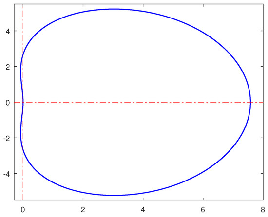
Figure 1. Region of absolute stability of the block hybrid method $y_{n+\frac{7}{4}}$.

Next, we describe how to plot the region of absolute stability of the second block hybrid method $y_{n+\frac{5}{2}}$. We begin by re-writting (20)–(23) in the following linear multi-step form:

$$\begin{array}{cc}\hfill \left[\begin{array}{cccc}1& 0& 0& 0\\ \\ 0& 1& 0& 0\\ \\ 0& 0& 1& 0\\ \\ 0& 0& 0& 1\end{array}\right]\left[\begin{array}{c}{y}_{n+1}\\ \\ y_{n+\frac{3}{2}}\\ \\ y_{n+2}\\ \\ y_{n+\frac{5}{2}}\end{array}\right]& =\left[\begin{array}{cccc}0& 0& 1& 0\\ \\ 0& 0& \frac{37}{496}& \frac{459}{496}\\ \\ 0& 0& -\frac{1}{31}& \frac{32}{31}\\ \\ 0& 0& \frac{621}{496}& -\frac{125}{496}\end{array}\right]\left[\begin{array}{c}{y}_{n-3}\\ \\ y_{n-2}\\ \\ y_n\\ \\ y_{n+1}\end{array}\right]+h\left[\begin{array}{cccc}0& 0& 0& \frac{269}{900}\\ \\ 0& 0& 0& \frac{39}{1984}\\ \\ 0& 0& 0& -\frac{1}{93}\\ \\ 0& 0& 0& \frac{735}{1984}\end{array}\right]\left[\begin{array}{c}{f}_{n-3}\\ \\ f_{n-2}\\ \\ f_{n-1}\\ \\ f_n\end{array}\right]\hfill \\ \hfill & +h\left[\begin{array}{cccc}\frac{68}{45}& -\frac{61}{45}& \frac{41}{60}& -\frac{31}{225}\\ \\ \frac{81}{248}& \frac{15}{62}& -\frac{27}{1984}& 0\\ \\ \frac{4}{31}& \frac{64}{93}& \frac{5}{31}& 0\\ \\ \frac{525}{248}& -\frac{75}{62}& \frac{2925}{1984}& 0\end{array}\right]\left[\begin{array}{c}{f}_{n+1}\\ \\ f_{n+\frac{3}{2}}\\ \\ f_{n+2}\\ \\ f_{n+\frac{5}{2}}\end{array}\right],\hfill \end{array}$$

where

$$P_1=\left[\begin{array}{cccc}1& 0& 0& 0\\ \\ 0& 1& 0& 0\\ \\ 0& 0& 1& 0\\ \\ 0& 0& 0& 1\end{array}\right],Q_1=\left[\begin{array}{cccc}0& 0& 1& 0\\ \\ 0& 0& \frac{37}{496}& \frac{459}{496}\\ \\ 0& 0& -\frac{1}{31}& \frac{32}{31}\\ \\ 0& 0& \frac{621}{496}& -\frac{125}{496}\end{array}\right],$$

$$R_1=\left[\begin{array}{cccc}0& 0& 0& \frac{269}{900}\\ \\ 0& 0& 0& \frac{39}{1984}\\ \\ 0& 0& 0& -\frac{1}{93}\\ \\ 0& 0& 0& \frac{735}{1984}\end{array}\right],\mathrm{and}{S}_1=\left[\begin{array}{cccc}\frac{68}{45}& -\frac{61}{45}& \frac{41}{60}& -\frac{31}{225}\\ \\ \frac{81}{248}& \frac{15}{62}& -\frac{27}{1984}& 0\\ \\ \frac{4}{31}& \frac{64}{93}& \frac{5}{31}& 0\\ \\ \frac{525}{248}& -\frac{75}{62}& \frac{2925}{1984}& 0\end{array}\right].$$

Using the above matrices, one obtains the stability polynomial $|P_{1}w-Q_1-R_{1}z-S_{1}zw|$. An application of Newton’s method in solving the corresponding stability polynomial equation and subsequent plot gives Figure 2, which is $A\left(\alpha \right)$-stable.

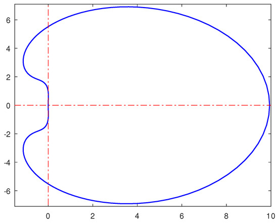
Figure 2. Region of absolute stability of the block hybrid method $y_{n+\frac{5}{2}}$.

Figure 1 and Figure 2 show the regions of absolute stability of the two hybrid methods and they are $A\left(\alpha \right)$-stable, albeit one has a larger region of absolute stability than the other. In both figures, the regions outside the contours represent the stable region while the region inside the contour correspond to the unstable region.

In the discussions underneath, we present Newton-based algorithms for the solution of systems of initial value problems since we have shown that the Jacobians are non-singular. We state clearly that both algorithms are self-starting and do not rely on predictors or correctors to start. The starting values are the initial values of the differential equations.

3.1. Algorithm for $y_{n+\frac{7}{4}}$

Input: h, tol, system of differential equations to be solved, their initial values and corresponding Jacobians.

For $k=1,2,3,\cdots ,$ until convergence

$$\mathrm{Form}{\mathbf{v}}^{\left(k\right)}=\left[\begin{array}{c}{y}_{n+1}^{\left(k\right)}\\ y_{n+\frac{3}{2}}^{\left(k\right)}\\ y_{n+2}^{\left(k\right)}\\ y_{n+\frac{5}{2}}^{\left(k\right)}\end{array}\right],$$

and

$$\mathbf{F}\left({\mathbf{v}}^{\left(k\right)}\right)=\left[\begin{array}{c}{y}_{n+1}-y_n-\frac{h}{630}\left[-179f_n-1169f_{n+1}+2156f_{n+\frac{3}{2}}-1984f_{n+\frac{7}{4}}+546f_{n+2}\right]\\ y_{n+\frac{3}{2}}-\frac{37}{496}{y}_n-\frac{459}{496}{y}_{n+1}-\frac{h}{1984}\left[39f_n+648f_{n+1}+480f_{n+\frac{3}{2}}-27f_{n+2}\right]\\ y_{n+\frac{7}{4}}-\frac{243}{7936}{y}_n-\frac{7693}{7936}{y}_{n+1}-\frac{h}{31744}\left[231f_n+7644f_{n+1}+16464f_{n+\frac{3}{2}}+441f_{n+2}\right]\\ y_{n+2}+\frac{1}{31}{y}_n-\frac{32}{31}{y}_{n+1}-\frac{h}{93}\left[-f_n+12f_{n+1}+64f_{n+\frac{3}{2}}+15f_{n+2}\right]\end{array}\right].$$

Compute $J_7\left({\mathbf{v}}^{\left(k\right)}\right)$.

Find the $PLU$ factorization of $J_7\left({\mathbf{v}}^{\left(k\right)}\right)$, i.e., $P{J}_7\left({\mathbf{v}}^{\left(k\right)}\right)=LU,$ P is a permutation matrix.

Solve $L{\mathbf{w}}^{\left(k\right)}=-P\mathbf{F}\left({\mathbf{v}}^{\left(k\right)}\right)$ for ${\mathbf{w}}^{\left(k\right)}$.

Solve for $\Delta {\mathbf{v}}^{\left(k\right)}$ in $U\Delta {\mathbf{v}}^{\left(k\right)}={\mathbf{w}}^{\left(k\right)}$.

Increment ${\mathbf{v}}^{(k+1)}={\mathbf{v}}^{\left(k\right)}+\Delta {\mathbf{v}}^{\left(k\right)}.$

Output: $y_{n+1}^{(k+1)}.$

We now present the second $y_{n+\frac{5}{2}}$ algorithm below.

3.2. Algorithm for $y_{n+\frac{5}{2}}$

Input: h, tol, system of differential equations to be solved, their initial values and corresponding Jacobians.

For $k=1,2,3,\cdots ,$ until convergence

$$\mathrm{Form}{\mathbf{v}}^{\left(k\right)}=\left[\begin{array}{c}{y}_{n+1}^{\left(k\right)}\\ y_{n+\frac{3}{2}}^{\left(k\right)}\\ y_{n+2}^{\left(k\right)}\\ y_{n+\frac{3}{2}}^{\left(k\right)}\end{array}\right],$$

and

$$\mathbf{F}\left({\mathbf{v}}^{\left(k\right)}\right)=\left[\begin{array}{c}{y}_{n+1}-y_n-\frac{h}{900}\left[269f_n+1360f_{n+1}-1220f_{n+\frac{3}{2}}-124f_{n+\frac{5}{2}}+615f_{n+2}\right]\\ y_{n+\frac{3}{2}}-\frac{37}{496}{y}_n-\frac{459}{496}{y}_{n+1}-\frac{h}{1984}\left[39f_n+648f_{n+1}+480f_{n+\frac{3}{2}}-27f_{n+2}\right]\\ y_{n+2}+\frac{1}{31}{y}_n-\frac{32}{31}{y}_{n+1}-\frac{h}{93}\left[-f_n+12f_{n+1}+64f_{n+\frac{3}{2}}+15f_{n+2}\right]\\ y_{n+\frac{5}{2}}-\frac{2484}{1984}{y}_n+\frac{500}{1984}{y}_{n+1}-\frac{h}{1984}\left[735f_n+4200f_{n+1}-2400f_{n+\frac{3}{2}}+2925f_{n+2}\right]\end{array}\right].$$

Compute $J_5\left({\mathbf{v}}^{\left(k\right)}\right)$.

Find the $PLU$ factorization of $J_5\left({\mathbf{v}}^{\left(k\right)}\right)$, i.e., $P{J}_5\left({\mathbf{v}}^{\left(k\right)}\right)=LU,$ P is a permutation matrix.

Solve $L{\mathbf{w}}^{\left(k\right)}=-P\mathbf{F}\left({\mathbf{v}}^{\left(k\right)}\right)$ for ${\mathbf{w}}^{\left(k\right)}$.

Solve $U\Delta {\mathbf{v}}^{\left(k\right)}={\mathbf{w}}^{\left(k\right)}$ for $\Delta {\mathbf{v}}^{\left(k\right)}$.

Increment ${\mathbf{v}}^{(k+1)}={\mathbf{v}}^{\left(k\right)}+\Delta {\mathbf{v}}^{\left(k\right)}.$

Output: $y_{n+1}^{(k+1)}.$

The stopping criterion for both algorithms is

$$\parallel \Delta {\mathbf{v}}^{\left(k\right)}\parallel \le \mathtt{tol}(1+\parallel {\mathbf{v}}^{\left(k\right)}\parallel ).$$

When the size of the matrix is rather large, the use of iterative solvers like GMRES is highly recommended. Next, we support our theoretical results with some numerical examples in the next section.

4. Numerical Experiments

In this section, we compare the performance of the two methods to see which is better. We compare the absolute errors of the exact solution with the numerical approximations as well as their respective cputimes. We used a 64-bit DELL Latitude laptop running on Intel(R) Core(TM) i5-5200U CPU @ 2.20GHz, manufactured in the USA, in all numerical computations. The first and last test problems were drawn from [35] with the sole aim of comparing the results of our method with theirs. The second test problem was from Chemistry. Throughout this section, we used a constant step size of $h=0.1$ on the same integration interval of $[0,50]$, as shown in Table 3, Table 4, Table 5, Table 6 and Table 7 and their respective figures. However, for the purpose of comparison with the work in [35], we extended the interval to $[0,500]$, as shown in Table 4 and Table 8.

Table 3. Absolute error of the block hybrid methods $y_{n+\frac{7}{4}}$ and $y_{n+\frac{5}{2}}$ on Example 1.

x	y	Absolute Error for ${\mathit{y}}_{\mathit{n}+\frac{7}{4}}$	Absolute Error for ${\mathit{y}}_{\mathit{n}+\frac{5}{2}}$
5	$y_1$	4.5935115213239299$\times {10}^{-07}$	4.4495405902951008$\times {10}^{-07}$
	$y_2$	4.8050326706232382$\times {10}^{-08}$	4.6460347875344754$\times {10}^{-08}$
10	$y_1$	2.0855112094424000$\times {10}^{-11}$	2.0201772875313122$\times {10}^{-11}$
	$y_2$	3.1704212170890252$\times {10}^{-10}$	3.0313075502139391$\times {10}^{-10}$
20	$y_1$	4.2987802361462157$\times {10}^{-20}$	4.1642371192651194$\times {10}^{-20}$
	$y_2$	1.3851474630459919$\times {10}^{-14}$	1.2925765285153073$\times {10}^{-14}$
30	$y_1$	8.8609023013571046$\times {10}^{-29}$	8.5838358912098099$\times {10}^{-29}$
	$y_2$	6.0424991742526876$\times {10}^{-19}$	5.4886853366277116$\times {10}^{-19}$
40	$y_1$	1.8264620443729859$\times {10}^{-37}$	1.7694054396306910$\times {10}^{-37}$
	$y_2$	2.6315790821435655$\times {10}^{-23}$	2.3195198529150539$\times {10}^{-23}$
50	$y_1$	3.7648125181410106$\times {10}^{-46}$	3.6473152891560397$\times {10}^{-46}$
	$y_2$	1.1440182168782429$\times {10}^{-27}$	9.7481843383636344$\times {10}^{-28}$

Table 4. Absolute error of the block hybrid methods, Yakubu et al. [35], $y_{n+\frac{7}{4}}$ and $y_{n+\frac{5}{2}}$ on Example 1.

x	y	Absolute Error in [35]	Absolute Error for ${\mathit{y}}_{\mathit{n}+\frac{7}{4}}$	Absolute Error for ${\mathit{y}}_{\mathit{n}+\frac{5}{2}}$
5	$y_1$	1.228938367083$\times {10}^{-03}$	4.5935115213239$\times {10}^{-07}$	4.4495405902951$\times {10}^{-07}$
	$y_2$	1.800318343625$\times {10}^{-06}$	4.8050326706232$\times {10}^{-08}$	4.6460347875344$\times {10}^{-08}$
50	$y_1$	3.325679258575$\times {10}^{-05}$	3.7648125181410$\times {10}^{-46}$	3.6473152891560$\times {10}^{-46}$
	$y_2$	5.804723043345$\times {10}^{-07}$	1.1440182168782$\times {10}^{-27}$	9.7481843383636$\times {10}^{-28}$
250	$y_1$	3.622719245691$\times {10}^{-12}$	0	0
	$y_2$	2.101212666995$\times {10}^{-10}$	0	0
500	$y_1$	7.173620185942$\times {10}^{-21}$	0	0
	$y_2$	9.350493168888$\times {10}^{-15}$	0	0

Table 5. Absolute error of the block hybrid methods $y_{n+\frac{7}{4}}$ and $y_{n+\frac{5}{2}}$ on Example 2.

x	y	Absolute Error for ${\mathit{y}}_{\mathit{n}+\frac{7}{4}}$	Absolute Error for ${\mathit{y}}_{\mathit{n}+\frac{5}{2}}$
5	$y_1$	1.8429201220637736$\times {10}^{-10}$	2.7234449417878892$\times {10}^{-10}$
	$y_2$	1.8429326120728007$\times {10}^{-10}$	2.7233922061942195$\times {10}^{-10}$
10	$y_1$	2.8917541972095506$\times {10}^{-11}$	4.4907285355610949$\times {10}^{-11}$
	$y_2$	2.8917645188142327$\times {10}^{-11}$	4.4906853409465430$\times {10}^{-11}$
20	$y_1$	3.8537197115081148$\times {10}^{-13}$	6.0765400957535354$\times {10}^{-13}$
	$y_2$	3.8537266910596002$\times {10}^{-13}$	6.0765109578201498$\times {10}^{-13}$
30	$y_1$	3.9031860015233805$\times {10}^{-15}$	6.1072016762397691$\times {10}^{-15}$
	$y_2$	3.9031907131441496$\times {10}^{-15}$	6.1071820886028638$\times {10}^{-15}$
40	$y_1$	3.5794145759740676$\times {10}^{-17}$	5.4886823015453322$\times {10}^{-17}$
	$y_2$	3.5794177192603953$\times {10}^{-17}$	5.4886691080145620$\times {10}^{-17}$
50	$y_1$	3.0204844833668178$\times {10}^{-19}$	4.6178900419926924$\times {10}^{-19}$
	$y_2$	3.0204866159418346$\times {10}^{-19}$	4.6178811401075847$\times {10}^{-19}$

Table 6. Absolute error of the block hybrid methods $y_{n+\frac{7}{4}}$ and $y_{n+\frac{5}{2}}$ on Example 3.

x	y	Absolute Error for ${\mathit{y}}_{\mathit{n}+\frac{7}{4}}$	Absolute Error for ${\mathit{y}}_{\mathit{n}+\frac{5}{2}}$
5	$y_1$	2.3285830553148310$\times {10}^{-22}$	2.2493291039341911$\times {10}^{-22}$
	$y_2$	1.3218783622033109$\times {10}^{-22}$	1.4477085626385313$\times {10}^{-22}$
	$y_3$	1.2354721309575536$\times {10}^{-23}$	1.7115476217234377$\times {10}^{-23}$
10	$y_1$	1.5438485820040401$\times {10}^{-44}$	1.5546760679948769$\times {10}^{-44}$
	$y_3$	5.0309547106817356$\times {10}^{-44}$	5.0285879396184281$\times {10}^{-44}$
	$y_2$	4.6131942308588293$\times {10}^{-45}$	6.3093549042213966$\times {10}^{-45}$
20	$y_1$	3.6580869562867370$\times {10}^{-88}$	3.6581192736544930$\times {10}^{-88}$
	$y_2$	1.9226360458970499$\times {10}^{-87}$	1.9226360578422238$\times {10}^{-87}$
	$y_3$	3.2194709960708681$\times {10}^{-88}$	4.2961763276024321$\times {10}^{-88}$
30	$y_1$	0	0
	$y_2$	0	0
	$y_3$	0	0
40	$y_1$	0	0
	$y_2$	0	0
	$y_3$	0	0
50	$y_1$	0	0
	$y_2$	0	0
	$y_3$	0	0

Table 7. Absolute error of the block hybrid methods $y_{n+\frac{7}{4}}$ and $y_{n+\frac{5}{2}}$ on Example 4.

x	y	Absolute Error for ${\mathit{y}}_{\mathit{n}+\frac{7}{4}}$	Absolute Error for ${\mathit{y}}_{\mathit{n}+\frac{5}{2}}$
5	$y_1$	2.6069389501515157$\times {10}^{-22}$	2.6069389501515157$\times {10}^{-22}$
	$y_2$	8.0250935335644924$\times {10}^{-23}$	8.0250935335644924$\times {10}^{-23}$
	$y_3$	8.6744998698744801$\times {10}^{-13}$	1.2898041482202381$\times {10}^{-12}$
	$y_4$	8.8587245265087100$\times {10}^{-10}$	1.3666554329189173$\times {10}^{-09}$
	$y_5$	1.7596617218895716$\times {10}^{-10}$	2.7328000973270150$\times {10}^{-10}$
	$y_6$	8.6153306710912148$\times {10}^{-14}$	1.3411494137471891$\times {10}^{-13}$
10	$y_1$	5.1681476049220830$\times {10}^{-44}$	5.1681476049220830$\times {10}^{-44}$
	$y_2$	9.8396182267041682$\times {10}^{-45}$	9.8396182267041682$\times {10}^{-45}$
	$y_3$	3.5751428964356635$\times {10}^{-21}$	5.3153053899417913$\times {10}^{-21}$
	$y_4$	1.1937922479439249$\times {10}^{-11}$	1.8416901846878692$\times {10}^{-11}$
	$y_5$	2.8888368260038266$\times {10}^{-11}$	4.4864376970432662$\times {10}^{-11}$
	$y_6$	1.0447198661722723$\times {10}^{-13}$	1.6314727346866675$\times {10}^{-13}$
20	$y_1$	7.7855244617256059$\times {10}^{-88}$	7.7855244617256059$\times {10}^{-88}$
	$y_2$	1.7956044336063368$\times {10}^{-87}$	1.7956044336063368$\times {10}^{-87}$
	$y_3$	3.0364165427948283$\times {10}^{-38}$	4.5134348071673213$\times {10}^{-38}$
	$y_4$	1.0839615410958194$\times {10}^{-15}$	1.6722517595367738$\times {10}^{-15}$
	$y_5$	3.8929657295103809$\times {10}^{-13}$	6.0458761478102141$\times {10}^{-13}$
	$y_6$	7.6882944455292090$\times {10}^{-14}$	1.2007062011321068$\times {10}^{-13}$
30	$y_1$	0	0
	$y_2$	0	0
	$y_3$	1.9341519135769713$\times {10}^{-55}$	2.8744015994507605$\times {10}^{-55}$
	$y_4$	7.3817656946758547$\times {10}^{-20}$	1.1388014559059823$\times {10}^{-19}$
	$y_5$	3.9345892715868008$\times {10}^{-15}$	6.1105188160798945$\times {10}^{-15}$
	$y_6$	4.2445214010200516$\times {10}^{-14}$	6.6252558994506217$\times {10}^{-14}$
40	$y_1$	0	0
	$y_2$	0	0
	$y_3$	1.0951341397262779$\times {10}^{-72}$	1.6271787057567443$\times {10}^{-72}$
	$y_4$	4.4684213318548600$\times {10}^{-24}$	6.8935327550012643$\times {10}^{-24}$
	$y_5$	3.5348071243628592$\times {10}^{-17}$	5.4896470009347222$\times {10}^{-17}$
	$y_6$	2.0799334476961917$\times {10}^{-14}$	3.2505248492853411$\times {10}^{-14}$
50	$y_1$	0	0
	$y_2$	0	0
	$y_3$	5.8132012201935056$\times {10}^{-90}$	8.6356372622664460$\times {10}^{-90}$
	$y_4$	2.5358248498385642$\times {10}^{-28}$	3.9120729933952014$\times {10}^{-28}$
	$y_5$	2.9771677973414147$\times {10}^{-19}$	4.6236187847225050$\times {10}^{-19}$
	$y_6$	9.5591937143701955$\times {10}^{-15}$	1.4946377469016170$\times {10}^{-14}$

Table 8. Absolute error of the block hybrid methods, Yakubu et al. [35], $y_{n+\frac{7}{4}}$ and $y_{n+\frac{5}{2}}$ on Example 4.

x	y	Absolute Error in [35]	Absolute Error for ${\mathit{y}}_{\mathit{n}+\frac{7}{4}}$	Absolute Error for ${\mathit{y}}_{\mathit{n}+\frac{5}{2}}$
5	$y_1$	2.220446049250$\times {10}^{-16}$	2.6069389501515$\times {10}^{-22}$	2.6069389501515$\times {10}^{-22}$
	$y_2$	1.318389841742$\times {10}^{-16}$	8.0250935335644$\times {10}^{-23}$	8.0250935335644$\times {10}^{-23}$
	$y_3$	0	8.6744998698744$\times {10}^{-13}$	1.2898041482202$\times {10}^{-12}$
	$y_4$	0	8.8587245265087$\times {10}^{-10}$	1.3666554329189$\times {10}^{-09}$
50	$y_1$	3.330669073875$\times {10}^{-16}$	0	0
	$y_2$	7.771561172376$\times {10}^{-16}$	0	0
	$y_3$	4.440892098500$\times {10}^{-16}$	5.8132012201935$\times {10}^{-90}$	8.6356372622664$\times {10}^{-90}$
	$y_4$	1.110223024625$\times {10}^{-16}$	2.5358248498385$\times {10}^{-28}$	3.9120729933952$\times {10}^{-28}$
250	$y_1$	6.591949208711$\times {10}^{-17}$	0	0
	$y_2$	1.734723475976$\times {10}^{-18}$	0	0
	$y_3$	8.326672684688$\times {10}^{-17}$	0	0
	$y_4$	6.661338147750$\times {10}^{-16}$	0	0
500	$y_1$	6.810144895924$\times {10}^{-19}$	0	0
	$y_2$	2.710505431213$\times {10}^{-20}$	0	0
	$y_3$	4.857225732735$\times {10}^{-17}$	0	0
	$y_4$	3.330669073875$\times {10}^{-16}$	0	0

Example 1. 

The non-linear stiff Kaps problem [36]

$$\left[\begin{array}{c}{y}_1^{\prime }\left(x\right)\\ \\ y_2^{\prime }\left(x\right)\end{array}\right]=\left[\begin{array}{c}-1002y_1\left(x\right)-1000y_2^2\left(x\right)\\ \\ y_1\left(x\right)-y_2\left(x\right)-y_2^2\left(x\right)\end{array}\right]\mathit{such}\mathit{that}{y}_1\left(0\right)=1,y_2\left(0\right)=1.$$

The analytic solution is $y_1\left(x\right)=exp(-2x)$ and $y_2\left(x\right)=exp(-x)$.

The results of the numerical experiments for this example are presented in Table 3 and Table 4 and Figure 3. Table 3 showed that the block hybrid method $y_{n+\frac{5}{2}}$ performed better than $y_{n+\frac{7}{4}}$ using the same initial conditions, especially for $x=50$. Nevertheless, both methods, though of order five, outperformed Yakubu et al.’s [35] fourteenth-order method, as summarized in Table 4. Figure 3, which is a log–log plot of the errors and step sizes, showed that, while both methods performed at par for $y_1\left(x\right)$, the same was not the case for $y_2\left(x\right)$ because $y_{n+\frac{7}{4}}$ performed better than $y_{n+\frac{5}{2}}$.

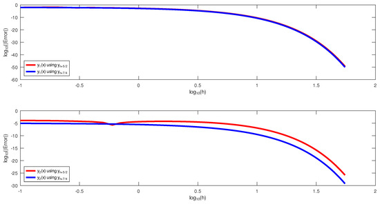
Figure 3. The log–log plots of the errors and the step size on Example 1.

Example 2. 

The Wu problem [37] arises from Chemistry

$$\left[\begin{array}{c}{y}_1^{\prime }\left(x\right)\\ \\ y_2^{\prime }\left(x\right)\end{array}\right]=\left[\begin{array}{c}-500000y_1\left(x\right)+499999.5y_2\left(x\right)\\ \\ 499999.5y_1\left(x\right)-500000y_2\left(x\right)\end{array}\right]\mathit{with}\mathit{initial}\mathit{conditions}{y}_1\left(0\right)=0,y_2\left(0\right)=2.$$

The analytic solution is $y_1\left(x\right)=exp(-\frac{x}{2})-exp(-999999.5x)$ and $y_2\left(x\right)=exp(-\frac{x}{2})+exp(-999999.5x)$.

The results of the numerical experiments for this example are presented in Table 5 and Figure 4. Table 5 showed that the block hybrid method $y_{n+\frac{5}{2}}$ performed at par with $y_{n+\frac{7}{4}}$ using the same initial conditions. However, a plot of the log–log of the error and step size showed that $y_{n+\frac{5}{2}}$ outperformed $y_{n+\frac{7}{4}}$.

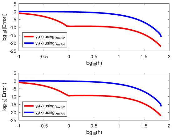
Figure 4. The log−log plots of the errors and the step size on Example 2.

Example 3. 

We consider the following three-dimensional linear problem:

$$\left[\begin{array}{c}{y}_1^{\prime }\left(x\right)\\ \\ y_2^{\prime }\left(x\right)\\ \\ y_3^{\prime }\left(x\right)\end{array}\right]=\left[\begin{array}{ccc}-10& 21& 0\\ \\ -21& -10& 0\\ \\ 0& 0& -10\end{array}\right]\left[\begin{array}{c}{y}_1\left(x\right)\\ \\ y_2\left(x\right)\\ \\ y_3\left(x\right)\end{array}\right],$$

with initial condition $[y_1\left(0\right),y_2\left(0\right),y_3\left(0\right)]=[1,1,1]$. The analytic solution is

$$\left[\begin{array}{c}{y}_1\left(x\right)\\ y_2\left(x\right)\\ y_3\left(x\right)\end{array}\right]=\left[\begin{array}{c}exp(-10x)\left(cos\left(21x\right)+sin\left(21x\right)\right)\\ exp(-10x)\left(cos\left(21x\right)-sin\left(21x\right)\right)\\ exp(-10x)\end{array}\right].$$

The results of the numerical experiments for this example are presented in Table 6 and Figure 5. Table 6 showed that the block hybrid method $y_{n+\frac{7}{4}}$ performed at par with $y_{n+\frac{5}{2}}$ using the same initial values. In addition, this is confirmed by the log–log plots of the error and step size in Figure 5.

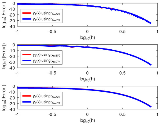
Figure 5. The log–log plots of the errors and the step size on Example 3.

Example 4. 

The linear stiff IVPs considered by Fatunla [38].

$$\left[\begin{array}{c}{y}_1^{\prime }\left(x\right)\\ \\ y_2^{\prime }\left(x\right)\\ \\ y_3^{\prime }\left(x\right)\\ \\ y_4^{\prime }\left(x\right)\\ \\ y_5^{\prime }\left(x\right)\\ \\ y_6^{\prime }\left(x\right)\end{array}\right]=\left[\begin{array}{ccccc}-10& 100& 0& 0& 0\\ \\ -100& -10& 0& 0& 0& 0\\ \\ 0& 0& -4& 0& 0& 0\\ \\ 0& 0& 0& -1& 0& 0\\ \\ 0& 0& 0& 0& -0.5& 0\\ \\ 0& 0& 0& 0& 0& -0.1\end{array}\right]\left[\begin{array}{c}{y}_1\left(x\right)\\ \\ y_2\left(x\right)\\ \\ y_3\left(x\right)\\ \\ y_4\left(x\right)\\ \\ y_5\left(x\right)\\ \\ y_6\left(x\right)\end{array}\right],\left[\begin{array}{c}{y}_1\left(0\right)\\ \\ y_2\left(0\right)\\ \\ y_3\left(0\right)\\ \\ y_4\left(0\right)\\ \\ y_5\left(0\right)\\ \\ y_6\left(0\right)\end{array}\right]=\left[\begin{array}{c}1\\ \\ 1\\ \\ 1\\ \\ 1\\ \\ 1\\ \\ 1\end{array}\right].$$

The results of the numerical experiments for this example are presented in Table 7 and Figure 6. Table 7 and Figure 6 showed that the block hybrid method $y_{n+\frac{5}{2}}$ performed at par with those of $y_{n+\frac{7}{4}}$ using the same initial conditions. Nevertheless, both methods, though of order five, outperformed Yakubu et al.’s [35] fourteenth-order method, as shown in Table 8.

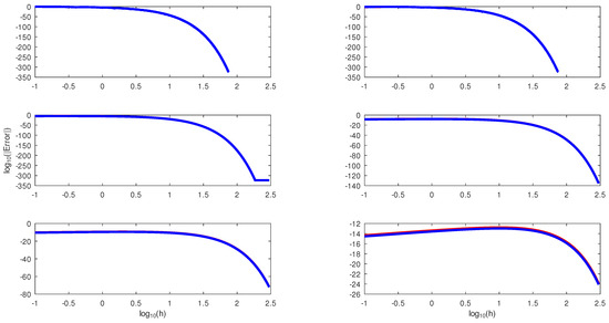
Figure 6. The log–log plots of the errors and the step size on Example 4. The red and blue lines represents $y_{n+\frac{5}{2}}$ and $y_{n+\frac{7}{4}}$, respectively.

From Table 9, we observed that the Wu problem of Example 2 was ill-conditioned at 1,072,275.37 for $y_{n+\frac{7}{4}}$ versus 652,920 for $y_{n+\frac{5}{2}}$. Upon inspection, it was discovered that the increase in the condition number of the system was due to the ill-conditioning of the Jacobian matrix of the problem under consideration with a condition number of $2\times {10}^6$. The same table shows that, in Examples 1–3, the condition numbers for $y_{n+\frac{7}{4}}$ are, respectively, 1.72, 3 and 2 times that for $y_{n+\frac{5}{2}}$.

Table 9. Comparing the condition number and cputime for both block hybrid methods under discussion. Here, $\kappa \left(J_7\right)$ and $\kappa \left(J_5\right)$ are the condition numbers of the Jacobians $J_7$ and $J_5$ at the root, respectively.

Example	Size of System	$\mathit{\kappa }\left({\mathit{J}}_7\right)$	$\mathit{\kappa }\left({\mathit{J}}_5\right)$	cputime$\left({\mathit{y}}_{\mathit{n}+\frac{7}{4}}\right)$	cputime$\left({\mathit{y}}_{\mathit{n}+\frac{5}{2}}\right)$
Example 1	8$\times 8$	1091.10	633.14	3.6000$\times {10}^{-5}$	3.6000$\times {10}^{-5}$
Example 2	8$\times 8$	1,072,275.37	652,920.00	3.6000$\times {10}^{-5}$	3.6666$\times {10}^{-5}$
Example 3	12$\times 12$	67.65	22.11	5.7000$\times {10}^{-5}$	5.8000$\times {10}^{-5}$
Example 4	24$\times 24$	137.34	68.07	3.9333$\times {10}^{-5}$	3.9333$\times {10}^{-5}$

We remark that, in order to reduce the condition number and accuracy, we also tried at the off-grid point $\frac{5}{4}$ to derive a new block hybrid method. However, this resulted in a higher condition number than both $y_{n+\frac{7}{4}}$ and $y_{n+\frac{5}{2}}$. On a final note, the results of both methods presented in this study outperform the second-order and fourteenth-order second derivative method of [35] with less function evaluations and computational time.

5. Conclusions

As shown in the numerical examples in this study, we have confirmed that, for higher-dimensional systems of initial value, the problems $y_{n+\frac{5}{2}}$ still have a lower condition number in agreement with one-dimensional initial value problems. It was also observed that, for higher-dimensional systems, the result of numerical experiments showed that $y_{n+\frac{5}{2}}$ performed favorably well in comparison to the exact solution $y_{n+\frac{7}{4}}$. Therefore, we recommend the block hybrid method $y_{n+\frac{5}{2}}$ for the numerical integration of systems of linear, nonlinear, stiff and non-stiff differential equations due to its better conditioning and accuracy.

References

- Shampine, L.F. Ill-conditioned matrices and the integration of stiff ODEs. J. Comput. Appl. Math. 1993, 48, 279–292. [Google Scholar] [CrossRef]
- Trefethen, L.N.; Bau, D., III. Numerical Linear Algebra; SIAM: Philadelphia, PA, USA, 1997. [Google Scholar]
- Butcher, J.C. A multistep generalization of Runge-Kutta method with four or five stages. J. Ass. Comput. Mach. 1967, 14, 84–99. [Google Scholar] [CrossRef]
- Butcher, J.C. Numerical methods for ordinary differential equations in the 20th century. J. Comput. Appl. Math. 2000, 125, 1–29. [Google Scholar] [CrossRef]
- Butcher, J.C. Numerical Methods for Ordinary Differential Equations; John Wiley and Sons Ltd.: Oxford, UK, 2016. [Google Scholar]
- Akinola, R.O.; Ajibade, K.J. A proof of the non singularity of the D matrix used in deriving the two-step Butcher’s hybrid scheme for the solution of initial value problems. J. Appl. Math. Phys. 2021, 9, 3177–3201. [Google Scholar] [CrossRef]
- Akinola, R.O.; Shokri, A.; Yao, S.-W.; Kutchin, S.Y. Circumventing ill-conditioning arising from using linear multistep methods in approximating the solution of initial value problems. Mathematics 2022, 10, 2910. [Google Scholar] [CrossRef]
- Sirisena, U.W.; Kumleng, G.M.; Yahaya, Y.A. A new Butcher type two-step block hybrid multistep method for accurate and efficient parallel solution of ordinary differential equations. Abacus Math. Ser. 2004, 31, 1–7. [Google Scholar]
- Golub, G.H.; Wilkinson, J.H. Ill-conditioned eigensystems and the computation of the Jordan canonical form. SIAM Rev. 1976, 18, 578–619. [Google Scholar] [CrossRef]
- Peters, G.; Wilkinson, J.H. Inverse iteration, ill conditioned equations and Newton’s method. J. SIAM Rev. 1979, 21, 339–360. [Google Scholar] [CrossRef]
- Farooq, M.; Salhi, A. Improving the solvability of Ill-conditioned systems of linear equations by reducing the condition number of their matrices. J. Korean Math. Soc. 2011, 48, 939–952. [Google Scholar] [CrossRef]
- Douglas, C.C.; Lee, L.; Yeung, M. On solving ill conditioned linear systems. Procedia Comput. Sci. 2016, 80, 941–950. [Google Scholar] [CrossRef]
- Demmel, J.W. Applied Numerical Linear Algebra; Society for Industrial and Applied Mathematics: Philadelphia, PA, USA, 1997. [Google Scholar]
- Akram, G.; Elahi, Z.; Siddiqi, S.S. Use of Laguerre Polynomials for Solving System of Linear Differential Equations. Appl. Comput. Math. 2022, 21, 137–146. [Google Scholar]
- Khankishiyev, Z.F. Solution of one problem for a loaded differential equation by the method of finite differences. Appl. Comput. Math. 2022, 21, 147–157. [Google Scholar]
- Juraev, D.A.; Shokri, A.; Marian, D. Solution of the ill-posed Cauchy problem for systems of elliptic type of the first order. Fractal Fract. 2022, 6, 358. [Google Scholar] [CrossRef]
- Adee, S.O.; Atabo, V.O. Improved two-point block backward differentiation formulae for solving first order stiff initial value problems of ordinary differential equations. Niger. Ann. Pure Appl. Sci. 2020, 3, 200–209. [Google Scholar] [CrossRef]
- Antczak, T.; Arana-Jimenez, M. Optimality and duality results for new classes of nonconvex quasidifferentiable vector optimization problems. Appl. Comput. Math. 2022, 21, 21–34. [Google Scholar]
- Qi, F. Necessary and sufficient conditions for a difference defined by four derivatives of a function containing trigamma function to be completely monotonic. Appl. Comput. Math. 2022, 21, 61–70. [Google Scholar]
- Iskandarov, S.; Komartsova, E. On the influence of integral perturbations on the boundedness of solutions of a fourth-order linear differential equation. TWMS J. Pure Appl. Math. 2022, 13, 3–9. [Google Scholar]
- Mansour, M.A.; Lahrache, J.; El Ayoubi, A.; El Bekkali, A. The stability of parametric Cauchy problem of initial-value ordinary differential equation revisited. J. Appl. Numer. Optim. 2023, 5, 111–124. [Google Scholar]
- Ren, J.; Bai, L.; Zhai, C. A decreasing operator method for a fractional initial value problem on finite interval. J. Nonlinear Funct. Anal. 2023, 2023, 35. [Google Scholar]
- Hamidov, S.I. Optimal trajectories in reproduction models of economic dynamics. TWMS J. Pure Appl. Math. 2022, 13, 16–24. [Google Scholar]
- Akbay, A.; Turgay, N.; Ergüt, M. On Space-like Generalized Constant Ratio Hypersufaces in Minkowski Spaces. TWMS J. Pure Appl. Math. 2022, 13, 25–37. [Google Scholar]
- Juraev, D.A.; Shokri, A.; Marian, D. Regularized solution of the Cauchy problem in an unbounded domain. Symmetry 2022, 14, 1682. [Google Scholar] [CrossRef]
- Onumanyi, P.; Awoyemi, D.O.; Jator, S.N.; Sirisena, U.W. New Linear Multistep Methods with Continuous Coefficients for First Order Initial Value Problems. J. Niger. Math. Soc. 1994, 13, 37–51. [Google Scholar]
- Keller, H.B. Numerical Solution of Bifurcation and Nonlinear Eigenvalue Problems. In Applications of Bifurcation Theory; Rabinowitz, P., Ed.; Academic Press: New York, NY, USA, 1997; pp. 359–384. [Google Scholar]
- Spence, A.; Poulton, C. Photonic band structure calculations using nonlinear eigenvalue techniques. J. Comput. Phys. 2005, 204, 65–81. [Google Scholar] [CrossRef][Green Version]
- Akinola, R.O.; Freitag, M.A.; Spence, A. A method for the computation of Jordan blocks in parameter-dependent matrices. IMA J. Numer. Anal. 2014, 34, 955–976. [Google Scholar] [CrossRef][Green Version]
- Freitag, M.A.; Spence, A. A Newton-based method for the calculation of the distance to instability. Linear Algebra Appl. 2011, 435, 3189–3205. [Google Scholar] [CrossRef]
- Akinola, R.O.; Spence, A. A comparison of the Implicit Determinant Method and Inverse Iteration. J. Niger. Math. Soc. 2014, 33, 205–230. [Google Scholar]
- Lambert, J.D. Computational Methods in Ordinary Differential Equations; John Wiley: New York, NY, USA, 1973. [Google Scholar]
- Demmel, J.W. Discrete Variable Methods in Ordinary Differential Equations; John Wiley: New York, NY, USA, 1962. [Google Scholar]
- Widlund, O.B. A note on unconditionally stable linear multistep methods. BIT Numer. Math. 1967, 7, 65–70. [Google Scholar] [CrossRef]
- Yakubu, D.G.; Shokri, A.; Kumleng, G.M.; Marian, D. Second derivative block hybrid methods for the the numerical integration of differential systems. Fractal Fract. 2022, 6, 386. [Google Scholar] [CrossRef]
- Kaps, P.; Poon, S.W.H.; Bui, T.D. Rosenbrock methods for Stiff ODEs: A comparison of Richardson extrapolation and embedding technique. Pac. J. Sci. Technol. 1985, 34, 17–40. [Google Scholar] [CrossRef]
- Wu, X.Y.; Xiu, J.L. Two low accuracy methods for Stiff systems. Appl. Math. Comput. 2001, 123, 141–153. [Google Scholar] [CrossRef]
- Fatunla, S.O. Numerical integrators for stiff and highly oscillatory differential equations. J. Math. Comput. 1980, 34, 373–390. [Google Scholar] [CrossRef]
Disclaimer/Publisher’s Note: The statements, opinions and data contained in all publications are solely those of the individual author(s) and contributor(s) and not of MDPI and/or the editor(s). MDPI and/or the editor(s) disclaim responsibility for any injury to people or property resulting from any ideas, methods, instructions or products referred to in the content. |
© 2024 by the authors. Licensee MDPI, Basel, Switzerland. This article is an open access article distributed under the terms and conditions of the Creative Commons Attribution (CC BY) license (https://creativecommons.org/licenses/by/4.0/).