Abstract
In this paper, we examine the interplay between the structural and spectral properties of the unit graph for , where are distinct primes and are positive integers such that at least one of the must be greater than 1. We first analyze the structure of the unit graph of , treating it as what we will define as a ‘generalized join graph’ under these conditions. We then determine the Laplacian spectrum of and deduce that it is integral for all n. Consequently, we obtain the Laplacian spectral radius and algebraic connectivity of . We also prove that the vertex connectivity of is , where . We deduce the vertex connectivity of when , where are primes and are positive integers. Finally, we present conjectures regarding the vertex connectivity of when and , where are distinct primes, are positive integers, and .
Keywords:
unit graph; G-generalized join graph; Laplacian spectral radius; algebraic connectivity; ring of integers modulo n MSC:
05C25; 05C50; 05C75
1. Introduction
For any positive integer n, represents the ring of integers modulo n. The elements of this ring are denoted as . A nonzero element is considered a unit if x is coprime with n, meaning . In 1990, Grimaldi [1] introduced the concept of the unit graph for the ring . The unit graph is constructed by taking all elements of as vertices, with two distinct vertices x and y being adjacent if and only if is a unit in . Grimaldi analyzed the fundamental properties of , including the vertex degrees, covering numbers, independence numbers, Hamiltonian cycles, and chromatic polynomials. Additional studies on can be found in [2,3,4]. Ashrafi et al. subsequently extended the notion of unit graphs from to , where R is an arbitrary ring [5]. Their work examined features such as the diameter, planarity, chromatic index, and girth of . Other research contributions related to unit graphs over rings are documented in [6,7,8,9].
In recent years, the Laplacian spectrum and vertex connectivity of graphs related to algebraic structures have garnered significant attention from researchers. In 2020, Chattopadhyay et al. [10] investigated the Laplacian spectrum and vertex connectivity of the zero divisor graph associated with the ring . Further studies on the Laplacian spectrum and vertex connectivity of graphs connected to can be found in [11,12]. Shen et al. [3] examined the Laplacian spectrum of unit graphs when , where q is an odd prime and is a positive integer. They demonstrated that the vertex connectivity and algebraic connectivity of coincide if and only if . Moreover, they explored properties such as the Laplacian spectral radius and Laplacian integrality of .
In this paper, we explore the structure of and use it as a foundation to analyze the Laplacian spectrum and vertex connectivity of for various values of n. This paper is arranged as follows: In Section 2, we provide the preliminary concepts and results that are used throughout this paper. In Section 3, we examine the structure of for , where are distinct primes and are positive integers such that at least one of the must be greater than 1. We prove that is a generalized join graph. In Section 4, we investigate the Laplacian spectrum of , establishing that it is the Laplacian integral. Additionally, we derive the algebraic connectivity and the Laplacian spectral radius of . In Section 5, we investigate the vertex connectivity of and , where are primes and r and s are positive integers, based on their structure and Menger’s theorem. Lastly, we conjecture formulas for the vertex connectivity of for odd n.
2. Preliminaries
In this section, we present fundamental definitions and results that are necessary for the following sections. Consider a graph G with a vertex set and an edge set . For , two vertices and in G are said to be adjacent (or neighbors) if they are connected by an edge e in G. This adjacency is denoted by . For , let represent the set of all vertices in G that are adjacent to v. The degree of a vertex v, denoted as , is defined as the number of edges incident to v. A path in a graph is a sequence of distinct vertices where each vertex in the sequence is connected to the subsequent vertex by an edge. A graph G is considered connected if there exists a path between any two vertices in G. A complete graph is a graph where every pair of distinct vertices is connected by an edge. The complete graph containing n vertices is denoted by . A null graph is a graph consisting of n vertices and no edges. An isomorphism between two graphs, and , denoted by , is defined as a bijective mapping from to , such that in if and only if in . For two graphs, and , with disjoint vertex sets, the join is constructed by combining and and adding edges connecting every vertex in to each vertex in .
Let R be a ring with unity, and let denote the set of all units in R. The unit graph of a ring R is defined as the graph where the vertices correspond to all elements of R. Two distinct vertices, x and y, are adjacent if and only if their sum, , is a unit in R. Let R be a commutative ring with unity. An element is called nilpotent if there exists an integer such that . The nilradical of R, denoted as , is defined as the set of all nilpotent elements in R. Alternatively, it can also be characterized as the intersection of all prime ideals in R. A maximal ideal of R is an ideal such that no proper ideal I in R exists with . The Jacobson radical of a ring R is the set obtained by taking the intersection of all maximal ideals contained within R. Every maximal ideal in R is also a prime ideal. So, . Recall that, the sum of a nilpotent element and a unit is always a unit.
For a finite, simple, undirected graph G, the adjacency matrix is an matrix where the -th entry is 1 if , and 0 otherwise. The Laplacian matrix of a graph G is defined as , where is a diagonal matrix , with representing the degrees of the vertices in G. The second smallest eigenvalue of is called the algebraic connectivity, represented by . The value is greater than zero if and only if the graph G is connected. The largest eigenvalue of is referred to as the Laplacian spectral radius, denoted by . A graph G is said to be the Laplacian integral if all the eigenvalues of its Laplacian matrix are integers. Additional information on the Laplacian matrix of graphs is available in [13,14].
The spectrum of an matrix C, denoted as , represents the multiset of all its eigenvalues. If the distinct eigenvalues of C are with respective multiplicities , the spectrum of C is expressed as follows:
For a graph G, the Laplacian spectrum refers to the spectrum of its Laplacian matrix , commonly denoted as . For example:
Consider a graph G with k vertices, , and let be k pairwise disjoint graphs. The G-generalized join graph, denoted as , is constructed by replacing each vertex of G with the graph , and then adding edges between every vertex in and every vertex of whenever in G [15]. This result is instrumental for subsequent analysis.
Theorem 1
([16]). Consider a graph G with k vertices, , and let be k pairwise disjoint graphs containing vertices, respectively. Then we have the following:
where
and
In (2), indicates the multiset with a single occurrence of the eigenvalue 0 removed. Additionally, denotes the operation of adding to each element in
In this paper, are used to denote distinct prime numbers, while represent positive integers. Let n be a positive integer. Euler’s totient function, , calculates the number of integers from 1 to n that are coprime to n. Recall that and . Fakieh et al. examined the Laplacian spectrum of unit graphs corresponding to the ring [4]. This result is the main tool to prove Theorem 4.
Theorem 2
([4]). Let be distinct primes and k be a positive integer, .
- 1.
- If , then we have the following:
- 2.
- If , then we have the following:
The vertex connectivity of a graph G is defined as the minimum number of vertices that need to be removed from G to produce either a disconnected graph or a trivial graph. Fiedler presented a famous result that establishes a relation between vertex connectivity and algebraic connectivity as in [17]. A set of two or more paths in G is considered internally disjoint if no vertex in G serves as an internal vertex for more than one path in the set. Menger’s theorem provides a fundamental result related to vertex connectivity . It states that the minimum number of vertices that must be deleted to eliminate all -paths in G is equal to the maximum number of internally disjoint -paths, where x and y are nonadjacent vertices [18]. In other words, we have the following:
This paper uses Menger’s theorem to examine the vertex connectivity of .
3. as a Generalized Join Graph
Any integer can be written in the following form: . In this section and the next, we assume that at least one of the . In this case, note that is nontrivial. We prove that is a generalized join graph. To this end, we first study the structure of . Denote the maximal ideal of by , where is the ideal generated by the prime divisor of n, that is, . So, . Put , then we have the following:
Let S be the set of distinct representatives of . For , we denote the following:
The cosets of form a partition of the vertex set of . Thus, we have the following:
Let . Then, for , we have the following:
The next result describes the adjacency criterion for vertices in , where is described in Equation (3).
Lemma 1.
For , every vertex of is adjacent to every vertex of in if and only if .
Proof.
Clear.
Suppose that . Let and , which can be written as and , where . Now, . Here, is a unit by assumption, and is nilpotent. So, is a unit and, hence, every vertex of is adjacent to every vertex of in . □
By using parts (b) and (c) of Lemma 2.7 in [5] and Lemma 1, the following is evident:
Corollary 1.
The following statements hold:
- 1.
- For , the induced subgraph of is either or . Indeed, is if and only if .
- 2.
- For with , each vertex in is either adjacent to all vertices in or to none of them in .
The above result implies that the partition of of forms an equitable partition. This means that every vertex in has the same number of neighbors in for all .
We define by the simple graph whose vertices are the distinct representatives of , that is, the set of vertices is S, and in which two distinct vertices i and j are adjacent if and only if . The graph serves a pivotal role throughout the remainder of this paper.
Lemma 2.
.
Proof.
We define a map such that . Clearly, is well-defined and bijection. From Lemma 1, the adjacency relationships are preserved by . As a result, the conclusion is validated. □
The following lemma states that can be expressed as a generalized join graph.
Lemma 3.
Let be the induced subgraph of for . Then, we have the following:
Proof.
Replace each vertex i of with for . Consequently, the result is derived from Lemma 1 and Corollary 1. □
Example 1.
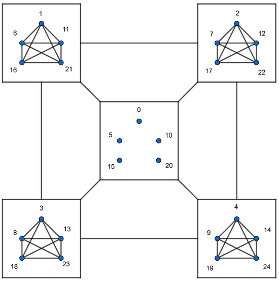
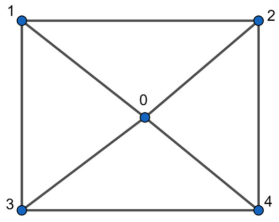
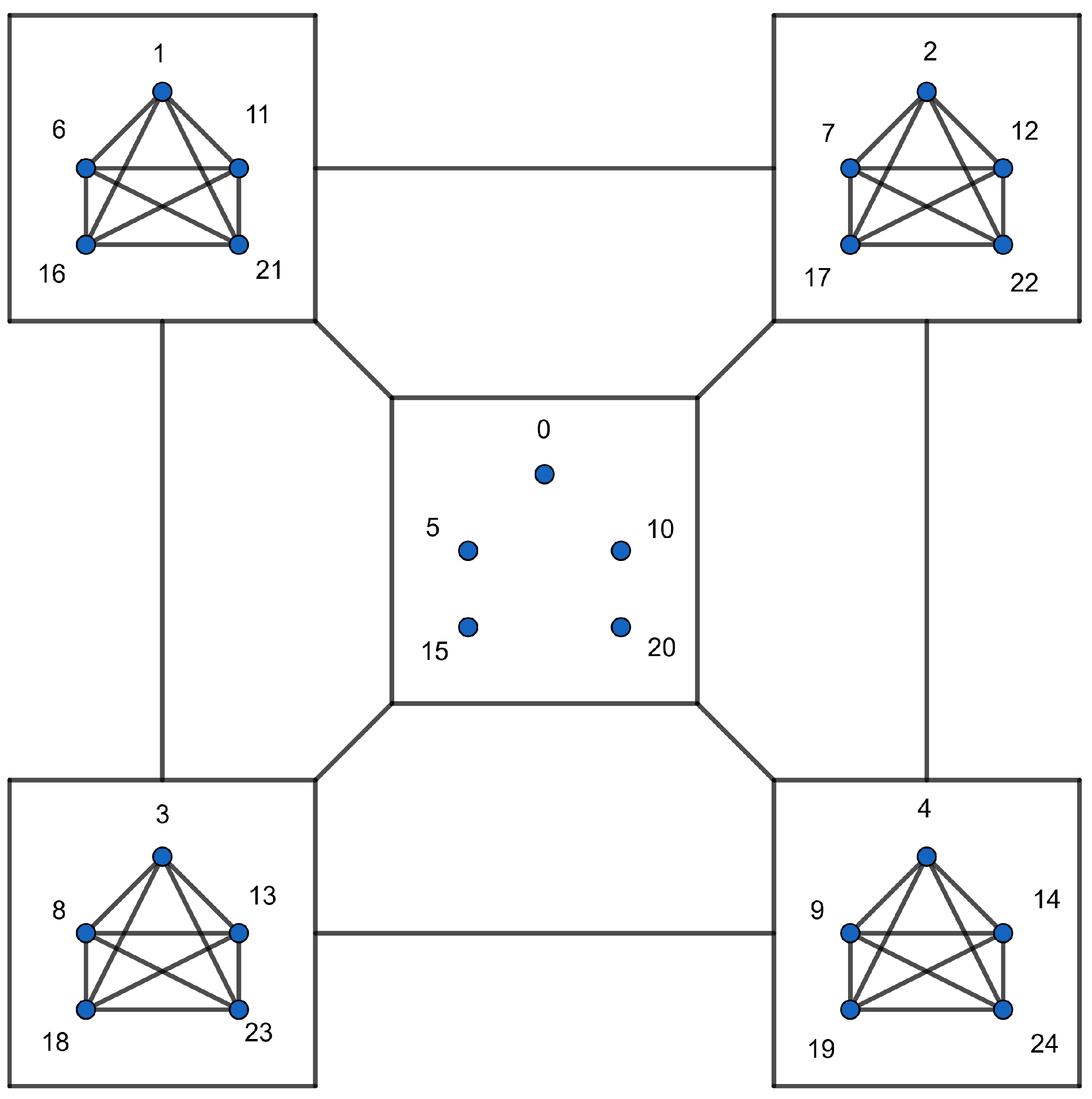
The unit graph , as illustrated in Figure 1, can be expressed using Lemma 3 as follows:
where is depicted in Figure 2, , and for . In Figure 1, the lines connecting two squares indicate that every vertex in one square is adjacent to all vertices in the other square.
Figure 1.
The graph .
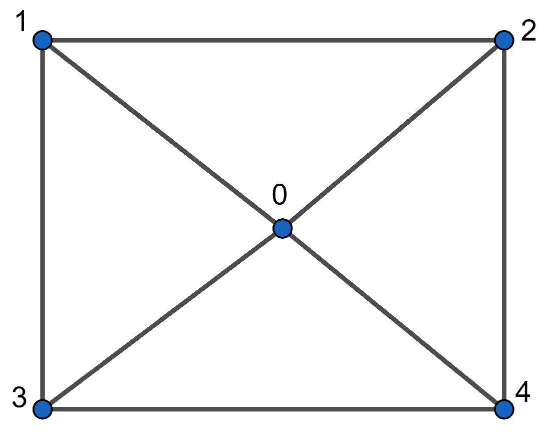
Figure 2.
The graph .
4. Laplacian Spectrum of
In this section, we explore the Laplacian spectrum of for . For , we give the weight to the vertex i of the graph . We define the integer
for . The vertex weighted Laplacian matrix of defined in Theorem 1 is given by the following:
where
for .
The next remark is an immediate result of Proposition 2.4 in [5].
Remark 1.
The following statements hold:
- 1.
- If , then .
- 2.
- If , then
Lemma 4.
.
Proof.
The proof is direct from the definition of in Equation (4). □
The following result describes the Laplacian spectrum of .
Theorem 3.
Let . Then, we have the following:
where and indicates that is added to each element in the multiset .
Proof.
By Lemma 3, we have the following:
As a result, the outcome follows directly from Lemma 4 and Theorem 1. □
By Corollary 1, is either or for . By Theorem 3, out of the n number of Laplacian eigenvalues of , are known to be nonzero integer values. The remaining Laplacian eigenvalues of will come from the Laplacian eigenvalues of .
Corollary 2.
Let . The Laplacian spectrum of is as follows:
- 1.
- If , then we have the following:
- 2.
- If , then we have the following:
Proof.
By the above argument and Remark 1, the result holds. □
The following Theorem presents the Laplacian spectrum of for .
Theorem 4.
Let .
- 1.
- If , then the Laplacian spectrum of is
- 2.
- If , then
Proof.
- 1.
- Let , where . So, , and the set of distinct representatives of is . Thus, we have the following:By Corollary 2,By Equation (1), the Laplacian spectrum of and are as follows:Then, we have the following:By using Lemma 2, is isomorphic to and, hence, . So, by Theorem 2, we have the following:So,Thus, the Laplacian spectrum of is given by Equation (5).
- 2.
- Let , where . Note that is the vertex set of the graph . Thus, we have the following:By Corollary 2,By using Lemma 2, is isomorphic to and, hence, . So, by Theorem 2, we have the following:Hence,□
Now, we find the Laplacian spectrum of for . The following theorem can be derived using reasoning analogous to that employed in the proof of Theorem 4, and thus its proof is omitted.
Theorem 5.
Let .
- 1.
- If , then the Laplacian spectrum of is as follows:
- 2.
- If , then the Laplacian spectrum of is as follows:
Directly following from Theorem 5, the subsequent results are obtained.
Corollary 3.
) is the Laplacian integral for all n.
Corollary 4.
Let . The Laplacian spectral radius of is as follows:
Corollary 5.
Let . The algebraic connectivity of is as follows:
5. Vertex Connectivity of
In this section, we obtain the vertex connectivity of when and , where . To achieve this goal, we calculate the number of internally disjoint paths between any two nonadjacent vertices in , which allows us to be ready to explore by using Menger’s theorem.
5.1. Structure of
The subsequent result will be utilized in the upcoming analysis.
Lemma 5
([19]). Suppose . Then, the following statements hold:
- 1.
- Let . The induced subgraph of is isomorphic to ( is the cocktail party graph, which is obtained from the complete graph , , by deleting the perfect matching, where a perfect matching in a graph G is a spanning subgraph W of G, where each vertex has a degree of 1). If , then is .
- 2.
- Let and . If , then every vertex of is adjacent to vertices of .
- 3.
- Let and . If , then every vertex of is nonadjacent to any vertex of .
Now, we study the structure of , where , analogous to Section 3. In this case, we choose the maximal ideal . Let be the set of distinct representatives of . For , we denote the following:
Note that the sets form a partition of the vertex set of . Thus, we have the following:
This implies that any two vertices x and y that belong to the above union are adjacent if and only if . Let . Then, for . Let , and say . Denote by the unique element in which is a multiple of q.
Note that, Lemma 5 implies that the partition of forms an almost equitable partition. This means that every vertex in has the same number of neighbors in for and . Also, is isomorphic to and is isomorphic to , where .
Let be defined as the simple graph whose vertices are , where , so that . Two distinct vertices and in are adjacent if and only if , which is equivalent to each vertex in being adjacent to vertices in .
Example 2.
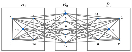
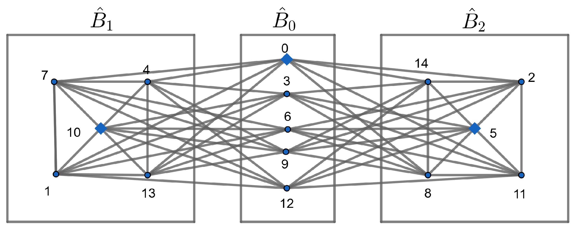
The vertex set of is the union , where , , and . From Figure 3 below, we observe the following:
Figure 3.
The graph .
- 1.
- is nonadjacent to in since .
- 2.
- Each vertex in and is adjacent to 4 vertices in .
- 3.
- is isomorphic to and and are isomorphic to . The diamond-shaped vertices 0, 5, and 10 represent in , , and , respectively. Note that these vertices are multiples of 5.
From now on, throughout the rest of this paper, when we write and , it is assumed that . This assumption ensures that the sets and are distinct. The following two results determine the neighbors and the number of common neighbors of the vertices in , which help us to calculate the number of internally disjoint paths between any two nonadjacent vertices in .
Lemma 6.
Let . If , then there are neighbors of in . On the other hand, has neighbors in .
Proof.
Suppose . For , for all except . Consequently, is adjacent to in when . Then, there are neighbors of in . If , then for all . Thus, is adjacent to all vertices in . Therefore, there are neighbors of in . □
Lemma 7.
If , then the following statements hold:
- 1.
- If and are nonadjacent in , then the number of common neighbors between and in is .
- 2.
- If and are adjacent in , where , then the number of common neighbors between and in is .
- 3.
- The number of common neighbors between and in is .
Proof.
Let .
- 1.
- Let and be nonadjacent in . By Lemma 6, and . Hence, is adjacent to all vertices in except . Similarly, is adjacent to all vertices in except . So, and are adjacent to all vertices in except and . Therefore, there are common neighbors between and in .
- 2.
- Let and be adjacent in , where . According to Lemma 6, and are nonadjacent to and in , respectively. So, and are adjacent to all vertices in except and , respectively. Then, the set of common neighbors between and in isThus, there are common neighbors between and in .
- 3.
- By Lemma 6, is adjacent to all vertices in . Also, is adjacent to all vertices in except . So, the set of common neighbors between and in isThen, there are common neighbors between and in .
□
The next result finds the number of common neighbors between nonadjacent vertices through , where is a neighbor of in .
Lemma 8.
Let be nonadjacent and be a neighbor of in . Then, x and y have common neighbors in .
Proof.
By Part 2 of Lemma 5, both x and y are adjacent to vertices in . Suppose that x and y have the same neighbors in . Then, x and y are adjacent to all vertices in except . This implies that is adjacent to vertices in , a contradiction with Part 2 of Lemma 5. Then, x and y are adjacent to all vertices in except and , respectively. So, the number of common neighbors between x and y in is . □
The following result determines the number of common neighbors between nonadjacent vertices and through , where is a common neighbor between and in .
Lemma 9.
Let and be nonadjacent and be a common neighbor between and in .
- 1.
- If x and y have the same neighbors in , then the number of common neighbors in between x and y is .
- 2.
- If x and y do not have the same neighbors in , then the number of common neighbors in between x and y is .
Proof.
Let and be nonadjacent and be a common neighbor between and in .
- 1.
- The proof is direct from Part 2 of Lemma 5.
- 2.
- Suppose x and y do not have the same neighbors in . By Part 2 of Lemma 5, both x and y have neighbors in . That is, x and y are adjacent to all vertices in except and , respectively. So, the number of the common neighbors in between x and y is .
□
The next result characterizes the nonadjacent vertices of for which the relation in Part 1 of Lemma 9 holds when is adjacent to in .
Proposition 1.
Let and be nonadjacent, be adjacent to in , and be a common neighbor between and in . Then, x and y have the same neighbors in if and only if and .
Proof.
Suppose that x and y have the same neighbors in . Then, x and y are adjacent to all vertices in except by Part 2 of Lemma 5. We assume that and . Suppose that , , and , where and . Since is adjacent to in and x is nonadjacent to y, then and , this implies that . Similarly, since is adjacent to and in , then and . So, we have the following:
So, ; this implies that 2 divides and, hence, is a multiple of q, in this case . But is adjacent to all vertices in and except and , respectively. This contradicts with and . So, and .
Assume that and . Then, x is adjacent to vertices of by Part 2 of Lemma 5, that is, x is adjacent to all vertices of except , where and . Similarly, y is adjacent to all vertices of except . Then, the result is obtained. □
5.2. Number of Internally Disjoint Paths Between Nonadjacent Vertices in
The next two results calculate the number of internally disjoint paths (IDPs) between nonadjacent vertices x and y in .
Lemma 10.
Let be nonadjacent. Then, there are IDPs of length 2 between x and y.
Proof.
If , then is isomorphic to by Part 1 of Lemma 5. Since represents , then is adjacent to all vertices in . Since x is nonadjacent to y, then neither x nor y is in . So, there are common neighbors between x and y and, hence, there are IDPs of length 2 between x and y in . Let be a neighbor of in . By Lemma 8, there are common neighbors between x and y in . Hence, there are IDPs of length 2 through . By Lemma 6, there are neighbors of in and, hence, there are IDPs of length 2 between x and y through all neighbors of in . Thus, the total number of IDPs of length 2 between x and y is as follows:
If , then is isomorphic to , by Part 1 of Lemma 5. So, there is no path between x and y in . By Lemma 8, there are common neighbors between x and y in , where is a neighbor of in . Hence, there are IDPs of length 2 through . By Lemma 6, there are neighbors of in and, hence, there are IDPs of length 2 between x and y. □
Lemma 11.
Let be nonadjacent.
- 1.
- If , then there are IDPs of length 4 between x and y.
- 2.
- If , then there are IDPs of length 4 between x and y.
Proof.
Let be nonadjacent and be a neighbor of in . By proof of Lemma 8, x and y are adjacent to all vertices of except and , respectively.
- 1.
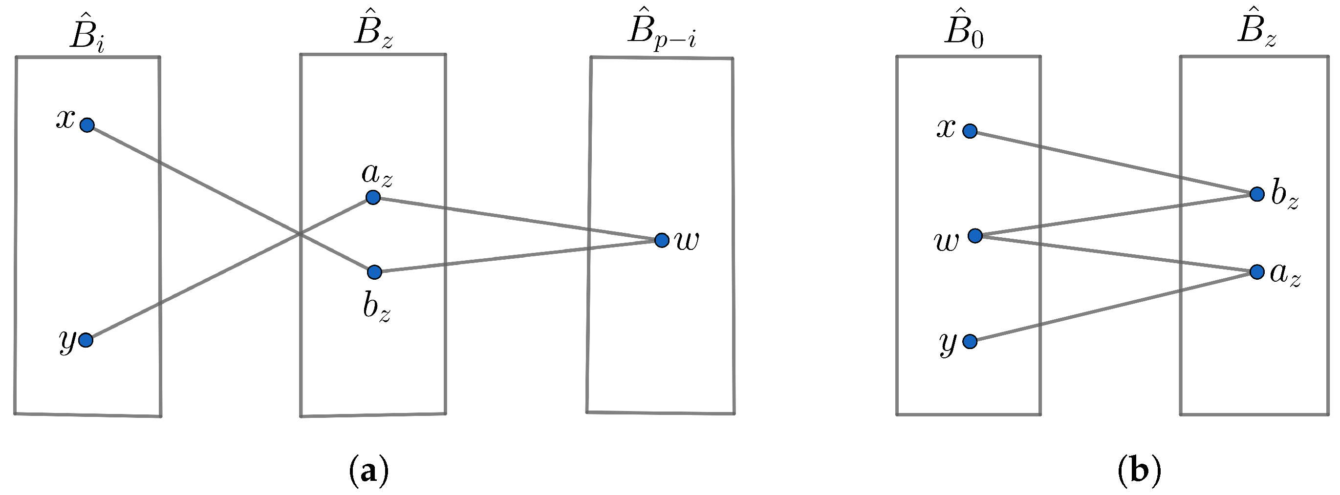
- Suppose . By Part 2 of Lemma 5, and in are adjacent to vertices of . Since we investigate the IDPs between x and y through and , we can choose a vertex w from that is adjacent to both and . This path will be of length 4, as illustrated in Figure 4a. Similarly, for each neighbor of in there is one internally disjoint path of length 4 between x and y. By Lemma 6, there are neighbors of in . Therefore, there are IDPs of length 4 between x and y through all neighbors of .
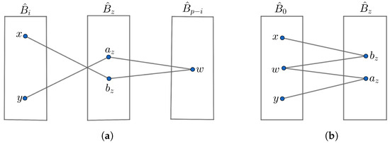 Figure 4. when . (a) when . (b) when .
 - 2.
- Suppose . By Part 2 of Lemma 5, and in are adjacent to vertices of . Following a similar approach to the proof in Part 1, we identify one internally disjoint path of length 4, illustrated in Figure 4b. By Lemma 6, the number of neighbors of in is . So, there are IDPs of length 4 between x and y through all neighbors of .
□
The next two results determine the number of IDPs between nonadjacent vertices and , where is nonadjacent to in .
Lemma 12.
Let and be nonadjacent, be nonadjacent to in , and be a common neighbor between and in .
- 1.
- If x and y have the same neighbors in , then there are IDPs of length 2 between x and y.
- 2.
- If x and y do not have the same neighbors in , then there are IDPs of length 2 between x and y.
Proof.
Let be nonadjacent to in . By Part 1 of Lemma 7, there are common neighbors between and in .
- 1.
- If x and y have the same neighbors in , then there are common neighbors between x and y in by Lemma 9. Thus, there are IDPs of length 2 between x and y through . Hence, there are IDPs of length 2 between x and y through all common neighbors between and in .
- 2.
- If x and y do not have the same neighbors in , then there are common neighbors between x and y in by Lemma 9. So, there are IDPs of length 2 between x and y through . Therefore, there are IDPs of length 2 between x and y through all common neighbors between and in .
□
Lemma 13.
Let and be nonadjacent, be nonadjacent to in , and be a common neighbor between and in .
- 1.
- If x and y have the same neighbors in , then there are IDPs of length 4 between x and y.
- 2.
- If x and y do not have the same neighbors in , then there are IDPs of length 3 between x and y.
Proof.
Let be nonadjacent to in . By Part 1 of Lemma 7, there are common neighbors between and in .
- 1.
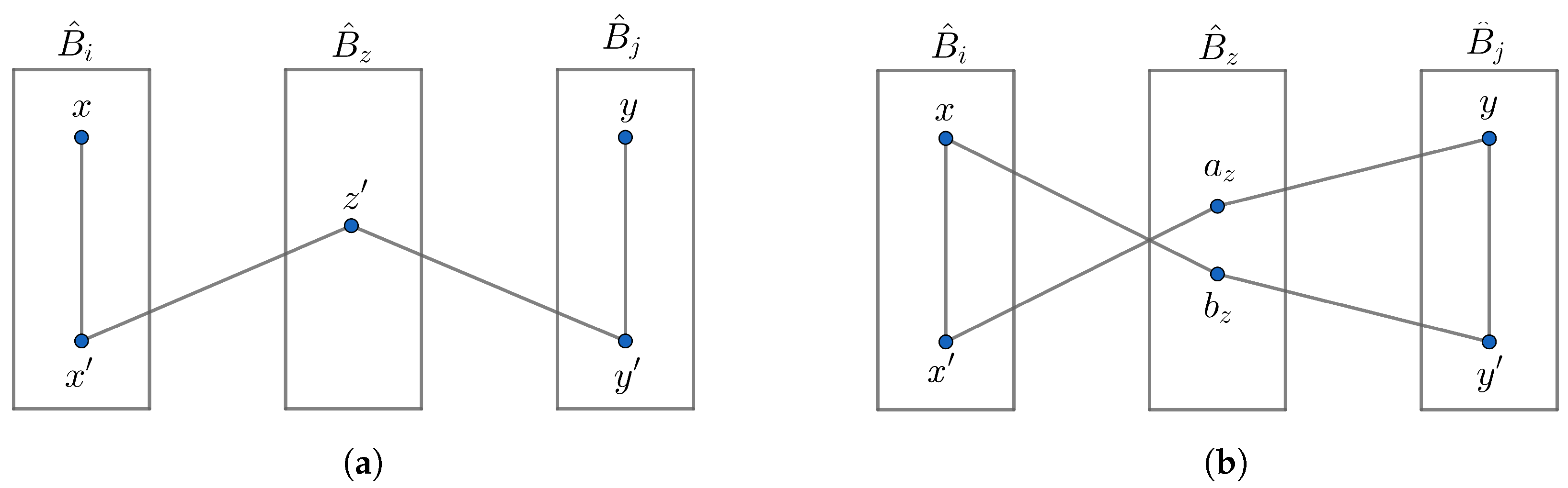
- Suppose x and y have the same neighbors in . By Lemma 5, has at least neighbors in and each of them is adjacent to vertices of . Then, we can choose a neighbor, say , of x in such that , where is nonadjacent to both x and y. Similarly, we can choose a neighbor of y in such that . Therefore, there exists a path of length 4 of the form , see Figure 5a. So, there are IDPs of length 4 between x and y through all common neighbors between and in .
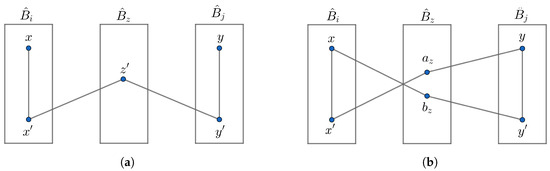 Figure 5. Paths between and , where in . (a) when x and y have the same neighbors in . (b) when x and y do not have the same neighbors in .
 - 2.
- Suppose x and y do not have the same neighbors in . By the proof of Lemma 9, x and y are adjacent to all vertices in except and , respectively. Approaching the proof similarly to Part 1, we can choose a neighbor of x in and a neighbor of y in , where and . Since and , two IDPs of length 3 exist. These paths are described in Figure 5b. Hence, there are IDPs of length 3 between x and y through all common neighbors between and in .
□
The following results find the number of IDPs between nonadjacent vertices and , where is adjacent to in .
Lemma 14.
Let and be nonadjacent and be adjacent to in . The number of IDPs of length 2 between x and y is either or .
Proof.
By Lemma 7, there are common neighbors between the adjacent vertices and , where , in and there are common neighbors between and in . Let be a common neighbor between and in . Since x and y are nonadjacent, then x and y have the following possibilities:
- 1.
- Assume that x and y have the same neighbors in . By Proposition 1 and Lemma 9, and and there are common neighbors between x and y through . So, there are IDPs of length 2 between x and y through . If , then there are IDPs of length 2 between x and y through all common neighbors between and in . Further, x (resp. y) is adjacent to all vertices in (resp. ). Also, x (resp. y) is adjacent to all vertices in (resp. ) except y (resp. x). So, the set of common neighbors between x and y in and is union . Thus, there are common neighbors between x and y in and . Consequently, there are IDPs of length 2 between x and y in and . Therefore, the total number of IDPs of length 2 between x and y is as follows:If , then there are IDPs of length 2 between x and y through all common neighbors between and in . Further, x is adjacent to all vertices in and y is nonadjacent to any vertex in . Also, x (resp. y) is adjacent to all vertices in (resp. ) except y (resp. x). So, the set of common neighbors between x and y in and are . Thus, there are common neighbors between x and y in and . Then, there are IDPs of length 2 between x and y in and . Thus, the total number of IDPs of length 2 between x and y is as follows:
- 2.
- Assume that x and y do not have the same neighbors in . By Proposition 1 and Lemma 9, and and there are common neighbors between x and y in . Thus, there are IDPs of length 2 between x and y through . If , then there are IDPs of length 2 between x and y through all common neighbors between and in . Furthermore, x (resp. y) is adjacent to all vertices except only one vertex (resp. ) in (resp. ). Also, x (resp. y) is adjacent to all vertices in (resp. ) except y (resp. x). Thus, the set of common neighbors between x and y in and is union . So, there are common neighbors between x and y in and . As a result, there are IDPs of length 2 between x and y in and . Therefore, the total number of IDPs of length 2 between x and y is as follows:If , then there are IDPs of length 2 between x and y through all common neighbors between and in . Further, x is adjacent to all vertices except only one vertex in , and y is nonadjacent to any vertex in . Also, x (resp. y) is adjacent to all vertices in (resp. ) except y (resp. x). Thus, the set of common neighbors between x and y in and is . So, there are common neighbors between x and y in and . Then, there are IDPs of length 2 between x and y in and . Thus, the total number of IDPs of length 2 between x and y is as follows:
□
Lemma 15.
Let and be nonadjacent, where is adjacent to in . The number of IDPs of length 3 between x and y is either , , or .
Proof.
We need to examine whether any -path passes through and because we are sure that (resp. ) is adjacent to (resp. ) and nonadjacent to (resp. ) in . Let be a common neighbor between and in . Since x and y are nonadjacent, then x and y have the following cases:
- 1.
- Assume that x and y have the same neighbors in . Indeed, and by Proposition 1. If , there are neighbors of x in , denote these neighbors by such that , and each of them is adjacent to vertices of by Part 2 of Lemma 5. Similarly, there are neighbors of y in , and each of them is adjacent to vertices of . To obtain the IDPs of length 3 between x and y, we choose one of the neighbors of , say , in such that is a neighbor of y. Indeed, for each in there is one internally disjoint path between x and y through and . Therefore, the total number of IDPs of length 3 between x and y through and together is equal to the number of neighbors of x in , which is . Now suppose . There are neighbors of x in and each of them is adjacent to vertices of . Since there are neighbors of y in , so there are more than paths of length 3 between x and y through and together. By applying the same method in the case where , there are IDPs of length 3 between x and y.
- 2.
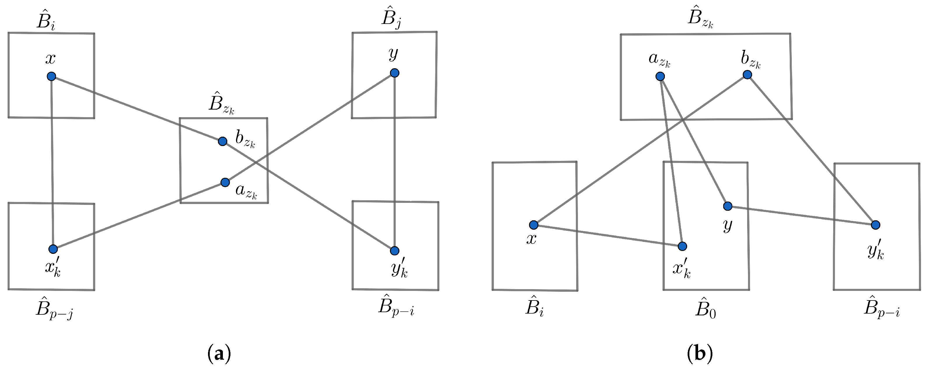
- Assume that x and y do not have the same neighbors in . So, and by Proposition 1. Suppose that is a common neighbor between and in . By the proof of Lemma 9, x and y are adjacent to all vertices in except and , respectively. Suppose . Since x has neighbors in and each of these neighbors is adjacent to vertices of , then we can choose a neighbor of x in such that . Similarly, we can choose a neighbor of y in such that . Since and , there exist two IDPs of length 3 between x and y, as illustrated in Figure 6a. By Part 2 of Lemma 7, there are common neighbors between and in . Then, there are IDPs of length 3 between x and y through all common neighbors between and in . After removing all and from and , respectively, then the number of remaining neighbors of x and y in and , respectively, is . So, there are IDPs of length 3 between x and y that pass through the remaining neighbors of x and y in and , respectively. So, the total number of IDPs of length 3 between x and y is
 Figure 6. and when and , where in . (a) and when . (b) and when .Suppose . Since x has neighbors in and each of these neighbors is adjacent to vertices of , then we can choose a neighbor of x in such that . Similarly, we can choose a neighbor of y in such that . Since and , there exist two internally disjoint paths of length 3 between x and y, as illustrated in Figure 6b. By Part 3 of Lemma 7, there are common neighbors between and in . Consequently, there are IDPs of length 3 between x and y through all common neighbors between and in . After removing all and from and , respectively, then the number of remaining neighbors of x and y in and , respectively, is . So, there are IDPs of length 3 between x and y that pass through the rest of the neighbors of x and y in and , respectively, together. So, the total number of IDPs of length 3 between x and y is as follows:
□
5.3. Vertex Connectivity of
The next result is of crucial importance to our study in this section.
Theorem 6.
Suppose are distinct primes. The vertex connectivity of is as follows:
Proof.
Let x and y be nonadjacent in . In this proof, we will calculate the maximum number of IDPs between any two nonadjacent vertices. There are several cases for x and y, as follows:
Case 1: Suppose . By Lemma 10, there are IDPs of length 2 between x and y. In addition, there are other IDPs depending on the following cases for i:
(a) Suppose . By Lemma 11, there are IDPs of length 4 between x and y. So,
(b) Suppose . By Lemma 11, there are IDPs of length 4 between x and y. So,
Case 2: Let and , where is nonadjacent to in . Let be a common neighbor between and in . The following cases arise for x and y:
(a) If y has the same neighbors as x in , then there are IDPs of length 2 between x and y by Lemma 12. According to Lemma 13, there are IDPs of length 4 between x and y. Hence,
(b) If x and y do not have the same neighbors in , there are IDPs of length 2 between x and y by Lemma 12. According to Lemma 13, there are IDPs of length 3 between x and y. Hence,
Case 3: Let and , where is adjacent to in . Let be a common neighbor between and in . There are the following cases for x and y:
(a) If y has the same neighbors as x in , then there are IDPs of length 2 between x and y by the proof of Lemma 14. According to the proof of Lemma 15, there are IDPs of length 3 between x and y. Hence,
(b) If x and y do not have the same neighbors in , then there are IDPs of length 2 between x and y by the proof of Lemma 14. In addition, there are other IDPs, depending on the following cases for i and j:
(1) Suppose . According to the proof of Lemma 15, there are IDPs of length 3 between x and y. Therefore,
(2) Suppose . According to the proof of Lemma 15, there are IDPs of length 3 between x and y. So,
From the above cases and by Menger’s theorem, we have the following:
□
Now, let us explore the vertex connectivity of where , with and at least one of r or s must be greater than 1.
Theorem 7.
Let , where . Then, the vertex connectivity of is
Proof.
By Lemma 3, the unit graph is
According to Lemma 2, is isomorphic to . Hence, by Theorem 6, we obtain the following:
Note that, for every vertex i of , we have vertices in . Since for , then we have the following:
□
6. Conclusions and Conjectures
In this paper, we investigated the structure of and its associated properties. We determined the Laplacian spectrum and vertex connectivity of for various values of n, providing detailed proofs and utilizing the structure of for . Specifically, we showed that can be expressed as a generalized join graph. We established that is the Laplacian integral, deduced its algebraic connectivity, and identified its Laplacian spectral radius. Using Menger’s theorem and the graph structure, we determined the vertex connectivity of and . The results presented in this paper have been rigorously verified through Python 3.12 programming, as detailed in Appendix A.
Based on the results for the vertex connectivity of in Theorems 6 and 7 and on some actual experimental data (as with the Python verifications), we present the following conjectures:
- Conjecture I: Let , where . Then,
- Conjecture II: Let , where . Then,
These conjectures provide a foundation for future exploration of the vertex connectivity of for larger values of n and may lead to further generalizations in algebraic graph theory.
Author Contributions
Investigation, A.A. and W.F.; Methodology, A.A. and W.F.; Writing—original draft preparation, A.A., W.F. and H.A.; Writing—review and editing, A.A., W.F. and H.A.; supervision, W.F. and H.A. All authors have read and agreed to the published version of the manuscript.
Funding
This research received no external funding.
Data Availability Statement
All data are included within this article.
Conflicts of Interest
The authors confirm that there are no conflicts of interest associated with this work.
Appendix A
Pranjali et al. [20] provided the generation code of the unit graph of . We utilized this code in Python programming to create the following algorithm, which verifies the validity of our results:
| Algorithm A1 Unit Graph Generation and Analysis |
Input:
|
References
- Grimaldi, R.P. Graphs from rings. In Proceedings of the 20th Southeastern Conference on Combinatorics, Graph Theory, and Computing, Boca Raton, FL, USA, 20–24 February 1989; Volume 71, pp. 95–103. [Google Scholar]
- Su, H.; Yang, L. Domination number of unit graph of . Discrete Math. Algorithms Appl. 2020, 12, 2050059. [Google Scholar] [CrossRef]
- Shen, S.; Liu, W.; Jin, W. Laplacian eigenvalues of the unit graph of the ring . Appl. Math. Comput. 2023, 459, 128268. [Google Scholar] [CrossRef]
- Fakieh, W.; Alsaluli, A.; Alashwali, H. Laplacian spectrum of the unit graph associated to the ring of integers modulo pq. AIMS Math. 2024, 9, 4098–4108. [Google Scholar] [CrossRef]
- Ashrafi, N.; Maimani, H.R.; Pournaki, M.R.; Yassemi, S. Unit graphs associated with rings. Commun. Algebra 2010, 38, 2851–2871. [Google Scholar] [CrossRef]
- Maimani, H.R.; Pournaki, M.R.; Yassemi, S. Necessary and sufficient conditions for unit graphs to be Hamiltonian. Pac. J. Math. 2011, 249, 419–429. [Google Scholar] [CrossRef]
- Su, H.; Zhou, Y. On the girth of the unit graph of a ring. J. Algebra Appl. 2014, 13, 1350082. [Google Scholar] [CrossRef]
- Akbari, S.; Estaji, E.; Khorsandi, M.R. On the unit graph of a noncommutative ring. Algebra Colloq. 2015, 22, 817–822. [Google Scholar] [CrossRef]
- Abdelkarim, H.A.; Rawshdeh, E.; Rawashdeh, E. The eigensharp property for unit graphs associated with some finite rings. Axioms 2022, 11, 349. [Google Scholar] [CrossRef]
- Chattopadhyay, S.; Patra, K.L.; Sahoo, B.K. Laplacian eigenvalues of the zero divisor graph of the ring . Linear Algebra Appl. 2020, 584, 267–286. [Google Scholar] [CrossRef]
- Banerjee, S. Laplacian spectrum of comaximal graph of the ring . Spec. Matrices 2022, 10, 285–298. [Google Scholar] [CrossRef]
- Mathil, P.; Baloda, B.; Kumar, J. On the cozero-divisor graphs associated to rings. AKCE Int. J. Graphs Comb. 2022, 19, 238–248. [Google Scholar] [CrossRef]
- Cvetković, D.M.; Rowlison, P.; Simić, S. An Introduction to the Theory of Graph Spectra; London Mathematical Society Student Texts 75; Cambridge University Press, Inc.: Cambridge, UK, 2010. [Google Scholar] [CrossRef]
- Pirzada, S.; Ganie, H.A. On the Laplacian eigenvalues of a graph and Laplacian energy. Linear Algebra Appl. 2015, 486, 454–468. [Google Scholar] [CrossRef]
- Schwenk, A.J. Computing the characteristic polynomial of a graph. In Proceedings of the Capital Conference, Graphs and Combinatorics, Lecture Notes in Mathematics, Washington, DC, USA, 18–22 June 1973; Springer: Berlin/Heidelberg, Germany, 1973; Volume 406, pp. 153–172. [Google Scholar] [CrossRef]
- Cardoso, D.M.; De Freitas, M.A.A.; Martins, E.A.; Robbiano, M. Spectra of graphs obtained by a generalization of the join of graph operation. Discrete Math. 2013, 313, 733–741. [Google Scholar] [CrossRef]
- Fiedler, M. Algebraic connectivity of graphs. Czechoslovak Math. J. 1973, 23, 298–305. [Google Scholar] [CrossRef]
- Balakrishnan, R.; Ranganathan, K. A Textbook of Graph Theory; Springer: New York, NY, USA, 2000. [Google Scholar]
- Alsaluli, A.; Fakieh, W.; Alashwali, H. Laplacian spectrum of the unit graph of the ring . In Proceedings of the International Conference and Exhibition for Science (ICES 2023), College of Science, King Saud University, Riyadh, Saudi Arabia, 6–8 February 2023. [Google Scholar]
- Pranjali; Acharya, M. Energy and Wiener index of unit graph. Appl. Math. Inf. Sci. 2015, 9, 1339–1343. [Google Scholar]
Disclaimer/Publisher’s Note: The statements, opinions and data contained in all publications are solely those of the individual author(s) and contributor(s) and not of MDPI and/or the editor(s). MDPI and/or the editor(s) disclaim responsibility for any injury to people or property resulting from any ideas, methods, instructions or products referred to in the content. |
© 2024 by the authors. Licensee MDPI, Basel, Switzerland. This article is an open access article distributed under the terms and conditions of the Creative Commons Attribution (CC BY) license (https://creativecommons.org/licenses/by/4.0/).