Geometric Nature of the Turánian of Modified Bessel Function of the First Kind

Abstract

This work explores the geometric properties of the Turanian of the modified Bessel function of the first kind (TMBF). Using the properties of the digamma function, we establish conditions under which the normalized TMBF satisfies starlikeness, convexity, k-starlikeness, k-uniform convexity, pre-starlikeness, lemniscate starlikeness, and convexity, and under which exponential starlikeness and convexity are obtained. By combining methods from complex analysis, inequalities, and functional analysis, the article advances the theory of Bessel functions and hypergeometric functions. The established results could be useful in approximation theory and bounding the behavior of functions.

1. Introduction

Bessel functions hold significant importance across multiple domains, including mathematical physics and engineering, quantum mechanics, signal processing, fluid dynamics, electromagnetism, acoustics, and heat conduction. Specifically, the Bessel functions appear everywhere in problems admitting cylindrical symmetry, such as pipes, tubes, cylindrical wave guides, beams, etc. In [1], Baricz et al. introduced conditions for normalized Bessel function to exhibit convexity and starlikeness within the unit disk, resolving an open problem and presenting a novel inequality for the Euler $\Gamma$ function. Sufficient conditions for the univalence of the generalized Bessel functions in the unit disk are established by Prajapat in [2]. In [3], Mondal and Swaminathan explored the geometric properties of generalized Bessel functions, yielding various conditions for close-to-convexity, starlikeness, and convexity. Conditions for close-to-convexity of some special functions, including the Bessel functions, are deduced by Baricz and Szasin [4], utilizing results on transcendental entire functions and Pólya’s Theorem. In [5], Aktas et al. obtained tight bounds for the radii of starlikeness of normalized Bessel, Struve, and Lommel functions of the first kind. The geometric properties of generalized Struve functions were derived by Sarkar, Das, and Mondal in their work [6]. Aktas, Baricz, and Singh explored various geometric properties of normalized hyper-Bessel functions in [7]. In [8,9], they obtained tight lower and upper bounds for the radii of starlikeness and convexity of Jackson’s second and third q-Bessel functions, respectively. Additionally, Zayed and Bulboaca studied the normalization of generalized Bessel functions in [10], establishing sufficient conditions for their starlikeness, convexity, and close-to-convexity in the open unit disk. Furthermore, in [11], Mehrez, Das, and Kumar examined some geometric properties of products of modified Bessel functions, including starlikeness, convexity, and close-to-convexity.

The modified Bessel function of the first kind, denoted as $I_{\nu }\left(z\right)$ [12], is a special function satisfying the differential equation:

$$z^2{\displaystyle \frac{d^{2}y}{d{z}^2}}+z{\displaystyle \frac{dy}{dz}}-(z^2+{\nu }^2)y=0,$$

where $\nu$ is a real parameter. It can also be expressed through its infinite series representation:

$$I_{\nu }\left(z\right)={\left({\displaystyle \frac{z}{2}}\right)}^{\nu }\sum _{k=0}^{\infty }{\displaystyle \frac{1}{k!\Gamma (k+\nu +1)}}{\left({\displaystyle \frac{z}{2}}\right)}^{2k}.$$

Furthermore, the Bessel I and J functions are closely related to the generalized hypergeometric (GHG) functions.

$${}_{p}F_q(a_1,\dots ,a_p;b_1,\dots ,b_q;x)=\sum _{m=0}^{+\infty }{\displaystyle \frac{x^m}{\Gamma (m+1)}}\prod _{k=1}^p{\displaystyle \frac{\Gamma (a_k+m)}{\Gamma \left(a_k\right)}}\prod _{k=1}^q{\displaystyle \frac{\Gamma \left(b_k\right)}{\Gamma (b_k+m)}}=\sum _{r=0}^{+\infty }{\displaystyle \frac{x^r}{r!}}{\displaystyle \frac{{\prod }_{j=0}^{p-1}{\left(a_j\right)}_r}{{\prod }_{j=0}^{q-1}{\left(b_j\right)}_r}},$$

(1)

where ${\left(a\right)}_r$ and ${\left(b\right)}_r$ denote rising factorials and ${\left(a\right)}_0=1$. In particular,

$$I_{\nu }\left(z\right)={\left({\displaystyle \frac{z}{2}}\right)}^{\nu }{\displaystyle \frac{1}{\Gamma (\nu +1)}}{}_{0}F_1\left(-;\nu +1;{\displaystyle \frac{z^2}{4}}\right).$$

Since Szegö’s work on the Turán inequality for classical Legendre polynomials in 1948 [13], numerous authors have extended similar results to classical orthogonal polynomials and special functions. Turán-type inequalities have seen successful applications in information theory, economic theory, and biophysics. For $\nu >-{\displaystyle \frac{1}{2}}$ series representation of the Turánian of $I_{\nu }\left(z\right)$ (see [14], Theorem 5) is given by

$${\Delta }_{\nu }\left(z\right)=I_{\nu }^2\left(z\right)-I_{\nu -1}\left(z\right)I_{\nu +1}\left(z\right)={\displaystyle \frac{1}{\sqrt{\pi }}}\sum _{m=0}^{\infty }{\displaystyle \frac{\Gamma (\nu +m+\frac{1}{2})z^{2\nu +2m}}{m!\Gamma (\nu +m+2)\Gamma (2\nu +m+1)}}.$$

(2)

From the above presentation we see that the series in Equation (2) can be represented by a GHG function as

$${\Delta }_{\nu }\left(z\right)={\displaystyle \frac{z^{2\nu }}{\sqrt{\pi }}}{\displaystyle \frac{\Gamma (\nu +\frac{1}{2})}{\Gamma (\nu +2)\Gamma (2\nu +1)}}{}_{1}F_2\left(\nu +{\displaystyle \frac{1}{2}};\nu +2,2\nu +1;z^2\right)$$

(3)

Let ${\mathbb{D}}_r=\{z\in \mathbb{C}:|z|<r\}$, where $r>0$ and ${\mathbb{D}}_1=\mathbb{D}$. We consider the class $\mathcal{A}$ containing the analytic functions f defined on ${\mathbb{D}}_r$ and satisfying $f\left(0\right)=f^{\prime }\left(0\right)-1=0$. A function $f\in \mathcal{A}$ is considered starlike in the disk ${\mathbb{D}}_r$ if it is univalent and its image forms a starlike domain centered around the origin [15]. Analytically,

$${\displaystyle f\in \mathcal{A} \mathrm{is} \mathrm{starlike} \mathrm{in} {\mathbb{D}}_r\iff \Re \left(\frac{\zeta f^{\prime }\left(\zeta \right)}{f\left(\zeta \right)}\right)>0 \mathrm{for} \zeta \in {\mathbb{D}}_r.}$$

Moreover,

$${\displaystyle f\in \mathcal{A} \mathrm{is} \mathrm{starlike} \mathrm{of} \mathrm{order} \delta \iff \Re \left(\frac{\zeta f^{\prime }\left(\zeta \right)}{f\left(\zeta \right)}\right)>\delta \mathrm{for} \zeta \in {\mathbb{D}}_r,}$$

where $0\le \delta <1$. The class of starlike functions of order $\delta$ in $\mathbb{D}$, denoted by $\mathcal{ST}\left(\delta \right)$, simplifies to $\mathcal{ST}$ when $\delta =0$.

Also, a function $f\in \mathcal{A}$ is convex in ${\mathbb{D}}_r$ if it is univalent in ${\mathbb{D}}_r$ and its image $f\left({\mathbb{D}}_r\right)$ is a convex domain [15].

Analytically,

$${\displaystyle f\in \mathcal{A} \mathrm{is} \mathrm{convex} \mathrm{in} {\mathbb{D}}_r\iff \Re \left(1+\frac{\zeta f^{″}\left(\zeta \right)}{f^{\prime }\left(\zeta \right)}\right)>0 \mathrm{for} \zeta \in {\mathbb{D}}_r.}$$

Moreover,

$${\displaystyle f\in \mathcal{A} \mathrm{is} \mathrm{convex} \mathrm{of} \mathrm{order} \delta \iff \Re \left(1+\frac{\zeta f^{″}\left(\zeta \right)}{f^{\prime }\left(\zeta \right)}\right)>\delta \mathrm{for} \zeta \in {\mathbb{D}}_r,}$$

where $0\le \delta <1$.

The collection of convex functions of order $\delta$ in $\mathbb{D}$, denoted by $\mathcal{CV}\left(\delta \right)$, simplifies to $\mathcal{CV}$ when $\delta =0$.

Kanas and Wiśniowska [16] defined k-uniformly convex functions as functions $f\in \mathcal{A}$ that map circular arcs in $\mathbb{D}$ centered at points $\omega$ with $\left|\omega \right|\le k$ to convex curves. They also provided a one-variable characterization for this class. Let $f\in \mathcal{A}$ and $0\le k<\infty$ then

$$f\in \mathcal{A} \mathrm{is} k\text{-uniformly} \mathrm{convex} \iff \Re \left(1+{\displaystyle \frac{\zeta f^{\prime \prime }\left(\zeta \right)}{f^{\prime }\left(\zeta \right)}}\right)>k\left|{\displaystyle \frac{\zeta f^{\prime \prime }\left(\zeta \right)}{f^{\prime }\left(\zeta \right)}}\right|, \mathrm{for} \zeta \in \mathbb{D}.$$

According to [17], $1\text{-}\mathcal{UCV}=\mathcal{UCV}$ and $0\text{-}\mathcal{UCV}=\mathcal{CV}$.

A similar class, $k\text{-}\mathcal{ST}$, related to starlike functions, was also defined by Kanas and Wi’sniowska in [18] known as k starlike functions.

$$f\in \mathcal{A} \mathrm{is} k\text{-starlike}\iff \Re \left({\displaystyle \frac{\zeta f^{\prime }\left(\zeta \right)}{f\left(\zeta \right)}}\right)>k\left|{\displaystyle \frac{\zeta f^{\prime }\left(\zeta \right)}{f\left(\zeta \right)}}-1\right|, \mathrm{for} \zeta \in \mathbb{D}.$$

When $k=0$, the class $k\text{-}\mathcal{ST}$ reduces to the well-known class of starlike functions, $\mathcal{ST}$. For $k=1$, the class $1\text{-}\mathcal{ST}$ is identical to the class ${\mathcal{S}}_p$, introduced by Rønning [19]. Geometrically, a function $f\in k\text{-}\mathcal{ST}$, ($k\text{-}\mathcal{UCV}$) if the image of $\mathbb{D}$ under the mapping ${\mathcal{SQ}}_f\left(\zeta \right)={\displaystyle \frac{\zeta f^{\prime }\left(\zeta \right)}{f\left(\zeta \right)}}$, $\left({\mathcal{CQ}}_f\left(\zeta \right)=1+{\displaystyle \frac{\zeta f^{\prime \prime }\left(\zeta \right)}{f^{\prime }\left(\zeta \right)}}\right)$ is contained within the conic region ${\Omega }_k$. This domain ${\Omega }_k$ is defined by the condition $1\in {\Omega }_k$ and is bounded by the curve

$$\partial {\Omega }_k=\{\omega =x+iy\in \mathbb{C}:x^2=k^2{(x-1)}^2+k^2{y}^2\},0\le k<\infty .$$

Several renowned subclasses of starlike and convex functions associated with various domains that exhibit symmetry across the real axis include lemniscate starlike functions and exponential starlike functions. Lemniscate starlike functions, introduced by Sokól and Stankiewicz [20], are characterized by the image of the unit disk under the mapping ${\mathcal{SQ}}_f\left(\zeta \right)$ being contained within the region bounded by the right half of the Bernoulli lemniscate $L=\{\omega \in \mathbb{C}:\Re \left(\omega \right)>0,|{\omega }^2-1|=1\}$. Similarly, $f\in \mathcal{A}$ is lemniscate convex if ${\mathcal{CQ}}_f\left(\mathbb{D}\right)$ contained inside L. The classes ${\mathcal{S}}_L^{\ast }$ and ${\mathcal{C}}_L$ denote the lemniscate starlike and lemniscate convex functions, respectively. The starlike and convex functions associated with the exponential function, introduced by Mendiratta et al. [21] are denoted by ${\mathcal{S}}_e^{\ast }$ and ${\mathcal{C}}_e$, respectively. These classes are defined as follows:

$${\mathcal{S}}_e^{\ast }=\left\{f\in \mathcal{A}:{\mathcal{SQ}}_f\left(\mathbb{D}\right)\subset \mathcal{E}\right\}and{\mathcal{C}}_e=\left\{f\in \mathcal{A}:{\mathcal{CQ}}_f\left(\mathbb{D}\right)\subset \mathcal{E}\right\},$$

where $\mathcal{E}=\left\{exp\left(\zeta \right):\zeta \in \mathbb{D}\right\}$.

Here, we will establish various geometrical properties of the TMBF. To achieve this, we adopt the following normalization approach.

$$\begin{array}{cc}\hfill {\mathcal{T}}_{\nu }\left(z\right)& ={\displaystyle \frac{\sqrt{\pi }\Gamma (\nu +2)\Gamma (2\nu +1)}{\Gamma (\nu +\frac{1}{2})}}{z}^{1-2\nu }{\Delta }_{\nu }\left(z\right)=z+{\displaystyle \sum _{m=2}^{\infty }}q(\nu ,m)z^m,\hfill \end{array}$$

(4)

where

$$q(\nu ,m)=\left\{\begin{array}{cc}{\displaystyle \frac{\Gamma (\nu +2)\Gamma (2\nu +1)\Gamma (\nu +\frac{1}{2}+n)}{\Gamma (\nu +\frac{1}{2})\Gamma (\nu +2+n)\Gamma (2\nu +1+n)n!},}\hfill & \mathrm{if}m=2n+1,n\in \mathbb{N}\hfill \\ \\ 0,\hfill & \mathrm{if}m=2n,n\in \mathbb{N}.\hfill \end{array}\right.$$

Outline

The subsequent sections of this paper are structured as follows. The paper presents the Lemmas utilized to support its main findings in Section 2. Section 3 elaborates on results concerning starlikeness of order $\alpha$, k-starlikeness, and starlikeness on ${\mathbb{D}}_{\frac{1}{2}}$, accompanied by conditions for lemniscate and exponential starlikeness of the function ${\mathcal{T}}_{\nu }\left(z\right)$. In Section 4, the analysis extends to the derivation of conditions for ${\mathcal{T}}_{\nu }\left(z\right)$, encompassing convexity of order $\alpha$, k-uniform convexity, convexity on ${\mathbb{D}}_{\frac{1}{2}}$, as well as conditions for lemniscate and exponential convexity of the function ${\mathcal{T}}_{\nu }\left(z\right)$. Concluding remarks are provided in Section 5.

2. Lemmas

The following lemmas will be used to prove the main results.

Lemma 1 

([22]). Let $f\in \mathcal{A}$ and ${\displaystyle \left|\frac{f\left(z\right)}{z}-1\right|<1}$ for each $z\in \mathbb{D}$, then f is univalent and starlike in ${\mathbb{D}}_{\frac{1}{2}}$.

Lemma 2 

([23]). Let $f\in \mathcal{A}$ and ${\displaystyle \left|f^{\prime }\left(z\right)-1\right|<1}$ for each $z\in \mathbb{D}$, then f is convex in ${\mathbb{D}}_{\frac{1}{2}}$.

Lemma 3 

([21], Lemma 2.2). The exponential function $\mathcal{E}\left(z\right)$, satisfies

$$\underset{\theta \in [-\pi ,\pi ]}{min}\left\{\left|\mathcal{E}\left(e^{i\theta }\right)-1\right|\right\}=1-{\displaystyle \frac{1}{e}}.$$

Lemma 4 

([18]). Assume that $f\in \mathcal{A}$ with ${\displaystyle f\left(z\right)=z+\sum _{n=2}^{\infty }{a}_n{z}^n}$. If

$${\displaystyle \sum _{n=2}^{\infty }\left(n+k(n-1)\right)\left|a_n\right|<1, for some 0\le k<\infty ,}$$

then $f\in k\text{-}\mathcal{ST}$.

Lemma 5 

([16]). Let $0\le k<\infty$ and $f\in \mathcal{A}$ with ${\displaystyle f\left(z\right)=z+\sum _{n=2}^{\infty }{a}_n{z}^n}$. If

$${\displaystyle \sum _{n=2}^{\infty }(n-1)n\left|a_n\right|<\frac{1}{k+2},}$$

then $f\in k\text{-}\mathcal{UCV}$.

Lemma 6 

([24]). Let $t>1$, then the following inequality for the digamma function $\psi \left(t\right)={\displaystyle \frac{{\Gamma }^{\prime }\left(t\right)}{\Gamma \left(t\right)}}$ holds:

$$log\left(t\right)-\gamma \le \psi \left(t\right)\le log\left(t\right)$$

where γ denotes the Euler–Mascheroni constant.

3. Starlikeness of ${\mathcal{T}}_{\nu }$

This section investigates several properties of starlikeness for ${\mathcal{T}}_{\nu }$. We establish criteria for the starlikeness of order $\delta$ of ${\mathcal{T}}_{\nu }\left(z\right)$ and present several corollaries and examples for particular instances.

Theorem 1. 

Assume that $\nu >-{\displaystyle \frac{1}{2}}$. Suppose that the following criteria are satisfied:

(i) 

$e^{2\gamma }(\nu +{\displaystyle \frac{3}{2}})\le 2(\nu +3)(\nu +1)$

(ii) 

$\nu +2\ge {\displaystyle \frac{e}{1-\delta }}+{\displaystyle \frac{(e-1)}{2}}$

then ${\mathcal{T}}_{\nu }$ is a starlike function of order δ in $\mathbb{D}$.

Proof. 

To prove the desired result, it is enough to show that

$$\left|{\displaystyle \frac{z{{\mathcal{T}}_{\nu }}^{\prime }\left(z\right)}{{\mathcal{T}}_{\nu }\left(z\right)}-1}\right|=\left|{\displaystyle \frac{{\displaystyle {{\mathcal{T}}_{\nu }}^{\prime }\left(z\right)-\frac{{\mathcal{T}}_{\nu }\left(z\right)}{z}}}{{\displaystyle \frac{{\mathcal{T}}_{\nu }\left(z\right)}{z}}}}\right|<1-\delta ,(\forall z\in \mathbb{D}).$$

Now, from (4), we have

$$\begin{array}{cc}\hfill \left|{\displaystyle {{\mathcal{T}}_{\nu }}^{\prime }\left(z\right)-\frac{{\mathcal{T}}_{\nu }\left(z\right)}{z}}\right|& ={\displaystyle \frac{\Gamma (\nu +2)\Gamma (2\nu +1)}{\Gamma (\nu +\frac{1}{2})}}\left|{\displaystyle {\displaystyle \sum _{n=1}^{\infty }}\frac{2n\Gamma \left(\nu +\frac{1}{2}+n\right)z^{2n}}{\Gamma (\nu +2+n)\Gamma \left(2\nu +1+n\right)n!}}\right|\hfill \\ \hfill & <{\displaystyle \frac{2\Gamma (\nu +2)\Gamma (2\nu +1)}{\Gamma (\nu +\frac{1}{2})}}{\displaystyle \sum _{n=1}^{\infty }}a(\nu ,n){\displaystyle \frac{1}{(n-1)!}},(\forall z\in \mathbb{D}),\hfill \end{array}$$

(5)

where

$${\displaystyle a(\nu ,n)=\frac{\Gamma \left(\nu +\frac{1}{2}+n\right)}{\Gamma (\nu +2+n)\Gamma \left(2\nu +1+n\right)},n\in \mathbb{N}.}$$

(6)

Now consider the function $A_1\left(s\right)$ as:

$${\displaystyle A_1\left(s\right):=\frac{\Gamma \left(\nu +\frac{1}{2}+s\right)}{\Gamma (\nu +2+s)\Gamma \left(2\nu +1+s\right)},s\in [1,\infty ).}$$

(7)

Therefore,

$$A_1^{\prime }\left(s\right)=A_1\left(s\right)A_2\left(s\right),$$

(8)

where $A_2$ is given by

$$A_2\left(s\right)=\psi \left(\nu +{\displaystyle \frac{1}{2}}+s\right)-\psi \left(\nu +2+s\right)-\psi \left(2\nu +1+s\right),s\in [1,\infty ).$$

(9)

From Lemma 6, we obtain

$$A_2\left(s\right)\le log\left(\nu +{\displaystyle \frac{1}{2}}+s\right)+2\gamma -log\left(\nu +2+s\right)-log\left(2\nu +1+s\right)=A_3\left(s\right),s\in [1,\infty ).$$

which leads to

$$\begin{array}{cc}\hfill A_3^{\prime }\left(s\right)& ={\displaystyle \frac{1}{\nu +\frac{1}{2}+s}}-{\displaystyle \frac{1}{\nu +2+s}}-{\displaystyle \frac{1}{2\nu +1+s}}\hfill \\ \hfill & ={\displaystyle \frac{(1+\nu )-2({\nu }^2+(2\nu +1)s+s^2)}{(2\nu +1+2s)(\nu +2+s)(2\nu +1+s)}}<0,s\in [1,\infty ).\hfill \end{array}$$

Since $A_3\left(s\right)$ is decreasing on $[1,\infty )$ and $A_3\left(1\right)<0$, we have $A_1^{\prime }\left(s\right)<0$ for $s\in [1,\infty )$. This implies that ${\left\{a(\nu ,n)\right\}}_{n\ge 1}$ is a decreasing. Now from Equation (5), we have

$$\begin{array}{cc}\hfill \left|{\displaystyle {{\mathcal{T}}_{\nu }}^{\prime }\left(z\right)-\frac{{\mathcal{T}}_{\nu }\left(z\right)}{z}}\right|& <{\displaystyle \frac{2\Gamma (\nu +2)\Gamma (2\nu +1)}{\Gamma (\nu +\frac{1}{2})}}{\displaystyle \sum _{n=1}^{\infty }}a(\nu ,1){\displaystyle \frac{1}{(n-1)!}},(\forall z\in \mathbb{D}).\hfill \\ \hfill & ={\displaystyle \frac{2\Gamma (\nu +2)\Gamma (2\nu +1)}{\Gamma (\nu +\frac{1}{2})}}\times {\displaystyle \frac{\Gamma \left(\nu +\frac{3}{2}\right)}{\Gamma (\nu +3)\Gamma \left(2\nu +2\right)}}{\displaystyle \sum _{n=1}^{\infty }}{\displaystyle \frac{1}{(n-1)!}}\hfill \\ \hfill & ={\displaystyle \frac{e}{(\nu +2)}}.\hfill \end{array}$$

(10)

Also,

$$\begin{array}{cc}\hfill {\displaystyle \left|\frac{{\mathcal{T}}_{\nu }\left(z\right)}{z}\right|}& {\displaystyle \ge 1-\frac{\Gamma (\nu +2)\Gamma (2\nu +1)}{\Gamma \left(\nu +\frac{1}{2}\right)}\sum _{n=1}^{\infty }a(\nu ,n)\frac{1}{n!}>1-\frac{(e-1)}{2(\nu +2)},(\forall z\in \mathbb{D}).}\hfill \end{array}$$

(11)

Combining Equations (10) and (11), we obtain

$$\begin{array}{c}\hfill {\displaystyle \left|{\displaystyle \frac{{\displaystyle {\mathcal{T}}^{\prime }\left(z\right)-\frac{\mathcal{T}\left(z\right)}{z}}}{{\displaystyle \frac{\mathcal{T}\left(z\right)}{z}}}}\right|<\frac{2e}{2(\nu +2)-(e-1)}.}\end{array}$$

(12)

From the condition (ii) it follows that

$${\displaystyle \frac{2e}{2(\nu +2)-(e-1)}\le 1-\delta .}$$

□

Corollary 1. 

Assume that $\nu >-{\displaystyle \frac{1}{2}}$. If the following conditions are satisfied:

(i) 

$e^{2\gamma }(\nu +{\displaystyle \frac{3}{2}})\le 2(\nu +3)(\nu +1)$

(ii) 

$\nu \ge e+{\displaystyle \frac{(e-1)}{2}}-2$

then ${\mathcal{T}}_{\nu }$ is a starlike function in $\mathbb{D}$.

We will next derive the conditions for starlikeness within the disk ${\mathbb{D}}_{\frac{1}{2}}$.

Theorem 2. 

Consider $\nu >-{\displaystyle \frac{1}{2}}$. If the following holds:

(i) 

$e^{2\gamma }(\nu +{\displaystyle \frac{3}{2}})\le 2(\nu +3)(\nu +1)$

(ii) 

$\nu +2\ge {\displaystyle \frac{(e-1)}{2}},$

then ${\mathcal{T}}_{\nu }\left(z\right)$ is starlike in ${\mathbb{D}}_{\frac{1}{2}}$.

Proof. 

A straightforward calculation yields the following result:

$$\begin{array}{cc}\hfill \left|{\displaystyle \frac{{\mathcal{T}}_{\nu }\left(z\right)}{z}-1}\right|& {\displaystyle =\frac{\Gamma (\nu +2)\Gamma (2\nu +1)}{\Gamma \left(\nu +\frac{1}{2}\right)}\left|{\displaystyle \sum _{n=1}^{\infty }\frac{\Gamma \left(\mu \right)\Gamma \left(\nu +\frac{1}{2}+n\right)z^{2n}}{\Gamma (\nu +2+n)\Gamma \left(2\nu +1+n\right)n!}}\right|}\hfill \\ \hfill & {\displaystyle <\frac{\Gamma (\nu +2)\Gamma (2\nu +1)}{\Gamma \left(\nu +\frac{1}{2}\right)}\sum _{n=1}^{\infty }a(\nu ,n)\frac{1}{n!},(\forall z\in \mathbb{D}),}\hfill \end{array}$$

(13)

where $a(\nu ,n)$ is given by (6). By assuming $\left(\mathit{i}\right)$ and using similar arguments as the proof of Theorem 1, we can conclude that ${\left\{a(\nu ,n)\right\}}_{n\ge 1}$ is a decreasing.

Therefore, using (13), we obtain

$$\begin{array}{cc}\hfill \left|{\displaystyle \frac{{\mathcal{T}}_{\nu }\left(z\right)}{z}-1}\right|& {\displaystyle <\frac{\Gamma (\nu +2)\Gamma (2\nu +1)}{\Gamma \left(\nu +\frac{1}{2}\right)}\sum _{n=1}^{\infty }a(\nu ,1)\frac{1}{n!}}\hfill \\ \hfill & ={\displaystyle \frac{(e-1)}{2(\nu +2)}},(\forall z\in \mathbb{D}),\hfill \end{array}$$

(14)

Thus, by condition (ii), the proof is completed. □

Next, we will examine the k-starlikeness of ${\mathcal{T}}_{\nu }$.

Theorem 3. 

Assume that $\nu >-{\displaystyle \frac{1}{2}}$. If the following holds:

(i) 

$e^{2\gamma +\frac{2(k+1)}{2k+3}}(2\nu +3)\le 4({\nu }^2+4\nu +3)$

(ii) 

$\nu +2\ge {\displaystyle \frac{1}{2}}(e-1)(2k+3),$

then ${\mathcal{T}}_{\nu }\in k\text{-}\mathcal{ST}$.

Proof. 

According to Lemma 4, it is enough to demonstrate that the inequality mentioned below is valid under the specified conditions:

$$\begin{array}{c}{\displaystyle \sum _{m=2}^{\infty }}(m+k(m-1))\left|q(\nu ,m)\right|\hfill \\ <{\displaystyle \frac{\Gamma (\nu +2)\Gamma (2\nu +1)}{\Gamma (\nu +\frac{1}{2})}}{\displaystyle \sum _{n=1}^{\infty }}{\displaystyle \frac{(2n(k+1)+1)\Gamma (\nu +\frac{1}{2}+n)}{\Gamma (\nu +2+n)\Gamma (2\nu +1+n)n!}}<1.\hfill \end{array}$$

(15)

Let

$${\displaystyle b(\nu ,n)=\frac{(2n(k+1)+1)\Gamma (\nu +\frac{1}{2}+n)}{\Gamma (\nu +2+n)\Gamma (2\nu +1+n)},n\ge 1.}$$

We now define the function ${\mathcal{Y}}_1\left(s\right)$ as follows:

$${\displaystyle B_1\left(s\right):=\frac{(2s(k+1)+1)\Gamma (\nu +\frac{1}{2}+s)}{\Gamma (\nu +2+s)\Gamma (2\nu +1+s)},s\in [1,\infty ).}$$

(16)

Therefore,

$$B_1^{\prime }\left(s\right)=B_1\left(s\right)B_2\left(s\right),$$

(17)

where

$$B_2\left(s\right)={\displaystyle \frac{2(k+1)}{2(k+1)s+1}}+\psi \left(\nu +{\displaystyle \frac{1}{2}}+s\right)-\psi \left(\nu +2+s\right)-\psi \left(2\nu +1+s\right),s\in [1,\infty ).$$

Applying Lemma 6, we obtain

$$\begin{array}{cc}\hfill B_2\left(s\right)& \le B_3\left(s\right)\hfill \\ & ={\displaystyle \frac{2(k+1)}{2(k+1)s+1}}+log\left(\nu +{\displaystyle \frac{1}{2}}+s\right)+2\gamma -log\left(\nu +2+s\right)-log\left(2\nu +1+s\right),\hfill \end{array}$$

(18)

for $s\ge 1$. Thus, we have,

$$B_3^{\prime }\left(s\right)={\displaystyle \frac{-4{(k+1)}^2}{{(2s(1+k)+1)}^2}}+{\displaystyle \frac{(1+\nu )-2({\nu }^2+(2\nu +1)s+s^2)}{(2\nu +1+2s)(\nu +2+s)(2\nu +1+s)}}<0,s\in [1,\infty ).$$

Since $B_3\left(s\right)$ is decreasing on $[1,\infty )$ and $B_3\left(2\right)<0$ by hypothesis (i), it follows that $B_3\left(s\right)<0$ for all $s\ge 1$. Combining this with Equations (17) and (18), we conclude that $B_1\left(s\right)$ is decreasing. Therefore, ${\left\{b(\nu ,n)\right\}}_{n\ge 1}$ is decreasing. Therefore,

$$\begin{array}{c}{\displaystyle \frac{\Gamma (\nu +2)\Gamma (2\nu +1)}{\Gamma (\nu +\frac{1}{2})}}{\displaystyle \sum _{n=1}^{\infty }}b(\nu ,n){\displaystyle \frac{1}{n!}}\hfill \\ \le {\displaystyle \frac{\Gamma (\nu +2)\Gamma (2\nu +1)}{\Gamma (\nu +\frac{1}{2})}}{\displaystyle \sum _{n=1}^{\infty }}b(\nu ,1){\displaystyle \frac{1}{n!}}\hfill \\ ={\displaystyle \frac{(e-1)(2k+3)}{2(\nu +2)}},(\forall z\in \mathbb{D}),\hfill \end{array}$$

(19)

By hypothesis (ii), the inequality (15) holds. This completes the proof of the theorem. □

For the cases $k=0$ and $k=1$ in Theorem 3, we have the following corollaries:

Corollary 2. 

Assume that $\nu >-{\displaystyle \frac{1}{2}}$. If the following holds:

(i) 

$e^{2\gamma +\frac{2}{3}}(2\nu +3)\le 4({\nu }^2+4\nu +3)$

(ii) 

$\nu +2\ge {\displaystyle \frac{3}{2}}(e-1),$

then ${\mathcal{T}}_{\nu }\in \mathcal{ST}$.

Corollary 3. 

Assume that $\nu >-{\displaystyle \frac{1}{2}}$. If the following holds:

(i) 

$e^{2\gamma +\frac{2(k+1)}{2k+3}}(2\nu +3)\le 4({\nu }^2+4\nu +3)$

(ii) 

$\nu +2\ge {\displaystyle \frac{5}{2}}(e-1),$

then ${\mathcal{T}}_{\nu }\in {\mathcal{S}}_p$.

Next, in Theorems 4 and 5, We examine the starlikeness of ${\mathcal{T}}_{\nu }$ related to the exponential function and the Bernoulli lemniscate, respectively.

Theorem 4. 

Assume that $\nu >-{\displaystyle \frac{1}{2}}$. If the following holds:

(ii) 

$e^{2\gamma }(\nu +\frac{3}{2})\le 2(\nu +3)(\nu +1)$

(ii) 

$\nu +2\ge {\displaystyle \frac{(3e^2-1)}{2(e-1)}},$

then ${\mathcal{T}}_{\nu }\left(z\right)\in {\mathcal{S}}_e^{\ast }$ in $\mathbb{D}$.

Proof. 

It is enough to show that

$$\left|{\displaystyle \frac{z{\mathcal{T}}^{\prime }\left(z\right)}{\mathcal{T}\left(z\right)}-1}\right|<1-{\displaystyle \frac{1}{e}}.$$

(20)

Based on the hypotheses (i) and (ii), we can conclude the following:

$$\begin{array}{c}\hfill {\displaystyle \left|{\displaystyle \frac{{\displaystyle {\mathcal{T}}^{\prime }\left(z\right)-\frac{\mathcal{T}\left(z\right)}{z}}}{{\displaystyle \frac{\mathcal{T}\left(z\right)}{z}}}}\right|<\frac{2e}{2(\nu +2)-(e+1)}\le 1-\frac{1}{e},}\end{array}$$

(21)

which completes the proof. □

Theorem 5. 

Assume that $\nu >-{\displaystyle \frac{1}{2}}$. Suppose that the following holds:

(i) 

$e^{\frac{1}{2}+2\gamma }(2\nu +3)\le 4(\nu +3)(\nu +1)$

(ii) 

$8e(1+\nu +e)\le {(5+2\nu -e)}^2,$

then ${\mathcal{T}}_{\nu }\left(z\right)$ is a lemniscate starlike function.

Proof. 

To demonstrate the result, it suffices to show the following:

$$\begin{array}{cc}\hfill \left|{\displaystyle {\left(\frac{{\displaystyle z{{\mathcal{T}}_{\nu }}^{\prime }\left(z\right)}}{{\displaystyle {\mathcal{T}}_{\nu }\left(z\right)}}\right)}^2-1}\right|& {\displaystyle =\frac{\left|{\displaystyle {{\mathcal{T}}_{\nu }}^{\prime }\left(z\right)+\frac{{\mathcal{T}}_{\nu }\left(z\right)}{z}}\right|\left|{\displaystyle {{\mathcal{T}}_{\nu }}^{\prime }\left(z\right)-\frac{{\mathcal{T}}_{\nu }\left(z\right)}{z}}\right|}{{\left|{\displaystyle \frac{{\mathcal{T}}_{\nu }\left(z\right)}{z}}\right|}^2}<1.}\hfill \end{array}$$

(22)

From simple computation, we have

$$\begin{array}{cc}\hfill \left|{\displaystyle {{\mathcal{T}}_{\nu }}^{\prime }\left(z\right)+\frac{{\mathcal{T}}_{\nu }\left(z\right)}{z}}\right|& <2\left({\displaystyle 1+\frac{\Gamma (\nu +2)\Gamma (2\nu +1)}{\Gamma (\nu +\frac{1}{2})}\sum _{n=1}^{\infty }h(\nu ,n)\frac{1}{n!}}\right),\hfill \end{array}$$

(23)

where

$$c(\nu ,n)={\displaystyle \frac{\Gamma (\nu +\frac{1}{2}+n)(n+1)}{\Gamma (\nu +2+n)\Gamma (2\nu +1+n)}}.$$

Now consider the function,

$$C_1\left(s\right)={\displaystyle \frac{\Gamma (\nu +\frac{1}{2}+n)(n+1)}{\Gamma (\nu +2+n)\Gamma (2\nu +1+n)}},s\in [1,\infty )$$

Taking logarithmic differentiation,

$$C_1^{\prime }\left(s\right)=C_1\left(s\right)C_2\left(s\right),$$

(24)

where

$${\displaystyle C_2\left(s\right)=\frac{1}{s+1}+\psi (\nu +\frac{1}{2}+s)-\psi \left(\nu +2+s\right)-\psi \left(2\nu +1+s\right).}$$

By use of Lemma 6, we obtain

$$\begin{array}{cc}\hfill C_2\left(s\right)& {\displaystyle \le \frac{1}{s+1}+log(\nu +\frac{1}{2}+s)+2\gamma -log\left(\nu +2+s\right)-log\left(2\nu +1+s\right)}\hfill \\ \hfill & :=C_3\left(s\right),s\in [1,\infty )\left(say\right).\hfill \end{array}$$

(25)

Since,

$${\displaystyle C_3^{\prime }\left(s\right)=-\frac{1}{{(s+1)}^2}+\frac{1}{\nu +\frac{1}{2}+s}-\frac{1}{\nu +2+s}-\frac{1}{2\nu +1+s}<0}$$

and $C_3\left(1\right)<0$, therefore, eventually we obtain that $C_1\left(s\right)$ is decreasing and thus ${\left\{c(\nu ,n)\right\}}_{n\ge 1}$ is decreasing. Therefore from (23) we have:

$$\begin{array}{cc}\hfill \left|{\displaystyle {{\mathcal{T}}_{\nu }}^{\prime }\left(z\right)+\frac{{\mathcal{T}}_{\nu }\left(z\right)}{z}}\right|& <2\left({\displaystyle 1+\frac{\Gamma (\nu +2)\Gamma (2\nu +1)}{\Gamma (\nu +\frac{1}{2})}\sum _{n=1}^{\infty }h(\nu ,1)\frac{1}{n!}}\right)\hfill \\ \hfill & ={\displaystyle \frac{2(1+\nu +e)}{\nu +2}}.\hfill \end{array}$$

(26)

Combining (10), (11) and (26), we obtain

$$\begin{array}{c}\hfill {\displaystyle \frac{\left|{\displaystyle {{\mathcal{T}}_{\nu }}^{\prime }\left(z\right)+\frac{{\mathcal{T}}_{\nu }\left(z\right)}{z}}\right|\left|{\displaystyle {{\mathcal{T}}_{\nu }}^{\prime }\left(z\right)-\frac{{\mathcal{T}}_{\nu }\left(z\right)}{z}}\right|}{{\left|{\displaystyle \frac{{\mathcal{T}}_{\nu }\left(z\right)}{z}}\right|}^2}<\frac{8e(1+\nu +e)}{{(5+2\nu -e)}^2}.}\end{array}$$

(27)

Combining hypothesis (ii) with (27) yields (22), which completes the proof. □

Another significant class of functions, known as pre-starlike functions, is the class ${\mathcal{L}}_{\rho }$ introduced by Ruscheweyh [25]. This class is defined as follows:

$${\mathcal{L}}_{\rho }=\left\{f\in \mathcal{A}:g_{\rho }\ast f\in \mathcal{ST}\left(\rho \right)\right\},(0\le \rho <1),$$

where $g_{\rho }\left(z\right)={\displaystyle \frac{z}{{(1-z)}^{2-2\rho }}},z\in \mathbb{D}$ and $g_{\rho }\ast f$ denotes the Hadamard product. By generalizing the class ${\mathcal{L}}_{\rho }$ to ${\mathcal{L}}_{[\rho ,\delta ]}$ in [26], the concept of pre-starlikeness is extended. The class ${\mathcal{L}}_{[\rho ,\delta ]}$ is defined as follows:

$${\mathcal{L}}_{[\rho ,\delta ]}=\left\{f\in \mathcal{A}:g_{\rho }\ast f\in \mathcal{ST}\left(\delta \right)\right\},$$

where $0\le \rho ,\delta <1$. The conditions for ${\mathcal{T}}_{\nu }$ to be in the class ${\mathcal{L}}_{[\rho ,\delta ]}$ are derived in the following theorem.

Theorem 6. 

Assume that $\nu >-{\displaystyle \frac{1}{2}},0\le \delta <1$ and $0\le \rho <{\displaystyle \frac{1}{2}}$. If the following holds:

(i) 

$e^{4\gamma }{(2-\rho )}^2(2\nu +3)\le 9(\nu +3)(\nu +1)$

(ii) 

$2(1-\delta )(\nu +2)\ge (\rho -1)(2\rho -3)(2e+(1-\delta \left)\right(e-1\left)\right)$.

then ${\mathcal{T}}_{\nu }\left(z\right)\in {\mathcal{L}}_{[\rho ,\delta ]}$ in $\mathbb{D}$.

Proof. 

To prove the result, we use that $g_{\rho }\ast {\mathcal{T}}_{\nu }=h_{\nu }\in \mathcal{ST}\left(\delta \right)$ by showing the following inequality:

$${\displaystyle \left|\frac{z{h}_{\nu }^{\prime }\left(z\right)}{h_{\nu }\left(z\right)}-1\right|=\frac{\left|h_{\nu }^{\prime }\left(z\right)-\frac{h_{\nu }\left(z\right)}{z}\right|}{\left|\frac{h_{\nu }\left(z\right)}{z}\right|}\le 1-\delta ,\forall z\in \mathbb{D}.}$$

(28)

The Hadamard product is represented by the following expression.

$$\begin{array}{cc}\hfill (g_{\rho }\ast {\mathcal{T}}_{\nu })\left(z\right)& =h_{\nu }\left(z\right)\hfill \\ \hfill & ={\displaystyle z+\sum _{m=1}^{\infty }\left(\frac{\Gamma (2-2\rho +m)}{m!\Gamma (2-2\rho )}\times q(\nu ,m)\right)z^{m+1}}\hfill \\ \hfill & ={\displaystyle z+\frac{\Gamma (\nu +2)\Gamma (2\nu +1)}{\Gamma (\nu +\frac{1}{2})\Gamma (2-2\rho )}\sum _{m=1}^{\infty }\frac{\Gamma (\nu +\frac{1}{2}+n)\Gamma (2-2\rho +2n)z^{2n+1}}{\Gamma (\nu +2+n)\Gamma (2\nu +1+n)\Gamma (2n+1)n!}}.\hfill \end{array}$$

(29)

From (29), we have

$$\begin{array}{cc}\hfill \left|h_{\nu }^{\prime }\left(z\right)-{\displaystyle \frac{h_{\nu }\left(z\right)}{z}}\right|& {\displaystyle =\left|\frac{2\Gamma (\nu +2)\Gamma (2\nu +1)}{\Gamma (\nu +\frac{1}{2})\Gamma (2-2\rho )}\sum _{n=1}^{\infty }\frac{\Gamma (\nu +\frac{1}{2}+n)\Gamma (2-2\rho +2n)z^{2n}}{\Gamma (\nu +2+n)\Gamma (2\nu +1+n)\Gamma (2n+1)(n-1)!}\right|}\hfill \\ \hfill & {\displaystyle <\frac{2\Gamma (\nu +2)\Gamma (2\nu +1)}{\Gamma (\nu +\frac{1}{2})\Gamma (2-2\rho )}\sum _{n=1}^{\infty }u(\nu ,n)\frac{1}{(n-1)!},(\forall z\in \mathbb{D})}\hfill \end{array}$$

(30)

where,

$$u(\nu ,n)={\displaystyle \frac{\Gamma (\nu +\frac{1}{2}+n)\Gamma (2-2\rho +2n)}{\Gamma (\nu +2+n)\Gamma (2\nu +1+n)\Gamma (2n+1)}},n\ge 1.$$

Let,

$${\mathcal{U}}_1\left(s\right)={\displaystyle \frac{\Gamma (\nu +\frac{1}{2}+s)\Gamma (2-2\rho +2n)}{\Gamma (\nu +2+s)\Gamma (2\nu +1+s)\Gamma (2s+1)}},s\in [1,\infty )$$

Differentiating logarithmically,

$${\mathcal{U}}_1^{\prime }\left(s\right)={\mathcal{U}}_1\left(s\right){\mathcal{U}}_2\left(s\right),$$

(31)

where

$${\displaystyle {\mathcal{U}}_2\left(s\right)=2\psi (2-2\rho +2s)+\psi \left(\nu +\frac{1}{2}+s\right)-\psi (\nu +2+s)-\psi \left(2\nu +1+s\right)-2\psi (2s+1).}$$

Using Lemma 6, the following inequality holds:

$$\begin{array}{cc}\hfill {\displaystyle {\mathcal{U}}_2\left(s\right)}& \le {\mathcal{U}}_3\left(s\right)\hfill \\ \hfill & {\displaystyle :=2log(2-2\rho +2s)+log\left(\nu +\frac{1}{2}+s\right)+4\gamma -log(\nu +2+s)}\hfill \\ \hfill & -log\left(2\nu +1+s\right)-2log(2s+1),\hfill \end{array}$$

(32)

where $s\in [1,\infty )$. Differentiating ${\mathcal{U}}_3\left(s\right)$, we obtain

$${\displaystyle {\mathcal{U}}_3^{\prime }\left(s\right)=\frac{2}{1-\rho +s}+\frac{1}{\nu +\frac{1}{2}+s}-\frac{1}{\nu +2+s}-\frac{1}{2\nu +1+s}-\frac{4}{2s+1}<0.}$$

Since ${\mathcal{U}}_3\left(s\right)$ is decreasing on the interval $[1,\infty )$ and ${\mathcal{U}}_3\left(1\right)<0$ as per (i), it follows from inequalities (32) and (31) that ${\mathcal{U}}_1\left(s\right)$ is also decreasing on the interval $[1,\infty )$. Therefore, the sequence ${\left\{u(\nu ,n)\right\}}_{n=1}^{\infty }$ is decreasing. Thus, from (30),

$$\begin{array}{cc}\hfill {\displaystyle \left|h_{\nu }^{\prime }\left(z\right)-\frac{h_{\nu }\left(z\right)}{z}\right|}& {\displaystyle <\frac{2\Gamma (\nu +2)\Gamma (2\nu +1)}{\Gamma (\nu +\frac{1}{2})\Gamma (2-2\rho )}\sum _{n=1}^{\infty }u(\nu ,1)\frac{1}{(n-1)!}}\hfill \\ \hfill & {\displaystyle =\frac{e(\rho -1)(2\rho -3)}{\nu +2},(\forall z\in \mathbb{D}).}\hfill \end{array}$$

(33)

By similar arguments, we have

$$\begin{array}{cc}\hfill {\displaystyle \left|\frac{h_{\nu }\left(z\right)}{z}\right|}& {\displaystyle >1-\frac{\Gamma (\nu +2)\Gamma (2\nu +1)}{\Gamma (\nu +\frac{1}{2})\Gamma (2-2\rho )}\sum _{n=1}^{\infty }u(\nu ,n)\frac{1}{n!}}\hfill \\ \hfill & \ge {\displaystyle \frac{4+2\nu -(e-1)(\rho -1)(2\rho -3)}{4+2\nu }}.\hfill \end{array}$$

(34)

Combining (33) and (34), we have

$$\begin{array}{cc}\hfill {\displaystyle \frac{{\displaystyle \left|h_{\nu }^{\prime }\left(z\right)-\frac{h_{\nu }\left(z\right)}{z}\right|}}{{\displaystyle \left|\frac{h_{\nu }\left(z\right)}{z}\right|}}}& {\displaystyle <\frac{2e(\rho -1)(2\rho -3)}{4+2\nu -(\rho -1)(2\rho -3)(e-1)}.}\hfill \end{array}$$

(35)

Applying condition (ii) to (35) yields (28), which completes the proof of the theorem. □

4. Convexity of ${\mathcal{T}}_{\nu }$

In this section, the convexity properties of ${\mathcal{T}}_{\nu }$ are obtained. The following theorem addresses the conditions necessary for convexity of order $\delta$.

Theorem 7. 

Assume that $\nu >-{\displaystyle \frac{1}{2}}$. If the following holds:

(i) 

$e^{\frac{1}{3}+2\gamma }(\nu +{\displaystyle \frac{3}{2}})\le 2(\nu +3)(\nu +1)$

(ii) 

$\nu +2\ge {\displaystyle \frac{3e}{1-\delta }}+{\displaystyle \frac{3(e-1)}{2}}$

then ${\mathcal{T}}_{\nu }$ is a convex function of order δ in $\mathbb{D}$.

Proof. 

Clearly, the proof is complete if we can show that

$$\left|{\displaystyle \frac{z{{\mathcal{T}}_{\nu }}^{″}\left(z\right)}{{{\mathcal{T}}_{\nu }}^{\prime }\left(z\right)}}\right|<1-\delta ,(\forall z\in \mathbb{D}).$$

Now,

$$\begin{array}{cc}\hfill \left|{\displaystyle z{{\mathcal{T}}_{\nu }}^{″}\left(z\right)}\right|& ={\displaystyle \frac{2\Gamma (\nu +2)\Gamma (2\nu +1)}{\Gamma \left(\nu +\frac{1}{2}\right)}}\left|{\displaystyle \sum _{n=1}^{\infty }\frac{\Gamma \left(\nu +\frac{1}{2}+n\right)(2n+1)z^{2n}}{\Gamma (\nu +2+n)\Gamma (2\nu +1+n)(n-1)!}}\right|\hfill \\ \hfill & {\displaystyle <\frac{2\Gamma (\nu +2)\Gamma (2\nu +1)}{\Gamma \left(\nu +\frac{1}{2}\right)}\sum _{n=1}^{\infty }d(\nu ,n)\frac{1}{(n-1)!},(\forall z\in \mathbb{D}),}\hfill \end{array}$$

(36)

where

$${\displaystyle d(\nu ,n)=\frac{\Gamma \left(\nu +\frac{1}{2}+n\right)(2n+1)}{\Gamma (\nu +2+n)\Gamma (2\nu +1+n)},n\in \mathbb{N}.}$$

Now consider the function ${\mathcal{H}}_1\left(s\right)$ as:

$${\mathcal{D}}_1\left(s\right):={\displaystyle \frac{\Gamma \left(\nu +\frac{1}{2}+s\right)(2s+1)}{\Gamma (\nu +2+s)\Gamma (2\nu +1+s)}},s\in [1,\infty ).$$

(37)

Therefore,

$${\mathcal{D}}_1^{\prime }\left(s\right)={\mathcal{D}}_1\left(s\right){\mathcal{D}}_2\left(s\right),$$

(38)

where ${\mathcal{D}}_2$ is given by

$${\mathcal{D}}_2\left(s\right)={\displaystyle \frac{1}{2s+1}}+\psi \left(\nu +{\displaystyle \frac{1}{2}}+s\right)-\psi \left(\nu +2+s\right)-\psi \left(2\nu +1+s\right),s\in [1,\infty ).$$

From Lemma 6 we obtain

$$\begin{array}{cc}\hfill {\mathcal{D}}_2\left(s\right)& \le {\mathcal{D}}_3\left(s\right)\hfill \\ \hfill & ={\displaystyle \frac{1}{2s+1}}+log\left(\nu +{\displaystyle \frac{1}{2}}+s\right)+2\gamma -log\left(\nu +2+s\right)-log\left(2\nu +1+s\right),\hfill \end{array}$$

for $s\in [1,\infty )$, which leads to

$${\mathcal{D}}_3^{\prime }\left(s\right)={\displaystyle \frac{(1+\nu )-2({\nu }^2+(2\nu +1)s+s^2)}{(2\nu +1+2s)(\nu +2+s)(2\nu +1+s)}}-{\displaystyle \frac{2}{{(2s+1)}^2}}<0,s\in [1,\infty ).$$

This implies that ${\mathcal{D}}_3\left(s\right)$ is decreasing on $[1,\infty )$. Under the given hypothesis (i), we have ${\mathcal{D}}_3\left(1\right)<0$. Consequently, it follows that ${\mathcal{D}}_1^{\prime }\left(s\right)<0$ for $s\in [1,\infty )$. Consequently, ${\left\{d(\nu ,n)\right\}}_{n\ge 1}$ is decreasing sequence. From inequality (36), we can conclude that:

$$\begin{array}{cc}\hfill \left|{\displaystyle z{{\mathcal{T}}_{\nu }}^{″}\left(z\right)}\right|& {\displaystyle <\frac{2\Gamma (\nu +2)\Gamma (2\nu +1)}{\Gamma \left(\nu +\frac{1}{2}\right)}\sum _{n=1}^{\infty }d(\nu ,1)\frac{1}{(n-1)!},}\hfill \\ \hfill & {\displaystyle =\frac{3e}{\nu +2},(\forall z\in \mathbb{D}).}\hfill \end{array}$$

(39)

Now,

$${\displaystyle \left|{{\mathcal{T}}_{\nu }}^{\prime }\left(z\right)\right|\ge 1-\frac{\Gamma (\nu +2)\Gamma (2\nu +1)}{\Gamma \left(\nu +\frac{1}{2}\right)}\sum _{n=1}^{\infty }d(\nu ,n)\frac{1}{(n-1)!},(\forall z\in \mathbb{D}),}$$

Through similar arguments, we have

$$\begin{array}{cc}\hfill {\displaystyle \left|{{\mathcal{T}}_{\nu }}^{\prime }\left(z\right)\right|}& {\displaystyle \ge 1-\frac{\Gamma (\nu +2)\Gamma (2\nu +1)}{\Gamma \left(\nu +\frac{1}{2}\right)}\sum _{n=1}^{\infty }d(\nu ,1)\frac{1}{(n-1)!}}\hfill \\ \hfill & {\displaystyle =\frac{2(\nu +2)-3(e-1)}{2(\nu +2)},(\forall z\in \mathbb{D}).}\hfill \end{array}$$

(40)

Combining (39) and (40) we have

$$\begin{array}{c}\hfill {\displaystyle \left|{\displaystyle \frac{z{{\mathcal{T}}_{\nu }}^{″}\left(z\right)}{{{\mathcal{T}}_{\nu }}^{\prime }\left(z\right)}}\right|<\frac{6e}{2(\nu +2)-3(e-1)}.}\end{array}$$

(41)

The desired result can finally be proved using the provided hypothesis (ii). □

Corollary 4. 

Assume that $\nu >-{\displaystyle \frac{1}{2}}$. If the following holds:

(i) 

$e^{\frac{1}{3}+2\gamma }(\nu +{\displaystyle \frac{3}{2}})\le 2(\nu +3)(\nu +1)$

(ii) 

$\nu +2\ge {\displaystyle \frac{3}{2}}(3e-1)$

then ${\mathcal{T}}_{\nu }\in \mathcal{CV}$.

Theorem 8. 

Assume that $\nu >-{\displaystyle \frac{1}{2}}$. If the following holds:

(i) 

$e^{2\gamma }(\nu +\frac{3}{2})\le 2(\nu +3)(\nu +1)$

(ii) 

$\nu +2\ge {\displaystyle \frac{3}{2}}(e-1),$

then ${\mathcal{T}}_{\nu }\left(z\right)$ is convex in ${\mathbb{D}}_{\frac{1}{2}}$.

Proof. 

In this proof, Lemma 2 is used. Direct computation gives

$$\begin{array}{cc}\hfill \left|{\displaystyle {{\mathcal{T}}_{\nu }}^{\prime }\left(z\right)-1}\right|& =\left|{\displaystyle \frac{\Gamma (\nu +2)\Gamma (2\nu +1)}{\Gamma \left(\nu +\frac{1}{2}\right)}\sum _{n=1}^{\infty }\frac{\Gamma (\nu +\frac{1}{2}+2)(2n+1)z^{2n}}{\Gamma (\nu +2+n)\Gamma (2\nu +1+n)n!}}\right|\hfill \\ \hfill & {\displaystyle <\frac{\Gamma (\nu +2)\Gamma (2\nu +1)}{\Gamma \left(\nu +\frac{1}{2}\right)}\sum _{n=1}^{\infty }d(\nu ,n)\frac{1}{n!}.}\hfill \end{array}$$

(42)

Applying arguments analogous to the proof of Theorem 7, we conclude that the sequence $\{d{(\nu ,n\}}_{n=1}^{\infty }$ is decreasing. Therefore, from (42), we have

$$\begin{array}{cc}\hfill \left|{\displaystyle {{\mathcal{T}}_{\nu }}^{\prime }\left(z\right)-1}\right|& \le {\displaystyle \frac{3(e-1)}{2(\nu +2)}},(\forall z\in \mathbb{D}),\hfill \end{array}$$

(43)

Taking into account condition (ii), we have finished proving this theorem. □

Theorem 9. 

Assume that $\nu >-{\displaystyle \frac{1}{2}}$. If the following holds:

(i) 

$e^{\frac{1}{3}+2\gamma }(\nu +{\displaystyle \frac{3}{2}})\le 2(\nu +3)(\nu +1)$

(ii) 

$\nu +2\ge 3e(k+2),$

then ${\mathcal{T}}_{\nu }$ is a k-uniformly convex function.

Proof. 

Based on Lemma 5, we will show that

$$\begin{array}{c}{\displaystyle \sum _{m=2}^{\infty }}m(m-1)\left|q(\nu ,m)\right|<{\displaystyle \frac{1}{k+2}}.\hfill \end{array}$$

(44)

Now,

$$\begin{array}{c}{\displaystyle \sum _{m=2}^{\infty }}m(m-1)\left|q(\nu ,m)\right|\hfill \\ {\displaystyle <\frac{2\Gamma (\nu +2)\Gamma (2\nu +1)}{\Gamma \left(\nu +\frac{1}{2}\right)}{\displaystyle \sum _{n=1}^{\infty }}\frac{\Gamma (\nu +\frac{1}{2}+2)(2n+1)}{\Gamma (\nu +2+n)\Gamma (2\nu +1+n)(n-1)!}}\hfill \\ {\displaystyle =\frac{2\Gamma (\nu +2)\Gamma (2\nu +1)}{\Gamma \left(\nu +\frac{1}{2}\right)}{\displaystyle \sum _{n=1}^{\infty }}d(\nu ,n)\frac{1}{(n-1)!}.}\hfill \end{array}$$

(45)

Using condition (i) and the arguments similar to the proof of Theorem 7, we conclude the sequence ${\left\{d(\nu ,n)\right\}}_{n=2}^{\infty }$ is decreasing. Hence,

$$\begin{array}{c}{\displaystyle \frac{2\Gamma (\nu +2)\Gamma (2\nu +1)}{\Gamma \left(\nu +\frac{1}{2}\right)}\sum _{n=1}^{\infty }d(\nu ,n)\frac{1}{(n-1)!}}\hfill \\ {\displaystyle \le \frac{2\Gamma (\nu +2)\Gamma (2\nu +1)}{\Gamma \left(\nu +\frac{1}{2}\right)}\sum _{n=1}^{\infty }d(\nu ,1)\frac{1}{(n-1)!}\le \frac{3e}{\nu +2}}\hfill \end{array}$$

(46)

After combining (45) and (46), and using condition (ii), we satisfy inequality 3, proving the Theorem. □

The corollaries below provide the convexity and $\mathcal{UCV}$ properties for ${\mathcal{T}}_{\nu }$, derived from Theorem 3, for the cases $k=0$ and $k=1$, respectively.

Corollary 5. 

Assume that $\nu >-{\displaystyle \frac{1}{2}}$. Suppose that the following holds:

(i) 

$e^{\frac{1}{3}+2\gamma }(2\nu +3)\le 4(\nu +3)(\nu +1)$

(ii) 

$\nu \ge 6e-2$

Then ${\mathcal{T}}_{\nu }\in \mathcal{CV}$.

Corollary 6. 

Assume that $\nu >-{\displaystyle \frac{1}{2}}$. If the following holds:

(i) 

$e^{\frac{1}{3}+2\gamma }(2\nu +3)\le 4(\nu +3)(\nu +1)$

(ii) 

$\nu \ge 9e-2,$

then ${\mathcal{T}}_{\nu }\in \mathcal{UCV}$.

Theorem 10. 

Assume that $\nu >-{\displaystyle \frac{1}{2}}$. If the following holds:

(i) 

$e^{\frac{1}{3}+2\gamma }(\nu +{\displaystyle \frac{3}{2}})\le 2(\nu +3)(\nu +1)$

(ii) 

$\nu +2\ge {\displaystyle \frac{3e^2}{e-1}}+{\displaystyle \frac{3(e-1)}{2}}$

then ${\mathcal{T}}_{\nu }\in {\mathcal{C}}_e$ in $\mathbb{D}$.

Proof. 

Condition (ii) implies

$$\begin{array}{c}\hfill {\displaystyle \frac{6e}{2(\nu +2)-3(e-1)}<1-\frac{1}{e}.}\end{array}$$

(47)

Now combining (41) and (47), we have

$$\begin{array}{c}\hfill \left|{\displaystyle \frac{z{{\mathcal{T}}_{\nu }}^{″}\left(z\right)}{{{\mathcal{T}}_{\nu }}^{\prime }\left(z\right)}}\right|<1-{\displaystyle \frac{1}{e}}.\end{array}$$

Thus, ${\mathcal{T}}_{\nu }\in {\mathcal{C}}_e$. □

Theorem 11. 

Assume that $\nu >-{\displaystyle \frac{1}{2}}$. If the following holds:

(i) 

$e^{\frac{1}{3}+2\gamma }(\nu +{\displaystyle \frac{3}{2}})\le 2(\nu +3)(\nu +1)$

(ii) 

$12e(7+2\nu )\le {(7+2\nu -3e)}^2$

then ${\mathcal{T}}_{\nu }$ is a lemniscate convex function.

Proof. 

From (41), we have

$$\begin{array}{cc}\hfill & \left|{\displaystyle \frac{{\displaystyle z{{\mathcal{T}}_{\nu }}^{″}\left(z\right)}}{{\displaystyle {{\mathcal{T}}_{\nu }}^{\prime }\left(z\right)}}}\right|\left|{\displaystyle 2+\frac{{\displaystyle z{{\mathcal{T}}_{\nu }}^{″}\left(z\right)}}{{\displaystyle {{\mathcal{T}}_{\nu }}^{\prime }\left(z\right)}}}\right|\hfill \\ \hfill & {\displaystyle <\frac{6e}{4+2\nu +3(e-1)}\left({\displaystyle 2+\frac{6e}{4+2\nu +3(e-1)}}\right),(\forall z\in \mathbb{D}).}\hfill \end{array}$$

(48)

Combining condition (ii) and (48) the following inequality holds:

$$\begin{array}{c}\hfill \left|{\displaystyle {\left({\displaystyle 1+\frac{{\displaystyle z{{\mathcal{T}}_{\nu }}^{″}\left(z\right)}}{{\displaystyle {{\mathcal{T}}_{\nu }}^{\prime }\left(z\right)}}}\right)}^2-1}\right|<1,(\forall z\in \mathbb{D}),\end{array}$$

which concludes the proof. □

Furthermore, Figure 1, Figure 2, Figure 3, Figure 4, Figure 5, Figure 6 and Figure 7 illustrate obtained results.

5. Conclusions

The paper has systematically examined the geometrical properties of the TMBF. Through rigorous analysis, we have derived significant results on the function ${\mathcal{T}}_{\nu }$, unveiling insightful sufficient conditions for starlikeness of order $\delta$, Convexity of order $\delta$, starlikeness on ${\mathbb{D}}_{\frac{1}{2}}$, convexity on ${\mathbb{D}}_{\frac{1}{2}}$, k-starlikeness, k-uniform convexity, starlikeness associated with exponential function and Bernoulli lemniscate, Pre-starlikeness, and convexity associated with exponential function and Bernoulli’s lemniscate. The study’s findings were further illustrated by graphical representations (Figure 1, Figure 2, Figure 3, Figure 4, Figure 5, Figure 6 and Figure 7).

In addition to the derived results, several corollaries are presented as special cases, offering concise interpretations of the findings within specific contexts. These corollaries serve to highlight notable instances where the main results can be applied directly, providing immediate insights into the geometrical properties of the TMBF, ${\mathcal{T}}_{\nu }$. Both Corollaries 1 and 2 offer viable criteria for determining the starlikeness of ${\mathcal{T}}_{\nu }$. However, the conditions given in Corollary 1 provide a more precise lower bound for $\nu$. Similarly, Corollaries 4 and 5 propose alternative sets of criteria for assessing the convexity of ${\mathcal{T}}_{\nu }$. Yet, through comparison of numerical values, the conditions outlined in Corollary 4 yield a more refined lower bound for $\nu$.

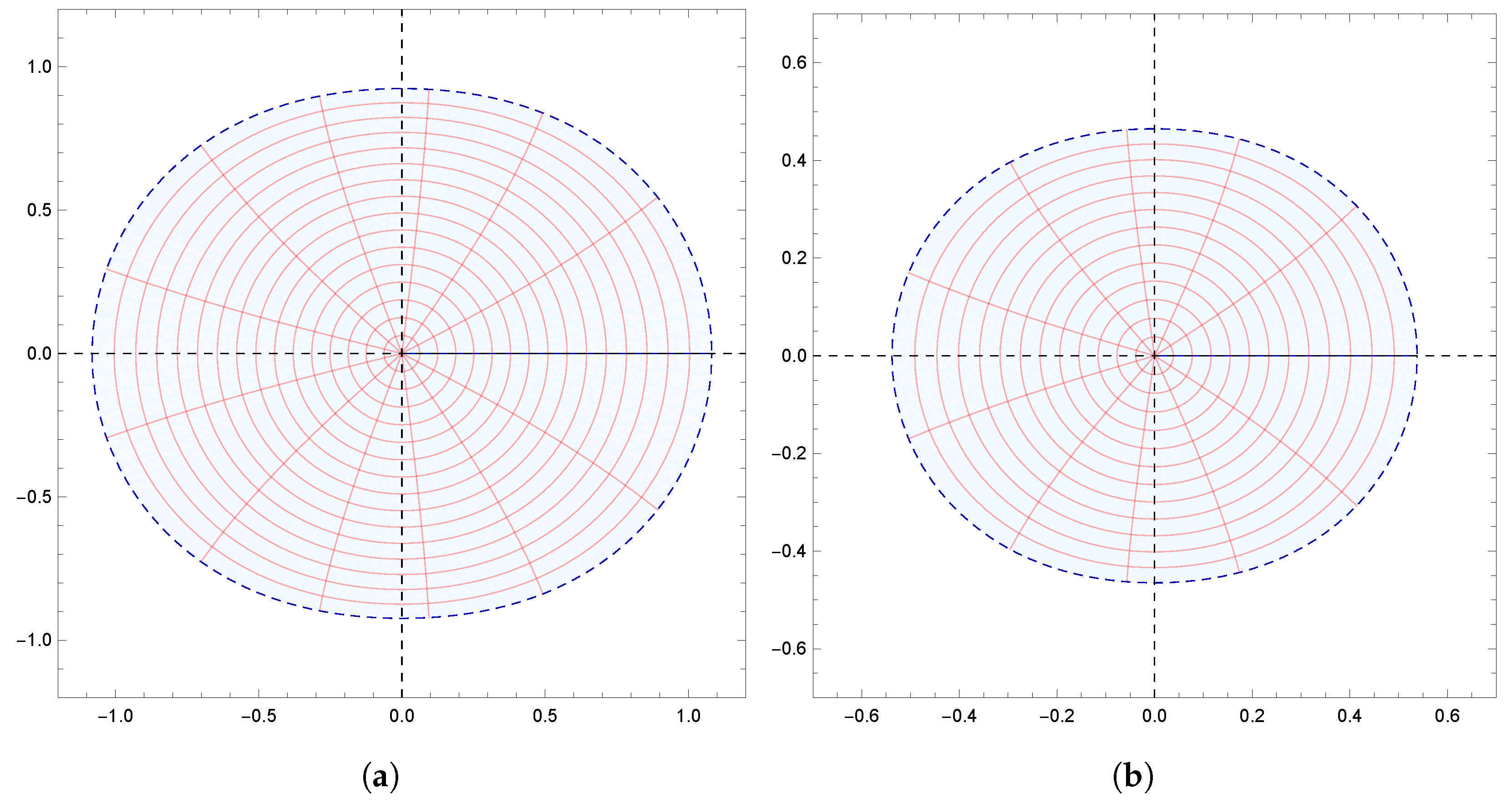
Moreover, the results obtained were also supported by graphical representations generated using Mathematica 12.0. These images effectively depicted the fulfillment of conditions derived from the results, demonstrating the corresponding geometric properties of ${\mathcal{T}}_{\nu }$. Specifically, Figure 1a,b demonstrate the starlikeness of ${\mathcal{T}}_{\nu }$ on $\mathbb{D}$ and ${\mathbb{D}}_{\frac{1}{2}}$, respectively. Figure 2 showcases the k-starlikeness of ${\mathcal{T}}_{\nu }$ on $\mathbb{D}$. 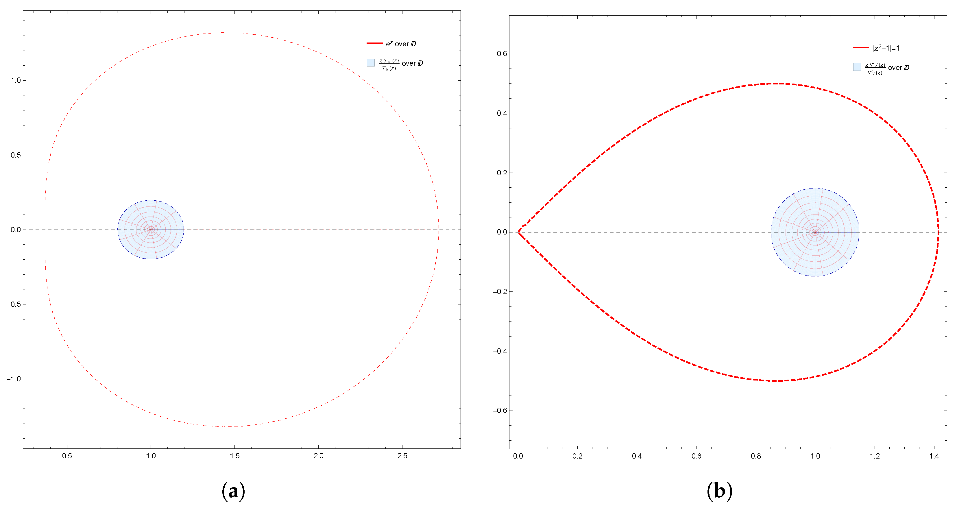Moreover, Figure 3a,b exhibit the starlikeness of ${\mathcal{T}}_{\nu }$ associated with the exponential function and the Bernoulli lemniscate on $\mathbb{D}$, respectively. The pre-starlikeness of ${\mathcal{T}}_{\nu }$ can be observed in Figure 4. Furthermore, Figure 5a,b illustrate the convexity of ${\mathcal{T}}_{\nu }$ on $\mathbb{D}$ and ${\mathbb{D}}_{\frac{1}{2}}$, respectively. Figure 6 presents the k-uniform convexity of ${\mathcal{T}}_{\nu }$ on $\mathbb{D}$. Additionally, Figure 7a,b display the convexity of ${\mathcal{T}}_{\nu }$ associated with the exponential function and the Bernoulli lemniscate on $\mathbb{D}$, respectively. These graphical representations provided a comprehensive visualization of the studied properties.