Homogenization of a Thermoelastic Bristly Structure Immersed in a Thermofluid

Abstract

The article considers the mathematical model describing the joint motion of a viscous compressible heat-conducting fluid and a thermoelastic plate with a fine two-level thermoelastic bristly microstructure attached to it. The bristly microstructure consists of a great amount of taller and shorter bristles, which are periodically located on the surface of the plate, and the model under consideration incorporates a small parameter, which is the ratio of the characteristic lengths of the microstructure and the entire plate. Using classical methods in the theory of partial differential equations, we prove that the initial-boundary value problem for the considered model is well-posed. After this, we fulfill the homogenization procedure, i.e., we pass to the limit as the small parameter tends to zero, and, as a result, we derive the effective macroscopic model in which the dynamics of the interaction of the ‘liquid–bristly structure’ is described by equations of two homogeneous thermoviscoelastic layers with memory effects. The homogenization procedure is rigorously justified by means of the Allaire–Briane three-scale convergence method. The developed effective macroscopic model can potentially find application in further mathematical modeling in biotechnology and bionics taking account of heat transfer.

1. Introduction

In this article, by a bristly structure on the surface of a flat plate, we mean a set consisting of a large number of frequently arranged bristles (hairs, needles, pins) orthogonally attached to the plate and forming a single whole with it—a bristly plate. A natural approach to mathematical description of interactions of such a plate with a liquid or gas flow around it consists in applying the theoretical provisions of continuum mechanics. In turn, the presence of a large number of bristles on the plate causes a special difficulty, which is as follows. If each individual bristle is taken into account in description, i.e., mathematical modeling is performed on a microscopic scale, then the resulting model may be mathematically correct, but unsuitable for practical analysis; from the computational point of view, the great amount of bristles leads to the necessity of using very fine meshes in numerical analysis, which leads to an inaccessible amount of calculations. This circumstance motivates the construction of macroscopic models in which each individual bristle is not distinguished, but an ‘average’ effective description of the flow around the bristle plate is given.

The mathematical modeling on macroscopic scales of bristly structures immersed in liquid or gas has a fairly notable history. Almost ninety years ago, in 1938, a rather simple model was proposed in the monograph by S. Goldstein (Sections 53 and 145, [1]). In this model, a laminar flow around a flat plate with a single orthogonally welded pin is considered. The air flows in parallel to the plate. The conditions are found for the airflow to remain laminar after passing by the pin. The obvious idea that the flow remains laminar again after flowing around another similar pin leads to the conclusion that Goldstein’s model can be naturally generalized to cases of any number of pins, that is, to cases of bristly structures. Such a generalization was successfully adapted in a number of works for studying aerodynamics in a neighborhood of a plant leaf with trichomes being taken into account; see, for example, [2] and Chapter X in [3]. Trichomes are bristles (fuzz) on a leaf epithelium. It is worth noting that Goldstein’s model [1] has its origins in the theory of the wing in aeronautics. As a matter of fact, Goldstein’s model and its generalizations [2,3] are strictly restrained to the laminar regimes and are inapplicable for studying more complex situations of flow. A much more general macroscopic model, covering a wide range of interactions between a bristly plate and a fluid flow around it, was constructed by K.H. Hoffmann, N.D. Botkin and V.N. Starovoitov in 2005 in [4] by the homogenization method starting from the classical Stokes equations of viscous compressible fluid and classical Lamé’s equations of linear elasticity. This model is isothermal, and it is based on a microstructure with frequently and periodically arranged cylindrical elastic bristles of the same size. In [4], the authors give the full justification of the homogenization procedure and fulfill a series of numerical experiments that show good consistency with physical observations.

The study in [4] was motivated by demand in mathematical modeling and design of aptamer-based biosensors; in the introduction in [4], the authors suggested that ‘one can impress’ (inside the biosensor) ‘the aptamer protein layer as a periodic bristle or pin structure on the top of the gold film contacting the liquid’. Since 2005, based on the Hoffmann–Botkin–Starovoitov model (from [4]), several computational algorithms for modeling biosensors have been created and the corresponding numerical experiments have been carried out [5,6,7]. More specifically, Ref. [5] describes a numerical method and a program for calculating dispersion relations for surface and bulk acoustic waves in multi-layered anisotropic structures that may contain specific bristle-like layers in contact with liquids. This study is of great importance from the point of view of biosensor applications, since the numerical method takes into account the piezoelectric properties of materials, the ability to work with very thin layers and adequate treatment of the interface between a solid bristle-like structure and a liquid. In [6], an interesting approach for simulation of wave patterns in surface acoustic wave biosensors is proposed. This approach relies on [4] and involves a rather subtle application of the differential games theory. The feasibility of this approach is verified in [6] by a set of numerical experiments. The most recent article [7] develops the concepts obtained in [4,5] for investigating the glycocalyx, ‘a polysaccharide polymer molecule layer on the endothelium of blood vessels that, according to recent studies, plays an important role in protecting against diseases (citation from [7]).

At the same time, since the Hoffmann–Botkin–Starovoitov model is based on the most fundamental laws of continuum mechanics and does not contain in its general form any specific dependencies related to certain properties of biosensor components, its applicability can be expanded for a much larger number of phenomena related to bristly structures, rather than only with processes in biosensors. In particular, the Hoffmann–Botkin–Starovoitov model can be regarded as a generalization of Goldstein’s model [1,2,3] for (not necessarily laminar) airflow near a plant’s leaves, in a sense.

Now, let us note that, for many reasons arising from nature and technological demands, it is favorable to consider bristly structures, including bristles having two distinct sizes. For example, in the general case, trichomes on the same leaf of a plant may belong to different types depending on length and form, which should be taken into account when studying airflow near the leaf. A characteristic feature is that the number of trichomes of different lengths has a different order; on a plant leaf, there are quite a lot of short trichomes for one long trichome [8,9,10]. Another possible application of models of two-level bristly structures interacting with liquids can be found in bionics (or biomimicry). Biomimicry describes the processes in which ideas and concepts developed by nature are translated into technology. According to the observations made in [11], bristles, as a rule, have a strong effect on the wettability of plates; plate surfaces can be superhydrophobic, self-cleaning (superoleophobic) and have low adhesion, which are often very advantageous properties for materials. Two-level (hierarchical) roughness structures are typical for superhydrophobic surfaces in nature. For example, the effect of self-purification in polluted reservoirs using a two-level trichome structure is observed in lotus. In Section 42.4.3 in [12], the question of how to create an artificial two-level superhydrophobic surface similar to the surface of a lotus is discussed in detail.

Inspired by the observations and ideas from [8,9,10,11,12], in 2020 in [13], we generalized the Hoffmann–Botkin–Starovoitov model from [4] to the case of isothermal two-level bristly structures. The model that we further construct in the present article is a natural generalization to non-isothermal cases of the Hoffmann–Botkin–Starovoitov isothermal models built earlier for single-level [4] and two-level [13] bristly structures. We call this new model Model H. It is formulated in detail in Section 5 and is the main result of this article. Its obvious advantage over the above-mentioned previously built models lies in taking into account heat transfer; all the above-mentioned models are isothermal. The limitation of Model H lies in its linearity. By their nature, linear models are quite suitable for describing slow hydrodynamic flows and small elastic and thermoelastic deformations. Thus, rapid flows, including high turbulence, and large deformations are practically not covered by Model H. Note that the above-mentioned models from [1,2,3,4,13] are also linear.

The contents of our study are as follows. In Section 2, we introduce and thoroughly describe the geometry of a bristly microstructure. To derive Model H from the microstructure, in the present article, similarly to [4,13], we use the homogenization method. Namely, a small parameter in the basic model (called Model $A_{\epsilon }$ in Section 3) is the ratio of the characteristic lengths of the bristly microstructure and the entire bristly plate. Using the Allaire–Briane three-scale convergence method [14], in Section 4, we carry out the limiting passage as the small parameter tends to zero, and as a result, we construct the homogenized three-scale model. In this three-scale model, it is no longer necessary to consider the thermomechanical evolution of each individual bristle; it provides an approximate average description of the ‘smoothed’ thermomechanical system and, in principle, is suitable for numerical analysis. At the same time, the three-scale model is nonclassical and looks very unusual. In order to clarify its physical essence and make possible applications easier, in Section 5, we fulfill the full asymptotic decomposition, which amounts to the gradual scale separation. The desired Model H arises as the result of this procedure. Section 6 is devoted to concluding remarks and discussion. Appendix A contains some auxiliary technical provisions.

2. The Flow Domain: Fine Geometry of the Bristly Microstructure

Assume that the entire thermomechanical continuum, consisting of a heat-conducting viscous fluid and a thermoelastic bristly plate, occupies the unit cube $\Omega ={(0,1)}^3$ in the space ${\mathbb{R}}^3$ of dimensionless physical positions $x=(x_1,x_2,x_3)$. Cube $\Omega$ is divided into two disjoint subdomains ${\Omega }_F^{\epsilon }$ and ${\Omega }_S^{\epsilon }$ and the boundary ${\Gamma }_{\epsilon }$ between them, so that the fluid occupies subdomain ${\Omega }_F^{\epsilon }$ and the plate with attached bristles occupies subdomain ${\Omega }_S^{\epsilon }$.

Let us precisely define the geometrical forms of ${\Omega }_S^{\epsilon }$ and ${\Omega }_F^{\epsilon }$, following the lines of Section 3 in [13]. By this, we will simultaneously introduce a two-level bristly microstructure.

Assume that the flat plate lies at the bottom of cube $\Omega$ and fills in layer

$${\Omega }_{\mathrm{pl}}=\{x\in \Omega :0<x_3<\Delta \}(\Delta =\mathrm{const}<1).$$

The bristles are modeled as cylinders that are very frequently periodically located on the upper surface $\{x\in \Omega :x_3=\Delta \}$ of the flat plate ${\Omega }_{\mathrm{pl}}$, orthogonally to this surface. There are cylinders of two different sizes. The shorter and at the same time thinner cylinders are located on the upper surface of the flat plate, an order or several orders of magnitude more often than the taller and thicker ones. The heights of the cylinders are fixed and equal to ${\delta }_{*}$ and ${\delta }^{*}$, where $\Delta +{\delta }_{*}<\Delta +{\delta }^{*}<1$. The formal description of the shapes of the cylinders and their location is as follows.

Taller bristles are located $\epsilon$-periodically and shorter bristles are located ${\epsilon }^2$-periodically in $x_1$ and $x_2$. Thus, parameter $\epsilon$ characterizes the distance between two adjacent taller bristles (cylinders) and value ${\epsilon }^2$ characterizes the distance between two adjacent shorter bristles. Parameter $\epsilon$ is small and positive: $\epsilon >0$, $\epsilon \ll 1$. In order to describe exact locations of the bristles, we introduce mesoscopic variables $\widehat{\mathit{y}}=(y_1,y_2)\in {\mathbb{R}}^2$, microscopic variables $\widehat{\mathit{z}}=(z_1,z_2)\in {\mathbb{R}}^2$, and, correspondingly, the pattern mesoscopic cell $\Sigma =(0,1)\times (0,1)\subset {\mathbb{R}}_{\widehat{y}}^2$ and the pattern microscopic cell $\Theta =(0,1)\times (0,1)\subset {\mathbb{R}}_{\widehat{z}}^2$, each consisting of the two nonempty subdomains and the interface between these subdomains:

$$\Sigma ={\Sigma }_F\cup {\Sigma }_S\cup {\Gamma }_{\Sigma },\Theta ={\Theta }_F\cup {\Theta }_S\cup {\Gamma }_{\Theta }.$$

Here, ${\Sigma }_S$ is the orthogonal projection of a taller bristle onto the upper surface of the flat plate ${\Omega }_{\mathrm{pl}}$ taken in ${\epsilon }^{-1}:1$ scale, i.e., ${\epsilon }^{-1}$ -times stretched. Analogously, ${\Theta }_S$ is the orthogonal projection of a shorter bristle onto the upper surface of the flat plate ${\Omega }_{\mathrm{pl}}$ taken in ${\epsilon }^{-2}$:1 scale. We assume that both ${\Sigma }_S$ and ${\Theta }_S$ are simply connected sets with smooth boundaries, each of them being locally situated on one side of the boundary. For simplicity, suppose that ${\Sigma }_S$ and ${\Theta }_S$ do not have common points with $\partial \Sigma$ and $\partial \Theta$, respectively (see Figure 1 and Figure 2).

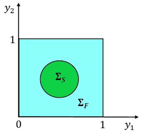
Figure 1. Mesoscopic pattern cell.

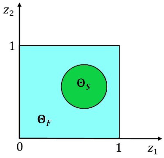
Figure 2. Microscopic pattern cell.

Further, let us additionally denote $\widehat{\mathit{x}}=(x_1,x_2)$ and introduce into consideration the characteristic functions $\widehat{\zeta }=\widehat{\zeta }(\widehat{\mathit{y}})$ and $\widehat{\psi }=\widehat{\psi }(\widehat{\mathit{z}})$ of sets ${\Sigma }_F$ and ${\Theta }_F$, respectively:

$$\widehat{\zeta }(\widehat{\mathit{y}})=\left\{\begin{array}{c}1\mathrm{for} \widehat{\mathit{y}}\in {\Sigma }_F,\hfill \\ 0\mathrm{for} \widehat{\mathit{y}}\in \overline{\Sigma }\setminus {\Sigma }_F,\hfill \end{array}\right.\widehat{\psi }(\widehat{\mathit{z}})=\left\{\begin{array}{c}1\mathrm{for} \widehat{\mathit{z}}\in {\Theta }_F,\hfill \\ 0\mathrm{for} \widehat{\mathit{z}}\in \overline{\Theta }\setminus {\Theta }_F.\hfill \end{array}\right.$$

(1)

Extend functions $\widehat{\zeta }$ and $\widehat{\psi }$ onto the whole spaces ${\mathbb{R}}_{\widehat{y}}^2$ and ${\mathbb{R}}_{\widehat{z}}^2$ 1-periodically.

Using the above introduced constructions, we define the characteristic function

$${\chi }^{\epsilon }(\mathit{x})=\left\{\begin{array}{c}1\mathrm{for} \mathit{x}\in {\Omega }_F^{\epsilon },\hfill \\ 0\mathrm{for} \mathit{x}\in \overline{\Omega }\setminus {\Omega }_F^{\epsilon }\hfill \end{array}\right.$$

(2)

of domain ${\Omega }_F^{\epsilon }$ as follows:

$${\chi }^{\epsilon }(\mathit{x})=\zeta \left({\displaystyle \frac{\widehat{x}}{\epsilon }},x_3\right)\psi \left({\displaystyle \frac{\widehat{\mathit{x}}}{{\epsilon }^2}},x_3\right),$$

(3a)

where

$$\begin{array}{cc}\hfill & \zeta \left({\displaystyle \frac{\widehat{\mathit{x}}}{\epsilon }},x_3\right)=\left\{\begin{array}{ccc}1& \mathrm{for}& {\delta }^{*}+\Delta <x_3<1,\hfill \\ {\displaystyle \widehat{\zeta }\left(\frac{\widehat{\mathit{x}}}{\epsilon }\right)}& \mathrm{for}& \Delta \le x_3\le {\delta }^{*}+\Delta ,\hfill \\ 0& \mathrm{for}& 0<x_3<\Delta ,\hfill \end{array}\right.\hfill \end{array}$$

(3b)

$$\begin{array}{cc}\hfill & \psi \left({\displaystyle \frac{\widehat{\mathit{x}}}{{\epsilon }^2}},x_3\right)=\left\{\begin{array}{ccc}1& \mathrm{for}& {\delta }_{*}+\Delta <x_3<1,\hfill \\ {\displaystyle \widehat{\psi }\left(\frac{\widehat{\mathit{x}}}{{\epsilon }^2}\right)}& \mathrm{for}& \Delta \le x_3\le {\delta }_{*}+\Delta ,\hfill \\ 0& \mathrm{for}& 0<x_3<\Delta .\hfill \end{array}\right.\hfill \end{array}$$

(3c)

Correspondingly, ${\Omega }_S^{\epsilon }=\Omega \setminus \overline{{\Omega }_F^{\epsilon }}$. Thus, the structure of ${\Omega }_S^{\epsilon }$ and ${\Omega }_F^{\epsilon }$ is introduced. It is loosely shown in Figure 3.

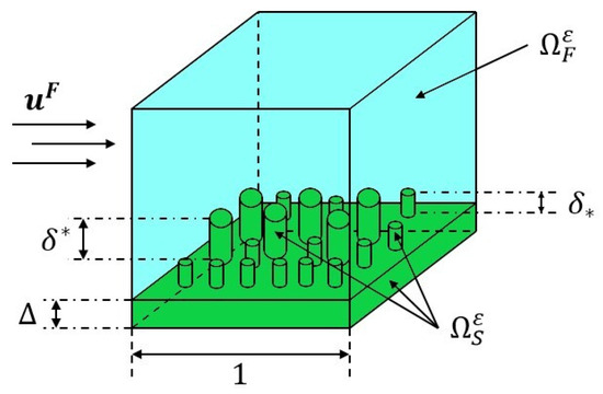
Figure 3. The bristly plate (painted green) and the fluid flow.

3. Basic Formulation of the ‘Thermofluid–Thermoelastic Structure’ Interactions

The starting point of our research is the following linearized model of joint motion of a heat-conducting viscous compressible fluid and a thermoelastic bristly plate.

Model ${\mathrm{A}}_{\mathbf{\epsilon }}$.

(Basic formulation of the ‘thermofluid–thermoelastic structure’ interactions. The dimensionless form).

Assume that the geometry of the spatial domain $\Omega \subset {\mathbb{R}}_x^3$, its subdomains ${\Omega }_F^{\epsilon }$ and ${\Omega }_S^{\epsilon }$, and the interface ${\Gamma }_{\epsilon }$ between ${\Omega }_F^{\epsilon }$ and ${\Omega }_S^{\epsilon }$ is defined as in Section 2. Denote the independent time variable by t. Let $T=const>0$ be an arbitrarily given moment of time.

■

The sought functions in the heat-conducting fluid (thermofluid) are the velocity field ${\mathit{u}}_{\epsilon }$: ${\Omega }_F^{\epsilon }\times (0,T)\mapsto {\mathbb{R}}^3$ and the temperature distribution ${\theta }_{\epsilon }$: ${\Omega }_F^{\epsilon }\times (0,T)\mapsto \mathbb{R}$. The thermofluid motion in ${\Omega }_F^{\epsilon }$ for $t\in (0,T)$ is governed by the system of the Stokes–Fourier equations, which consists of the balance of momentum equation

$${\alpha }_{\tau }{\rho }_F{\partial }_t{\mathit{u}}_{\epsilon }={\mathrm{div}}_x\left(2{\alpha }_{\mu }{\mathbb{D}}_x({\mathit{u}}_{\epsilon })+({\alpha }_{\lambda }{\mathrm{div}}_x{\mathit{u}}_{\epsilon }+{\alpha }_p{\mathrm{div}}_x{J}_t{\mathit{u}}_{\epsilon }-p^0)\mathbb{I}-{\mathbb{B}}_F{\theta }_{\epsilon }\right)+{\alpha }_g{\rho }_F\mathit{f}$$

(4a)

and the energy equation

$$c_F{\partial }_t{\theta }_{\epsilon }={\mathrm{div}}_x({\varkappa }_F{\nabla }_x{\theta }_{\epsilon })-{\mathbb{B}}_F:{\mathbb{D}}_x({\mathit{u}}_{\epsilon })+{\mathbf{\Psi }}_F.$$

(4b)

■

The sought functions in the thermoelastic bristly plate are the displacement field ${\mathit{v}}_{\epsilon }$: ${\Omega }_S^{\epsilon }\times (0,T)\mapsto {\mathbb{R}}^3$ and the temperature distribution ${\theta }_{\epsilon }$: ${\Omega }_S^{\epsilon }\times (0,T)\mapsto \mathbb{R}$. The motion of the bristly plate particles in ${\Omega }_S^{\epsilon }$ for $t\in (0,T)$ is governed by the system of classical equations of linear thermoelasticity, which consists of the balance of momentum equation

$${\alpha }_{\tau }{\rho }_S{\partial }_t^2{\mathit{v}}_{\epsilon }={\mathrm{div}}_x\left(\mathcal{G}:{\nabla }_x{\mathit{v}}_{\epsilon }-{\mathbb{B}}_S{\theta }_{\epsilon }\right)+{\alpha }_g{\rho }_S\mathit{f}$$

(4c)

and the energy equation

$$c_S{\partial }_t{\theta }_{\epsilon }={\mathrm{div}}_x({\varkappa }_S{\nabla }_x{\theta }_{\epsilon })-{\mathbb{B}}_S:{\partial }_t{\mathbb{D}}_x({\mathit{v}}_{\epsilon })+{\mathbf{\Psi }}_S.$$

(4d)

■

On interface ${\Gamma }_{\epsilon }$ for $t\in (0,T)$, the continuity conditions for the velocity and temperature

$${\mathit{u}}_{\epsilon }={\partial }_t{\mathit{v}}_{\epsilon },{\theta }_{\epsilon }^{(f)}={\theta }_{\epsilon }^{(s)},$$

(4e)

for the normal stress

$${\left(2{\alpha }_{\mu }{\mathbb{D}}_x({\mathit{u}}_{\epsilon })+({\alpha }_{\lambda }{\mathrm{div}}_x{\mathit{u}}_{\epsilon }+{\alpha }_p{\mathrm{div}}_x{J}_t{\mathit{u}}_{\epsilon }-p^0)\mathbb{I}-{\mathbb{B}}_F{\theta }_{\epsilon }^{(f)}\right)}_{{\mathit{n}}_{\epsilon }}={\left(\mathcal{G}:{\nabla }_x{\mathit{v}}_{\epsilon }-{\mathbb{B}}_S{\theta }_{\epsilon }^{(s)}\right)}_{{\mathit{n}}_{\epsilon }},$$

(4f)

and for the normal heat flux

$${\varkappa }_F{\nabla }_x{\theta }_{\epsilon }^{(f)}{·}_{{\mathit{n}}_{\epsilon }}={\varkappa }_S{\nabla }_x{\theta }_{\epsilon }^{(s)}{·}_{{\mathit{n}}_{\epsilon }}$$

(4g)

are imposed.

■

The system of Equations (4a)–(4d) and interfacial conditions (4e)–(4g) is supplemented by the initial conditions

$$\begin{array}{cc}\hfill & {\mathit{u}}_{\epsilon }{|}_{t=0}={\mathit{u}}^0(\mathit{x}),\mathit{x}\in {\Omega }_F^{\epsilon },\hfill \end{array}$$

(4h)

$$\begin{array}{cc}\hfill & {\mathit{v}}_{\epsilon }{|}_{t=0}={\mathit{v}}^0(\mathit{x}),{\partial }_t{\mathit{v}}_{\epsilon }{|}_{t=0}={\mathit{w}}^0(\mathit{x}),x\in {\Omega }_S^{\epsilon },\hfill \end{array}$$

(4i)

$$\begin{array}{cc}\hfill & {\theta }_{\epsilon }{|}_{t=0}={\theta }^0(x),\mathit{x}\in \Omega ,\hfill \end{array}$$

(4j)

and the conditions on the fixed boundary $\partial \Omega$:

$$\begin{array}{cc}\hfill & {\mathit{u}}_{\epsilon }(\mathit{x},t)={\mathit{u}}^F(\mathit{x},t),\mathit{x}\in \partial \Omega \cap \partial {\Omega }_F^{\epsilon },t\in (0,T),\hfill \end{array}$$

(4k)

$$\begin{array}{cc}\hfill & {\mathit{v}}_{\epsilon }(\mathit{x},t)=0,\mathit{x}\in \partial \Omega \cap \partial {\Omega }_S^{\epsilon },t\in (0,T),\hfill \end{array}$$

(4l)

$$\begin{array}{cc}\hfill & {\theta }_{\epsilon }(\mathit{x},t)={\theta }^{\star }(\mathit{x},t),\mathit{x}\in \partial \Omega ,t\in (0,T).\hfill \end{array}$$

(4m)

Remark 1.

System (4) arises from the fundamentals of continuum mechanics by virtue of natural clarifying and simplifying assumptions and the classical formalism of linearization. The details of the derivation of system (4) can be found in Sections 2 and 3 in [15].

In (4a) and further in the paper, by ${\mathbb{D}}_x(\mathit{\varphi })$, we denote the symmetric part of the gradient of some adequate regular vector-function $\mathit{\varphi }(x)$: $D_{xij}(\mathit{\varphi })=(1/2)({\partial }_{x_i}{\varphi }_j+{\partial }_{x_j}{\varphi }_i)$, $i,j=1,2,3$. The rest of the notation for differential operators in (4) is quite standard. In (4a) and further in the paper, by $J_t$, we denote the Volterra operator:

$$(J_t\varphi )(t)={\int }_0^t\varphi (s)ds,\forall \varphi \in L^1(0,T).$$

(5)

By $\mathbb{I}$, we denote the identical transformation in ${\mathbb{R}}^3$, i.e., $\mathbb{I}=({\delta }_{ij})$, where ${\delta }_{ij}$ is Kronecker’s symbol. In (4e)–(4g), the following notation for values of temperature ${\theta }_{\epsilon }$ on interface ${\Gamma }_{\epsilon }$ is used; for any ${\mathit{x}}_0\in {\Gamma }_{\epsilon }$, we set

$${\theta }_{\epsilon }^{(f)}({\mathit{x}}_0)=\underset{\begin{array}{c}\mathit{x}\to {\mathit{x}}_0\hfill \\ \mathit{x}\in {\Omega }_F^{\epsilon }\hfill \end{array}}{lim}{\theta }_{\epsilon }(\mathit{x}),{\theta }_{\epsilon }^{(s)}({\mathit{x}}_0)=\underset{\begin{array}{c}\mathit{x}\to {\mathit{x}}_0\hfill \\ \mathit{x}\in {\Omega }_S^{\epsilon }\hfill \end{array}}{lim}{\theta }_{\epsilon }(\mathit{x}).$$

Vector ${\mathit{n}}_{\epsilon }({\mathit{x}}_0)$ is the unit normal to ${\Gamma }_{\epsilon }$ at a point ${\mathit{x}}_0$, pointing into ${\Omega }_F^{\epsilon }$.

Dimensionless coefficients ${\alpha }_{\tau }$, ${\alpha }_{\mu }$, ${\alpha }_{\lambda }$, ${\alpha }_p$, ${\alpha }_g$, ${\varkappa }_F$, ${\varkappa }_S$, ${\rho }_F$, ${\rho }_S$, $c_F$, and $c_S$ are constant, positive and independent of $\epsilon$. They are given and relate to the dimensional physical characteristics of the problem via the following identities:

$$\begin{array}{cc}\hfill & {\alpha }_{\tau }={\displaystyle \frac{{\rho }_{sc}{L}_{sc}^2}{{\tau }_{sc}^2{p}_{sc}}},{\alpha }_{\mu }={\displaystyle \frac{\mu }{{\tau }_{sc}{p}_{sc}}},{\alpha }_{\lambda }={\displaystyle \frac{\lambda }{{\tau }_{sc}{p}_{sc}}},{\alpha }_p={\displaystyle \frac{1}{\gamma p_{sc}}},{\alpha }_g={\displaystyle \frac{{\rho }_{sc}g{L}_{sc}}{p_{sc}}},\hfill \\ \hfill & {\varkappa }_F={\displaystyle \frac{{\tau }_{sc}{\vartheta }_{sc}^2}{L_{sc}^2{T}_{*}{p}_{sc}}}{\varkappa }_F^{\prime },{\varkappa }_S={\displaystyle \frac{{\tau }_{sc}{\vartheta }_{sc}^2}{L_{sc}^2{T}_{*}{p}_{sc}}}{\varkappa }_S^{\prime },{\rho }_F={\displaystyle \frac{{\rho }_F^{\prime }}{{\rho }_{sc}}},{\rho }_S={\displaystyle \frac{{\rho }_S^{\prime }}{{\rho }_{sc}}},\hfill \\ \hfill & c_F={\displaystyle \frac{{\vartheta }_{sc}^2}{T_{*}{p}_{sc}}}{c}_F^{\prime },c_S={\displaystyle \frac{{\vartheta }_{sc}^2}{T_{*}{p}_{sc}}}{c}_S^{\prime }.\hfill \end{array}$$

Here, $L_{sc}$ is the characteristic size of $\Omega$ (measured, for example, in meters: m); ${\tau }_{sc}$ (s) is the characteristic duration of physical processes; $p_{sc}$ (kg· ${\mathrm{m}}^{-1}·$ ${\mathrm{s}}^{-2}$) is the atmosphere pressure; g (m· ${\mathrm{s}}^{-2}$) is the acceleration of free fall; ${\rho }_{sc}$ (kg · ${\mathrm{m}}^{-3}$) is the mean density of air at the temperature 273 K and at the atmosphere pressure; $T_{*}$ (K) is a reference temperature; ${\vartheta }_{sc}$ (K) is the temperature difference between the boiling and freezing points of water at atmospheric pressure. Dimensional coefficients $\mu$, $\lambda$, ${\rho }_F^{\prime }$, ${\varkappa }_F^{\prime }$, and $c_F^{\prime }$ in the fluid phase are respective shear and bulk viscosities, mean density, heat conductivity, and specific heat capacity at constant pressure; the dimensional coefficient $\gamma$ characterizes the compressibility of the fluid. Dimensional coefficients ${\rho }_S^{\prime }$, ${\varkappa }_S^{\prime }$, and $c_S^{\prime }$ in the solid phase are respective mean density, heat conductivity and specific heat capacity at constant pressure.

Tensor $\mathcal{G}=({\mathcal{G}}^{ijkl})$ is the dimensionless elastic stiffness tensor. Its components ${\mathcal{G}}^{ijkl}$ ($i,j,k,l=1,2,3$) can be arbitrary up to base restrictions so that any anisotropic solid can be considered. We have

$${(\mathcal{G}:{\nabla }_{x}v)}_{ij}=\sum _{k,l=1}^3{\mathcal{G}}^{ijkl}{\partial }_{x_l}{v}_k,i,j=1,2,3,$$

components ${\mathcal{G}}^{ijkl}$ are constant, and we fulfill the symmetry condition

$${\mathcal{G}}^{ijkl}={\mathcal{G}}^{ijlk}={\mathcal{G}}^{klij}={\mathcal{G}}^{jikl},i,j,k,l=1,2,3,$$

(6)

and the positive-definiteness condition; there exists a constant $c_{\mathcal{G}}>0$ such that

$${\displaystyle (\mathcal{G}:\mathbb{X}):\mathbb{X}\equiv \sum _{i,j,k,l=1}^3{\mathcal{G}}^{ijkl}{X}_{kl}{X}_{ij}\ge c_{\mathcal{G}}{\left|\mathbb{X}\right|}^2,\forall \mathbb{X}\in {\mathbb{R}}_{\mathrm{symm}}^{3\times 3}.}$$

(7)

Here and further, we deal with symmetric $3\times 3$ matrices, say, $\mathbb{X}={(X_{ij})}_{i,j=1,2,3}$ such that $X_{ij}=X_{ji}$. We denote the class of these matrices by ${\mathbb{R}}_{\mathrm{symm}}^{3\times 3}$. Note that demands (5) and (7) perfectly meet the fundamental principles of Newtonian mechanics.

Notation 1.

Above in this section and further in the article, we use the conventional notation for the inner products of fourth-rank tensors and $3\times 3$ matrices. More precisely, $\mathcal{A}:\mathbb{W}$ is the inner product (convolution) of a fourth-rank tensor $\mathcal{A}$ and a $3\times 3$ matrix $\mathbb{W}$. It is the $3\times 3$ matrix defined by the formula

$$\mathcal{A}:\mathbb{W}={\left(\sum _{k,l=1,2,3}{\mathcal{A}}^{ijkl}{W}_{kl}\right)}_{i,j=1,2,3}.$$

The inner product (convolution) of two $3\times 3$ matrices $\mathbb{W}$ and $\mathbb{C}$ is the scalar defined by formula

$$\mathbb{W}:\mathbb{C}=\sum _{i,j=1}^3{W}_{ij}{C}_{ij}.$$

In particular, we have

$$(\mathcal{A}:\mathbb{W}):\mathbb{C}=\sum _{i,j,k,l=1}^3{\mathcal{A}}^{ijkl}{W}_{kl}{C}_{ij},{\left|\mathbb{W}\right|}^2=\mathbb{W}:\mathbb{W}=\sum _{i,j=1}^3{W}_{ij}{W}_{ij},\mathrm{tr}\mathbb{W}=\mathbb{W}:\mathbb{I}$$

for all fourth-rank tensors $\mathcal{A}$ and $3\times 3$ matrices $\mathbb{W}$ and $\mathbb{C}$.

In the formulation of Problem ${\mathrm{A}}_{\epsilon }$, the dimensionless elastic stiffness tensor $\mathcal{G}$ relates to the dimensional elastic stiffness tensor ${\mathcal{G}}^{\prime }$ via the identity $\mathcal{G}={\mathcal{G}}^{\prime }/p_{sc}$, $3\times 3$ matrices ${\mathbb{B}}_F=(B_F^{ij})$ and ${\mathbb{B}}_S=(B_S^{ij})$ are the dimensionless matrices characterizing thermal dilatation in the fluid and solid phases, respectively; these matrices are constant, symmetric, and they relate to the dimensional matrices ${\mathbb{B}}_F^{\prime }$ and ${\mathbb{B}}_S^{\prime }$ via identities

$${\mathbb{B}}_F={\displaystyle \frac{{\vartheta }_{sc}}{p_{sc}}}{\mathbb{B}}_F^{\prime },{\mathbb{B}}_S={\displaystyle \frac{{\vartheta }_{sc}}{p_{sc}}}{\mathbb{B}}_S^{\prime }.$$

The sought dimensionless velocity ${\mathit{u}}_{\epsilon }$, displacement ${\mathit{v}}_{\epsilon }$ and temperature ${\theta }_{\epsilon }$ relate to the respective dimensional distributions ${\mathit{u}}_{\epsilon }^{\prime }$, ${\mathit{v}}_{\epsilon }^{\prime }$ and ${\theta }_{\epsilon }^{\prime }$ via identities

$${\mathit{u}}_{\epsilon }={\displaystyle \frac{{\tau }_{sc}}{L_{sc}}}{\mathit{u}}_{\epsilon }^{\prime },{\mathit{v}}_{\epsilon }={\displaystyle \frac{1}{L_{sc}}}{\mathit{v}}_{\epsilon }^{\prime },{\theta }_{\epsilon }={\displaystyle \frac{{\theta }_{\epsilon }^{\prime }-T_{*}}{{\vartheta }_{sc}}}.$$

Vector-function f is the dimensionless density of distributed mass forces and scalar functions ${\mathbf{\Psi }}_F$ and ${\mathbf{\Psi }}_S$ are volumetric dimensionless densities of external heat application in the fluid and the solid phases, respectively. We have

$$\mathit{f}={\displaystyle \frac{{\mathit{f}}^{\prime }}{g}},{\mathbf{\Psi }}_F={\displaystyle \frac{{\tau }_{sc}{\vartheta }_{sc}}{T_{*}{p}_{sc}}}{\mathbf{\Psi }}_F^{\prime },{\mathbf{\Psi }}_S={\displaystyle \frac{{\tau }_{sc}{\vartheta }_{sc}}{T_{*}{p}_{sc}}}{\mathbf{\Psi }}_S^{\prime },$$

where ${\mathit{f}}^{\prime }$, ${\mathbf{\Psi }}_F^{\prime }$ and ${\mathbf{\Psi }}_S^{\prime }$ are the corresponding dimensional thermomechanical characteristics.

The initial distributions $p^0$, ${\mathit{u}}^0$, ${\mathit{v}}^0$, ${\mathit{w}}^0$, and ${\theta }^0$ in (4a), (4f) and (4h)–(4j) and the boundary distributions ${\mathit{u}}^F$ and ${\theta }^{\star }$ in (4k) and (4m) are given.

We accept the following two assumptions on the initial data in Model ${\mathsf{A}}_{\epsilon }$.

Assumption  1.

We suppose that the initial data for velocity

$${\displaystyle {\mathit{u}}^0(\mathit{x})=\left\{\begin{array}{ccc}\hfill {\mathit{u}}^0(\mathit{x})& \mathrm{for}& \mathit{x}\in {\Omega }_F^{\epsilon },\hfill \\ \hfill {\mathit{w}}^0(\mathit{x})& \mathrm{for}& \mathit{x}\in {\Omega }_S^{\epsilon },\hfill \end{array}\right.}$$

given in the whole cube Ω, does not depend on ε. In other words, we impose a uniform initial velocity field ${\mathit{u}}^0$ on Ω independent of ε.

Assumption 1 is consistent with the requirement that the initial velocity field is continuous in the whole cube $\Omega$.

Assumption 2.

We suppose that the initial distribution of pressure $p^0$ and the initial displacement ${\mathit{v}}^0$ are defined in the whole cube Ω, do not depend on ε, and along with ${\mathit{u}}^0$ and ${\theta }^0$, satisfy the compatibility conditions

$$\begin{array}{cc}\hfill & 2{\alpha }_{\mu }{\mathbb{D}}_x({\mathit{u}}^0)+({\alpha }_{\lambda }{\mathrm{div}}_x{\mathit{u}}^0-p^0)\mathbb{I}-{\mathbb{B}}_F{\theta }^0=\mathcal{G}:{\nabla }_x{v}^0-{\mathbb{B}}_S{\theta }^0\in H^1{(\Omega )}^{3\times 3},\hfill \end{array}$$

(8a)

$$\begin{array}{cc}\hfill & {\varkappa }_F{\nabla }_x{\theta }^0-{\mathbb{B}}_F{\mathit{u}}^0={\varkappa }_S{\nabla }_x{\theta }^0-{\mathbb{B}}_S{\mathit{u}}^0\in H^1{(\Omega )}^3.\hfill \end{array}$$

(8b)

Relations (8a) and (8b) express, respectively, the smoothness of the initial stress and the initial heat flux in the whole cube $\Omega$.

For the further purpose of homogenization, i.e., for the limiting transition as $\epsilon \searrow 0$, it is necessary to introduce the proper notion of weak solution to Model ${\mathrm{A}}_{\epsilon }$, uniform in the whole domain $\Omega$. To this end, let us follow Section 2.2 in [4] and $\S 2$ in [13].

Using (5), we rewrite Equation (4c) and condition (4i)₁ equivalently as

$${\alpha }_{\tau }{\rho }_S{\partial }_t{\mathit{u}}_{\epsilon }={\mathrm{div}}_x\left(\mathcal{G}:J_t{\nabla }_x{\mathit{u}}_{\epsilon }-{\mathbb{B}}_S{\theta }_{\epsilon }\right)+{\mathrm{div}}_x(\mathcal{G}:{\nabla }_x{v}^0)+{\alpha }_g{\rho }_S\mathit{f}$$

and Equation (4d) as

$$c_S{\partial }_t{\theta }_{\epsilon }={\mathrm{div}}_x({\varkappa }_S{\nabla }_x{\theta }_{\epsilon })-{\mathbb{B}}_S:{\mathbb{D}}_x({\mathit{u}}_{\epsilon })+{\mathbf{\Psi }}_S.$$

Here, ${\mathit{u}}_{\epsilon }={\partial }_t{v}_{\epsilon }$ is the velocity vector.

Using these equations and taking into account the notion of the characteristic function ${\chi }^{\epsilon }$ (recall Equations (2) and (3)), we rewrite system (4) as the system of the uniform momentum and energy equations with the discontinuous coefficients in the whole cube $\Omega$:

$$\begin{array}{cc}\hfill & {\alpha }_{\tau }{\rho }_{*}^{\epsilon }{\partial }_t{\mathit{u}}_{\epsilon }={\mathrm{div}}_x\left({\mathcal{M}}_{\epsilon }^t{\nabla }_x{\mathit{u}}_{\epsilon }+{\mathbb{M}}_{\epsilon }^0-{\mathbb{B}}_{*}^{\epsilon }{\theta }_{\epsilon }\right)+{\alpha }_g{\rho }_{*}^{\epsilon }\mathit{f},\mathit{x}\in \Omega ,t\in (0,T),\hfill \end{array}$$

(9a)

$$\begin{array}{cc}\hfill & c^{\epsilon }{\partial }_t{\theta }_{\epsilon }={\mathrm{div}}_x({\varkappa }^{\epsilon }{\nabla }_x{\theta }_{\epsilon })-{\mathbb{B}}_{*}^{\epsilon }:{\mathbb{D}}_x({\mathit{u}}_{\epsilon })+{\mathbf{\Psi }}^{\epsilon },\mathit{x}\in \Omega ,t\in (0,T),\hfill \end{array}$$

(9b)

supplemented with the set of initial and boundary data:

$$\begin{array}{cc}\hfill & {\mathit{u}}_{\epsilon }{|}_{t=0}={\mathit{u}}^0,{\theta }_{\epsilon }{|}_{t=0}={\theta }^0,\mathit{x}\in \Omega ,\hfill \end{array}$$

(9c)

$$\begin{array}{cc}\hfill & {\mathit{u}}_{\epsilon }(\mathit{x},t)={\mathit{u}}^{\star }(\mathit{x},t),{\theta }_{\epsilon }(\mathit{x},t)={\theta }^{\star }(\mathit{x},t),(\mathit{x},t)\in \partial \Omega \times (0,T).\hfill \end{array}$$

(9d)

In (9a) and (9b) and further, we denote

$$\begin{array}{cc}\hfill & {\rho }_{*}^{\epsilon }={\chi }^{\epsilon }{\rho }_F+(1-{\chi }^{\epsilon }){\rho }_S,\hfill \end{array}$$

(10)

$$\begin{array}{cc}\hfill & {\mathcal{M}}_{\epsilon }^t{\nabla }_x{\mathit{u}}_{\epsilon }={\chi }^{\epsilon }\left(2{\alpha }_{\mu }{\mathbb{D}}_x({\mathit{u}}_{\epsilon })+({\alpha }_{\lambda }{\mathrm{div}}_x{\mathit{u}}_{\epsilon }+{\alpha }_p{\mathrm{div}}_x{J}_t{\mathit{u}}_{\epsilon })\mathbb{I}\right)+(1-{\chi }^{\epsilon })\mathcal{G}:J_t{\nabla }_x{\mathit{u}}_{\epsilon },\hfill \end{array}$$

(11)

$$\begin{array}{cc}\hfill & {\mathbb{M}}_{\epsilon }^0=-{\chi }^{\epsilon }{p}^0\mathbb{I}+(1-{\chi }^{\epsilon })\mathcal{G}:{\nabla }_x{v}^0,\hfill \end{array}$$

(12)

$$\begin{array}{cc}\hfill & {\mathbb{B}}_{*}^{\epsilon }={\chi }^{\epsilon }{\mathbb{B}}_F+(1-{\chi }^{\epsilon }){\mathbb{B}}_S,\hfill \end{array}$$

(13)

$$\begin{array}{cc}\hfill & c^{\epsilon }={\chi }^{\epsilon }{c}_F+(1-{\chi }^{\epsilon })c_S,\hfill \end{array}$$

(14)

$$\begin{array}{cc}\hfill & {\varkappa }^{\epsilon }={\chi }^{\epsilon }{\varkappa }_F+(1-{\chi }^{\epsilon }){\varkappa }_S,\hfill \end{array}$$

(15)

$$\begin{array}{cc}\hfill & {\mathbf{\Psi }}^{\epsilon }={\chi }^{\epsilon }{\mathbf{\Psi }}_F+(1-{\chi }^{\epsilon }){\mathbf{\Psi }}_S.\hfill \end{array}$$

(16)

In (9d), ${\mathit{u}}^{\star }={\mathit{u}}^{\star }(\mathit{x},t)$ is a given vector-function, which is defined in the whole closed space-time domain $\overline{\Omega }\times [0,T]$ and satisfies the boundary condition

$${\mathit{u}}^{\star }{|}_{\partial \Omega }=\left\{\begin{array}{cc}{\mathit{u}}^F(\mathit{x},t),\hfill & \mathit{x}\in \partial \Omega \cap \partial {\Omega }_F^{\epsilon },t\in (0,T),\hfill \\ 0,\hfill & \mathit{x}\in \partial \Omega \cap \overline{\partial {\Omega }_S^{\epsilon }},t\in (0,T).\hfill \end{array}\right.$$

(17)

Remark 2.

Note that the geometry of ${\Omega }_F^{\epsilon }$ and ${\Omega }_S^{\epsilon }$ is defined in Section 2 so that ${\mathit{u}}^{\star }$ and ${\mathit{u}}^F$ in (17) are independent of ε.

Now, we are in a position to introduce a notion of weak solution to Model ${\mathrm{A}}_{\epsilon }$.

Definition 1.

The pair of functions $({\mathit{u}}_{\epsilon },{\theta }_{\epsilon })$ is a weak solution of Model ${\mathrm{A}}_{\epsilon }$, if it satisfies the regularity demands

$$\begin{array}{cc}\hfill & {\mathit{u}}_{\epsilon }\in L^{\infty }(0,T;L^2{(\Omega )}^3)\cap L^2(0,T;H^1{({\Omega }_F^{\epsilon })}^3),J_t{\mathit{u}}_{\epsilon }\in L^2(0,T;H^1{(\Omega )}^3),\hfill \\ \hfill & {\theta }_{\epsilon }\in L^2(0,T;H^1(\Omega )),\hfill \end{array}$$

(18)

the boundary conditions (9d) in the trace sense, and the integral equalities

$$\begin{array}{cc}\hfill & {\int }_0^T{\int }_{\Omega }\left(-{\alpha }_{\tau }{\rho }_{*}^{\epsilon }{\mathit{u}}_{\epsilon }·{\partial }_t\mathsf{\phi }+\left[{\mathcal{M}}_{\epsilon }^t{\nabla }_x{\mathit{u}}_{\epsilon }+{\mathbb{M}}_{\epsilon }^0-{\mathbb{B}}_{*}^{\epsilon }{\theta }_{\epsilon }\right]:{\nabla }_x\mathsf{\phi }-{\alpha }_g{\rho }_{*}^{\epsilon }\mathit{f}·\mathsf{\phi }\right)d\mathit{x}dt\hfill \\ \hfill & ={\int }_{\Omega }{\alpha }_{\tau }{\rho }_{*}^{\epsilon }(\mathit{x}){\mathit{u}}^0(\mathit{x})·\mathsf{\phi }(\mathit{x},0)d\mathit{x}\hfill \end{array}$$

(19)

for all smooth test vector-functions $\mathsf{\phi }=\mathsf{\phi }(\mathit{x},t)$, vanishing in a neighborhood of plane $\{t=T\}$ and boundary $\partial \Omega$, and

$${\int }_0^T{\int }_{\Omega }\left(-c^{\epsilon }{\theta }_{\epsilon }{\partial }_t\eta +{\varkappa }^{\epsilon }{\nabla }_x{\theta }_{\epsilon }·{\nabla }_{\mathit{x}}\eta +{\mathbb{B}}_{*}^{\epsilon }:{\mathbb{D}}_{\mathit{x}}({\mathit{u}}_{\epsilon })\eta -{\mathbf{\Psi }}^{\epsilon }\eta \right)d\mathit{x}dt={\int }_{\Omega }{c}^{\epsilon }{\theta }^0(\mathit{x})\eta (\mathit{x},0)d\mathit{x}$$

(20)

for all smooth test functions $\eta =\eta (\mathit{x},t)$ vanishing in the neighborhood of plane $\{t=T\}$ and boundary $\partial \Omega$.

The following result on the well-posedness of Model ${\mathrm{A}}_{\epsilon }$ and on uniform (in $\epsilon$) estimates for the family of solutions to Model ${\mathrm{A}}_{\epsilon }$ is valid.

Proposition 1.

Assume ${\mathit{u}}^0\in L^2{(\Omega )}^3$, ${\mathit{v}}^0\in H^1{(\Omega )}^3$, $p^0\in L^2(\Omega )$, $\mathit{f}\in L^2{(\Omega \times (0,T))}^3$, ${\theta }^0\in L^2(\Omega )$, ${\mathit{u}}^{\star }\in C^2{(\overline{\Omega }\times [0,T])}^3$, ${\theta }^{\star }\in C^2(\overline{\Omega }\times [0,T])$, and $\parallel {\mathbf{\Psi }}^{\epsilon }{\parallel }_{L^2(\Omega \times (0,T))}\le c_{\mathbf{\Psi }}$, where constant $c_{\mathbf{\Psi }}>0$ does not depend on ε.

Then, for any fixed $\epsilon >0$, there is a unique weak solution $({\mathit{u}}_{\epsilon },{\theta }_{\epsilon })$ to Model ${\mathrm{A}}_{\epsilon }$ in the sense of Definition 1.

Moreover, the energy estimate

$$\begin{array}{cc}\hfill & \underset{t\in (0,T)}{\mathrm{ess}\sup }\left(\parallel {\mathit{u}}_{\epsilon }{(·,t)\parallel }_{L^2{(\Omega )}^3}^2+\parallel {\theta }_{\epsilon }{(·,t)\parallel }_{L^2(\Omega )}^2+{\parallel J_t{\nabla }_x{\mathit{u}}_{\epsilon }(·,t)\parallel }_{L^2{({\Omega }_S^{\epsilon })}^{3\times 3}}^2\right)\hfill \\ \hfill & +\parallel {\nabla }_x{\mathit{u}}_{\epsilon }{\parallel }_{L^2{({\Omega }_F^{\epsilon }\times (0,T))}^{3\times 3}}^2+{\parallel {\nabla }_x{\theta }_{\epsilon }\parallel }_{L^2{(\Omega \times (0,T))}^3}^2\hfill \\ \hfill & \le C_0{(\parallel \mathit{f}\parallel }_{L^2{(\Omega \times (0,T))}^3}^2+c_{\mathbf{\Psi }}^2+\parallel {\mathit{u}}^0{\parallel }_{L^2{(\Omega )}^3}^2+{\parallel v^0\parallel }_{H^1{(\Omega )}^3}^2\hfill \\ \hfill & +\parallel {\theta }^0{\parallel }_{L^2(\Omega )}^2+\parallel p^0{\parallel }_{L^2(\Omega )}^2+\parallel {\mathit{u}}^{\star }{\parallel }_{C^2{(\overline{\Omega }\times [0,T])}^3}^2+{\parallel {\theta }^{\star }\parallel }_{C^2(\overline{\Omega }\times [0,T])}^2)\hfill \end{array}$$

(21)

and the additional estimate

$$\underset{t\in (0,T)}{\mathrm{ess}\sup }{\parallel (J_t{\mathit{u}}_{\epsilon })(·,t)\parallel }_{H^1{(\Omega )}^3}\le C_1$$

(22)

hold true, where constant $C_0>0$ depends on T, ${\alpha }_{\tau }$, ${\alpha }_{\mu }$, ${\alpha }_{\lambda }$, ${\alpha }_p$, ${\alpha }_g$, ${\rho }_F$, $c_F$, ${\varkappa }_F$, $c_{\mathcal{G}}$, ${\rho }_S$, $c_S$, ${\varkappa }_S$, and $c_{Korn}$, and constant $C_1>0$ depends only on the right-hand side of (21) and $c_{Korn}$. (Here, $c_{Korn}$ is the constant from Korn’s inequality Ch. I, § 2, Th. 2.1 in [16]). At the same time, both $C_0$ and $C_1$ are independent of ε.

Proof of Proposition 1.

It completely repeats the proof of Theorem 3.4 from Sections 4 and 5 in [15] with slight natural modifications. □

Generally speaking, estimates (21) and (22) are sufficient to fulfill the homogenization of Model ${\mathrm{A}}_{\epsilon }$ with the help of the method of three-scale convergence. However, some serious technical difficulties must be overcome in this case. To avoid that, we establish a stronger estimate for ${\mathit{u}}_{\epsilon }$ and ${\theta }_{\epsilon }$, using Assumption 2:

Proposition 2.

Let ${\mathit{u}}^0\in H^1{(\Omega )}^3$, ${\theta }^0\in H^1(\Omega )$, $\mathit{f},{\partial }_t\mathit{f}\in L^2{(\Omega \times (0,T))}^3$,

${\mathit{u}}^{\star }\in C^3{(\overline{\Omega }\times [0,T])}^3$, ${\theta }^{\star }\in C^3(\overline{\Omega }\times [0,T])$, $\parallel {\mathbf{\Psi }}^{\epsilon }{\parallel }_{L^2(\Omega \times (0,T))}\le c_{\mathbf{\Psi }}$, $\parallel {\partial }_t{\mathbf{\Psi }}^{\epsilon }{\parallel }_{L^2(\Omega \times (0,T))}\le c_{\mathbf{\Psi }}$, $\parallel {\mathbf{\Psi }}^{\epsilon }{(·,0)\parallel }_{L^2(\Omega )}\le c_{\mathbf{\Psi }}$, and let Assumption 2 hold.

Then, the family ${\left\{({\mathit{u}}_{\epsilon },{\theta }_{\epsilon })\right\}}_{\epsilon >0}$ of solutions of Model $A_{\epsilon }$ satisfies the estimate

$$\begin{array}{cc}\hfill \underset{t\in (0,T)}{\mathrm{ess}\sup }(& \parallel {\partial }_t{\mathit{u}}_{\epsilon }{(·,t)\parallel }_{L^2{(\Omega )}^3}+{\parallel {\nabla }_x{\mathit{u}}_{\epsilon }(·,t)\parallel }_{L^2{(\Omega )}^{3\times 3}}\hfill \\ \hfill & +\parallel {\partial }_t{\theta }_{\epsilon }{(·,t)\parallel }_{L^2(\Omega )}+{\parallel {\nabla }_x{\theta }_{\epsilon }(·,t)\parallel }_{L^2{(\Omega )}^3})\le C_2,\hfill \end{array}$$

(23)

where $C_2$ is a constant independent of ε.

Proof of Proposition 2.

It replicates the justification of Theorem 2.6 from [4]. Therefore, we give it here rather schematically.

Let us introduce a pair of functions $({\mathit{a}}_{\epsilon },{\mathfrak{T}}_{\epsilon })$ as the weak solution of the problem

$$\begin{array}{cc}\hfill & {\alpha }_{\tau }{\rho }_{*}^{\epsilon }{\partial }_t{\mathit{a}}_{\epsilon }={\mathrm{div}}_x\left({\mathcal{M}}_{\epsilon }^t{\nabla }_x{\mathit{a}}_{\epsilon }-{\mathbb{B}}_{*}^{\epsilon }{\mathfrak{T}}_{\epsilon }\right)+{\alpha }_g{\rho }_{*}^{\epsilon }{\partial }_t\mathit{f}\mathrm{in} \Omega \times (0,T),\hfill \end{array}$$

(24a)

$$\begin{array}{cc}\hfill & c^{\epsilon }{\partial }_t{\mathfrak{T}}_{\epsilon }={\mathrm{div}}_x({\varkappa }^{\epsilon }{\nabla }_x{\mathfrak{T}}_{\epsilon })-{\mathbb{B}}_{*}^{\epsilon }:{\mathbb{D}}_x({\mathit{a}}_{\epsilon })+{\partial }_t{\mathbf{\Psi }}^{\epsilon }\mathrm{in} \Omega \times (0,T),\hfill \end{array}$$

(24b)

$$\begin{array}{cc}\hfill & {\alpha }_{\tau }{\rho }_{*}^{\epsilon }{\mathit{a}}_{\epsilon }{|}_{t=0}={\mathrm{div}}_x\left(\mathcal{G}:{\nabla }_x{v}^0-{\mathbb{B}}_S{\theta }^0\right)+{\alpha }_g{\rho }_{*}^{\epsilon }{\mathit{f}}^0\mathrm{in} \Omega ,\hfill \end{array}$$

(24c)

$$\begin{array}{cc}\hfill & c^{\epsilon }{\mathfrak{T}}_{\epsilon }{|}_{t=0}={\mathrm{div}}_x\left({\varkappa }_S{\nabla }_x{\theta }^0-{\mathbb{B}}_S{\mathit{u}}^0\right)+{\mathbf{\Psi }}^{\epsilon 0}\mathrm{in} \Omega ,\hfill \end{array}$$

(24d)

$$\begin{array}{cc}\hfill & {\mathit{a}}_{\epsilon }={\partial }_t{\mathit{u}}^{\star },{\mathfrak{T}}_{\epsilon }={\partial }_t{\theta }^{\star }\mathrm{on} \partial \Omega \times (0,T),\hfill \end{array}$$

(24e)

where ${\mathit{f}}^0=\mathit{f}(·,0)$ and ${\mathbf{\Psi }}^{\epsilon 0}={\mathbf{\Psi }}^{\epsilon }(·,0)$.

In (24c) and (24d), note that

$$\begin{array}{c}\hfill {\mathrm{div}}_x\left(\mathcal{G}:{\nabla }_x{\mathit{v}}^0-{\mathbb{B}}_S{\theta }^0\right)={\mathrm{div}}_x\left({\chi }^{\epsilon }(2{\alpha }_{\mu }{\mathbb{D}}_x({\mathit{u}}^0)+({\alpha }_{\lambda }{\mathrm{div}}_x{\mathit{u}}^0)\mathbb{I})+{\mathbb{M}}_{\epsilon }^0-{\mathbb{B}}_{*}^{\epsilon }{\theta }^0\right)\\ \hfill \mathrm{in} \Omega \mathrm{for} \mathrm{all} \epsilon >0\end{array}$$

due to (8a), and

$${\mathrm{div}}_x\left({\varkappa }_S{\nabla }_x{\theta }^0-{\mathbb{B}}_S{\mathit{u}}^0\right)={\mathrm{div}}_x({\varkappa }^{\epsilon }{\nabla }_x{\theta }^0)-{\mathbb{B}}_{*}^{\epsilon }:{\mathbb{D}}_x({\mathit{u}}^0)\mathrm{in} \Omega \mathrm{for} \mathrm{all} \epsilon >0$$

due to (8b) and the symmetry of matrices ${\mathbb{B}}_F$ and ${\mathbb{B}}_S$. In view of these two identities, we see that problem (24) is an equivalent formulation of problem (9) (and, if we look earlier, of Model ${\mathrm{A}}_{\epsilon }$), but this time for the sought acceleration field ${\mathit{a}}_{\epsilon }={\partial }_t{\mathit{u}}_{\epsilon }$ and the sought temporal derivative ${\mathfrak{T}}_{\epsilon }={\partial }_t{\theta }_{\epsilon }$ of the temperature distribution instead of the velocity field ${\mathit{u}}_{\epsilon }$ and the temperature distribution ${\theta }_{\epsilon }$ themselves. Since Equations (9a) and (9b) are linear and the coefficients in them are autonomous, that is, they do not depend on t, we can note that the formulation of problem (24) is completely similar in form to the formulation of problem (9). Correspondingly, the notion of weak solution to problem (24) is quite analogous to Definition 1 and the well-posedness result for problem (24), similar to Proposition 1, holds true as follows:

For any fixed $\epsilon >0$, the weak solution $({\mathit{a}}_{\epsilon },{\mathfrak{T}}_{\epsilon })$ to problem (24) exists, is unique, and satisfies the energy estimate

$$\begin{array}{cc}\hfill & \underset{t\in (0,T)}{\mathrm{ess}\sup }\left(\parallel {\mathit{a}}_{\epsilon }{(·,t)\parallel }_{L^2{(\Omega )}^3}^2+\parallel {\mathfrak{T}}_{\epsilon }{(·,t)\parallel }_{L^2(\Omega )}^2+{\parallel J_t{\nabla }_x{\mathit{a}}_{\epsilon }(·,t)\parallel }_{L^2{({\Omega }_S^{\epsilon })}^{3\times 3}}^2\right)\hfill \\ \hfill & +\parallel {\nabla }_x{\mathit{a}}_{\epsilon }{\parallel }_{L^2{({\Omega }_F^{\epsilon }\times (0,T))}^{3\times 3}}^2+{\parallel {\nabla }_x{\mathfrak{T}}_{\epsilon }\parallel }_{L^2{(\Omega \times (0,T))}^3}^2\hfill \\ \hfill & \le C_0({\parallel {\partial }_t\mathit{f}\parallel }_{L^2{(\Omega \times (0,T))}^3}^2+c_{\mathbf{\Psi }}^2+{∥{({\alpha }_{\tau }{\rho }_{*}^{\epsilon })}^{-1}\left({\mathrm{div}}_x\left(\mathcal{G}:{\nabla }_x{v}^0-{\mathbb{B}}_S{\theta }^0\right)+{\alpha }_g{\rho }_{*}^{\epsilon }{f}^0\right)∥}_{L^2{(\Omega )}^3}^2\hfill \\ \hfill & +\parallel {\mathit{u}}^0{\parallel }_{H^1{(\Omega )}^3}^2+{∥{(c^{\epsilon })}^{-1}\left({\mathrm{div}}_x\left({\varkappa }_S{\nabla }_x{\theta }^0-{\mathbb{B}}_S{\mathit{u}}^0\right)+{\mathbf{\Psi }}^{\epsilon 0}\right)∥}_{L^2(\Omega )}^2\hfill \\ \hfill & +\parallel {\alpha }_p{\mathrm{div}}_x{\mathit{u}}^0{\parallel }_{L^2(\Omega )}^2+\parallel {\partial }_t{\mathit{u}}^{\star }{\parallel }_{C^2{(\overline{\Omega }\times [0,T])}^3}^2+{\parallel {\partial }_t{\theta }^{\star }\parallel }_{C^2(\overline{\Omega }\times [0,T])}^2)\stackrel{def}{=}{C}_3^{\epsilon }\hfill \end{array}$$

(25)

and the additional estimate

$$\underset{t\in (0,T)}{\mathrm{ess}\sup }{\parallel (J_t{\mathit{a}}_{\epsilon })(·,t)\parallel }_{H^1{(\Omega )}^3}\le C_4^{\epsilon },$$

(26)

where constant $C_0$ is the same as in (21) and constant $C_4^{\epsilon }$ depends only on $C_3^{\epsilon }$ and $c_{Korn}$.

Using the uniform (in $\epsilon$) bounds

$$\begin{array}{cc}\hfill & min\{{\rho }_F,{\rho }_S\}\le {\rho }_{*}^{\epsilon }\le max\{{\rho }_F,{\rho }_S\},min\{c_F,c_S\}\le c_{*}^{\epsilon }\le max\{c_F,c_S\}in\Omega ,\hfill \\ \hfill & \parallel {\mathbf{\Psi }}^{\epsilon 0}{\parallel }_{L^2(\Omega )}\le c_{\mathrm{\Psi }},\hfill \end{array}$$

we easily estimate the right-hand sides of (25) and (26) further and obtain

$$\begin{array}{cc}\hfill & \underset{t\in (0,T)}{\mathrm{ess}\sup }\left(\parallel {\mathit{a}}_{\epsilon }{(·,t)\parallel }_{L^2{(\Omega )}^3}^2+\parallel {\mathfrak{T}}_{\epsilon }{(·,t)\parallel }_{L^2(\Omega )}^2+{\parallel J_t{\nabla }_x{\mathit{a}}_{\epsilon }(·,t)\parallel }_{L^2{({\Omega }_S^{\epsilon })}^{3\times 3}}^2\right)\hfill \\ \hfill & +\parallel {\nabla }_x{\mathit{a}}_{\epsilon }{\parallel }_{L^2{({\Omega }_F^{\epsilon }\times (0,T))}^{3\times 3}}^2+{\parallel {\nabla }_x{\mathfrak{T}}_{\epsilon }\parallel }_{L^2{(\Omega \times (0,T))}^3}^2\le C_3^{\epsilon }\le C_3\hfill \end{array}$$

(27)

and

$$\underset{t\in (0,T)}{\mathrm{ess}\sup }{\parallel (J_t{\mathit{a}}_{\epsilon })(·,t)\parallel }_{H^1{(\Omega )}^3}\le C_4^{\epsilon }\le C_4,$$

(28)

where

$$\begin{array}{cc}\hfill C_3=C_0(& \parallel {\partial }_t{f\parallel }_{L^2{(\Omega \times (0,T))}^3}^2+c_{\mathrm{\Psi }}^2\hfill \\ \hfill & +2{({\alpha }_{\tau }min\{{\rho }_F,{\rho }_S\})}^{-2}({∥{\mathrm{div}}_x\left(\mathcal{G}:{\nabla }_x{v}^0-{\mathbb{B}}_S{\theta }^0\right)∥}_{L^2{(\Omega )}^3}^2\hfill \\ \hfill & +{\alpha }_g^{2}max\{{\rho }_F,{\rho }_S\}{\parallel f^0\parallel }_{L^2{(\Omega )}^3}^2)\hfill \\ \hfill & +\parallel {\mathit{u}}^0{\parallel }_{H^1{(\Omega )}^3}^2+2{(min\{c_F,c_S\})}^{-2}\left({∥{\mathrm{div}}_x\left({\varkappa }_S{\nabla }_x{\theta }^0-{\mathbb{B}}_S{\mathit{u}}^0\right)∥}_{L^2(\Omega )}^2+c_{\mathrm{\Psi }}^2\right)\hfill \\ \hfill & +\parallel {\alpha }_p{\mathrm{div}}_x{\mathit{u}}^0{\parallel }_{L^2(\Omega )}^2+\parallel {\partial }_t{\mathit{u}}^{\star }{\parallel }_{C^2{(\overline{\Omega }\times [0,T])}^3}^2+{\parallel {\partial }_t{\theta }^{\star }\parallel }_{C^2(\overline{\Omega }\times [0,T])}^2),\hfill \end{array}$$

$C_4$ depends only on $C_3$ and $c_{Korn}$, and the both constants $C_3$ and $C_4$ are obviously independent of $\epsilon$.

Now, estimate (23) appears as a simple consequence of (27) and (28) and the identities ${\mathit{a}}_{\epsilon }={\partial }_t{\mathit{u}}_{\epsilon }$, ${\mathit{u}}_{\epsilon }={\mathit{u}}^0+J_t{\mathit{a}}_{\epsilon }$, ${\mathfrak{T}}_{\epsilon }={\partial }_t{\theta }_{\epsilon }$, and ${\theta }_{\epsilon }={\theta }^0+J_t{\mathfrak{T}}_{\epsilon }$. By a direct calculation, we note that, in (23), constant $C_2$ depends only on $C_3$, $C_4$, $\parallel {\mathit{u}}^0{\parallel }_{H^1{(\Omega )}^3}$, and $\parallel {\theta }^0{\parallel }_{H^1(\Omega )}$ and is independent of $\epsilon$. □

4. The Limiting Passage in Model ${\mathbf{A}}_{\mathbf{\epsilon }}$ as $\mathbf{\epsilon }\searrow 0$: Homogenized Three-Scale Equations

Now, we carry out the homogenization procedure for Model ${\mathrm{A}}_{\epsilon }$, which amounts to the limiting passage in the integral equalities (19) and (20) as $\epsilon \searrow 0$. To this end, we implement the Allaire–Briane three-scale convergence method, which originally was proposed in [14]. In the form, adapted to the aims of the present paper, the notion of the three-scale convergence reads as follows:

Definition 2

(Definition 3 in [13] and Definition 2.3 in [14]). We say that sequence ${\left\{w_{\epsilon }\right\}}_{\epsilon \searrow 0}\subset L^2(\Omega \times (0,T))$ converges in the three-scale sense to a function

$$w=w(\mathit{x},\widehat{\mathit{y}},\widehat{\mathit{z}},t),w\in L^2(\Omega \times \Sigma \times \Theta \times (0,T)),$$

if the limiting relation

$$\underset{\epsilon \searrow 0}{lim}{\int }_0^T{\int }_{\Omega }{w}_{\epsilon }(\mathit{x},t)\phi \left(\mathit{x},{\displaystyle \frac{\widehat{\mathit{x}}}{\epsilon }},{\displaystyle \frac{\widehat{\mathit{x}}}{{\epsilon }^2}},t\right)d\mathit{x}dt={\int }_0^T{\int }_{\Omega }{\int }_{\Sigma }{\int }_{\Theta }w\left(\mathit{x},\widehat{\mathit{y}},\widehat{\mathit{z}},t\right)\phi \left(\mathit{x},\widehat{\mathit{y}},\widehat{\mathit{z}},t\right)d\mathit{x}d\widehat{\mathit{y}}d\widehat{\mathit{z}}dt$$

(29)

holds true for all smooth and 1-periodic in $\widehat{\mathit{y}}=(y_1,y_2)$ and $\widehat{\mathit{z}}=(z_1,z_2)$ test functions $\phi =\phi (\mathit{x},\widehat{\mathit{y}},\widehat{\mathit{z}},t)$.

As the result of the homogenization procedure, we establish the following theorem.

Theorem 1.

(i) There exist a subsequence ${\left\{({\mathit{u}}_{\epsilon },{\theta }_{\epsilon })\right\}}_{\epsilon \searrow 0}$ from the family of weak solutions of Model $A_{\epsilon }$, a triplet of the respective limit macroscopic, mesoscopic and microscopic velocity fields

$$\mathit{u}=\mathit{u}(\mathit{x},t),{\mathit{u}}^{(1)}={\mathit{u}}^{(1)}(\mathit{x},\widehat{\mathit{y}},t),{\mathit{u}}^{(2)}={\mathit{u}}^{(2)}(\mathit{x},\widehat{\mathit{y}},\widehat{\mathit{z}},t),$$

and a triplet of the respective limit macroscopic, mesoscopic and microscopic temperature distributions

$$\theta =\theta (\mathit{x},t),{\theta }^{(1)}={\theta }^{(1)}(\mathit{x},\widehat{\mathit{y}},t),{\theta }^{(2)}={\theta }^{(2)}(\mathit{x},\widehat{\mathit{y}},\widehat{\mathit{z}},t),$$

satisfying the regularity requirements

$$\begin{array}{cc}\hfill & \mathit{u}\in L^{\infty }(0,T;H^1{(\Omega )}^3),{\partial }_t\mathit{u}\in L^{\infty }(0,T;L^2{(\Omega )}^3),\hfill \end{array}$$

(30a)

$$\begin{array}{cc}\hfill & {\mathit{u}}^{(1)}\in L^2(\Omega \times (0,T);{(H_{♯}^1(\Sigma )/\mathbb{R})}^3),\hfill \end{array}$$

(30b)

$$\begin{array}{cc}\hfill & {\mathit{u}}^{(2)}\in L^2(\Omega \times \Sigma \times (0,T);{(H_{♯}^1(\Theta )/\mathbb{R})}^3),\hfill \end{array}$$

(30c)

$$\begin{array}{cc}\hfill & \theta \in L^{\infty }(0,T;H^1(\Omega )),{\partial }_t\theta \in L^{\infty }(0,T;L^2(\Omega )),\hfill \end{array}$$

(30d)

$$\begin{array}{cc}\hfill & {\theta }^{(1)}\in L^2(\Omega \times (0,T);H_{♯}^1(\Sigma )/\mathbb{R}),\hfill \end{array}$$

(30e)

$$\begin{array}{cc}\hfill & {\theta }^{(2)}\in L^2(\Omega \times \Sigma \times (0,T);H_{♯}^1(\Theta )/\mathbb{R}),\hfill \end{array}$$

(30f)

and the limiting relations

$$\begin{array}{cc}\hfill & {\mathit{u}}_{\epsilon }\underset{\epsilon \searrow 0}{⟶}\mathit{u}in the three-scale sense and strongly in L^2{(\Omega \times (0,T))}^3,\hfill \end{array}$$

(31a)

$$\begin{array}{cc}\hfill & {\nabla }_x{\mathit{u}}_{\epsilon }\underset{\epsilon \searrow 0}{⟶}{\nabla }_x\mathit{u}+{\nabla }_{\widehat{y}}{\mathit{u}}^{(1)}+{\nabla }_{\widehat{z}}{\mathit{u}}^{(2)}in the three-scale sense,\hfill \end{array}$$

(31b)

$$\begin{array}{cc}\hfill & {\theta }_{\epsilon }\underset{\epsilon \searrow 0}{⟶}\theta in the three-scale sense and strongly in L^2(\Omega \times (0,T)),\hfill \end{array}$$

(31c)

$$\begin{array}{cc}\hfill & {\nabla }_x{\theta }_{\epsilon }\underset{\epsilon \searrow 0}{⟶}{\nabla }_x\theta +{\nabla }_{\widehat{y}}{\theta }^{(1)}+{\nabla }_{\widehat{z}}{\theta }^{(2)}in the three-scale sense.\hfill \end{array}$$

(31d)

(ii) The set of the six limit functions ${\displaystyle \left(\mathit{u},{\mathit{u}}^{(1)},{\mathit{u}}^{(2)},\theta ,{\theta }^{(1)},{\theta }^{(2)}\right)}$ is the unique solution of the limit Model H-3sc stated below.

Model H-3sc.

(The homogenized three-scale model: the variational formulation). Find a triplet $\left(\mathit{u},{\mathit{u}}^{\left(1\right)},{\mathit{u}}^{\left(2\right)}\right)$ of the respective limit macroscopic, mesoscopic and microscopic velocity fields and a triplet $\left(\theta ,{\theta }^{\left(1\right)},{\theta }^{\left(2\right)}\right)$ of the respective limit macroscopic, mesoscopic and microscopic temperature distributions satisfying

■

the regularity requirements (30);

■

the variational three-scale balance of momentum equation

$$\begin{array}{cc}\hfill & {\int }_0^T{\int }_{\Omega }{\int }_{\Sigma }{\int }_{\Theta }\{-{\alpha }_{\tau }\rho \mathit{u}·{\partial }_t\mathit{\varphi }\hfill \\ \hfill & +\left[{\mathcal{M}}^t\left({\nabla }_x\mathit{u}+{\nabla }_{\widehat{y}}{\mathit{u}}^{(1)}+{\nabla }_{\widehat{z}}{\mathit{u}}^{(2)}\right)+{\mathbb{M}}^0-\mathbb{B}\theta \right]:\left({\nabla }_x\mathit{\varphi }+{\nabla }_{\widehat{y}}{\mathit{\varphi }}_1+{\nabla }_{\widehat{z}}{\mathit{\varphi }}_2\right)\hfill \\ \hfill & -{\alpha }_g\rho f·\mathit{\varphi }\}d\widehat{\mathit{z}}d\widehat{\mathit{y}}d\mathit{x}dt={\int }_{\Omega }{\int }_{\Sigma }{\int }_{\Theta }{\alpha }_{\tau }\rho {\mathit{u}}^0·{\mathit{\varphi }}^{0}d\widehat{\mathit{z}}d\widehat{\mathit{y}}d\mathit{x}\hfill \end{array}$$

(32a)

for arbitrary smooth test vector-functions $\mathit{\varphi }=\mathit{\varphi }(\mathit{x},t)$, ${\mathit{\varphi }}_1={\mathit{\varphi }}_1(\mathit{x},\widehat{\mathit{y}},t)$ and ${\mathit{\varphi }}_2={\mathit{\varphi }}_2(\mathit{x},\widehat{\mathit{y}},\widehat{\mathit{z}},t)$ such that $\mathit{\varphi }$, ${\mathit{\varphi }}_1$, and ${\mathit{\varphi }}_2$ vanish in a neighborhood of $\partial \Omega$ and section $\{t=T\}$, ${\mathit{\varphi }}_1$ is 1-periodic in $\widehat{\mathit{y}}$, and ${\mathit{\varphi }}_2$ is 1-periodic in $\widehat{\mathit{y}}$ and $\widehat{\mathit{z}}$;

■

the variational three-scale energy equation

$$\begin{array}{cc}\hfill & {\int }_0^T{\int }_{\Omega }{\int }_{\Sigma }{\int }_{\Theta }\{-c\theta {\partial }_t\eta +\varkappa \left({\nabla }_x\theta +{\nabla }_{\widehat{y}}{\theta }^{(1)}+{\nabla }_{\widehat{z}}{\theta }^{(2)}\right)·\left({\nabla }_x\eta +{\nabla }_{\widehat{y}}{\eta }_1+{\nabla }_{\widehat{z}}{\eta }_2\right)\hfill \\ \hfill & +\left(\mathbb{B}:({\mathbb{D}}_x(\mathit{u})+{\mathbb{D}}_{\widehat{y}}({\mathit{u}}^{(1)})+{\mathbb{D}}_{\widehat{z}}({\mathit{u}}^{(2)}))\right)\eta -\mathbf{\Psi }\eta \}d\widehat{\mathit{z}}d\widehat{\mathit{y}}d\mathit{x}dt\hfill \\ \hfill & ={\int }_{\Omega }{\int }_{\Sigma }{\int }_{\Theta }c{\theta }^0{\eta }^{0}d\widehat{\mathit{z}}d\widehat{\mathit{y}}d\mathit{x}\hfill \end{array}$$

(32b)

for arbitrary smooth test scalar functions $\eta =\eta (\mathit{x},t)$, ${\eta }_1={\eta }_1(\mathit{x},\widehat{\mathit{y}},t)$ and ${\eta }_2={\eta }_2(\mathit{x},\widehat{\mathit{y}},\widehat{\mathit{z}},t)$ such that $\eta$, ${\eta }_1$, and ${\eta }_2$ vanish in a neighborhood of $\partial \Omega$ and section $\{t=T\}$, ${\eta }_1$ is 1-periodic in $\widehat{\mathit{y}}$, and ${\eta }_2$ is 1-periodic in $\widehat{\mathit{y}}$ and $\widehat{\mathit{z}}$;

■

the boundary conditions

$$\mathit{u}(\mathit{x},t)={\mathit{u}}^{\star }(\mathit{x},t),\theta (\mathit{x},t)={\theta }^{\star }(\mathit{x},t)\mathrm{on} \partial \Omega \times (0,T)$$

(32c)

in the trace sense.

In (30) and further, by $H_{♯}^1(\Sigma )/\mathbb{R}$ and $H_{♯}^1(\Theta )/\mathbb{R}$, we denote the spaces of functions belonging to $H^1(\Sigma )$ and $H^1(\Theta )$, being 1-periodic in $\widehat{\mathit{y}}$ and $\widehat{\mathit{z}}$, respectively, and satisfying the following normalization conditions:

$${\int }_{\Sigma }\phi (\widehat{\mathit{y}})d\widehat{\mathit{y}}=0,{\int }_{\Theta }\phi (\widehat{\mathit{z}})d\widehat{\mathit{z}}=0.$$

In (31) and further, by ${\nabla }_{\widehat{y}}$ and ${\nabla }_{\widehat{z}}$, we denote the gradient operators

$${\nabla }_{\widehat{y}}=\left(\begin{array}{c}{\partial }_{y_1}\\ {\partial }_{y_2}\\ 0\end{array}\right),{\nabla }_{\widehat{z}}=\left(\begin{array}{c}{\partial }_{z_1}\\ {\partial }_{z_2}\\ 0\end{array}\right).$$

(33)

In (32a) and (32b) and further, the following notation is in use.

Notation 2.

By ${\mathit{\varphi }}^0$ and ${\eta }^0$, we denote the initial values of test-functions $\mathit{\varphi }$ and η, i.e.,

$${\mathit{\varphi }}^0:=\mathit{\varphi }{{|}_{t=0},{\eta }^0:=\eta |}_{t=0}.$$

By χ, we denote the characteristic function of the set ${\Omega }_F\times {\Sigma }_F\times {\Theta }_F$, i.e.,

$$\chi (\mathit{x},\widehat{\mathit{y}},\widehat{\mathit{z}})=\chi (x_3,\widehat{\mathit{y}},\widehat{\mathit{z}})=\zeta (\widehat{\mathit{y}},x_3)\psi (\widehat{\mathit{z}},x_3),$$

(34a)

where

$$\zeta (\widehat{\mathit{y}},x_3)=\left\{\begin{array}{ccc}1& \mathrm{for}& {\delta }^{*}+\Delta <x_3<1,\hfill \\ \widehat{\zeta }(\widehat{\mathit{y}})& \mathrm{for}& \Delta \le x_3\le {\delta }^{*}+\Delta ,\hfill \\ 0& \mathrm{for}& 0<x_3<\Delta ,\hfill \end{array}\right.$$

(34b)

and

$$\psi (\widehat{\mathit{z}},x_3)=\left\{\begin{array}{ccc}1& \mathrm{for}& {\delta }_{*}+\Delta <x_3<1,\hfill \\ \widehat{\psi }(\widehat{\mathit{z}})& \mathrm{for}& \Delta \le x_3\le {\delta }_{*}+\Delta ,\hfill \\ 0& \mathrm{for}& 0<x_3<\Delta .\hfill \end{array}\right.$$

(34c)

For $\xi :=x,\widehat{y}$ and $\widehat{z}$, we define the linear integro-differential operator ${\mathcal{M}}^t{\nabla }_{\xi }$ by formula

$${\mathcal{M}}^t{\nabla }_{\xi }\mathit{w}=\chi \left(2{\alpha }_{\mu }{\mathbb{D}}_{\xi }(\mathit{w})+({\alpha }_{\lambda }{\mathrm{div}}_{\xi }\mathit{w}+{\alpha }_p{\mathrm{div}}_{\xi }{J}_t\mathit{w})\mathbb{I}\right)+(1-\chi )\mathcal{G}:J_t{\nabla }_{\xi }\mathit{w},$$

(35)

i.e., ${\mathcal{M}}^t{\nabla }_{\xi }$ is defined by Formula (11) with χ in the place of ${\chi }^{\epsilon }$ and ξ in the place of x.

Also, we denote

$$\begin{array}{cc}\hfill & \rho =\rho (x_3,\widehat{\mathit{y}},\widehat{\mathit{z}}):=\chi (x_3,\widehat{\mathit{y}},\widehat{\mathit{z}}){\rho }_F+\left(1-\chi (x_3,\widehat{\mathit{y}},\widehat{\mathit{z}})\right){\rho }_S,\hfill \\ \hfill & {\mathbb{M}}^0:=-\chi p^0\mathbb{I}+(1-\chi )\mathcal{G}:{\nabla }_x{\mathit{v}}^0,\hfill \\ \hfill & \mathbb{B}:=\chi {\mathbb{B}}_F+(1-\chi ){\mathbb{B}}_S,c:=\chi c_F+(1-\chi )c_S,\hfill \\ \hfill & \varkappa :=\chi {\varkappa }_F+(1-\chi ){\varkappa }_S,\mathbf{\Psi }:=\chi {\mathbf{\Psi }}_F+(1-\chi ){\mathbf{\Psi }}_S,\hfill \\ \hfill & |{\Sigma }_F|:={\int }_{{\Sigma }_F}\widehat{\zeta }(\widehat{\mathit{y}})d\widehat{\mathit{y}}(the volume of {\Sigma }_F),\hfill \\ \hfill & |{\Theta }_F|:={\int }_{{\Theta }_F}\widehat{\psi }(\widehat{\mathit{z}})d\widehat{\mathit{z}}(the volume of {\Theta }_F).\hfill \end{array}$$

In addition, let us write down the explicit expressions for symmetric parts of gradients and for divergences:

$$\begin{array}{c}{\mathbb{D}}_{\widehat{y}}(\mathsf{\phi })=\left(\begin{array}{ccc}{D}_{\widehat{y}11}(\mathsf{\phi })& D_{\widehat{y}12}(\mathsf{\phi })& 0\\ D_{\widehat{y}21}(\mathsf{\phi })& D_{\widehat{y}22}(\mathsf{\phi })& 0\\ 0& 0& 0\end{array}\right),{\mathbb{D}}_{\widehat{z}}(\mathbf{\eta })=\left(\begin{array}{ccc}{D}_{\widehat{z}11}(\mathbf{\eta })& D_{\widehat{z}12}(\mathbf{\eta })& 0\\ D_{\widehat{z}21}(\mathbf{\eta })& D_{\widehat{z}22}(\mathbf{\eta })& 0\\ 0& 0& 0\end{array}\right),\hfill \\ {\mathrm{div}}_{\widehat{y}}\mathsf{\phi }={\displaystyle \frac{\partial {\phi }_1}{\partial y_1}}+{\displaystyle \frac{\partial {\phi }_2}{\partial y_2}},{\mathrm{div}}_{\widehat{z}}\mathbf{\eta }={\displaystyle \frac{\partial {\eta }_1}{\partial z_1}}+{\displaystyle \frac{\partial {\eta }_2}{\partial z_2}}\hfill \end{array}$$

where $\mathsf{\phi }=\mathsf{\phi }(\widehat{\mathit{y}})$ and $\mathbf{\eta }=\mathbf{\eta }(\widehat{\mathit{z}})$ are arbitrary admissible vector-functions.

Proof of Theorem 1.

(i) The limiting relations (31) in the three-scale sense follow immediately from the uniform estimates (21)–(23) due to the well-known facts of the three-scale convergence theory; see in Propositions 3 and 4 in [13] or Theorems 2.4, 2.6, 4.6 in [14]. The limiting relations (31a) and (31c) follow from (23) by the Rellich theorem.

Also, by Propositions 1 and 2 and the well-known facts of the three-scale convergence theory, we have

$$\begin{array}{cc}\hfill & J_t{\mathit{u}}_{\epsilon }\underset{\epsilon \searrow 0}{⟶}{J}_t\mathit{u},{\nabla }_x{J}_t{\mathit{u}}_{\epsilon }\underset{\epsilon \searrow 0}{⟶}{\nabla }_x{J}_t\mathit{u}+{\nabla }_{\widehat{y}}{J}_t{\mathit{u}}^{(1)}+{\nabla }_{\widehat{z}}{J}_t{\mathit{u}}^{(2)},{\chi }^{\epsilon }{\mathit{u}}_{\epsilon }\underset{\epsilon \searrow 0}{⟶}\chi \mathit{u},\hfill \end{array}$$

(36a)

$$\begin{array}{cc}\hfill & {\chi }^{\epsilon }{J}_t{\mathit{u}}_{\epsilon }\underset{\epsilon \searrow 0}{⟶}\chi J_t\mathit{u},{\chi }^{\epsilon }{\nabla }_x{J}_t{\mathit{u}}_{\epsilon }\underset{\epsilon \searrow 0}{⟶}\chi \left({\nabla }_x{J}_t\mathit{u}+{\nabla }_{\widehat{y}}{J}_t{\mathit{u}}^{(1)}+{\nabla }_{\widehat{z}}{J}_t{\mathit{u}}^{(2)}\right),\hfill \end{array}$$

(36b)

$$\begin{array}{cc}\hfill & {\chi }^{\epsilon }{\nabla }_x{\mathit{u}}_{\epsilon }\underset{\epsilon \searrow 0}{⟶}\chi ({\nabla }_x\mathit{u}+{\nabla }_{\widehat{y}}{\mathit{u}}^{(1)}+{\nabla }_{\widehat{z}}{\mathit{u}}^{(2)})\hfill \end{array}$$

(36c)

in the three-scale sense. Additionally, from Proposition 1 and the Rellich theorem, it follows that

$$J_t{\mathit{u}}_{\epsilon }\underset{\epsilon \searrow 0}{⟶}{J}_t\mathit{u}\mathrm{strongly} \mathrm{in} L^2{(\Omega \times (0,T))}^3.$$

(37)

(ii) Now, insert the test vector-function ${\mathsf{\phi }}^{\epsilon }(\mathit{x},t)$ of the form

$${\mathsf{\phi }}^{\epsilon }(\mathit{x},t)=\mathit{\varphi }(\mathit{x},t)+\epsilon {\mathit{\varphi }}_1\left(\mathit{x},{\displaystyle \frac{\widehat{\mathit{x}}}{\epsilon }},t\right)+{\epsilon }^2{\mathit{\varphi }}_2\left(\mathit{x},{\displaystyle \frac{\widehat{\mathit{x}}}{\epsilon }},{\displaystyle \frac{\widehat{\mathit{x}}}{{\epsilon }^2}},t\right)$$

(38)

into (19) and the scalar function ${\eta }^{\epsilon }(\mathit{x},t)$ of the form

$${\eta }^{\epsilon }(\mathit{x},t)=\eta (\mathit{x},t)+\epsilon {\eta }_1\left(\mathit{x},{\displaystyle \frac{\widehat{\mathit{x}}}{\epsilon }},t\right)+{\epsilon }^2{\eta }_2\left(\mathit{x},{\displaystyle \frac{\widehat{\mathit{x}}}{\epsilon }},{\displaystyle \frac{\widehat{\mathit{x}}}{{\epsilon }^2}},t\right)$$

(39)

into (20). In (38), $\mathit{\varphi }=\mathit{\varphi }(\mathit{x},t)$, ${\mathit{\varphi }}_1={\mathit{\varphi }}_1(\mathit{x},\widehat{\mathit{y}},t)$ and ${\mathit{\varphi }}_2={\mathit{\varphi }}_2(\mathit{x},\widehat{\mathit{y}},\widehat{\mathit{z}},t)$ are arbitrary smooth test vector-functions vanishing in a neighborhood of $\partial \Omega$ and section $\{t=T\}$ such that ${\mathit{\varphi }}_1$ is 1-periodic in $\widehat{\mathit{y}}$ and ${\mathit{\varphi }}_2$ is 1-periodic in $\widehat{\mathit{y}}$ and $\widehat{\mathit{z}}$. In (39), $\eta =\eta (\mathit{x},t)$, ${\eta }_1={\eta }_1(\mathit{x},\widehat{\mathit{y}},t)$ and ${\eta }_2={\eta }_2(\mathit{x},\widehat{\mathit{y}},\widehat{\mathit{z}},t)$ are arbitrary smooth test functions vanishing in a neighborhood of $\partial \Omega$ and section $\{t=T\}$ such that ${\eta }_1$ is 1-periodic in $\widehat{\mathit{y}}$, and ${\eta }_2$ is 1-periodic in $\widehat{\mathit{y}}$ and $\widehat{\mathit{z}}$.

With this choice of test functions, passing to the limit as $\epsilon \searrow 0$ and using relations (31), (36) and (37), from (19) and (20), we derive exactly the variational Equations (32a) and (32b). The boundary conditions (32c) (in the sense of traces) clearly follow from the boundary conditions (9d) as $\epsilon \searrow 0$, due to the sufficient regularity of ${\mathit{u}}_{\epsilon }$, ${\theta }_{\epsilon }$, u, and $\theta$. Thus, the limiting passage as $\epsilon \searrow 0$ in Model ${\mathrm{A}}_{\epsilon }$ proves the existence of solutions to Model H-3sc.

The uniqueness assertion for solutions of Model H-3sc is verified standardly for linear problems; the classical energy identity for Model H-3sc yields that the solution is identically equal to zero if ${\mathbb{M}}^0$, f, ${\mathit{u}}^0$, $\mathbf{\Psi }$, ${\theta }^0$, ${\mathit{u}}^{\star }$, and ${\theta }^{\star }$ are identically equal to zero. This proof is similar to the justification of Theorem 1 from [13].

Theorem 1 is proved. □

5. Asymptotic Decomposition: The Homogenized Macroscopic Model

In this section, we carry out the asymptotic decomposition in Model H-3sc, which amounts to the gradual scale separation. As a result, we construct the desired effective limit model for the pair of macroscopic velocity and temperature $(\mathit{u},\theta )$ solely:

Theorem 2.

Let the set of six functions ${\displaystyle \left(\mathit{u},{\mathit{u}}^{(1)},{\mathit{u}}^{(2)},\theta ,{\theta }^{(1)},{\theta }^{(2)}\right)}$ be the solution of Model H-3sc. Then, its subset—the pair $(\mathit{u},\theta )$—serves as a weak solution to Model H stated below.

Model H.

(The homogenized macroscopic model). Find a macroscopic velocity field $\mathit{u}=\mathit{u}(\mathit{x},t)$ and a macroscopic temperature distribution $\theta =\theta (\mathit{x},t)$ satisfying the following set of equations and initial, boundary and interfacial conditions.

■

In ${\Omega }_{\mathrm{fl}}=\{\mathit{x}\in \Omega :\Delta +{\delta }^{*}<x_3<1\}$, for $t\in (0,T)$, the fluid motion is governed by the Stokes–Fourier system: the balance of momentum equation

$${\alpha }_{\tau }{\rho }_F{\partial }_t\mathit{u}={\mathrm{div}}_x\mathcal{P}+{\alpha }_g{\rho }_F\mathit{f},$$

(40a)

where

$$\mathcal{P}=2{\alpha }_{\mu }{\mathbb{D}}_x(\mathit{u})+({\alpha }_{\lambda }{\mathrm{div}}_x\mathit{u}+{\alpha }_p{\mathrm{div}}_x{J}_t\mathit{u}-p^0)\mathbb{I}-{\mathbb{B}}_F\theta$$

(40b)

is the stress tensor, and the energy equation

$$c_F{\partial }_t\theta =-{\mathrm{div}}_x\mathit{q}-{\mathbb{B}}_F:{\mathbb{D}}_x(\mathit{u})+{\mathbf{\Psi }}_F.$$

(40c)

where

$$\mathit{q}=-{\varkappa }_F{\nabla }_x\theta$$

(40d)

is the heat flux.

■

In ${\Omega }_{\sigma }=\{\mathit{x}\in \Omega :\Delta +{\delta }_{*}<x_3<\Delta +{\delta }^{*}\}$, for $t\in (0,T)$, the fluid–structure interactions are governed by the equations of linear thermoviscoelasticity with memory effects: the balance of momentum equation

$${\alpha }_{\tau }{\rho }_{\sigma }{\partial }_t\mathit{u}={\mathrm{div}}_x\mathcal{P}+{\alpha }_g{\rho }_{\sigma }\mathit{f},$$

(40e)

where

$$\begin{array}{cc}\hfill \mathcal{P}=& {\mathcal{P}}^{\sigma }:{\mathbb{D}}_x(\mathit{u})+{\mathcal{G}}^{\sigma }:{\mathbb{D}}_x(J_t\mathit{u})+{\mathbb{V}}^{\sigma }\theta +{\mathbb{E}}^{\sigma }{J}_t\theta +{\int }_0^t{\mathcal{R}}_0^{\sigma }(t-\tau ):{\mathbb{D}}_x(\mathit{u}(\mathit{x},\tau ))d\tau \hfill \\ \hfill & +{\int }_0^t{\mathbb{R}}_1^{\sigma }(t-\tau )\theta (\mathit{x},\tau )d\tau +{\mathbb{F}}_p^{\sigma }(t)p^0+{\mathcal{F}}_v^{\sigma }(t):{\mathbb{D}}_x({\mathit{v}}^0)\hfill \end{array}$$

(40f)

is the stress tensor, and the energy equation

$$\begin{array}{cc}\hfill c_{\sigma }{\partial }_t\theta =& -{\mathrm{div}}_x\mathit{q}-{\mathbb{L}}_{B3}^{\sigma }:{\mathbb{D}}_x(\mathit{u})-L_{\theta 1}^{\sigma }\theta -{\int }_0^t{\mathbb{L}}_{B4}^{\sigma }(t-\tau ):{\mathbb{D}}_x(\mathit{u}(\mathit{x},\tau ))d\tau \hfill \\ \hfill & -{\int }_0^t{L}_{\theta 2}^{\sigma }(t-\tau )\theta (\mathit{x},\tau )d\tau -L_p^{\star \sigma }{p}^0-{\mathbb{L}}_v^{\star \sigma }:{\mathbb{D}}_x({\mathit{v}}^0)+{\mathbf{\Psi }}_{\sigma },\hfill \end{array}$$

(40g)

where

$$\mathit{q}=-{\mathbb{L}}_{*}^{\sigma }{\nabla }_x\theta$$

(40h)

is the heat flux.

In (40e)–(40h), ${\rho }_{\sigma }=|{\Sigma }_F|{\rho }_F+(1-|{\Sigma }_F|){\rho }_S$ is the constant mean density and $c_{\sigma }=|{\Sigma }_F|c_F+(1-|{\Sigma }_F|)c_S$ is the constant mean heat capacity of the homogenized thermoviscoelastic medium, ${\mathcal{P}}^{\sigma }$ is the constant effective instantaneous viscous stress tensor, ${\mathcal{G}}^{\sigma }$ is the constant effective instantaneous elastic stiffness tensor, ${\mathbb{V}}^{\sigma }$ and ${\mathbb{E}}^{\sigma }$ are two constant matrices corresponding to the effective instantaneous thermal dilatation, ${\mathbb{L}}_{*}^{\sigma }$ is the matrix of effective heat conductivity, the components of matrix ${\mathbb{L}}_{B3}^{\sigma }$ and the scalar coefficient $L_{\theta 1}^{\sigma }$ are the effective coefficients characterizing irreversible heat generation due to the combined effect of thermal dilatation and viscosity friction, the components of tensor ${\mathcal{R}}_0^{\sigma }$ and matrices ${\mathbb{R}}_1^{\sigma }$ and ${\mathbb{L}}_{B4}^{\sigma }$ and scalar $L_{\theta 2}^{\sigma }$ are the time-dependent relaxation kernels determining the influence of the thermomechanical history of the medium during the time period $(0,t)$ on the current state at the time moment t, the components of tensor ${\mathcal{F}}_v^{\sigma }$ and matrices ${\mathbb{F}}_p^{\sigma }$ and ${\mathbb{L}}_v^{\star \sigma }$ and scalar $L_p^{\star \sigma }$ are the additional time-dependent effective coefficients arising from the initial fluid–structure balance of stress and heat, and ${\mathbf{\Psi }}_{\sigma }=|{\Sigma }_F|{\mathbf{\Psi }}_F+(1-|{\Sigma }_F|){\mathbf{\Psi }}_S$ is the mean volumetric density of external heat application.

■

In ${\Omega }_{\theta }=\{\mathit{x}\in \Omega :\Delta <x_3<\Delta +{\delta }_{*}\}$, for $t\in (0,T)$, the fluid–structure interactions are governed by the equations of linear thermoviscoelasticity with memory effects: the balance of momentum equation

$${\alpha }_{\tau }{\rho }_{\theta }{\partial }_t\mathit{u}={\mathrm{div}}_x\mathcal{P}+{\alpha }_g{\rho }_{\theta }\mathit{f},$$

(40i)

where

$$\begin{array}{cc}\hfill \mathcal{P}=& {\mathcal{P}}^{\theta }:{\mathbb{D}}_x(\mathit{u})+{\mathcal{G}}^{\theta }:{\mathbb{D}}_x(J_t\mathit{u})+{\mathbb{V}}^{\theta }\theta +{\mathbb{E}}^{\theta }{J}_t\theta +{\int }_0^t{\mathcal{R}}_1^{\theta }(t-\tau ):{\mathbb{D}}_x(\mathit{u}(\mathit{x},\tau ))d\tau \hfill \\ \hfill & +{\int }_0^t{\mathbb{R}}_1^{\theta }(t-\tau )\theta (\mathit{x},\tau )d\tau +{\int }_0^t{\int }_0^{{\tau }^{\prime }}{\mathcal{R}}_2^{\theta }(t-{\tau }^{\prime },{\tau }^{\prime }-\tau ):{\mathbb{D}}_x(\mathit{u}(\mathit{x},\tau ))d\tau d{\tau }^{\prime }\hfill \\ \hfill & +{\int }_0^t{\int }_0^{{\tau }^{\prime }}{\mathbb{R}}_2^{\theta }(t-{\tau }^{\prime },{\tau }^{\prime }-\tau )\theta (\mathit{x},\tau )d\tau d{\tau }^{\prime }+{\mathbb{F}}_p^{\theta }(t)p^0+{\mathcal{F}}_v^{\theta }(t):{\mathbb{D}}_x({\mathit{v}}^0)\hfill \end{array}$$

(40j)

is the stress tensor, and the energy equation

$$\begin{array}{cc}\hfill c_{\theta }{\partial }_t\theta =& -{\mathrm{div}}_x\mathit{q}-{\mathbb{L}}_{B3}^{\theta }:{\mathbb{D}}_x(\mathit{u})-L_{\theta 1}^{\theta }\theta -{\int }_0^t{\mathbb{L}}_{B4}^{\theta }(t-\tau ):{\mathbb{D}}_x(\mathit{u}(\mathit{x},\tau ))d\tau \hfill \\ \hfill & -{\int }_0^t{L}_{\theta 2}^{\theta }(t-\tau )\theta (\mathit{x},\tau )d\tau -{\int }_0^t{\int }_0^{{\tau }^{\prime }}{\mathbb{L}}_{B5}^{\theta }(t-{\tau }^{\prime },{\tau }^{\prime }-\tau ):{\mathbb{D}}_x(\mathit{u}(\mathit{x},\tau ))d\tau d{\tau }^{\prime }\hfill \\ \hfill & -{\int }_0^t{\int }_0^{{\tau }^{\prime }}{L}_{\theta 3}^{\theta }(t-{\tau }^{\prime },{\tau }^{\prime }-\tau )\theta (\mathit{x},\tau )d\tau d{\tau }^{\prime }-L_p^{\star \theta }{p}^0-{\mathbb{L}}_v^{\star \theta }:{\mathbb{D}}_x({\mathit{v}}^0)+{\mathbf{\Psi }}_{\theta },\hfill \end{array}$$

(40k)

where

$$\mathit{q}=-{\mathbb{L}}_{*}^{\theta }{\nabla }_x\theta$$

(40l)

is the heat flux.

In (40i)–(40l), ${\rho }_{\theta }=|{\Sigma }_F\left|\right|{\Theta }_F|{\rho }_F+(1-|{\Sigma }_F\left|\right|{\Theta }_F|){\rho }_S$ is the constant mean density and $c_{\theta }=|{\Sigma }_F\left|\right|{\Theta }_F|c_F+(1-|{\Sigma }_F\left|\right|{\Theta }_F|)c_S$ is the constant mean heat capacity of the homogenized thermoviscoelastic medium, ${\mathcal{P}}^{\theta }$ is the constant effective instantaneous viscous stress tensor, ${\mathcal{G}}^{\theta }$ is the constant effective instantaneous elastic stiffness tensor, ${\mathbb{V}}^{\theta }$ and ${\mathbb{E}}^{\theta }$ are two constant matrices corresponding to the effective instantaneous thermal dilatation, ${\mathbb{L}}_{*}^{\theta }$ is the matrix of effective heat conductivity, the components of matrix ${\mathbb{L}}_{B3}^{\theta }$ and the scalar coefficient $L_{\theta 1}^{\theta }$ are the effective coefficients characterizing irreversible heat generation due to the combined effect of thermal dilatation and viscosity friction, the components of tensors ${\mathcal{R}}_1^{\theta }$, ${\mathcal{R}}_2^{\theta }$ and matrices ${\mathbb{R}}_1^{\theta }$, ${\mathbb{R}}_2^{\theta }$, ${\mathbb{L}}_{B4}^{\theta }$, and ${\mathbb{L}}_{B5}^{\theta }$, and scalars $L_{\theta 2}^{\theta }$ and $L_{\theta 3}^{\theta }$ are the time-dependent relaxation kernels determining influence of thermomechanical history of the medium during the time period $(0,t)$ on the current state at the time moment t, the components of tensor ${\mathcal{F}}_v^{\theta }$ and matrices ${\mathbb{F}}_p^{\theta }$ and ${\mathbb{L}}_v^{\star \theta }$ and scalar $L_p^{\star \theta }$ are the additional time-dependent effective coefficients arising from the initial fluid–structure balance of stress and heat, and ${\mathbf{\Psi }}_{\theta }=|{\Sigma }_F\left|\right|{\Theta }_F|{\mathbf{\Psi }}_F+(1-|{\Sigma }_F\left|\right|{\Theta }_F|){\mathbf{\Psi }}_S$ is the mean volumetric density of external heat application.

■

In ${\Omega }_{\mathrm{pl}}=\{\mathit{x}\in \Omega :0<x_3<\Delta \}$, for $t\in (0,T)$, the motion of the elastic heat-conducting plate is governed by the classical equations of linear thermoelasticity: the balance of momentum equation

$${\alpha }_{\tau }{\rho }_S{\partial }_t\mathit{u}={\mathrm{div}}_x\mathcal{P}+{\alpha }_g{\rho }_S\mathit{f},$$

(40m)

where

$$\mathcal{P}=\mathcal{G}:{\nabla }_x{J}_t\mathit{u}-{\mathbb{B}}_S\theta +\mathcal{G}:{\nabla }_x{\mathit{v}}^0$$

(40n)

is the stress tensor, and the energy equation

$$c_S{\partial }_t\theta =-{\mathrm{div}}_x\mathit{q}-{\mathbb{B}}_S:{\partial }_t{\mathbb{D}}_x(\mathit{u})+{\mathbf{\Psi }}_S,$$

(40o)

where

$$\mathit{q}=-{\varkappa }_S{\nabla }_x\theta$$

(40p)

is the heat flux.

■

The macroscopic velocity and temperature satisfy the initial conditions

$$\mathit{u}(\mathit{x},0)={\mathit{u}}^0(\mathit{x}),\theta (\mathit{x},0)={\theta }^0(\mathit{x})\mathit{x}\in \Omega ,$$

(40q)

i.e., the initial conditions (9c).

■

On the outer boundary of $\Omega$, the macroscopic velocity and temperature satisfy the conditions

$$\mathit{u}={\mathit{u}}^{\star },\theta ={\theta }^{\star }\mathrm{for}\mathit{x}\in \partial \Omega ,t\in (0,T),$$

(40r)

i.e., the boundary conditions (9d), which are inherited from Models ${\mathrm{A}}_{\epsilon }$ and H-3sc, successively.

■

On interfaces $\{x\in \Omega :x_3=\Delta +{\delta }^{*}\}$, $\{x\in \Omega :x_3=\Delta +{\delta }_{*}\}$ and $\{x\in \Omega :x_3=\Delta \}$, the standard matching relations hold, which are the classical conditions of continuity of velocity, temperature, normal stress, and normal heat flux.

In Equations (40a)–(40d), (40e)–(40g), (40i)–(40k), and (40m)–(40r), the elastic stiffness tensor $\mathcal{G}$, the thermal dilatation matrices ${\mathbb{B}}_F$ and ${\mathbb{B}}_S$, scalar coefficients ${\alpha }_{\tau }$, ${\rho }_F$, ${\alpha }_{\mu }$, ${\alpha }_{\lambda }$, ${\alpha }_p$, ${\alpha }_g$, $c_F$, ${\varkappa }_F$, ${\rho }_S$, $c_S$, and ${\varkappa }_S$, the distributed mass force f, the volumetric densities of external heat application ${\mathbf{\Psi }}_F$ and ${\mathbf{\Psi }}_S$, the initial functions ${\mathit{v}}^0$, $p^0$, ${\mathit{u}}^0$, and ${\theta }^0$, and the boundary functions ${\mathit{u}}^{\star }$ and ${\theta }^{\star }$ are the same as in Model ${\mathrm{A}}_{\epsilon }$.

In Equations (40e)–(40l), tensors ${\mathcal{P}}^{\sigma }$, ${\mathcal{G}}^{\sigma }$, ${\mathcal{R}}_0^{\sigma }$, ${\mathcal{F}}_v^{\sigma }$, ${\mathcal{P}}^{\theta }$, ${\mathcal{G}}^{\theta }$, ${\mathcal{R}}_1^{\theta }$, ${\mathcal{R}}_2^{\theta }$, ${\mathcal{F}}_v^{\theta }$, matrices ${\mathbb{V}}^{\sigma }$, ${\mathbb{E}}^{\sigma }$, ${\mathbb{R}}_1^{\sigma }$, ${\mathbb{F}}_p^{\sigma }$, ${\mathbb{L}}_{*}^{\sigma }$, ${\mathbb{L}}_{B3}^{\sigma }$, ${\mathbb{L}}_{B4}^{\sigma }$, ${\mathbb{L}}_v^{\star \sigma }$, ${\mathbb{V}}^{\theta }$, ${\mathbb{E}}^{\theta }$, ${\mathbb{R}}_1^{\theta }$, ${\mathbb{R}}_2^{\theta }$, ${\mathbb{F}}_p^{\theta }$, ${\mathbb{L}}_{*}^{\theta }$, ${\mathbb{L}}_{B3}^{\theta }$, ${\mathbb{L}}_{B4}^{\theta }$, ${\mathbb{L}}_{B5}^{\theta }$, ${\mathbb{L}}_v^{\star \theta }$, and scalars ${\rho }_{\sigma }$, $c_{\sigma }$, $L_{\theta 1}^{\sigma }$, $L_{\theta 2}^{\sigma }$, $L_{\theta 2}^{\theta }$, $L_{\theta 3}^{\theta }$$L_p^{\star \sigma }$, ${\rho }_{\theta }$, $c_{\theta }$, $L_{\theta 1}^{\theta }$, $L_p^{\star \theta }$, ${\mathbf{\Psi }}_{\sigma }$, ${\mathbf{\Psi }}_{\theta }$ are uniquely defined by the microstructure and are considered to be given. We clarify the exact form of these tensors, matrices and scalars in Appendix A at the end of the article.

The notion of weak solutions to Model H is quite standard in the theory of generalized solutions to boundary value problems for partial differential equations.

Proof of Theorem 2.

The asymptotic decomposition follows the lines of Sections 6–11 in [13] with some necessary additions and modifications, and most of the technical calculations and intermediate results leading to the proof of Theorem 2 and construction of Model H are exactly the same, as in [13]. In this regard, we outline the asymptotic decomposition procedure in the present proof in a very brief form, focusing only on new constructions and giving the precise references to already known calculations and results from [13].

At the first stage, we separate the microscopic scale, i.e., we separate the independent variable $\widehat{\mathit{z}}$ and the sought microscopic functions ${\mathit{u}}^{(2)}$ and ${\theta }^{(2)}$ in Model H-3sc. This procedure is analogous to the one carried out in Sections 6–8 in [13]. More specifically, we seek the representation of ${\mathit{u}}^{(2)}$ and ${\theta }^{(2)}$ in the form

$$\begin{array}{cc}\hfill & {\mathit{u}}^{(2)}(\mathit{x},\widehat{\mathit{y}},\widehat{\mathit{z}},t)=\zeta (\widehat{\mathit{y}},x_3)(\sum _{i,j=1}^3\left({\displaystyle \frac{\partial {\mathit{u}}_i}{\partial x_j}}(\mathit{x},t)+{\displaystyle \frac{\partial {\mathit{u}}_i^{(1)}}{\partial y_j}}(\mathit{x},\widehat{\mathit{y}},t)\right){\mathit{Z}}_{00}^{ij}(\widehat{\mathit{z}},x_3)\hfill \\ \hfill & +\sum _{i,j=1}^3{\int }_0^t\left({\displaystyle \frac{\partial {\mathit{u}}_i}{\partial x_j}}(x,\tau )+{\displaystyle \frac{\partial {\mathit{u}}_i^{(1)}}{\partial y_j}}(\mathit{x},\widehat{\mathit{y}},\tau )\right){\mathit{Z}}_{10}^{ij}(\widehat{\mathit{z}},t-\tau ,x_3)d\tau \hfill \\ \hfill & +p^0(\mathit{x}){\mathit{Z}}_{20}(\widehat{\mathit{z}},t,x_3)+\sum _{i,j=1}^3{\displaystyle \frac{\partial v_i^0}{\partial x_j}}(\mathit{x}){\mathit{Z}}_{30}^{ij}(\widehat{\mathit{z}},t,x_3)+\theta (\mathit{x},t){\mathit{Z}}_{40}(\widehat{\mathit{z}},x_3))\hfill \end{array}$$

(41)

and

$${\theta }^{(2)}(\mathit{x},\widehat{\mathit{y}},\widehat{\mathit{z}},t)=\sum _{i=1}^3\left({\displaystyle \frac{\partial \theta }{\partial x_i}}(\mathit{x},t)+{\displaystyle \frac{\partial {\theta }^{(1)}}{\partial y_i}}(\mathit{x},\widehat{\mathit{y}},t)\right)Z_5^i(\widehat{\mathit{y}},\widehat{\mathit{z}},x_3),$$

(42)

where ${\mathit{Z}}_{00}^{ij}$, ${\mathit{Z}}_{10}^{ij}$, ${\mathit{Z}}_{20}$, ${\mathit{Z}}_{30}^{ij}$, ${\mathit{Z}}_{40}$, and $Z_5^i$ ($i,j=1,2,3$) are unknown functions that should be defined as the solutions of the so-called cell problems posed on the microscopic pattern cell $\Theta$. In order to formulate the proper cell problems, in (32a), we take

$$\mathit{\varphi }(\mathit{x},t):=0,{\mathit{\varphi }}_1(\mathit{x},\widehat{\mathit{y}},t):=0,{\mathit{\varphi }}_2(\mathit{x},\widehat{y},\widehat{\mathit{z}},t):={\displaystyle \frac{\partial {\varphi }_{20}(\mathit{x},\widehat{\mathit{y}},t)}{\partial t}}{\mathit{\varphi }}_{21}(\widehat{\mathit{z}}),$$

where ${\varphi }_{20}$ is an arbitrary smooth 1-periodic in $\widehat{\mathit{y}}$ scalar function, vanishing in a neighborhood of $\partial \Omega$ and the section $\{t=T\}$, and ${\mathit{\varphi }}_{21}$ is an arbitrary 1-periodic smooth vector-function; in (32b), we take

$$\eta (\mathit{x},t):=0,{\eta }_1(\mathit{x},\widehat{\mathit{y}},t):=0,{\eta }_2(\mathit{x},\widehat{\mathit{y}},\widehat{\mathit{z}},t):={\eta }_{20}(\mathit{x},\widehat{\mathit{y}},t){\eta }_{21}(\widehat{\mathit{z}}),$$

where ${\eta }_{20}$ is an arbitrary smooth 1-periodic in $\widehat{\mathit{y}}$ scalar function, vanishing in a neighborhood of $\partial \Omega$ and the section $\{t=T\}$, and ${\eta }_{21}$ is an arbitrary 1-periodic smooth function. Next, we insert (41) into (32a) and (41) and (42) into (32b). After this, properly collecting terms and performing simple but rather lengthy technical manipulations, we eventually deduce the set of the well-posed cell problems for determining the unique vector-functions ${\mathit{Z}}_{00}^{ij}$, ${\mathit{Z}}_{10}^{ij}$, ${\mathit{Z}}_{20}$, ${\mathit{Z}}_{30}^{ij}$, ${\mathit{Z}}_{40}$, and scalar functions $Z_5^i$. Vector-functions ${\mathit{Z}}_{00}^{ij}$, ${\mathit{Z}}_{10}^{ij}$ (for $t=0$), ${\mathit{Z}}_{10}^{ij}$ (for $t>0$), ${\mathit{Z}}_{20}$ (for $t=0$), ${\mathit{Z}}_{20}$ (for $t>0$), ${\mathit{Z}}_{30}^{ij}$ (for $t=0$), and ${\mathit{Z}}_{30}^{ij}$ (for $t>0$) serve as the solutions of respective Problems Z1–Z7 from [13] (pp. 1380–1383). Vector-function ${\mathit{Z}}_{40}$ and scalar functions $Z_5^i$ serve as the solutions of new Problems Z8 and Z9; these functions and problems arise due to heat transfer. The exact formulations of Problems Z8 and Z9 are given in Appendix A at the end of the article.

Having found the solutions of Problems Z1–Z9, in (32a), we take ${\mathit{\varphi }}_2\equiv 0$ and insert representation (41) for ${\mathit{u}}^{(2)}$, and in (32b), we take ${\eta }_2\equiv 0$, and insert (41) and (42) in the respective places of ${\mathit{u}}^{(2)}$ and ${\theta }^{(2)}$. By this, we deduce the pair of variational equations for the quadruple of sought functions ${\displaystyle \left(\mathit{u},{\mathit{u}}^{(1)},\theta ,{\theta }^{(1)}\right)}$. These two equations are the variational two-scale equations of balance of momentum and energy, respectively. Along with the regularity requirements (30a), (30b), (30d), and (30e) and the boundary conditions (32c), these two equations form the variational formulation of the homogenized two-scale model.

At the second stage, we repeat the above procedure for the variational formulation of the homogenized two-scale model that has just been derived and by this we separate the mesoscopic scale, i.e., we separate the independent variable $\widehat{\mathit{y}}$ and the sought mesoscopic functions ${\mathit{u}}^{(1)}$ and ${\theta }^{(1)}$. This procedure is analogous to the one carried out in Sections 9–11 in [13]. More specifically, we seek the representation of ${\mathit{u}}^{(1)}$ and ${\theta }^{(1)}$ in the form

$$\begin{array}{cc}\hfill {\mathit{u}}^{(1)}(\mathit{x},\widehat{\mathit{y}},t)=& \sum _{i,j=1}^3{\displaystyle \frac{\partial {\mathit{u}}_i}{\partial x_j}}(\mathit{x},t){\mathit{Y}}_0^{ij}(\widehat{\mathit{y}},x_3)+\sum _{i,j=1}^3{\int }_0^t{\displaystyle \frac{\partial {\mathit{u}}_i}{\partial x_j}}(\mathit{x},t-\tau ){\mathit{Y}}_1^{ij}(\widehat{\mathit{y}},\tau ,x_3)d\tau \hfill \\ \hfill & +p^0(\mathit{x}){\mathit{Y}}_2(\widehat{\mathit{y}},t,x_3)+\sum _{i,j=1}^3{\displaystyle \frac{\partial v_i^0}{\partial x_j}}(\mathit{x}){\mathit{Y}}_3^{ij}(\widehat{\mathit{y}},t,x_3)\hfill \\ \hfill & +\theta (\mathit{x},t){\mathit{Y}}_4(\widehat{\mathit{y}},x_3)+{\int }_0^t\theta (\mathit{x},t-\tau ){\mathit{Y}}_5(\widehat{y},\tau ,x_3)d\tau \hfill \end{array}$$

(43)

and

$${\theta }^{(1)}(\mathit{x},\widehat{\mathit{y}},t)=\sum _{i=1}^3{Y}_6^i(\widehat{\mathit{y}},x_3){\displaystyle \frac{\partial \theta (\mathit{x},t)}{\partial x_i}},$$

(44)

where ${\mathit{Y}}_0^{ij}$, ${\mathit{Y}}_1^{ij}$, ${\mathit{Y}}_2$, ${\mathit{Y}}_3^{ij}$, ${\mathit{Y}}_4$, ${\mathit{Y}}_5$, and $Y_6^i$ ($i,j=1,2,3$) are unknown functions that should be defined as the solutions of the cell problems posed on the mesoscopic pattern cell $\Sigma$. Repeating the arguments of the first stage, after simple but rather lengthy technical manipulations, we eventually deduce the set of the well-posed cell problems for determining the unique vector-functions ${\mathit{Y}}_0^{ij}$, ${\mathit{Y}}_1^{ij}$, ${\mathit{Y}}_2$, ${\mathit{Y}}_3^{ij}$, ${\mathit{Y}}_4$, ${\mathit{Y}}_5$, and scalar function $Y_6^i$. Vector-functions ${\mathit{Y}}_0^{ij}$, ${\mathit{Y}}_2$ (for $t=0$), ${\mathit{Y}}_3^{ij}$ (for $t=0$), ${\mathit{Y}}_1^{ij}$ (for $t=0$), ${\mathit{Y}}_1^{ij}$ (for $t>0$), ${\mathit{Y}}_2$ (for $t>0$), and ${\mathit{Y}}_3^{ij}$ (for $t>0$) serve as the solutions of respective Problems Y1–Y7 from [13] (pp. 1411–1416). Vector-functions ${\mathit{Y}}_4$ and ${\mathit{Y}}_5$ and scalar functions $Y_6^i$ serve as the solutions of novel Problems Y8–Y10; these functions and problems arise due to heat transfer. The exact formulations of Problems Y8–Y10 are given in Appendix A at the end of the article.

Finally, in the variational two-scale balance of momentum equation, we take ${\mathit{\varphi }}_1\equiv 0$ and insert representation (43) for ${\mathit{u}}^{(1)}$ and in the variational two-scale energy equation, we take ${\eta }_1\equiv 0$ and insert (43) and (44) in the respective places of ${\mathit{u}}^{(1)}$ and ${\theta }^{(1)}$. Thus, we arrive at the variational formulation of Model H, which in the weak sense is equivalent to the integro-differential formulation of Model H stated right after the formulation of Theorem 2.

Theorem 2 is proved. □

6. Concluding Remarks and Discussion

One can note that Model H, in fact, consists of four different submodels, each of which is formulated in the corresponding flat layer of the thermomechanical continuum (see Figure 4), and the set of initial, boundary and interfacial conditions.

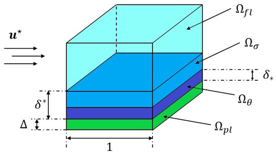
Figure 4. The homogenized continuum (from top to bottom): the viscous heat-conducting fluid ${\Omega }_{\mathrm{fl}}$, two thermoviscoelastic layers ${\Omega }_{\sigma }$ and ${\Omega }_{\theta }$, the thermoelastic layer (flat plate) ${\Omega }_{\mathrm{pl}}$.

The systems of Equations (40a)–(40d) and (40m)–(40p) governing, respectively, the behavior of the purely thermoelastic layer ${\Omega }_{\mathrm{pl}}$ and the purely thermoviscous layer ${\Omega }_{\mathrm{fl}}$ are classical. They are the same as the equations governing the continuums occupying, respectively, domains ${\Omega }_F^{\epsilon }$ and ${\Omega }_S^{\epsilon }$ in Model ${\mathrm{A}}_{\epsilon }$. The system of integro-differential equations with memory (40e)–(40h) governing the behavior of the thermoviscoelastic layer ${\Omega }_{\sigma }$, in principle, is also known in the literature. Up to the notation and change of sought functions, this system coincides with the system of homogenized equations of poroviscoelasticity with account of heat transfer, derived in Section 2.3 in [17] for macroscopic description of a highly viscous heat-conducting liquid filtering through a thermoelastic porous ground. In turn, the system of Equations (40i)–(40l) governing the behavior of the thermoviscoelastic layer ${\Omega }_{\theta }$ looks quite new and is unlikely to find direct analogues in the literature. The peculiarity of this system is the presence in Equations (40j) and (40k) of the unusual integrals with double convolution, which reflects the sophisticated memory effect due to the primary (i.e., before homogenization) presence of the three scales in the layer.

As has already been noted in the Introduction, Model H is a natural generalization of the macroscopic models built in [4,13]. In this regard, we can remark that Model H is an ‘enhanced’ version of the previous models in the following sense. If we discard in Model H all relations and constant and variable values directly related to heat transfer, then as a result, we obtain exactly the isothermal formulation built in [13]. Further, discarding layer ${\Omega }_{\theta }$ in the isothermal formulation followed by the proper matching of the interfacial conditions, we arrive exactly at the formulation built in [4].

As a matter of discussion, we can assume that the direct applications of Model H can relate to both qualitative and numerical analysis of the effective behavior of two-level bristly structures immersed in a liquid or gas. By qualitative analysis, here we mean the analysis of the form of homogenized coefficients in order to assess the contribution of certain physical characteristics of the microstructure to the macroscopic description of the continuum behavior and to clarify which thermomechanical effects are dominant.

As for numerical analysis, such an analysis is beyond the scope of the present article and is planned for the future. At the same time, based on the constructions made in Section 4 and Section 5 and in [13], we can now propose the following algorithm of determining the effective macroscopic physical characteristics, starting from the microstructure.

(i) 

Using the given data of the microstructure, solve Problems Z1–Z9 to find ${\mathit{Z}}_{00}^{ij}$, ${\mathit{Z}}_{10}^{ij}$, ${\mathit{Z}}_{20}$, ${\mathit{Z}}_{30}^{ij}$, ${\mathit{Z}}_{40}$, and $Z_5^i$; see [13] (pp. 1380–1383) and Appendix A.1 in Appendix A below.

(ii) 

Insert the solutions ${\mathit{Z}}_{00}^{ij}$, ${\mathit{Z}}_{10}^{ij}$, ${\mathit{Z}}_{20}$, ${\mathit{Z}}_{30}^{ij}$, ${\mathit{Z}}_{40}$, $Z_5^i$ into the representation of the homogenized two-scale coefficients that take place in Problems Y1–Y10. These representations are given by Formulas (7.14)–(7.23) from Section 7 in [13] and by Formulas (A6)–(A8) from Appendix A.2 in Appendix A.

(iii) 

Solve Problems Y1–Y10 to find ${\mathit{Y}}_0^{ij}$, ${\mathit{Y}}_1^{ij}$, ${\mathit{Y}}_2$, ${\mathit{Y}}_3^{ij}$, ${\mathit{Y}}_4$, ${\mathit{Y}}_5$, and $Y_6^i$ ($i,j=1,2,3$). The formulations of Problems Y1–Y7 are given in [13] (pp. 1411–1416). The formulations of Problems Y8–Y10 are given below in Appendix A.2 in Appendix A.

(iv) 

Insert the solutions of Problems Y1–Y10 into the representations of the homogenized macroscopic coefficients that take place in Model H. These representations are given by Formulas (12.2c–f) and (12.2h–l) from Section 12 in [13] and by the formulas from Appendix A.3 in Appendix A.

(v) 

Provided with the data obtained on the previous step, solve Problem H to find the macroscopic velocity distribution u and temperature distribution $\theta$.

This five-step algorithm is quite possible to implement numerically. Potentially, the presence of integrals with double convolution can lead to complication in numerical analysis, but what exactly such a complexity may be is unclear at this stage. The interim homogenized Model H-3sc is also worth consideration in line with a possible numerical analysis. In contrast, as we have noted before, Model ${\mathrm{A}}_{\epsilon }$ with a small $\epsilon$ is definitely inaccessible for practical analysis due to the enormous amount of necessary calculations.

From the point of view of promising applications in technology, as has been mentioned in the Introduction, Model H can most likely be useful in further modeling of airflow near the surface of a plant leaf, in modeling the epithelial surfaces of blood vessels, in modeling superhydrophobic and superoleophobic surfaces, as well as in designing biotechnological devices operating in liquids.

In future works, it would be useful and interesting to consider isothermal and non-isothermal Model ${\mathrm{A}}_{\epsilon }$-type systems taking into account transfer of admixture by a free flow of liquid (air) and sedimentation of the admixture particles on the surface of a two-level fine bristly structure. In such systems, the laws of balance of the admixture concentration in an open liquid (air) and on the solid–liquid (solid–air) interface can be taken in accordance with W. Hornung and W. Jaeger [18]. To homogenize the balance of the sedimented admixture on the solid–liquid (solid–air) interface, the Allaire–Damlamian–Hornung modified version of two-scale convergence [19] can be generalized and used. By this, one could make a further extension of the study of bristly structures in interaction with liquids and gases based on [13] and the present article.

Appendix A.1. The Cell Problems Posed on Θ

In (41), vector-function ${\mathit{Z}}_{40}={\mathit{Z}}_{40}(\widehat{\mathit{z}},x_3)$ vanishes for all $x_3\in (0,\Delta )\cup (\Delta +{\delta }_{*},1)$. On the segment $\{\Delta \le x_3\le \Delta +{\delta }_{*}\}$, vector-function ${\mathit{Z}}_{40}$ does not vary with change of $x_3$ and is the solution of the following cell problem:

Problem Z8.

Find a vector-function ${\mathit{Z}}_{40}={\mathit{Z}}_{40}\left(\widehat{\mathit{z}}\right)$, which satisfies the regularity condition

$${\mathit{Z}}_{40}\in {(H_{♯}^1(\Theta )/\mathbb{R})}^3,$$

(A1a)

and resolves the variational equations

$$\begin{array}{c}\hfill {\int }_{{\Theta }_F}\left(2{\alpha }_{\mu }{\mathbb{D}}_{\widehat{z}}\left({\mathit{Z}}_{40}\left(\widehat{\mathit{z}}\right)\right)+{\alpha }_{\lambda }\left({\mathrm{div}}_{\widehat{z}}{\mathit{Z}}_{40}\left(\widehat{\mathit{z}}\right)\right)\mathbb{I}-({\mathbb{B}}_F-{\mathbb{B}}_S)\right):{\nabla }_{\widehat{z}}{\mathit{\varphi }}_{21}\left(\widehat{\mathit{z}}\right)d\widehat{\mathit{z}}=0,\\ \hfill \forall {\mathit{\varphi }}_{21}\in H_{♯}^1{(\Theta )}^3,\end{array}$$

(A1b)

and

$$\begin{array}{c}\hfill {\int }_{{\Theta }_S}(\mathcal{G}:{\nabla }_{\widehat{z}}{\mathit{Z}}_{40}\left(\widehat{\mathit{z}}\right)):{\nabla }_{\widehat{z}}{\mathit{\varphi }}_{21}\left(\widehat{\mathit{z}}\right)d\widehat{\mathit{z}}+{\int }_{{\Theta }_F}{\alpha }_p\left({\mathrm{div}}_{\widehat{z}}{\mathit{Z}}_{40}\left(\widehat{\mathit{z}}\right)\right)\mathbb{I}:{\nabla }_{\widehat{z}}{\mathit{\varphi }}_{21}\left(\widehat{\mathit{z}}\right)d\widehat{\mathit{z}}=0,\\ \hfill \forall {\mathit{\varphi }}_{21}\in H_{♯}^1{(\Theta )}^3.\end{array}$$

(A1c)

In (42), scalar functions $Z_5^i$ ($i=1,2,3$) vanish for all $x_3\in (0,\Delta )\cup (\Delta +{\delta }_{*},1)$. On the segment $\{\Delta \le x_3\le \Delta +{\delta }_{*}\}$, scalar functions $Z_5^i$ do not vary with change of $x_3$ and are the solutions of the following cell problem:

Problem Z9.

Find a scalar function $\widehat{\mathit{z}}\mapsto Z_5^i(\widehat{\mathit{y}},\widehat{\mathit{z}})$ ($i=1,2,3$), which satisfies the regularity condition

$$Z_5^i(\widehat{\mathit{y}},·)\in H_{♯}^1(\Theta )/\mathbb{R},\widehat{\mathit{y}}\in \Sigma ,$$

(A2a)

and resolves the variational equation

$${\int }_{\Theta }(\widehat{\zeta }\left(\widehat{\mathit{y}}\right)\widehat{\psi }\left(\widehat{\mathit{z}}\right){\varkappa }_F+(1-\widehat{\zeta }\left(\widehat{\mathit{y}}\right)\widehat{\psi }\left(\widehat{\mathit{z}}\right)){\varkappa }_S)\left({\mathit{e}}_i+{\nabla }_{\widehat{\mathit{z}}}{Z}_5^i(\widehat{\mathit{y}},\widehat{\mathit{z}})\right)·{\nabla }_{\widehat{\mathit{z}}}{\eta }_{21}\left(\widehat{\mathit{z}}\right)d\widehat{\mathit{z}}=0,\forall {\eta }_{21}\in H_{♯}^1(\Theta ).$$

(A2b)

Variable $\widehat{\mathit{y}}$ plays the role of parameter in this formulation.

Problems Z8 and Z9 are well-posed. The proofs of their unique solvability are quite standard in the theory of generalized solutions to problems of mathematical physics, and therefore, we omit them here.

From a physical viewpoint, Equation (A1b) is the variational form of the Stokes equation of viscous compressible fluid and Equation (A1c) is the variational form of the classical linear elasticity equation. Since (A1b) contains matrices ${\mathbb{B}}_F$ and ${\mathbb{B}}_S$, Problem Z8 describes the stresses caused by the effect of thermal dilatation at the microscopic scale. In turn, Equation (A2b) is the variational heat equation and, correspondingly, Problem Z9 describes the heat transfer at the microscopic scale.

Appendix A.2. The Cell Problems Posed on Σ

In (43), vector-functions ${\mathit{Y}}_4={\mathit{Y}}_4(\widehat{\mathit{y}},x_3)$ and ${\mathit{Y}}_5={\mathit{Y}}_5(\widehat{\mathit{y}},x_3)$ vanish for all $x_3\in (0,\Delta )\cup (\Delta +{\delta }^{*},1)$. On the segment $\{\Delta \le x_3\le \Delta +{\delta }^{*}\}$, vector-functions ${\mathit{Y}}_4$ and ${\mathit{Y}}_5$ are the solutions of the following respective cell problems:

Problem Y8.

Find a vector-function $\widehat{\mathit{y}}\mapsto {\mathit{Y}}_4(\widehat{\mathit{y}},x_3)$ defined in the pattern cell $\Sigma$, which satisfies the regularity condition

$${\mathit{Y}}_4(·,x_3)\in {(H_{♯}^1(\Sigma )/\mathbb{R})}^3$$

(A3a)

and the integral equality

$${\int }_{\Sigma }\left[{\mathcal{A}}_0(\widehat{\mathit{y}},x_3):{\mathbb{D}}_{\widehat{\mathit{y}}}\left({\mathit{Y}}_4(\widehat{\mathit{y}},x_3)\right)+{\mathbb{H}}_{\theta 1}(\widehat{\mathit{y}},x_3)\right]:{\mathbb{D}}_{\widehat{y}}\left({\mathit{\varphi }}_{12}\left(\widehat{\mathit{y}}\right)\right)d\widehat{\mathit{y}}=0,\forall {\mathit{\varphi }}_{12}\in H_{♯}^1{(\Sigma )}^3.$$

(A3b)

Problem Y9.

Find a vector-function $(\widehat{\mathit{y}},t)\mapsto {\mathit{Y}}_5(\widehat{\mathit{y}},t,x_3)$, which satisfies the regularity condition

$${\mathit{Y}}_5(·,·,x_3)\in L^{\infty }(0,T;{(H_{♯}^1(\Sigma )/\mathbb{R})}^3)\cap H^1(0,T;H_{♯}^1{\left({\Sigma }_F\right)}^3),$$

(A4a)

and the integral equality

$$\begin{array}{cc}\hfill & {\int }_{\Sigma }[{\mathcal{A}}_0(\widehat{\mathit{y}},x_3):{\mathbb{D}}_{\widehat{y}}\left({\mathit{Y}}_5(\widehat{\mathit{y}},t,x_3)\right)+{\mathcal{B}}_0(\widehat{\mathit{y}},x_3):{\mathbb{D}}_{\widehat{y}}\left((J_t{\mathit{Y}}_5(\widehat{\mathit{y}},t,x_3)\right)\hfill \\ \hfill & +{\int }_0^t\left({\mathcal{A}}_1(\widehat{\mathit{y}},t-\tau ,x_3)+\left(J_t{\mathcal{B}}_1\right)(\widehat{\mathit{y}},t-\tau ,x_3)\right):{\mathbb{D}}_{\widehat{y}}\left({\mathit{Y}}_5(\widehat{\mathit{y}},\tau ,x_3)\right)d\tau \hfill \\ \hfill & +{\mathcal{B}}_0(\widehat{\mathit{y}},x_3):{\mathbb{D}}_{\widehat{y}}\left({\mathit{Y}}_4(\widehat{\mathit{y}},x_3)\right)+{\mathcal{A}}_1(\widehat{\mathit{y}},t,x_3):{\mathbb{D}}_{\widehat{y}}\left({\mathit{Y}}_4(\widehat{\mathit{y}},x_3)\right)\hfill \\ \hfill & +\left(J_t{\mathcal{B}}_1\right)(\widehat{\mathit{y}},t,x_3):{\mathbb{D}}_{\widehat{y}}\left({\mathit{Y}}_4\left(\widehat{\mathit{y}}\right)\right)+{\mathbb{H}}_{\theta 2}(\widehat{\mathit{y}},x_3)]:{\mathbb{D}}_{\widehat{y}}\left({\mathit{\varphi }}_{12}\left(\widehat{\mathit{y}}\right)\right)d\widehat{\mathit{y}}=0,\forall {\mathit{\varphi }}_{12}\in H_{♯}^1{(\Sigma )}^3,\hfill \end{array}$$

(A4b)

where ${\mathit{Y}}_4$ is the solution of Problem Y8.

In (44), scalar functions $Y_6^i=Y_6^i(\widehat{y},x_3)$ ($i=1,2,3$) vanish for all $x_3\in (0,\Delta )\cup (\Delta +{\delta }^{*},1)$. On the segment $\{\Delta \le x_3\le \Delta +{\delta }^{*}\}$, scalar functions $Y_6^i$ are the solutions of the following cell problem:

Problem Y10.

Find a scalar function $\widehat{\mathit{y}}\mapsto Y_6^i(·,x_3)$ ($i=1,2,3$) defined in the pattern cell $\Sigma$ for all $x_3\in [\Delta ,\Delta +{\delta }^{*}]$ and satisfying the regularity condition

$$Y_6^i(·,x_3)\in H_{♯}^1(\Sigma )/\mathbb{R},\forall x_3\in [\Delta ,\Delta +{\delta }^{*}],$$

(A5a)

and the integral equality

$${\int }_{\Sigma }{\mathbb{L}}_{\varkappa }(\widehat{\mathit{y}},x_3)\left(e_i+{\nabla }_{\widehat{\mathit{y}}}{Y}_6^i(\widehat{\mathit{y}},x_3)\right)·{\nabla }_{\widehat{\mathit{y}}}{\eta }_{12}\left(\widehat{\mathit{y}}\right)d\widehat{\mathit{y}}=0,\forall {\eta }_{12}\in H_{♯}^1(\Sigma ),\forall x_3\in [\Delta ,\Delta +{\delta }^{*}].$$

(A5b)

Variable $x_3$ enters the formulation of Problems Y8–Y10 parametrically. The fourth-rank tensors ${\mathcal{A}}_0$, ${\mathcal{A}}_1$, ${\mathcal{B}}_0$, and ${\mathcal{B}}_1$ and matrices ${\mathbb{H}}_{\theta 1}$, ${\mathbb{H}}_{\theta 2}$ and ${\mathbb{L}}_{\varkappa }$ in the formulations of Problems Y8–Y10 are uniquely defined by the microstructure and therefore are considered to be given. The exact form of tensors ${\mathcal{A}}_0$, ${\mathcal{A}}_1$, ${\mathcal{B}}_0$, and ${\mathcal{B}}_1$ on the segment $\{\Delta \le x_3\le \Delta +{\delta }^{*}\}$ can be found in [13] (pp. 1386–1387). Matrices ${\mathbb{H}}_{\theta 1}$, ${\mathbb{H}}_{\theta 2}$ and ${\mathbb{L}}_{\varkappa }$ are novel; they arise due to heat transfer and have the following form:

$${\mathbb{H}}_{\theta 1}(\widehat{\mathit{y}},x_3)=\left\{\begin{array}{c}{\displaystyle -\widehat{\zeta }(\widehat{\mathit{y}})\left(|{\Theta }_F|{\mathbb{B}}_F+(1-|{\Theta }_F|){\mathbb{B}}_S\right)\mathrm{for}{x}_3\in (\Delta +{\delta }_{*},\Delta +{\delta }^{*}],}\hfill \\ {\displaystyle \widehat{\zeta }(\widehat{\mathit{y}})[2{\alpha }_{\mu }{\int }_{\Theta }\widehat{\psi }(\widehat{\mathit{z}}){\mathbb{D}}_{\widehat{z}}({\mathit{Z}}_{40}(\widehat{\mathit{z}}))d\widehat{\mathit{z}}+{\alpha }_{\lambda }\left({\int }_{\Theta }\widehat{\psi }(\widehat{\mathit{z}}){\mathrm{div}}_{\widehat{z}}{\mathit{Z}}_{40}(\widehat{\mathit{z}})d\widehat{\mathit{z}}\right)\mathbb{I}}\hfill \\ -|{\Theta }_F|{\mathbb{B}}_F-(1-|{\Theta }_F|){\mathbb{B}}_S]\mathrm{for}{x}_3\in [\Delta ,\Delta +{\delta }_{*}],\hfill \end{array}\right.$$

(A6)

$${\mathbb{H}}_{\theta 2}(\widehat{\mathit{y}},x_3)=\left\{\begin{array}{c}{\displaystyle 0\mathrm{for}{x}_3\in (\Delta +{\delta }_{*},\Delta +{\delta }^{*}],}\hfill \\ {\displaystyle \widehat{\zeta }(\widehat{\mathit{y}})\left[{\alpha }_p\left({\int }_{\Theta }\widehat{\psi }(\widehat{\mathit{z}}){\mathrm{div}}_{\widehat{z}}{\mathit{Z}}_{40}(\widehat{\mathit{z}})d\widehat{\mathit{z}}\right)\mathbb{I}+\mathcal{G}:{\int }_{\Theta }(1-\widehat{\psi }(\widehat{\mathit{z}})){\nabla }_{\widehat{z}}{\mathit{Z}}_{40}(\widehat{\mathit{z}})d\widehat{\mathit{z}}\right]}\hfill \\ \mathrm{for}{x}_3\in [\Delta ,\Delta +{\delta }_{*}],\hfill \end{array}\right.$$

(A7)

$${\mathbb{L}}_{\varkappa }(\widehat{\mathit{y}},x_3)=\left\{\begin{array}{c}{\displaystyle \left(\widehat{\zeta }(\widehat{\mathit{y}}){\varkappa }_F+(1-\widehat{\zeta }(\widehat{\mathit{y}})){\varkappa }_S\right)\mathbb{I}\mathrm{for}{x}_3\in (\Delta +{\delta }_{*},\Delta +{\delta }^{*}],}\hfill \\ {\displaystyle (\widehat{\zeta }(\widehat{\mathit{y}})\left|{\Theta }_F\right|{\varkappa }_F+\left(1-\widehat{\zeta }(\widehat{\mathit{y}})\left|{\Theta }_F\right|\right){\varkappa }_S)\mathbb{I}}\hfill \\ {\displaystyle +\widehat{\zeta }(\widehat{\mathit{y}})({\varkappa }_F-{\varkappa }_S){\int }_{\Theta }\widehat{\psi }(\widehat{\mathit{z}}){\nabla }_{\widehat{z}}\left(\sum _{i=1}^3{Z}_5^i(\widehat{\mathit{y}},\widehat{\mathit{z}}){\mathit{e}}_i\right)d\widehat{\mathit{z}}\mathrm{for} x_3\in [\Delta ,\Delta +{\delta }_{*}].}\hfill \end{array}\right.$$

(A8)

In the last expression, by ${\mathit{e}}_i$ ($i=1,2,3$) the standard vectors of Cartesian basis in ${\mathbb{R}}^3$ are denoted.

Remark A1.

Note that ${\mathit{Y}}_4$, ${\mathit{Y}}_5$, and ${\mathit{Y}}_6^i$ do not vary with change of $x_3$ on each of the segments $\{\Delta <x_3<\Delta +{\delta }_{*}\}$ and $\{\Delta +{\delta }_{*}<x_3<\Delta +{\delta }^{*}\}$, since the coefficients in Equations (A3b), (A4b), and (A5b) do not vary with change of $x_3$ on these segments.

Problems Y8–Y10 are well-posed. The proofs of their unique solvability are quite standard in the theory of generalized solutions to boundary value problems of partial differential equations, and therefore, we omit them here.

From a physical viewpoint, if we carefully trace the origin of the averaged coefficients in variational Equations (A3b) and (A4b), then we can see that Problems Y8 and Y9 describe the homogenized stresses caused by the effect of thermal dilatation at the mesoscopic scale. In turn, Equation (A5b) is the variational form of homogenized heat equation and, correspondingly, Problem Y10 describes the homogenized heat transfer at the mesoscopic scale.

Appendix A.3. Representations of Effective Coefficients

Tensors ${\mathcal{P}}^{\sigma }$, ${\mathcal{G}}^{\sigma }$, ${\mathcal{R}}_0^{\sigma }$, ${\mathcal{F}}_v^{\sigma }$, ${\mathcal{P}}^{\theta }$, ${\mathcal{G}}^{\theta }$, ${\mathcal{R}}_1^{\theta }$, ${\mathcal{R}}_2^{\theta }$, and ${\mathcal{F}}_v^{\theta }$ and matrices ${\mathbb{F}}_p^{\sigma }$ and ${\mathbb{F}}_p^{\theta }$ are not related to heat transfer and have already been established earlier; see Formulas (12.2c–f) and (12.2h–l) from [13]. The procedure of derivation of the rest of effective macroscopic characteristics in Model H is described in the proof of Theorem 2.

To present these effective characteristics, we further use the following notation:

Notation A1.

The $3\times 3$-matrix ${\mathbb{J}}^{mn}$ ($m,n=1,2,3$) is defined by the formula

$${\mathbb{J}}^{mn}={\displaystyle \frac{{\mathit{e}}_m\otimes {\mathit{e}}_n+{\mathit{e}}_n\otimes {\mathit{e}}_m}{2}},$$

or, in the component-wise form,

$${({\mathbb{J}}^{mn})}_{ij}={\displaystyle \frac{{\delta }_{im}{\delta }_{jn}+{\delta }_{jm}{\delta }_{in}}{2}},i,j=1,2,3.$$

With account of this notation, we write down the representations as follows:

$$\begin{array}{cc}\hfill {\mathbb{V}}^{\sigma }=& {\alpha }_{\lambda }\mathbb{I}{\int }_{\Sigma }\widehat{\zeta }(\widehat{\mathit{y}}){\mathrm{div}}_{\widehat{y}}{\mathit{Y}}_4(\widehat{\mathit{y}},x_3)d\widehat{\mathit{y}}+2{\alpha }_{\mu }{\int }_{\Sigma }\widehat{\zeta }(\widehat{\mathit{y}}){\mathbb{D}}_{\widehat{y}}({\mathit{Y}}_4(\widehat{\mathit{y}},x_3))d\widehat{\mathit{y}},\hfill \\ \hfill {\mathbb{E}}^{\sigma }=& {\alpha }_p\mathbb{I}{\int }_{\Sigma }\widehat{\zeta }(\widehat{\mathit{y}}){\mathrm{div}}_{\widehat{y}}{\mathit{Y}}_4(\widehat{\mathit{y}},x_3)d\widehat{\mathit{y}}+\mathcal{G}:{\int }_{\Sigma }(1-\widehat{\zeta }(\widehat{\mathit{y}})){\mathbb{D}}_{\widehat{y}}({\mathit{Y}}_4(\widehat{\mathit{y}},x_3))d\widehat{\mathit{y}},\hfill \\ \hfill {\mathbb{R}}_1^{\sigma }(t)=& {\alpha }_{\lambda }\mathbb{I}{\int }_{\Sigma }\widehat{\zeta }(\widehat{\mathit{y}}){\mathrm{div}}_{\widehat{y}}{\mathit{Y}}_5(\widehat{\mathit{y}},t,x_3)d\widehat{\mathit{y}}+2{\alpha }_{\mu }{\int }_{\Sigma }\widehat{\zeta }(\widehat{\mathit{y}}){\mathbb{D}}_{\widehat{y}}({\mathit{Y}}_5(\widehat{\mathit{y}},t,x_3))d\widehat{\mathit{y}}\hfill \\ \hfill & +{\alpha }_p\mathbb{I}{\int }_0^t{\int }_{\Sigma }\widehat{\zeta }(\widehat{\mathit{y}}){\mathrm{div}}_{\widehat{y}}{\mathit{Y}}_5(\widehat{\mathit{y}},t^{\prime },x_3)d\widehat{\mathit{y}}d{t}^{\prime }\hfill \\ \hfill & +\mathcal{G}:{\int }_0^t{\int }_{\Sigma }(1-\widehat{\zeta }(\widehat{\mathit{y}})){\mathbb{D}}_{\widehat{y}}({\mathit{Y}}_5(\widehat{\mathit{y}},t^{\prime },x_3))d\widehat{\mathit{y}}d{t}^{\prime },\hfill \\ \hfill {\mathbb{L}}_{*}^{\sigma }=& \left(|{\Sigma }_F|{\varkappa }_F+(1-|{\Sigma }_F|){\varkappa }_S\right)\mathbb{I}+({\varkappa }_F-{\varkappa }_S){\left[{\int }_{\Sigma }\widehat{\zeta }(\widehat{\mathit{y}}){\nabla }_{\widehat{y}}\left(\sum _{i=1}^3{Y}_{\mathit{6}}(\widehat{\mathit{y}},x_3){\mathit{e}}_i\right)d\widehat{\mathit{y}}\right]}^{tr},\hfill \\ \hfill {\mathbb{L}}_{B3}^{\sigma }=& |{\Sigma }_F|{\mathbb{B}}_F+(1-|{\Sigma }_F|){\mathbb{B}}_S+\sum _{i,j=1}^3{\mathbb{J}}^{ij}\left(({\mathbb{B}}_F-{\mathbb{B}}_S):{\int }_{\Sigma }\widehat{\zeta }(\widehat{\mathit{y}}){\mathbb{D}}_{\widehat{y}}(Y_{\mathit{0}}^{ij}(\widehat{\mathit{y}},x_3))d\widehat{\mathit{y}}\right),\hfill \\ \hfill {\mathbb{L}}_{B4}^{\sigma }(t)=& \sum _{i,j=1}^3{\mathbb{J}}^{ij}\left(({\mathbb{B}}_F-{\mathbb{B}}_S):{\int }_{\Sigma }\widehat{\zeta }(\widehat{\mathit{y}}){\mathbb{D}}_{\widehat{y}}({\mathit{Y}}_1^{ij}(\widehat{\mathit{y}},t,x_3))d\widehat{\mathit{y}}\right),\hfill \\ \hfill {\mathbb{L}}_v^{\star \sigma }(t)=& \sum _{i,j=1}^3{\mathbb{J}}^{ij}\left(({\mathbb{B}}_F-{\mathbb{B}}_S):{\int }_{\Sigma }\widehat{\zeta }(\widehat{y}){\mathbb{D}}_{\widehat{y}}(Y_3^{ij}(\widehat{y},t,x_3))d\widehat{y}\right),\hfill \\ \hfill L_{\theta 1}^{\sigma }=& ({\mathbb{B}}_F-{\mathbb{B}}_S):{\int }_{\Sigma }\widehat{\zeta }(\widehat{\mathit{y}}){\mathbb{D}}_{\widehat{y}}({\mathit{Y}}_4(\widehat{\mathit{y}},x_3))d\widehat{\mathit{y}},\hfill \\ \hfill L_{\theta 2}^{\sigma }(t)=& ({\mathbb{B}}_F-{\mathbb{B}}_S):{\int }_{\Sigma }\widehat{\zeta }(\widehat{\mathit{y}}){\mathbb{D}}_{\widehat{y}}({\mathit{Y}}_5(\widehat{\mathit{y}},t,x_3))d\widehat{\mathit{y}},\hfill \\ \hfill L_p^{\star \sigma }(t)=& ({\mathbb{B}}_F-{\mathbb{B}}_S):{\int }_{\Sigma }\widehat{\zeta }(\widehat{\mathit{y}}){\mathbb{D}}_{\widehat{y}}({\mathit{Y}}_2(\widehat{\mathit{y}},t,x_3))d\widehat{\mathit{y}}\hfill \end{array}$$

for $x_3\in (\Delta +{\delta }_{*},\Delta +{\delta }^{*}]$,

$$\begin{array}{cc}\hfill {\mathbb{V}}^{\theta }=& {\int }_{\Sigma }\left[{\mathcal{A}}_0(\widehat{\mathit{y}},x_3):{\mathbb{D}}_{\widehat{\mathit{y}}}({\mathit{Y}}_4(\widehat{\mathit{y}},x_3))+{\mathbb{H}}_{\theta 1}(\widehat{\mathit{y}},x_3)\right]d\widehat{\mathit{y}},\hfill \\ \hfill {\mathbb{E}}^{\theta }=& {\int }_{\Sigma }\left[{\mathcal{B}}_0(\widehat{\mathit{y}},x_3):{\mathbb{D}}_{\widehat{y}}({\mathit{Y}}_4(\widehat{\mathit{y}},x_3))+{\mathbb{H}}_{\theta 2}(\widehat{\mathit{y}},x_3)\right]d\widehat{\mathit{y}},\hfill \\ \hfill {\mathbb{R}}_1^{\theta }(t)=& {\int }_{\Sigma }\left[{\mathcal{A}}_0(\widehat{\mathit{y}},x_3):{\mathbb{D}}_{\widehat{y}}({\mathit{Y}}_5(\widehat{\mathit{y}},t,x_3))+{\mathcal{A}}_1(\widehat{\mathit{y}},t,x_3):{\mathbb{D}}_{\widehat{y}}({\mathit{Y}}_4(\widehat{\mathit{y}},x_3))\right]d\widehat{\mathit{y}}\hfill \\ \hfill & +{\int }_0^t{\int }_{\Sigma }\left[{\mathcal{B}}_0(\widehat{\mathit{y}},x_3):{\mathbb{D}}_{\widehat{y}}({\mathit{Y}}_5(\widehat{\mathit{y}},t^{\prime },x_3))+{\mathcal{B}}_1(\widehat{\mathit{y}},t^{\prime },x_3):{\mathbb{D}}_{\widehat{y}}({\mathit{Y}}_4(\widehat{\mathit{y}},x_3))\right]d\widehat{\mathit{y}}d{t}^{\prime },\hfill \\ \hfill {\mathbb{R}}_2^{\theta }(t_1,t_2)=& {\int }_{\Sigma }{\mathcal{A}}_1(\widehat{\mathit{y}},t_1,x_3):{\mathbb{D}}_{\widehat{y}}({\mathit{Y}}_5(\widehat{\mathit{y}},t_2,x_3))]d\widehat{\mathit{y}}\hfill \\ \hfill & +{\int }_0^{t_2}{\int }_{\Sigma }{\mathcal{B}}_1(\widehat{\mathit{y}},t_1,x_3):{\mathbb{D}}_{\widehat{y}}({\mathit{Y}}_5(\widehat{\mathit{y}},t_2^{\prime },x_3))]d\widehat{\mathit{y}}d{t}_2^{\prime },\hfill \\ \hfill {\mathbb{L}}_{*}^{\theta }=& {\int }_{\Sigma }{\mathbb{L}}_{\varkappa }(\widehat{\mathit{y}},x_3)\left(\mathbb{I}+{\left[{\nabla }_{\widehat{y}}\sum _{i=1}^3{Y}_{\mathit{6}}(\widehat{\mathit{y}},x_3){\mathit{e}}_i\right]}^{tr}\right)d\widehat{\mathit{y}},\hfill \\ \hfill {\mathbb{L}}_{B3}^{\theta }=& |{\Sigma }_F\left|\right|{\Theta }_F|{\mathbb{B}}_F+(1-|{\Sigma }_F\left|\right|{\Theta }_F|){\mathbb{B}}_S\hfill \\ \hfill & +|{\Sigma }_F|\sum _{i,j=1}^3{\mathbb{J}}^{ij}\left(({\mathbb{B}}_F-{\mathbb{B}}_S):{\int }_{\Theta }\widehat{\psi }(\widehat{z}){\mathbb{D}}_{\widehat{z}}({\mathit{Z}}_{00}^{ij}(\widehat{\mathit{z}},x_3))d\widehat{\mathit{z}}\right)\hfill \\ \hfill & +\sum _{i,j=1}^3{\mathbb{J}}^{ij}\left(|{\Theta }_F|({\mathbb{B}}_F-{\mathbb{B}}_S):{\int }_{\Sigma }\widehat{\zeta }(\widehat{\mathit{y}}){\mathbb{D}}_{\widehat{y}}({\mathit{Y}}_0^{ij}(\widehat{\mathit{y}},x_3))d\widehat{\mathit{y}}\right)\hfill \\ \hfill & +\sum _{i,j=1}^3{\mathbb{J}}^{ij}(\sum _{m,n=1}^3\left[{\mathbb{J}}^{mn}\left(({\mathbb{B}}_F-{\mathbb{B}}_S):{\int }_{\Theta }\widehat{\psi }(\widehat{\mathit{z}}){\mathbb{D}}_{\widehat{z}}({\mathit{Z}}_{00}^{mn}(\widehat{\mathit{z}},x_3))d\widehat{\mathit{z}}\right)\right]\hfill \\ \hfill & :{\int }_{\Sigma }\widehat{\zeta }(\widehat{\mathit{y}}){\mathbb{D}}_{\widehat{y}}({\mathit{Y}}_0^{ij}(\widehat{\mathit{y}},x_3))d\widehat{\mathit{y}}),\hfill \\ \hfill {\mathbb{L}}_{B4}^{\theta }(t)=& \sum _{i,j=1}^3{\mathbb{J}}^{ij}\left(|{\Theta }_F|({\mathbb{B}}_F-{\mathbb{B}}_S):{\int }_{\Sigma }\widehat{\zeta }(\widehat{\mathit{y}}){\mathbb{D}}_{\widehat{y}}({\mathit{Y}}_1^{ij}(\widehat{\mathit{y}},t,x_3))d\widehat{\mathit{y}}\right)\hfill \\ \hfill & +\sum _{i,j=1}^3{\mathbb{J}}^{ij}(\sum _{m,n=1}^3\left[{\mathbb{J}}^{mn}\left(({\mathbb{B}}_F-{\mathbb{B}}_S):{\int }_{\Theta }\widehat{\psi }(\widehat{\mathit{z}}){\mathbb{D}}_{\widehat{z}}({\mathit{Z}}_{00}^{mn}(\widehat{\mathit{z}},x_3))d\widehat{\mathit{z}}\right)\right]\hfill \\ \hfill & :{\int }_{\Sigma }\widehat{\zeta }(\widehat{\mathit{y}}){\mathbb{D}}_{\widehat{y}}({\mathit{Y}}_1^{ij}(\widehat{\mathit{y}},t,x_3))d\widehat{\mathit{y}})\hfill \\ \hfill & +|{\Sigma }_F|\sum _{i,j=1}^3{\mathbb{J}}^{ij}\left(({\mathbb{B}}_F-{\mathbb{B}}_S):{\int }_{\Theta }\widehat{\psi }(\widehat{\mathit{z}}){\mathbb{D}}_{\widehat{z}}({\mathit{Z}}_{10}^{ij}(\widehat{\mathit{z}},t,x_3))d\widehat{\mathit{z}}\right)\hfill \\ \hfill & +\sum _{i,j=1}^3{\mathbb{J}}^{ij}(\sum _{m,n=1}^3\left[{\mathbb{J}}^{mn}\left(({\mathbb{B}}_F-{\mathbb{B}}_S):{\int }_{\Theta }\widehat{\psi }(\widehat{\mathit{z}}){\mathbb{D}}_{\widehat{z}}({\mathit{Z}}_{10}^{mn}(\widehat{\mathit{z}},t,x_3))d\widehat{\mathit{z}}\right)\right]\hfill \\ \hfill & :{\int }_{\Sigma }\widehat{\zeta }(\widehat{\mathit{y}}){\mathbb{D}}_{\widehat{y}}({\mathit{Y}}_0^{ij}(\widehat{\mathit{y}},x_3))d\widehat{\mathit{y}}),\hfill \\ \hfill {\mathbb{L}}_{B5}^{\theta }(t_1,t_2)=& \sum _{i,j=1}^3{\mathbb{J}}^{ij}(\sum _{m,n=1}^3\left[{\mathbb{J}}^{mn}\left(({\mathbb{B}}_F-{\mathbb{B}}_S):{\int }_{\Theta }\widehat{\psi }(\widehat{\mathit{z}}){\mathbb{D}}_{\widehat{z}}({\mathit{Z}}_{10}^{mn}(\widehat{\mathit{z}},t_1,x_3))d\widehat{\mathit{z}}\right)\right]\hfill \\ \hfill & :{\int }_{\Sigma }\widehat{\zeta }(\widehat{\mathit{y}}){\mathbb{D}}_{\widehat{y}}({\mathit{Y}}_1^{ij}(\widehat{\mathit{y}},t_2,x_3))d\widehat{\mathit{y}}),\hfill \\ \hfill {\mathbb{L}}_v^{\star \theta }(t)=& \sum _{i,j=1}^3{\mathbb{J}}^{ij}\left(|{\Theta }_F|({\mathbb{B}}_F-{\mathbb{B}}_S):{\int }_{\Sigma }\widehat{\zeta }(\widehat{\mathit{y}}){\mathbb{D}}_{\widehat{y}}({\mathit{Y}}_3^{ij}(\widehat{\mathit{y}},t,x_3))d\widehat{\mathit{y}}\right)\hfill \\ \hfill & +\sum _{i,j=1}^3{\mathbb{J}}^{ij}(\sum _{m,n=1}^3\left[{\mathbb{J}}^{mn}\left(({\mathbb{B}}_F-{\mathbb{B}}_S):{\int }_{\Theta }\widehat{\psi }(\widehat{\mathit{z}}){\mathbb{D}}_{\widehat{z}}({\mathit{Z}}_{00}^{mn}(\widehat{\mathit{z}},x_3))d\widehat{\mathit{z}}\right)\right]\hfill \\ \hfill & :{\int }_{\Sigma }\widehat{\zeta }(\widehat{\mathit{y}}){\mathbb{D}}_{\widehat{y}}({\mathit{Y}}_3^{ij}(\widehat{\mathit{y}},t,x_3))d\widehat{\mathit{y}})\hfill \\ \hfill & +{\int }_0^t\sum _{i,j=1}^3{\mathbb{J}}^{ij}(\sum _{m,n=1}^3\left[{\mathbb{J}}^{mn}\left(({\mathbb{B}}_F-{\mathbb{B}}_S):{\int }_{\Theta }\widehat{\psi }(\widehat{\mathit{z}}){\mathbb{D}}_{\widehat{z}}({\mathit{Z}}_{10}^{mn}(\widehat{\mathit{z}},t-t^{\prime },x_3))d\widehat{\mathit{z}}\right)\right]\hfill \\ \hfill & :{\int }_{\Sigma }\widehat{\zeta }(\widehat{\mathit{y}}){\mathbb{D}}_{\widehat{y}}({\mathit{Y}}_3^{ij}(\widehat{\mathit{y}},t^{\prime },x_3))d\widehat{\mathit{y}})d{t}^{\prime },\hfill \\ \hfill L_{\theta 1}^{\theta }=& (|{\Theta }_F|({\mathbb{B}}_F-{\mathbb{B}}_S):{\int }_{\Sigma }\widehat{\zeta }(\widehat{\mathit{y}}){\mathbb{D}}_{\widehat{y}}({\mathit{Y}}_4(\widehat{\mathit{y}},x_3))d\widehat{\mathit{y}}\hfill \\ \hfill & +\sum _{i,j=1}^3\left[{\mathbb{J}}^{mn}\left(({\mathbb{B}}_F-{\mathbb{B}}_S):{\int }_{\Theta }\widehat{\psi }(\widehat{\mathit{z}}){\mathbb{D}}_{\widehat{z}}({\mathit{Z}}_{00}^{ij}(\widehat{\mathit{z}},x_3))d\widehat{\mathit{z}}\right)\right]\hfill \\ \hfill & :{\int }_{\Sigma }\widehat{\zeta }(\widehat{\mathit{y}}){\mathbb{D}}_{\widehat{y}}({\mathit{Y}}_4(\widehat{\mathit{y}},x_3))d\widehat{\mathit{y}}\hfill \\ \hfill & +|{\Sigma }_F|({\mathbb{B}}_F-{\mathbb{B}}_S):{\int }_{\Theta }\widehat{\psi }(\widehat{z}){\mathbb{D}}_{\widehat{z}}({\mathit{Z}}_{40}(\widehat{\mathit{z}}))d\widehat{\mathit{z}},\hfill \\ \hfill L_p^{\star \theta }(t)=& (|{\Theta }_F|({\mathbb{B}}_F-{\mathbb{B}}_S):{\int }_{\Sigma }\widehat{\zeta }(\widehat{\mathit{y}}){\mathbb{D}}_{\widehat{y}}({\mathit{Y}}_2(\widehat{\mathit{y}},t,x_3))d\widehat{\mathit{y}}\hfill \\ \hfill & +\sum _{i,j=1}^3\left[{\mathbb{J}}^{ij}\left(({\mathbb{B}}_F-{\mathbb{B}}_S):{\int }_{\Theta }\widehat{\psi }(\widehat{z}){\mathbb{D}}_{\widehat{z}}({\mathit{Z}}_{00}^{ij}(\widehat{\mathit{z}},x_3))d\widehat{\mathit{z}}\right)\right]\hfill \\ \hfill & :{\int }_{\Sigma }\widehat{\zeta }(\widehat{\mathit{y}}){\mathbb{D}}_{\widehat{y}}(Y_{\mathit{2}}(\widehat{\mathit{y}},t,x_3))d\widehat{\mathit{y}}\hfill \\ \hfill & +{\int }_0^t\sum _{i,j=1}^3\left[{\mathbb{J}}^{ij}\left(({\mathbb{B}}_F-{\mathbb{B}}_S):{\int }_{\Theta }\widehat{\psi }(\widehat{\mathit{z}}){\mathbb{D}}_{\widehat{z}}({\mathit{Z}}_{10}^{ij}(\widehat{z},t-t^{\prime },x_3))d\widehat{\mathit{z}}\right)\right]\hfill \\ \hfill & :{\int }_{\Sigma }\widehat{\zeta }(\widehat{\mathit{y}}){\mathbb{D}}_{\widehat{y}}({\mathit{Y}}_2(\widehat{\mathit{y}},t^{\prime },x_3))d\widehat{\mathit{y}}d{t}^{\prime },\hfill \\ \hfill L_{\theta 2}^{\theta }(t)=& (|{\Theta }_F|({\mathbb{B}}_F-{\mathbb{B}}_S):{\int }_{\Sigma }\widehat{\zeta }(\widehat{\mathit{y}}){\mathbb{D}}_{\widehat{y}}({\mathit{Y}}_5(\widehat{\mathit{y}},t,x_3))d\widehat{\mathit{y}}\hfill \\ \hfill & +\sum _{i,j=1}^3\left[{\mathbb{J}}^{ij}\left(({\mathbb{B}}_F-{\mathbb{B}}_S):{\int }_{\Theta }\widehat{\psi }(\widehat{z}){\mathbb{D}}_{\widehat{z}}({\mathit{Z}}_{00}^{ij}(\widehat{\mathit{z}},x_3))d\widehat{\mathit{z}}\right)\right]\hfill \\ \hfill & :{\int }_{\Sigma }\widehat{\zeta }(\widehat{\mathit{y}}){\mathbb{D}}_{\widehat{y}}({\mathit{Y}}_5(\widehat{\mathit{y}},t,x_3))d\widehat{\mathit{y}}\hfill \\ \hfill & +\sum _{i,j=1}^3\left[{\mathbb{J}}^{ij}\left(({\mathbb{B}}_F-{\mathbb{B}}_S):{\int }_{\Theta }\widehat{\psi }(\widehat{\mathit{z}}){\mathbb{D}}_{\widehat{z}}({\mathit{Z}}_{10}^{ij}(\widehat{\mathit{z}},t,x_3))d\widehat{\mathit{z}}\right)\right]\hfill \\ \hfill & :{\int }_{\Sigma }\widehat{\zeta }(\widehat{\mathit{y}}){\mathbb{D}}_{\widehat{y}}({\mathit{Y}}_4(\widehat{\mathit{y}},x_3))d\widehat{\mathit{y}},\hfill \\ \hfill L_{\theta 3}^{\theta }(t_1,t_2)=& \sum _{i,j=1}^3\left[{\mathbb{J}}^{ij}\left(({\mathbb{B}}_F-{\mathbb{B}}_S):{\int }_{\Theta }\widehat{\psi }(\widehat{\mathit{z}}){\mathbb{D}}_{\widehat{z}}({\mathit{Z}}_{10}^{ij}(\widehat{\mathit{z}},t_1,x_3))d\widehat{\mathit{z}}\right)\right]\hfill \\ \hfill & :{\int }_{\Sigma }\widehat{\zeta }(\widehat{\mathit{y}}){\mathbb{D}}_{\widehat{y}}({\mathit{Y}}_5(\widehat{\mathit{y}},t_2,x_3))d\widehat{\mathit{y}}\hfill \end{array}$$

for $x_3\in [\Delta ,\Delta +{\delta }_{*}]$.

Note that all these matrices and scalars do not depend on $x_3$, in fact, due to Remark A1 and Remarks 17 and 25 from [13].

References

- Goldstein, S. Modern Developments in Fluid Dynamics. An Account of Theory and Experiment Relating to Boundary Layers, Turbulent Motion and Wakes. Volume I; Clarendon Press: Oxford, UK, 1938. [Google Scholar]
- Schreuder, M.D.J.; Brewer, C.A.; Heine, C. Modelled influences of non-exchanging trichomes on leaf boundary layers and gas exchange. J. Theor. Biol. 2001, 210, 23–32. [Google Scholar] [CrossRef]
- Vogel, S. Life in Moving Fluids: The Physical Biology of Flow, 2nd ed.; Pinceton University Press: Princeton, NJ, USA, 1994. [Google Scholar]
- Hoffmann, K.-H.; Botkin, N.D.; Starovoitov, V.N. Homogenization of interfaces between rapidly oscillating fine elastic structures and fluids. SIAM J. Appl. Math. 2005, 65, 983–1005. [Google Scholar] [CrossRef]
- Botkin, N.D.; Hoffmann, K.-H.; Pykhteev, O.A.; Turova, V.L. Dispersion relations for acoustic waves in heterogeneous multi-layered structures contacting with fluids. J. Frankl. Inst. 2007, 344, 520–534. [Google Scholar] [CrossRef][Green Version]
- Botkin, N.; Turova, V. Simulation of acoustic wave propagation in anisotropic media using dynamic programming technique. In System Modeling and Optimization. CSMO 2013. IFIP Advances in Information and Communication Technology, Volume 443; Pötzsche, C., Heuberger, C., Kaltenbacher, B., Rendl, F., Eds.; Springer: Berlin/Heidelberg, Germany, 2014; pp. 36–51. [Google Scholar]
- Turova, V.; Kovtanyuk, A.; Pykhteev, O.; Sidorenko, I.; Lampe, R. Glycocalyx sensing with a mathematical model of acoustic shear wave biosensor. Bioengineering 2022, 9, 462. [Google Scholar] [CrossRef]
- Genaev, M.A.; Doroshkov, A.V.; Pshenichnikova, T.A.; Kolchanov, N.I.; Afonnikov, D.A. Extraction of quantitative characteristics describing wheat leaf pubescence with a novel image-processing technique. Planta 2012, 236, 1943–1954. [Google Scholar] [CrossRef]
- Pomeranz, M.; Campbell, J.; Siegal-Gaskins, D.; Engelmeier, J.; Wilson, T.; Fernandez, V.; Brkljacic, J.; Grotewold, E. High-resolution computational imaging of leaf hair patterning using polarized light microscopy. Plant J. 2013, 73, 701–708. [Google Scholar] [CrossRef]
- Pshenichnikova, T.A.; Doroshkov, A.V.; Osipova, S.V.; Permyakov, A.V.; Permyakova, M.D.; Efimov, V.M.; Afonnikov, D.A. Quantitative characteristics of pubescence in wheat (Triticum aestivum L.) are associated with photosynthetic parameters under conditions of normal and limited water supply. Planta 2019, 249, 839–847. [Google Scholar] [CrossRef]
- Koch, K.; Bhushan, B.; Barthlott, W. Multifunctional plant surfaces and smart materials. In Springer Handbook of Nanotechnology, Part F: Biomimetics; Bhushan, B., Ed.; Springer: Berlin/Heidelberg, Germany, 2010; pp. 1399–1436. [Google Scholar]
- Bhushan, B.; Jung, Y.C.; Nosonovsky, M. Lotus effect: Surfaces with roughness-induced superhydrophobicity, self-cleaning and low adhesion. In Springer Handbook of Nanotechnology, Part F: Biomimetics; Bhushan, B., Ed.; Springer: Berlin/Heidelberg, Germany, 2010; pp. 1437–1524. [Google Scholar]
- Sazhenkov, S.A.; Sazhenkova, E.V. Homogenization of a submerged two-level bristle structure for modeling in biotechnology. Sib. Élektron. Mat. Izv. 2020, 17, 1359–1450. [Google Scholar] [CrossRef]
- Allaire, G.; Briane, M. Multiscale convergence and reiterated homogenization. Proc. R. Soc. Edinb. 1996, 126A, 298–341. [Google Scholar]
- Meirmanov, A.M.; Sazhenkov, S.A. Generalized solutions to linearized equations of thermoelastic solid viscous thermofluid. Electron. J. Differ. Equ. 2007, 2007, 41. [Google Scholar]
- Oleinik, O.A.; Shamaev, A.S.; Yosifian, G.A. Mathematical Problems in Elasticity and Homogenization; North-Holland: Amsterdam, The Netherlands, 1992. [Google Scholar]
- Meirmanov, A.M. Mathematical Models for Poroelastic Flows; Atlantis Press: Amsterdam, The Netherlands, 2014. [Google Scholar]
- Hornung, U.; Jäger, W. Diffusion, convection, adsorption and reaction of chemicals in porous media. J. Differ. Equ. 1991, 92, 199–225. [Google Scholar] [CrossRef]
- Allaire, G.; Damlamian, A.; Hornung, U. Two-scale convergence on periodic surfaces and applications. In Proceedings of the International Conference on Mathematical Modelling of Flow through Porous Media (May 1995); Bourgeat, A., Carasso, C., Luckhaus, S., Mikelić, A., Eds.; World Scientific Publishing Co.: Singapore, 1996; pp. 15–25. [Google Scholar]
Disclaimer/Publisher’s Note: The statements, opinions and data contained in all publications are solely those of the individual author(s) and contributor(s) and not of MDPI and/or the editor(s). MDPI and/or the editor(s) disclaim responsibility for any injury to people or property resulting from any ideas, methods, instructions or products referred to in the content. |
© 2024 by the authors. Licensee MDPI, Basel, Switzerland. This article is an open access article distributed under the terms and conditions of the Creative Commons Attribution (CC BY) license (https://creativecommons.org/licenses/by/4.0/).