Stability of Certain Non-Autonomous Cooperative Systems of Difference Equations with the Application to Evolutionary Dynamics

Abstract

This paper investigates the dynamics of non-autonomous cooperative systems of difference equations with asymptotically constant coefficients. We are mainly interested in global attractivity results for such systems and the application of such results to evolutionary population cooperation models. We use two methods to extend the global attractivity results for autonomous cooperative systems to related non-autonomous cooperative systems which appear in recent problems in evolutionary dynamics.

1. Introduction and Preliminaries

In this paper, we give some global attractivity results for a non-autonomous cooperative systems of difference equations

$$\begin{array}{ccc}\hfill x_{n+1}& =& {\displaystyle a_{n}f(x_n,y_n)}\hfill \\ \hfill y_{n+1}& =& {\displaystyle b_{n}g(x_n,y_n),n=0,1,\dots }\hfill \end{array}$$

(1)

where f and g are non-decreasing in both variables. Here, $a_n$ and $b_n$ are sequences which are assumed to be asymptotically constant. Our results are motivated by some results for global attractivity for non-autonomous systems of difference equation via linearization in [1] that has significant applications in mathematical biology of single species [2,3]. Our techniques are based on difference inequalities and non-standard linearization methods, which were major tools used in [1,3]. Some other techniques were used in several other papers and books [4,5,6,7].

Here, we extend the applications from single species models in [3] to the case of several (mainly two) species cooperation models. Then, we apply our results to evolutionary population cooperation models, which have been considered lately by Cushing, Elaydi and others, see [8,9,10,11,12,13]. Some of the results presented here can be extended to multidimensional cooperative systems. The obtained results hold when the limiting system of difference equations is in the hyperbolic case and can not be extended to the non-hyperbolic case.

There are many reasons that model parameters can change over time, such as periodic changes in environment or evolution. We will shortly describe an effect of Darwinian evolution here, as is given in [14]. A detailed explanation is given in a series of papers by J. Cushing [9,10,11,12] as well as in the book of Vincent and Brown [15]. Suppose v is a quantified phenotypic trait of an individual that is subject to evolution. If we assume the per capita contribution to the population made by an individual depends on its trait v, then the transition function $f=f(x,v)$ in the population dynamics discrete equation of Kolmogorov type $x_{n+1}=x_{n}f(x_n,v,u_n),n=0,1,\dots$ depends on both x and v. If this transition function also depends on the traits of other individuals, we can model this situation by assuming that f also depends on the mean trait u in the population so that $f=f(x,v,u)$. A canonical way to model Darwinian evolution is to model the dynamics of $x_n$ and the mean trait $u_n$ by means of the population dynamic equation of Kolmogorov type

$$x_{n+1}=x_{n}f(x_n,v,u_n){|}_{v=u_n}$$

(2)

and another equation that describes the dynamics of the trait:

$$u_{n+1}=u_n+{\sigma }^2{\displaystyle \frac{\partial F(x_n,v,u_n)}{\partial v}}{|}_{v=u_n},$$

(3)

where $F(x,u,v)=lnf(x,u,v)$, see [15].

Equation (3) (called Lande’s or Fisher’s or the breeder’s equation) [16,17] prescribes that the change in the mean trait is proportional to the fitness gradient, where fitness in this model is denoted by $F(x,v,u)$. An appropriate measure of fitness is often taken to be f or $lnf$. The constant of proportionality ${\sigma }^2\ge 0$ is called the speed of evolution. It is related to the variance of the trait in the population, which is assumed constant in time. When evolution occurs, then ${\sigma }^2>0$ and the model is a two-dimensional system of difference equations with state variable $(x_n,u_n)$.

The global attractivity result for the first-order autonomous difference equation that will be used in simulations in this paper is Theorem 1.18 in [18]. Some related results were proved by Elaydi and Sacker [19] and Singer [20] and are listed in [14].

In this paper, we will use the so-called “north-east” partial ordering of the space ${\mathbb{R}}_{+}^2$ defined in the following way:

$$X=\left[\begin{array}{c}{x}^{\left(1\right)}\\ x^{\left(2\right)}\end{array}\right]{\preccurlyeq }_{ne}Y=\left[\begin{array}{c}{y}^{\left(1\right)}\\ y^{\left(2\right)}\end{array}\right]⟺\left(x^{\left(1\right)}\le y^{\left(1\right)}\mathrm{and}{x}^{\left(2\right)}\le y^{\left(2\right)}\right),$$

and the so-called “south-east” partial ordering of the space ${\mathbb{R}}_{+}^2$ defined by

$$X=\left[\begin{array}{c}{x}^{\left(1\right)}\\ x^{\left(2\right)}\end{array}\right]{\preccurlyeq }_{se}Y=\left[\begin{array}{c}{y}^{\left(1\right)}\\ y^{\left(2\right)}\end{array}\right]⟺\left(x^{\left(1\right)}\le y^{\left(1\right)}\mathrm{and}{x}^{\left(2\right)}\ge y^{\left(2\right)}\right).$$

The extension of north-east ordering to n-dimensional systems and maps is straightforward.

In this paper, we use two methods to derive the global attractivity results: the method of difference inequalities and the method of non-standard linearization. The map $F:{\mathbb{R}}_{+}^k\to {\mathbb{R}}_{+}^k$, $F=(f_1,\dots ,f_k)$ is called a cooperative map if the functions $f_i:{\mathbb{R}}_{+}^k\to \mathbb{R}$ are nondecreasing functions in all variables. We used the method of difference inequalities to prove some global attractivity results for two-dimensional competitive systems in [14]. However, the results in [14] are two-dimensional and it is not clear how to extend them to k-dimensional case for $k>2$. As we have shown in [3], the method of difference inequalities produced excellent global attractivity results in the case of non-autonomous first-order difference equations of both Kolmogorov type (such as Equation (2)) and non-Kolmogorov type, which includes higher order equations such as second order equation

$$x_{n+1}=a_n{f}_1\left(x_n\right)+b_n{f}_2\left(x_{n-1}\right),n=0,1,\dots ,$$

(4)

where the functions $f_i,i=1,2$ are nondecreasing functions and $\left\{a_n\right\},\left\{b_n\right\}$ are convergent sequences. If $f_i$ are continuous functions and $a_n\to a,b_n\to b$ and the limiting equation

$$y_{n+1}=a{f}_1\left(y_n\right)+b{f}_2\left(y_{n-1}\right),n=0,1,\dots ,$$

(5)

has a globally asymptotically stable equilibrium $\overline{y}$, then $x_n\to \overline{y}$ for every solution of non-autonomous Equation (4), provided that Equation (5) is structurally stable. Structural stability of the limiting equation is necessary to prevent non-hyperbolic dynamics from emerging, in which case the dynamic of a non-autonomous system could be quite complicated. See [3] for examples of dynamics in non-hyperbolic cases. See also [21,22,23,24] for some other techniques for proving global attractivity. The examples of non-autonomous Kolmogorov maps are of interest for evolutionary dynamics and global attractivity results are derived for such maps as well.

Section 2.2 contains some global attractivity results for cooperative systems based on the method of non-standard linearization used in [3]. This method, which is heuristic, requires a system of difference equations to be written in linearized form as

$${\mathbf{x}}_{n+1}=\sum _{i=1-l}^k{g}_i{\mathbf{x}}_{n-i},$$

where $g_i$, in general, depends on n and the state variables ${\mathbf{x}}_k$. If ${\sum }_{i=1-l}^k\parallel g_i\parallel \le a<1$, then

$$\underset{n\to \infty }{lim}{\mathbf{x}}_n=\mathbf{0}.$$

This method is inapplicable for competitive systems.

Theorems 1 and 2 are based on a well-known method of difference inequalities or method of upper and lower solutions and give a simple tool to extend global attractivity results from autonomous cooperative systems to related non-autonomous systems, in the case of almost constant coefficients, see [19,25,26].

Theorems 3, Corollaries 1 and 2 and Theorem 4 are based on the method of non-standard linearization from [3] and are applicable to a more general class of systems than cooperatives. Such systems have potential for applications as all functions are of Beverton–Holt type.

Theorem 6 is of some importance as it presents the global dynamics of a nontrivial autonomous cooperative system with great potential for applications since all transition functions are of Beverton–Holt type. The global dynamics of this autonomous cooperative system are simple and can be described as an exchange of stability bifurcation. The technique of the proof is geometric in nature and is innovative. By using Theorem 5 we extend this result to the related non-autonomous cooperative system.

Finally, we are interested in global attractivity since this is the property of governing difference equations which is of greatest importance in Darwinian (evolutionary) dynamics. Another important property is the periodic behavior of solutions when the environment is periodic, but this case is considered in other papers.

2. Main Results

In this section, we present our main results on the stability of certain non-autonomous systems.

2.1. Global Attractivity of Some Cooperative Discrete Dynamical Systems via Difference Inequalities

The proof of the following lemma is by simple induction and will be omitted. It can be found in [25,26] and can be extended to cooperative maps in n-dimensional space, where north-east partial ordering is defined in a natural way.

Lemma 1. 

Assume that

(a) 

$F:{\mathbb{R}}_{+}^2\to {\mathbb{R}}_{+}^2$ is a cooperative map.

(b) 

$\left\{X_n\right\}$,$\left\{Y_n\right\}$,$\left\{Z_n\right\}$ are sequences of the real components in ${\mathbb{R}}_{+}^2$ such that $X_0{\preccurlyeq }_{ne}{Y}_0{\preccurlyeq }_{ne}{Z}_0$ and

$$\left.\begin{array}{c}{X}_{n+1}{\preccurlyeq }_{ne}F\left(X_n\right)\hfill \\ Y_{n+1}=F\left(Y_n\right)\hfill \\ Z_{n+1}{\succcurlyeq }_{ne}F\left(Z_n\right)\hfill \end{array}\right\},n=0,1,....$$

Then,

$$X_n{\preccurlyeq }_{ne}{Y}_n{\preccurlyeq }_{ne}{Z}_n,n=0,1,....$$

An immediate application of Lemma 1 is the following result.

Theorem 1. 

Consider the non-autonomous system of difference equations

$$X_{n+1}=\left[\begin{array}{c}{a}_{n}f\left(x_n,y_n\right)\\ b_{n}g\left(x_n,y_n\right)\end{array}\right],n=0,1,...,$$

(6)

where $F=(f,g):{\mathbb{R}}_{+}^2\to {\mathbb{R}}_{+}^2$ is a cooperative map and

$$\underset{n\to \infty }{lim}\left[\begin{array}{c}{a}_n\\ b_n\end{array}\right]=\left[\begin{array}{c}a\\ b\end{array}\right]=A.$$

(7)

Assume that there exists ${\epsilon }_0^i>0,i=1,2$ such that for every $\mathbf{\Lambda }=\left[\begin{array}{c}{\lambda }^{\left(1\right)}\\ {\lambda }^{\left(2\right)}\end{array}\right]$, with

$${\lambda }^{\left(1\right)}\in (a-{\epsilon }_0^{\left(1\right)},a+{\epsilon }_0^{\left(1\right)}),{\lambda }^{\left(2\right)}\in (b-{\epsilon }_0^{\left(2\right)},b+{\epsilon }_0^{\left(2\right)}),$$

all the solutions of the system

$$Y_{n+1}=\left[\begin{array}{c}{\lambda }^{\left(1\right)}f\left(u_n,v_n\right)\\ {\lambda }^{\left(2\right)}g\left(u_n,v_n\right)\end{array}\right],n=0,1,...$$

(8)

converges to a constant solution ${\overline{Y}}_{\mathbf{\Lambda }}=\left[\begin{array}{c}{\overline{x}}_{\mathbf{\Lambda }}\\ {\overline{y}}_{\mathbf{\Lambda }}\end{array}\right].$ Additionally, suppose that ${\displaystyle \underset{\mathbf{\Lambda }\to A}{lim}}{\overline{Y}}_{\mathbf{\Lambda }}={\overline{Y}}_A.$ Then, every solution of the system (6) converges to ${\overline{Y}}_A$.

Proof. 

According to (7), for any $\epsilon =\left[\begin{array}{c}{\epsilon }_1\\ {\epsilon }_2\end{array}\right]{\succ }_{ne}\left[\begin{array}{c}0\\ 0\end{array}\right]$, there exists $N=N\left(\epsilon \right)$ such that for $n\ge N$the following holds

$$\begin{array}{ccc}\hfill a-{\epsilon }_1& <& a_n<a+{\epsilon }_1,\hfill \\ \hfill b-{\epsilon }_2& <& b_n<b+{\epsilon }_2.\hfill \end{array}$$

This implies that

$$\left[\begin{array}{c}\left(a-{\epsilon }_1\right)f\left(x_n,y_n\right)\\ \left(b-{\epsilon }_2\right)g\left(x_n,y_n\right)\end{array}\right]{\preccurlyeq }_{ne}{X}_{n+1}=\left[\begin{array}{c}{a}_{n}f\left(x_n,y_n\right)\\ b_{n}g\left(x_n,y_n\right)\end{array}\right]{\preccurlyeq }_{ne}\left[\begin{array}{c}\left(a+{\epsilon }_1\right)f\left(x_n,y_n\right)\\ \left(b+{\epsilon }_2\right)g\left(x_n,y_n\right)\end{array}\right],n\ge N.$$

By Lemma 1 we obtain

$$L_n{\preccurlyeq }_{ne}{X}_n{\preccurlyeq }_{ne}{U}_n,n\ge N,$$

(9)

where $\left\{L_n\right\}=\left\{\left[\begin{array}{c}{l}_n^{\left(1\right)}\\ l_n^{\left(2\right)}\end{array}\right]\right\}$ satisfies

$$L_{n+1}=\left[\begin{array}{c}\left(a-{\epsilon }_1\right)f\left(l_n^{\left(1\right)},l_n^{\left(2\right)}\right)\\ \left(b-{\epsilon }_2\right)g\left(l_n^{\left(1\right)},l_n^{\left(2\right)}\right)\end{array}\right],$$

and $\left\{U_n\right\}=\left\{\left[\begin{array}{c}{u}_n^{\left(1\right)}\\ u_n^{\left(2\right)}\end{array}\right]\right\}$ satisfies

$$U_{n+1}=\left[\begin{array}{c}\left(a+{\epsilon }_1\right)f\left(u_n^{\left(1\right)},u_n^{\left(2\right)}\right)\\ \left(b+{\epsilon }_2\right)g\left(u_n^{\left(1\right)},u_n^{\left(2\right)}\right)\end{array}\right].$$

By using (9) we have that

$$\underset{n\to \infty }{lim}{L}_n{\preccurlyeq }_{ne}\underset{n\to \infty }{\underline{lim}}{X}_n{\preccurlyeq }_{ne}\underset{n\to \infty }{\overline{lim}}{X}_n{\preccurlyeq }_{ne}\underset{n\to \infty }{lim}{U}_n,$$

i.e.,

$${\overline{Y}}_{A-\epsilon }{\preccurlyeq }_{ne}\underset{n\to \infty }{\underline{lim}}{X}_n{\preccurlyeq }_{ne}\underset{n\to \infty }{\overline{lim}}{X}_n{\preccurlyeq }_{ne}{\overline{Y}}_{A+\epsilon },$$

(10)

where $A\pm \epsilon =\left[\begin{array}{c}a\pm {\epsilon }_1\\ b\pm {\epsilon }_2\end{array}\right]$. Since ${\displaystyle \underset{\mathit{\epsilon }\to \mathbf{0}}{lim}}{\overline{Y}}_{A-\epsilon }={\displaystyle \underset{\mathit{\epsilon }\to \mathbf{0}}{lim}}{\overline{Y}}_{A+\epsilon }={\overline{Y}}_A$, where $\mathbf{0}=\left[\begin{array}{c}0\\ 0\end{array}\right]$, (10) implies that the sequence $\left\{X_n\right\}$ is convergent and that

$$\underset{n\to \infty }{lim}{X}_n={\overline{Y}}_A.$$

□

Remark 1. 

The condition on the system (8) really means that the map associated with system (6) is structurally stable.

Example 1. 

The following system of difference equations modeling cooperation was considered in [27] and in [2]

$$\left.\begin{array}{c}{x}_{n+1}=A{x}_n{\displaystyle \frac{y_n}{1+y_n}}\\ y_{n+1}=B{y}_n{\displaystyle \frac{x_n}{1+x_n}}\end{array}\right\},n=0,1,...,$$

(11)

for all positive values of parameters $A,B$ except $A\le 1,B>1$ and $A>1,B\le 1$. When $A\le 1,B>1$ then $\left\{x_n\right\}$ is a non-increasing sequence and so is convergent to 0, which is the only limiting point. In that case, the second equation implies that there exists M such that $B{\displaystyle \frac{x_n}{1+x_n}}\le C<1$ for $n\ge M$, which imlies that $y_{n+1}<C{y}_n,n\ge M$ and so ${lim}_{n\to \infty }{y}_n=0$. Thus ${lim}_{n\to \infty }(x_n,y_n)=(0,0)$. The case $A>1,B\le 1$ is similar by symmetry and the conclusion is same.

System (11) has a unique equilibrium point $E_0=\left[\begin{array}{c}0\\ 0\end{array}\right]$ for all values of parameters $(A,B)\notin {(1,\infty )}^2$. This equilibrium is globally asymptotically stable. If we consider now the following non-autonomous system

$$\left.\begin{array}{c}{x}_{n+1}=A_n{x}_n{\displaystyle \frac{y_n}{1+y_n}}\\ y_{n+1}=B_n{y}_n{\displaystyle \frac{x_n}{1+x_n}}\end{array}\right\},n=0,1,...,$$

(12)

where ${\displaystyle \underset{n\to \infty }{lim}}{A}_n=A$ and ${\displaystyle \underset{n\to \infty }{lim}}{B}_n=B$, then by using Theorem 1, when taking $f\left(x_n,y_n\right)=x_n{\displaystyle \frac{y_n}{1+y_n}}$ and $g\left(x_n,y_n\right)=y_n{\displaystyle \frac{x_n}{1+x_n}}$, all solutions of System (12) globally asymptotically converge to $E_0$ for all values of $A,B$ except $A>1$ and $B>1$, and for all $x_0\ge 0$ and $y_0\ge 0$.

It is clear that Lemma 1 is valid for a general case of cooperative map F$:{\mathbb{R}}_{+}^k\to {\mathbb{R}}_{+}^k$, $F=(f_1\dots f_k),k\ge 2$.

Analogous to the proof of Theorem 1, the proof of the following theorem holds in the general case.

Theorem 2. 

Consider the following non-autonomous system of difference equations

$$X_{n+1}=\left[\begin{array}{c}{a}_n^{\left(1\right)}{f}_1\left(x_n^{\left(1\right)},\dots ,x_n^{\left(k\right)}\right)\\ ⋮\\ a_n^{\left(k\right)}{f}_k\left(x_n^{\left(1\right)},\dots ,x_n^{\left(k\right)}\right)\end{array}\right],n=0,1,...,$$

(13)

where $F=(f_1,\dots ,f_k):{\mathbb{R}}_{+}^k\to {\mathbb{R}}_{+}^k,k\ge 2$, is a cooperative map and

$$\underset{n\to \infty }{lim}{A}_n=\underset{n\to \infty }{lim}\left[\begin{array}{c}{a}_n^{\left(1\right)}\\ ⋮\\ a_n^{\left(k\right)}\end{array}\right]=\left[\begin{array}{c}{a}^{\left(1\right)}\\ ⋮\\ a^{\left(k\right)}\end{array}\right]=A.$$

Assume that there exist ${\epsilon }_0^{\left(i\right)}>0,i=1,\dots ,k$ such that for every $\mathbf{\Lambda }=\left[\begin{array}{c}{\lambda }^{\left(1\right)}\\ ⋮\\ {\lambda }^{\left(k\right)}\end{array}\right]$ with

$${\lambda }^{\left(i\right)}\in \left(a^{\left(i\right)}-{\epsilon }_0^{\left(i\right)},a^{\left(i\right)}+{\epsilon }_0^{\left(i\right)}\right),i=1,...,k,$$

all the solutions of the system

$$Y_{n+1}=\left[\begin{array}{c}{\lambda }^{\left(1\right)}{f}_1\left(x_n^{\left(1\right)},\dots ,x_n^{\left(k\right)}\right)\\ ⋮\\ {\lambda }^{\left(k\right)}{f}_k\left(x_n^{\left(1\right)},\dots ,x_n^{\left(k\right)}\right)\end{array}\right],n=0,1,...$$

converges to a constant ${\overline{Y}}_{\mathbf{\Lambda }}=\left[\begin{array}{c}{\overline{x}}_{\mathbf{\Lambda }}^{\left(1\right)}\\ ⋮\\ {\overline{x}}_{\mathbf{\Lambda }}^{\left(k\right)}\end{array}\right]$. Additionally, suppose that

$$\underset{\mathbf{\Lambda }\to A}{lim}{\overline{Y}}_{\mathbf{\Lambda }}={\overline{Y}}_A.$$

Then, every solution of the system (13) is convergent and satisfies

$$\underset{n\to \infty }{lim}{X}_n={\overline{Y}}_A.$$

Example 2. 

Consider the following system of difference equations modeling cooperation

$$x_{n+1}^{\left(i\right)}=A^{\left(i\right)}{x}_n^{\left(i\right)}{\displaystyle \frac{{\displaystyle \prod _{i\ne j=1}^k}{x}_n^{\left(j\right)}}{1+{\displaystyle \prod _{i\ne j=1}^k}{x}_n^{\left(j\right)}}},n=0,1,...;i=1,2,...,k.$$

(14)

Obviously System (14) has a unique equilibrium point $E_0=\left[\begin{array}{c}0\\ ⋮\\ 0\end{array}\right]$ if $0<A^{\left(i\right)}\le 1$, $i=1,2,...,k$. We investigate the stability of $E_0$ by using the following Lyapunov function $V:{\mathbb{R}}_{+}^k\to \mathbb{R}$ of the form $V(x^{\left(1\right)},\dots ,x^{\left(k\right)})={\displaystyle \sum _{j=1}^k}{\left(x^{\left(j\right)}\right)}^2$ of the map

$$F\left(\left[\begin{array}{c}{x}^{\left(1\right)}\\ ⋮\\ x^{\left(k\right)}\end{array}\right]\right)={\left[\begin{array}{ccc}{A}^{\left(1\right)}{x}^{\left(1\right)}{\displaystyle \frac{{\displaystyle \prod _{j=2}^k}{x}^{\left(j\right)}}{1+{\displaystyle \prod _{j=2}^k}{x}^{\left(j\right)}}}& \dots & A^{\left(k\right)}{x}^{\left(k\right)}{\displaystyle \frac{{\displaystyle \prod _{j=1}^{k-1}}{x}^{\left(j\right)}}{1+{\displaystyle \prod _{j=1}^{k-1}}{x}^{\left(j\right)}}}\end{array}\right]}^T.$$

Then,

$$\begin{array}{cc}\hfill \Delta V& =V\left(F\left((x^{\left(1\right)},\dots ,x^{\left(k\right)})\right)\right)-V(x^{\left(1\right)},\dots ,x^{\left(k\right)})\hfill \\ \hfill & ={\displaystyle \sum _{j=1}^k}{\left(x^{\left(j\right)}\right)}^2\left({\left(A^{\left(j\right)}{\displaystyle \frac{{\displaystyle \prod _{i\ne j=1}^k}{x}^{\left(j\right)}}{1+{\displaystyle \prod _{i\ne j=1}^k}{x}^{\left(j\right)}}}\right)}^2-1\right)\hfill \\ \hfill & \le \sum _{j=1}^k{\left(x^{\left(j\right)}\right)}^2\left({\left(A^{\left(j\right)}\right)}^2-1\right).\hfill \end{array}$$

If $0<A^{\left(i\right)}<1$, $i=1,2,...,k$, then $\Delta V<0$, which implies that $E_0$ is asymptotically stable. Furthermore, since $V(x^{\left(1\right)},\dots ,x^{\left(k\right)})\to \infty$, as $∥(x^{\left(1\right)},\dots ,x^{\left(k\right)})∥\to \infty$, the equilibrium point $E_0$ is globally asymptotically stable.

In the second case, when $0<A^{\left(i\right)}\le 1$, $i=1,2,...,k$, we will use the LaSalle’s Invariance Principle to investigate the asymptotic stability of $E_0$. Then, for the set

$$\mathfrak{L}=\left\{X\in {\mathbb{R}}_{+}^k:\Delta V\left(X\right)=0\right\}$$

the following holds: X has at least one zero coordinate, and $F\left(X\right)=\left[\begin{array}{c}0\\ ⋮\\ 0\end{array}\right]$ for all $X\in \mathfrak{L}.$ It implies that the maximal invariant subset of $\mathfrak{L}$ under mapping F is $M=\left\{\left[\begin{array}{c}0\\ ⋮\\ 0\end{array}\right]\right\}$. Since M is a singleton, $E_0$ is asymptotically stable.

• It remains to prove the global attractivity of the equilibrium point $E_0$, when $0<A^{\left(i\right)}\le 1$, $i=1,2,...,k$. If for several $i\in \left\{1,2,...,k\right\},A_i<1$, but not for all i, and $A^{\left(j\right)}=1$, for all remaining $l\in \left\{1,2,...,k\right\}$, then we have

  $$x_{n+1}^{\left(i\right)}=A^{\left(i\right)}{x}_n^{\left(i\right)}{\displaystyle \frac{{\displaystyle \prod _{i\ne j=1}^k}{x}_n^{\left(j\right)}}{1+{\displaystyle \prod _{i\ne j=1}^k}{x}_n^{\left(j\right)}}}\le A^{\left(i\right)}{x}_n^{\left(i\right)}⟹x_n^{\left(i\right)}\le {\left(A^{\left(i\right)}\right)}^n{x}_0^{\left(i\right)},n=0,1,...,$$

  and

  $$x_{n+1}^{\left(l\right)}=x_n^{\left(l\right)}{\displaystyle \frac{{\displaystyle \prod _{i\ne j=1}^k}{x}_n^{\left(j\right)}}{1+{\displaystyle \prod _{i\ne j=1}^k}{x}_n^{\left(j\right)}}}\le x_n^{\left(l\right)},n=0,1,...,$$

  which implies that ${\displaystyle \underset{n\to \infty }{lim}}{x}_n^{\left(i\right)}=0$ and that the sequences $\left\{x_n^{\left(l\right)}\right\}$ are decreasing, and therefore, convergent. It is clear that ${\displaystyle \underset{n\to \infty }{lim}}{x}_n^{\left(l\right)}=0$, since otherwise, there would exist another equilibrium point in ${\mathbb{R}}_{+}^k$.

If $A^{\left(i\right)}=1$, $i=1,2,...,k$, then the sequences $\left\{x_n^{\left(i\right)}\right\}$ are decreasing and so are convergent. It means that there exist the numbers $w^{\left(i\right)}\ge 0$ such that

$$\underset{n\to \infty }{lim}{x}_n^{\left(i\right)}=w^{\left(i\right)}.$$

Clearly, $w^{\left(i\right)}=0$, since otherwise System (11) would have another equilibrium points in the first quadrant.

Now, we consider the following non-autonomous system

$$x_{n+1}^{\left(i\right)}=A_n^{\left(i\right)}{x}_n^{\left(i\right)}{\displaystyle \frac{{\displaystyle \prod _{i\ne j=1}^k}{x}_n^{\left(j\right)}}{1+{\displaystyle \prod _{i\ne j=1}^k}{x}_n^{\left(j\right)}}},n=0,1,\dots ;i=1,2,\dots ,k,$$

(15)

where ${\displaystyle \underset{n\to \infty }{lim}}{A}_n^{\left(i\right)}=A^{\left(i\right)}$, $i=1,2,\dots ,k$, then by using Theorem 2 and taking

$$f_i\left(\left[\begin{array}{c}{x}^{\left(1\right)}\\ ⋮\\ x^{\left(k\right)}\end{array}\right]\right)=x^{\left(i\right)}{\displaystyle \frac{{\displaystyle \prod _{i\ne j=1}^k}{x}^{\left(j\right)}}{1+{\displaystyle \prod _{i\ne j=1}^k}{x}^{\left(j\right)}}},$$

all solutions of System (14) globally asymptotically converge to $E_0$ for $0<A^{\left(i\right)}\le 1$, $i=1,2,...,k$, and for all $\left[\begin{array}{c}{x}_0^{\left(1\right)}\\ ⋮\\ x_0^{\left(k\right)}\end{array}\right]{⪰}_{ne}\left[\begin{array}{c}0\\ ⋮\\ 0\end{array}\right]$.

Remark 2. 

The method of Lyapunov function is probably the most used method for proving local or global stability of difference equations and there are many books such as [6,18,19,20,25,26] and recent papers such as [28,29] where this method was used. For instance, in [28] the stability of impulsive logical dynamic systems was studied from two aspects: impulsive disturbance and impulsive control and some interesting Lyapunov functions have been employed. In this paper, we use the method of Lyapunov function just as an alternative to the method of difference inequalities.

2.2. Global Stability of Some Additive Cooperative Discrete Dynamical Systems

In this section, we give some global attractivity results for non-autonomous cooperative systems of difference equations, where no other attractivity results are applicable. In Theorem 3 we will ask only for boundedness of the coefficient sequences so that the results from [13] that required the convergence of the coefficient sequences are inapplicable. In addition, the main result in [13] Theorem 3.2, which gives the global dynamics of a non-autonomous system of difference equations in terms of the global dynamics of the corresponding limiting autonomous system of difference equations, where we assume all coefficient sequences to be convergent is not correct as stated as the following example shows:

Example 3. 

Consider the non-autonomous difference equation

$$x_{n+1}=g_n\left(x_n\right),n=1,2,\dots$$

(16)

where $g_n\left(x\right)=f\left(x\right)+1/n$, where

$$f\left(x\right)=\left\{\begin{array}{cc}(1-e^{-2})x+e^{-2},\hfill & x\le 2\hfill \\ x+e^{-x},\hfill & x>2.\hfill \end{array}\right.$$

Clearly, $g_n\left(x\right)$ converges uniformly to $f\left(x\right)$ on ${\mathbb{R}}_{+}$. The limiting equation has a unique equilibrium 1, which is globally asymptotically stable. However, the non-autonomous difference equation has an ever-increasing solution that starts at the initial value $x_0=2$.

Consider the following additive cooperative system

$$\left.\begin{array}{c}{x}_{n+1}=a_n{f}_1\left(x_n\right)x_n+b_n{f}_2\left(y_n\right)y_n\\ x_{n+1}=c_n{f}_3\left(x_n\right)x_n+d_n{f}_4\left(y_n\right)y_n\end{array}\right\},n=0,1,....$$

(17)

Note that System (17) can be written in the matrix form as

$$\left[\begin{array}{c}{x}_{n+1}\\ y_{n+1}\end{array}\right]=\left[\begin{array}{cc}{a}_n{f}_1\left(x_n\right)& b_n{f}_2\left(y_n\right)\\ c_n{f}_3\left(x_n\right)& d_n{f}_4\left(y_n\right)\end{array}\right]\left[\begin{array}{c}{x}_n\\ y_n\end{array}\right]=g_0\left[\begin{array}{c}{x}_n\\ y_n\end{array}\right],n=0,1,....$$

Theorem 3. 

Assume that $f_i$ are non-negative and bounded functions, i.e., $0\le f_i\left(x\right)\le M_i$, $i=1,2,3,4$ for all $x\ge 0$. Also, assume that $\left\{a_n\right\}$, $\left\{b_n\right\}$, $\left\{c_n\right\}$ and $\left\{d_n\right\}$ are sequences such that

$$0<a_n\le A,0<b_n\le B,0<c_n\le C,0<d_n\le D,n=0,1,....$$

(18)

Then, every solution of System (17), where initial values $x_0$, $y_0$ are nonnegative, converges to the zero equilibrium if

$$max\left\{A{M}_1+C{M}_3,B{M}_2+D{M}_4\right\}<1ormax\left\{A{M}_1+B{M}_2,C{M}_3+D{M}_4\right\}<1.$$

Proof. 

Indeed, when ${∥·∥}_1$ denotes the $L_1$ norm, we have that

$$\begin{array}{cc}\hfill {∥g_0∥}_1& ={∥\left[\begin{array}{cc}{a}_n{f}_1\left(x_n\right)& b_n{f}_2\left(y_n\right)\\ c_n{f}_3\left(x_n\right)& d_n{f}_4\left(y_n\right)\end{array}\right]∥}_1=max\left\{a_n{f}_1\left(x_n\right)+c_n{f}_3\left(x_n\right),b_n{f}_2\left(y_n\right)+d_n{f}_4\left(y_n\right)\right\}\hfill \\ \hfill & \le max\left\{A{M}_1+C{M}_3,B{M}_2+D{M}_4\right\}\hfill \\ \hfill & <1,\hfill \end{array}$$

or, when ${∥·∥}_{\infty }$ denotes the $L_{\infty }$ norm, we have that

$$\begin{array}{cc}\hfill {∥g_0∥}_{\infty }& ={∥\left[\begin{array}{cc}{a}_n{f}_1\left(x_n\right)& b_n{f}_2\left(y_n\right)\\ c_n{f}_3\left(x_n\right)& d_n{f}_4\left(y_n\right)\end{array}\right]∥}_{\infty }=max\left\{a_n{f}_1\left(x_n\right)+b_n{f}_2\left(y_n\right),c_n{f}_3\left(x_n\right)+d_n{f}_4\left(y_n\right)\right\}\hfill \\ \hfill & \le max\left\{A{M}_1+B{M}_2,C{M}_3+D{M}_4\right\}\hfill \\ \hfill & <1.\hfill \end{array}$$

Now the result follows from Theorem 2 and Corollary 1 in [1]. □

Consider the following additive cooperative non-autonomous systems

$$\left.\begin{array}{c}{x}_{n+1}=a_n{\displaystyle \frac{x_n}{1+x_n}}+b_n{\displaystyle \frac{y_n}{1+y_n}}\\ y_{n+1}=c_n{\displaystyle \frac{x_n}{1+x_n}}+d_n{\displaystyle \frac{y_n}{1+y_n}}\end{array}\right\},n=0,1,...,$$

(19)

$$\left.\begin{array}{c}{x}_{n+1}=a_n{\displaystyle \frac{x_n}{1+x_n}}+b_n{\displaystyle \frac{y_n^2}{1+y_n^2}}\\ y_{n+1}=c_n{\displaystyle \frac{x_n^2}{1+x_n^2}}+d_n{\displaystyle \frac{y_n}{1+y_n}}\end{array}\right\},n=0,1,...,$$

(20)

$$\left.\begin{array}{c}{x}_{n+1}=a_n{\displaystyle \frac{x_n^2}{1+x_n^2}}+b_n{\displaystyle \frac{y_n^2}{1+y_n^2}}\\ y_{n+1}=c_n{\displaystyle \frac{x_n^2}{1+x_n^2}}+d_n{\displaystyle \frac{y_n^2}{1+y_n^2}}\end{array}\right\},n=0,1,....$$

(21)

They all are of the form of System (17). Note that in System (19)

$$f_i\left(u\right)={\displaystyle \frac{1}{1+u}},M_i=1\mathrm{for}i=1,2,3,4,$$

and in System (20)

$$f_1\left(u\right)=f_4\left(u\right)={\displaystyle \frac{1}{1+u}},f_2\left(u\right)=f_3\left(u\right)={\displaystyle \frac{u}{1+u^2}},M_1=M_4=1,M_2=M_3={\displaystyle \frac{1}{2}},$$

and in System (21)

$$f_i\left(u\right)={\displaystyle \frac{u}{1+u^2}},M_i={\displaystyle \frac{1}{2}}\mathrm{for}i=1,2,3,4.$$

Based on Theorem 3, the following three claims are true.

Corollary 1. 

Assume that the sequences $\left\{a_n\right\}$, $\left\{b_n\right\}$, $\left\{c_n\right\}$ and $\left\{d_n\right\}$ satisfy (18). Then, every solution of System (19), where initial values $x_0,y_0$ are nonnegative, converge to the zero equilibrium if

$$max\left\{A+C,B+D\right\}<1ormax\left\{A+B,C+D\right\}<1.$$

Corollary 2. 

Assume that $\left\{a_n\right\}$, $\left\{b_n\right\}$, $\left\{c_n\right\}$ and $\left\{d_n\right\}$ satisfy (18). Then, every solution of System (20), where initial values $x_0,y_0$ are nonnegative, converge to the zero equilibrium if

$$max\left\{A+{\displaystyle \frac{1}{2}}C,{\displaystyle \frac{1}{2}}B+D\right\}<1ormax\left\{A+{\displaystyle \frac{1}{2}}B,{\displaystyle \frac{1}{2}}C+D\right\}<1.$$

Corollary 3. 

Assume that $\left\{a_n\right\}$, $\left\{b_n\right\}$, $\left\{c_n\right\}$ and $\left\{d_n\right\}$ satisfy (18). Then, every solution of System (21), where initial values $x_0,y_0$ are nonnegative, converges to the zero equilibrium if

$$max\left\{{\displaystyle \frac{1}{2}}\left(A+C\right),{\displaystyle \frac{1}{2}}\left(B+D\right)\right\}<1ormax\left\{{\displaystyle \frac{1}{2}}\left(A+B\right),{\displaystyle \frac{1}{2}}\left(C+D\right)\right\}<1.$$

Remark 3. 

It is obvious that Theorem 3 is valid for distinct combinations of the functions

$${\displaystyle \frac{u}{1+u}},{\displaystyle \frac{u}{1+u^2}},{\displaystyle \frac{u^2}{1+u^2}},{\displaystyle \frac{u^2}{1+u}}.$$

Now, consider the following additive non-autonomous system

$$\left.\begin{array}{c}{x}_{n+1}=a_n{f}_1\left(x_n\right)+b_n{f}_2\left(y_n\right)\\ y_{n+1}=c_n{f}_3\left(x_n\right)+d_n{f}_4\left(y_n\right)\end{array}\right\},n=0,1,....$$

(22)

It can be rewritten in the form of System (17) as follows

$$\left.\begin{array}{c}{x}_{n+1}=a_n{\displaystyle \frac{f_1\left(x_n\right)}{x_n}}{x}_n+b_n{\displaystyle \frac{f_2\left(y_n\right)}{y_n}}{y}_n\\ y_{n+1}=c_n{\displaystyle \frac{f_3\left(x_n\right)}{x_n}}{x}_n+d_n{\displaystyle \frac{f_4\left(y_n\right)}{y_n}}{y}_n\end{array}\right\},n=0,1,2,...,$$

or in matrix form

$$\left[\begin{array}{c}{x}_{n+1}\\ y_{n+1}\end{array}\right]=\left[\begin{array}{cc}{a}_n{\displaystyle \frac{f_1\left(x_n\right)}{x_n}}& b_n{\displaystyle \frac{f_2\left(y_n\right)}{y_n}}\\ c_n{\displaystyle \frac{f_3\left(x_n\right)}{x_n}}& d_n{\displaystyle \frac{f_4\left(y_n\right)}{y_n}}\end{array}\right]\left[\begin{array}{c}{x}_n\\ y_n\end{array}\right],n=0,1,2,....$$

The proof of the following theorem is the same as the proof of Theorem 3. This system is not a cooperative system, but it is a sub-linear system.

Theorem 4. 

Assume that $f_i$ are nonnegative and sub-linear functions, i.e., $0\le {\displaystyle \frac{f_i\left(x\right)}{x}}\le M_i$, $i=1,2,3,4$ for all $x>0$. Also, assume that $\left\{a_n\right\}$, $\left\{b_n\right\}$, $\left\{c_n\right\}$ and $\left\{d_n\right\}$ satisfy conditions (18). Then, every solution of System (22), where initial values $x_0,y_0$ are positive, converges to the zero equilibrium if

$$max\left\{A{M}_1+C{M}_3,B{M}_2+D{M}_4\right\}<1ormax\left\{A{M}_1+B{M}_2,C{M}_3+D{M}_4\right\}<1.$$

Remark 4. 

Let us note that Theorem 4 can be applied in the case when functions are of form $f_i\left(x\right)=\left|sin\left(x\right)\right|$$f\left(x\right)=ln\left(1+x\right)$ for $x>0$ because $0\le \left|{\displaystyle \frac{f_i\left(x\right)}{x}}\right|\le 1$ for $x>0$ and $i=1,2,3,4$.

The next results hold for cooperative systems.

Theorem 5. 

Consider system (22) and assume that $f_i\left(x\right)$ are non-decreasing functions, for all $x>0$. Also, assume that

$$\underset{n\to \infty }{lim}(a_n,b_n,c_n,d_n)=(A,B,C,D)$$

and that

$$\left.\begin{array}{c}{x}_{n+1}=A{f}_1\left(x_n\right)+B{f}_2\left(y_n\right)\\ y_{n+1}=C{f}_3\left(x_n\right)+D{f}_4\left(y_n\right)\end{array}\right\},n=0,1,....$$

(23)

is a limiting system.

Also, assume that there exists ${\epsilon }_0^{\left(i\right)}>0,i=1,2,3,4$ such that every solution of the system

$$Y_{n+1}=\left[\begin{array}{c}{\lambda }_1{f}_1\left(x_n\right)+{\lambda }_2{f}_2\left(y_n\right)\\ {\lambda }_3{f}_3\left(x_n\right)+{\lambda }_4{f}_4\left(y_n\right)\end{array}\right],n=0,1,...$$

(24)

converges to a constant ${\overline{Y}}_{\mathbf{\Lambda }}=\left[\begin{array}{c}{\overline{x}}_{\mathbf{\Lambda }}\\ {\overline{y}}_{\mathbf{\Lambda }}\end{array}\right]$ for every $\mathbf{\Lambda }=\left[\begin{array}{c}{\lambda }_1\\ {\lambda }_2\\ {\lambda }_3\\ {\lambda }_4\end{array}\right],$ where

$${\lambda }_1\in \left(a-{\epsilon }_0^{\left(1\right)},a+{\epsilon }_0^{\left(1\right)}\right),{\lambda }_2\in \left(b-{\epsilon }_0^{\left(2\right)},b+{\epsilon }_0^{\left(2\right)}\right),{\lambda }_3\in \left(c-{\epsilon }_0^{\left(3\right)},c+{\epsilon }_0^{\left(3\right)}\right),$$

and

$${\lambda }_4\in \left(d-{\epsilon }_0^{\left(4\right)},d+{\epsilon }_0^{\left(4\right)}\right).$$

If

$$\underset{\mathbf{\Lambda }\to A}{lim}{\overline{Y}}_{\mathbf{\Lambda }}={\overline{Y}}_A,$$

then every solution of the system (22) is convergent and satisfies

$$\underset{n\to \infty }{lim}{X}_n={\overline{Y}}_A.$$

Example 4. 

Consider the following system of equations:

$$\begin{array}{ccc}\hfill x_{n+1}& =& {\displaystyle \frac{a{x}_n}{{\delta }_1+x_n}+\frac{b{y}_n}{{\delta }_2+y_n}}\hfill \\ \hfill y_{n+1}& =& {\displaystyle \frac{c{x}_n}{{\delta }_2+x_n}+\frac{d{y}_n}{{\delta }_1+y_n},n=0,1,\dots }\hfill \end{array}$$

(25)

where $a,b,c,d,{\delta }_1,{\delta }_2>0$, $x_0,y_0\ge 0$. Let $T:{\mathbb{R}}_{+}^2\to {\mathbb{R}}_{+}^2$ be the map associated with (25), that is ${\displaystyle T(x,y)=\left(\frac{ax}{{\delta }_1+x}+\frac{by}{{\delta }_2+y},\frac{cx}{{\delta }_2+x}+\frac{dy}{{\delta }_1+y}\right)}$.

Theorem 6. 

The following statements are true.

(a)

T maps the positive quadrant into the invariant set $[0,a+b)\times [0,c+d)$.

(b)

For all values of the parameters, the system has the equilibrium point $(0,0)$.

(c)

There is at least one and at most two equilibrium points.

(d)

The point $(0,0)$ is the unique equilibrium if and only if

$${\delta }_1>max(a,d)and{\displaystyle \frac{(-a+{\delta }_1){\delta }_2}{b{\delta }_1}}\ge {\displaystyle \frac{c{\delta }_1}{(-d+{\delta }_1){\delta }_2}}.$$

(26)

In this case, $(0,0)$ is globally asymptotically stable.

(e)

A positive interior fixed point $(x_{+},y_{+})$ exists if and only if condition (26) is not satisfied, that is when

$${\delta }_1\le max(a,d)or{\displaystyle \frac{(a-{\delta }_1)(d-{\delta }_1)}{{\delta }_1^2}}<{\displaystyle \frac{bc}{{\delta }_2^2}}.$$

(27)

In this case, $(x_{+},y_{+})$ is globally asymptotically stable on ${\mathbb{R}}_{+}^2\backslash (0,0)$.

Proof. 

(a): It is clear that T maps the positive quadrant into $[0,a+b)\times [0,c+d)$. For the proof of (b)–(f) we will consider the following equilibrium curves equation of the system

$$\begin{array}{cc}{\mathcal{C}}_1:\hfill & \hfill axy+bxy-x^{2}y+by{\delta }_1-xy{\delta }_1+ax{\delta }_2-x^2{\delta }_2-x{\delta }_1{\delta }_2=0,\\ \\ {\mathcal{C}}_2:\hfill & \hfill cxy+dxy-x{y}^2+cx{\delta }_1-xy{\delta }_1+dy{\delta }_2-y^2{\delta }_2-y{\delta }_1{\delta }_2=0.\end{array}$$

(28)

Now, solving for one variable (y and x, respectively) we obtain

$$y={\displaystyle \frac{x(-a+x+{\delta }_1){\delta }_2}{ax+bx-x^2+b{\delta }_1-x{\delta }_1}}\mathrm{and}x={\displaystyle \frac{y(-d+y+{\delta }_1){\delta }_2}{cy+dy-y^2+c{\delta }_1-y{\delta }_1}}.$$

For simplicity, we will set the equilibrium curves as

$${\displaystyle C_1:y=\frac{x(-a+x+{\delta }_1){\delta }_2}{ax+bx-x^2+b{\delta }_1-x{\delta }_1}\mathrm{and}{C}_2:x=\frac{y(-d+y+{\delta }_1){\delta }_2}{cy+dy-y^2+c{\delta }_1-y{\delta }_1}.}$$

The slopes at the origin of these two curves are as follows

$${\displaystyle \frac{dy}{dx}{|}_{\left(C_1\right)}=\frac{(-a+{\delta }_1){\delta }_2}{b{\delta }_1}\mathrm{and}\frac{dy}{dx}{|}_{\left(C_2\right)}=\frac{1}{\frac{dx}{dy}}{|}_{\left(C_2\right)}=\frac{c{\delta }_1}{(-d+{\delta }_1){\delta }_2}.}$$

(c): Monotonicity and concavity intervals for $C_1$ and $C_2$ are obvious. In view of Lemma 5 from [30] if an interior equilibrium exists, it is unique, and also it must belong to the set limited by the asymptotes. The asymptotes of $C_1$ are

$$x={\displaystyle \frac{a+b-{\delta }_1+\sqrt{{(a+b-{\delta }_1)}^2+4b{\delta }_1}}{2}}\mathrm{and}x={\displaystyle \frac{a+b-{\delta }_1-\sqrt{{(a+b-{\delta }_1)}^2+4b{\delta }_1}}{2}}$$

while the asymptotes of $C_2$ are

$$y={\displaystyle \frac{c+d-{\delta }_1+\sqrt{{(c+d-{\delta }_1)}^2+4c{\delta }_1}}{2}}\mathrm{and}y={\displaystyle \frac{c+d-{\delta }_1-\sqrt{{(c+d-{\delta }_1)}^2+4c{\delta }_1}}{2}}.$$

Since

$$x={\displaystyle \frac{a+b-{\delta }_1-\sqrt{{(a+b-{\delta }_1)}^2+4b{\delta }_1}}{2}}\mathrm{and}y={\displaystyle \frac{c+d-{\delta }_1-\sqrt{{(c+d-{\delta }_1)}^2+4c{\delta }_1}}{2}}$$

are not in ${\mathbb{R}}_{+}^2$, the interior fixed point, if it exists, must belong to the interior of the set $(0,x_{*})\times (0,y_{*})$, where

$$x_{*}={\displaystyle \frac{a+b-{\delta }_1+\sqrt{{(a+b-{\delta }_1)}^2+4b{\delta }_1}}{2}},y_{*}={\displaystyle \frac{c+d-{\delta }_1+\sqrt{{(c+d-{\delta }_1)}^2+4c{\delta }_1}}{2}}.$$

Thus, the system will have either only $(0,0)$ as a fixed point or it will also have this unique interior fixed point $(x_{+},y_{+})$ which belongs to the interior of the set $(0,x_{*})\times (0,y_{*})$.

(d) and (e): Based on the geometry of the equilibrium curves and their slopes at the origin, we see that there exists an interior equilibrium exactly in the following situations: (i) at least one slope is negative, 0, or ∞. (ii) both slopes are positive, and slope of $C_1$ < slope of $C_2$. Thus, a necessary and sufficient condition for the existence of an interior equilibrium point is that there exists an interior fixed point if and only if one of (i) or (ii) holds,

$${\displaystyle \left(\mathrm{i}\right){\delta }_1\le max(a,d)\mathrm{or}\left(\mathrm{ii}\right){\delta }_1>max(a,d)\mathrm{and}\frac{(-a+{\delta }_1){\delta }_2}{b{\delta }_1}<\frac{c{\delta }_1}{(-d+{\delta }_1){\delta }_2}.}$$

The conditions (i), (ii) can be merged into one as follows,

$${\displaystyle {\delta }_1\le max(a,d)\mathrm{or}\frac{(a-{\delta }_1)(d-{\delta }_1)}{{\delta }_1^2}<\frac{bc}{{\delta }_2^2}.}$$

(29)

Since (29) give conditions for a unique interior fixed point, we also have conditions for $(0,0)$ to be the unique fixed point. Namely, whenever the interior fixed point does not exist, which is given by the following,

$${\displaystyle {\delta }_1>max(a,d)\mathrm{and}\frac{(-a+{\delta }_1){\delta }_2}{b{\delta }_1}\ge \frac{c{\delta }_1}{(-d+{\delta }_1){\delta }_2}.}$$

(30)

Next, it will be shown that when $(0,0)$ is the unique equilibrium that it is globally asymptotically stable. This is simply the consequence of (a).

Now we will show conditions for $(0,0)$ to be unstable, to show (e). The characteristic polynomial of the Jacobian of the map T at $(0,0)$ is

$$\begin{array}{c}\hfill {\displaystyle p\left(t\right)=t^2-\left(\frac{a}{{\delta }_1}+\frac{d}{{\delta }_1}\right)t+\frac{bc}{{\delta }_2^2}+\frac{ad}{{\delta }_1^2}.}\end{array}$$

(31)

From geometric considerations with the function $p\left(t\right)$, we can obtain a sufficient condition for $(0,0)$ to be unstable as: $(0,0)$ is unstable if $\left(p\right(1)<0)$ or $\left(p\right(1)\ge 0$ and $p^{\prime }\left(1\right)<0)$, which can be rewriten as follows. The point $(0,0)$ is unstable if

$$\begin{array}{c}\hfill {\displaystyle \frac{(a-{\delta }_1)(d-{\delta }_1)}{{\delta }_1^2}<\frac{bc}{{\delta }_2^2}\mathrm{or}2{\delta }_1<a+d.}\end{array}$$

(32)

Now we are working under the assumption

$$\begin{array}{c}\hfill {\displaystyle {\delta }_1\le max(a,d)\mathrm{or}\frac{(a-{\delta }_1)(d-{\delta }_1)}{{\delta }_1^2}<\frac{bc}{{\delta }_2^2},}\end{array}$$

(33)

since these are the conditions for the existence of an interior equilibrium.

Thus, if the interior equilibrium exists, then $(0,0)$ is unstable. Proceeding by contradiction, assume that (32) is false, i.e., assume

$${\displaystyle \frac{(a-{\delta }_1)(d-{\delta }_1)}{{\delta }_1^2}}\ge {\displaystyle \frac{bc}{{\delta }_2^2}}\mathrm{and}(2{\delta }_1\ge a+d).$$

The first inequality in (32) implies $(a-{\delta }_1)(d-{\delta }_1)>0$, so either ${\delta }_1>max(a,d)$ or ${\delta }_1\le min(a,d)$. But ${\delta }_1\le min(a,d)$ is ruled out because $2{\delta }_1\ge a+d$. Thus, ${\delta }_1>max(a,d)$, which contradicts (33).

Next, it will be shown that when $(x_{+},y_{+})$ exists it is globally asymptotically stable. Note first $T({\mathbb{R}}_{+}^2\backslash (0,0))\subset (0,a+b)\times (0,c+d)$. If the interior equilibrium exists, then $(0,0)$ is unstable. Given any point $(x,y)$ in ${\mathbb{R}}_{+}^2\backslash (0,0)$, there is a point $(x_0,y_0){\succ }_{ne}(0,0)$ such that $(x_0,y_0){\prec }_{ne}(x,y){\prec }_{ne}(a+b,c+d)$. Indeed, $(x_0,y_0)$ may be chosen as a point on the ray with a direction vector given by an eigenvector of the Jacobian of T at $(0,0)$ associated with the spectral radius of such Jacobian. Then, $T^n(x_0,y_0){\prec }_{ne}{T}^n(x,y){\prec }_{ne}{T}^n(a+b,c+d)$. Since $\left\{T^n(x_0,y_0)\right\}$ and $\left\{T^n(a+b,c+d)\right\}$ are monotonic sequences increasing and decreasing, respectively, the omega limit of the order interval $[T^n(x_0,y_0),T^n(a+b,c+d)]$ is a singleton set consisting of the interior equilibrium. Thus, $(x_{+},y_{+})$ is globally asymptotically stable completing the proof. □

Applying Theorem 5 to the system

$$\begin{array}{ccc}\hfill x_{n+1}& =& {\displaystyle \frac{a_n{x}_n}{{\delta }_1+x_n}+\frac{b_n{y}_n}{{\delta }_2+y_n}}\hfill \\ \hfill y_{n+1}& =& {\displaystyle \frac{c_n{x}_n}{{\delta }_2+x_n}+\frac{d_n{y}_n}{{\delta }_1+y_n},n=0,1,\dots }\hfill \end{array}$$

(34)

we obtain the following result.

Corollary 4. 

Consider system (34), where $a_n,b_n,c_n,d_n$ are sequences such that

$$\underset{n\to \infty }{lim}(a_n,b_n,c_n,d_n)=(a,b,c,d).$$

If (26) holds, then $(0,0)$ is global attractor of solutions of (34); if (26) is not satisfied, that is when (29) holds, the positive equilibrium $(x_{+},y_{+})$ is the global attractor of solutions of (34) on ${\mathbb{R}}_{+}^2\backslash (0,0)$.

3. Examples of Cooperative Evolutionary Models

In this section, we consider some cooperative evolutionary models where nonlinear transition functions are Beverton–Holt functions or Beverton–Holt functions with squares. See [31,32] for related results with Beverton–Holt transition functions.

Firstly, we investigate the following cooperative evolutionary system

$$\left.\begin{array}{c}{x}_{n+1}=A\left(u_1\left(n\right)\right){\displaystyle \frac{y_n}{1+y_n}}{x}_n\\ y_{n+1}=B\left(u_2\left(n\right)\right){\displaystyle \frac{x_n}{1+x_n}}{y}_n\\ u_1\left(n+1\right)=u_1\left(n\right)+{\sigma }_1^2{\displaystyle \frac{A^{\prime }\left(u_1\left(n\right)\right)}{A\left(u_1\left(n\right)\right)}}\\ u_2\left(n+1\right)=u_2\left(n\right)+{\sigma }_2^2{\displaystyle \frac{B^{\prime }\left(u_2\left(n\right)\right)}{B\left(u_2\left(n\right)\right)}}\end{array}\right\},n=0,1,...,$$

(35)

where $A\left(u_1\right)>0$ and $B\left(u_2\right)>0$ are twice differentiable functions on their domains. The non-evolutionary version of this model was considered in some detail in [2,27]. It exhibits Allee’s effect even in the case of cooperation if initial populations are too small. The fixed points of the last two equations in (35) are $u_1^{*}$ and $u_2^{*}$, respectively, where $u_1^{*}$ and $u_2^{*}$ are critical points of functions $A\left(u_1\right)$ and $B\left(u_2\right)$.

Lemma 2. 

If

$${\displaystyle \frac{-2}{{\sigma }_1^2}}<{\displaystyle \frac{A^{″}\left(u_1^{*}\right)}{A\left(u_1^{*}\right)}}<0and{\displaystyle \frac{-2}{{\sigma }_2^2}}<{\displaystyle \frac{B^{″}\left(u_2^{*}\right)}{B\left(u_2^{*}\right)}}<0,$$

(36)

then there exist open neighborhoods ${\mathcal{U}}_1$ and ${\mathcal{U}}_2$ of $u_1^{*}$ and $u_2^{*}$, respectively, such that

$$\underset{n\to \infty }{lim}{u}_1\left(n\right)=u_1^{*}and\underset{n\to \infty }{lim}{u}_2\left(n\right)=u_2^{*}.$$

(37)

Proof. 

The proof follows from the fact that (36) is equivalent to $\left|{\displaystyle \frac{d{G}_1}{d{u}_1}}\left(u_1^{*}\right)\right|<1$ and $\left|{\displaystyle \frac{d{G}_2}{d{u}_2}}\left(u_2^{*}\right)\right|<1$ (that is $u_1^{*}$ and $u_2^{*}$ are locally asymptotically stable), where

$$\begin{array}{cc}\hfill G_1\left(u_1\left(n\right)\right)& =u_1\left(n\right)+{\sigma }_1^2{\displaystyle \frac{A^{\prime }\left(u_1\left(n\right)\right)}{A\left(u_1\left(n\right)\right)}},\hfill \\ \hfill G_2\left(u_1\left(n\right)\right)& =u_2\left(n\right)+{\sigma }_2^2{\displaystyle \frac{B^{\prime }\left(u_2\left(n\right)\right)}{B\left(u_2\left(n\right)\right)}},\hfill \end{array}$$

since $A^{\prime }\left(u_1^{*}\right)=0$ and $B^{\prime }\left(u_2^{*}\right)=0$. □

Lemma 2 implies that the non-autonomous system formed by the first two equations in (35) are asymptotic to the following limiting system

$$\left.\begin{array}{c}{x}_{n+1}=A\left(u_1^{*}\right){\displaystyle \frac{y_n}{1+y_n}}{x}_n\\ y_{n+1}=B\left(u_2^{*}\right){\displaystyle \frac{x_n}{1+x_n}}{y}_n\end{array}\right\},n=0,1,....$$

(38)

System (38) has an equilibrium point $E_0^{*}=\left[\begin{array}{c}0\\ 0\end{array}\right]$, which is locally asymptotically stable for all values of $A\left(u_1^{*}\right)>0$ and $B\left(u_2^{*}\right)>0$, and has one positive equilibrium point $E_{+}^{*}=\left[\begin{array}{c}{\displaystyle \frac{1}{B\left(u_2^{*}\right)-1}}\\ {\displaystyle \frac{1}{A\left(u_1^{*}\right)-1}}\end{array}\right]$, which is a saddle point if $A\left(u_1^{*}\right)>1$ and $B\left(u_2^{*}\right)>1$ (see [27]). The following result is from [27].

Theorem 7. 

Assume that $(A\left(u_1^{*}\right),B\left(u_2^{*}\right))\notin {(1,\infty )}^2$, then the equilibrium point $E_0^{*}=\left[\begin{array}{c}0\\ 0\end{array}\right]$ is globally asymptotically stable, i.e., every solution $\left\{\left(x_n,y_n\right)\right\}$ of (38) satisfies

$$\underset{n\to \infty }{lim}{x}_n=\underset{n\to \infty }{lim}{y}_n=0,$$

for all $x_0\ge 0$ and $y_0\ge 0$.

Based on Theorem 1 and using Example 1 we obtain the following result.

Theorem 8. 

If $(A\left(u_1^{*}\right),B\left(u_2^{*}\right))\notin {(1,\infty )}^2$ and condition (36) holds, then all solutions of non-autonomous system (35) globally asymptotically converge to

$$\left(E_0^{*},u_1^{*},u_2^{*}\right)=\left[\begin{array}{c}0\\ 0\\ u_1^{*}\\ u_2^{*}\end{array}\right]\in {\mathbb{R}}_{+}^2\times {\mathcal{U}}_1\times {\mathcal{U}}_2,$$

for all points $x_0\ge 0$ and $y_0\ge 0$.

Now, we consider the cooperative evolutionary system of the form

$$\left.\begin{array}{c}{x}_{n+1}=A\left(u_1\left(n\right)\right){\displaystyle \frac{y_n^2}{1+y_n^2}}{x}_n\\ y_{n+1}=B\left(u_2\left(n\right)\right){\displaystyle \frac{x_n^2}{1+x_n^2}}{y}_n\\ u_1\left(n+1\right)=u_1\left(n\right)+{\sigma }_1^2{\displaystyle \frac{A^{\prime }\left(u_1\left(n\right)\right)}{A\left(u_1\left(n\right)\right)}}\\ u_2\left(n+1\right)=u_2\left(n\right)+{\sigma }_2^2{\displaystyle \frac{B^{\prime }\left(u_2\left(n\right)\right)}{B\left(u_2\left(n\right)\right)}}\end{array}\right\},n=0,1,...,$$

(39)

where $A\left(u_1\right)>0$ and $B\left(u_2\right)>0$ are twice differentiable functions on their domains. As in the previous example, fixed points $u_1^{*}$ and $u_2^{*}$, of the last two equations in (39) are, respectively, critical points of functions $A\left(u\right)$ and $B\left(u\right)$. Also, under condition (36), there exist open neighborhoods ${\mathcal{U}}_1$ and ${\mathcal{U}}_2$ of $u_1^{*}$ and $u_2^{*}$, respectively, such that (37) holds. It implies that the non-autonomous system formed by the first two equations in (39) is asymptotic to the following limiting system

$$\left.\begin{array}{c}{x}_{n+1}=A\left(u_1^{*}\right){\displaystyle \frac{y_n^2}{1+y_n^2}}{x}_n\\ y_{n+1}=B\left(u_2^{*}\right){\displaystyle \frac{x_n^2}{1+x_n^2}}{y}_n\end{array}\right\},n=0,1....$$

(40)

By an analogous procedure as in the case of the Example 1, considered in [27], it is obtained that the system (40) has equilibrium point $E_0^{*}=\left[\begin{array}{c}0\\ 0\end{array}\right]$, which is locally asymptotically stable for all values of $A\left(u_1^{*}\right)>0$ and $B\left(u_2^{*}\right)>0$, and has one positive equilibrium point $E_{+}^{*}=\left[\begin{array}{c}{\displaystyle \frac{1}{\sqrt{B\left(u_2^{*}\right)-1}}}\\ {\displaystyle \frac{1}{\sqrt{A\left(u_1^{*}\right)-1}}}\end{array}\right]$, which is a saddle point if $A\left(u_1^{*}\right)>1$ and $B\left(u_2^{*}\right)>1$. Also, the equilibrium point $E_0^{*}$ is globally asymptotically stable if $(A\left(u_1^{*}\right),B\left(u_2^{*}\right))\notin {(1,\infty )}^2$.

Finally, based on Theorem 1 we obtain the following result.

Theorem 9. 

Assume that $(A\left(u_1^{*}\right),B\left(u_2^{*}\right))\notin {(1,\infty )}^2$ and condition (36) holds. Then, all solutions of non-autonomous System (39) globally asymptotically converge to $\left(E_0^{*},u_1^{*},u_2^{*}\right)=\left(0,0,u_1^{*},u_2^{*}\right)\in {\mathbb{R}}_{+}^2\times {\mathcal{U}}_1\times {\mathcal{U}}_2$, for all initial values $x_0\ge 0$ and $y_0\ge 0$.

The following example shows that construction of the model (35) is possible.

Example 5. 

Consider the following model

$$\left.\begin{array}{c}{x}_{n+1}=\left(A+{\displaystyle \frac{u_1\left(n\right)-1}{{\left(u_1\left(n\right)\right)}^2}}\right){\displaystyle \frac{y_n}{1+y_n}}{x}_n\\ y_{n+1}=\left(B+{\displaystyle \frac{u_2\left(n\right)}{{\left(u_2\left(n\right)\right)}^2+1}}\right){\displaystyle \frac{x_n}{1+x_n}}{y}_n\\ u_1\left(n+1\right)=u_1\left(n\right)+{\sigma }_1^2{\displaystyle \frac{A^{\prime }\left(u_1\left(n\right)\right)}{A\left(u_1\left(n\right)\right)}}\\ u_2\left(n+1\right)=u_2\left(n\right)+{\sigma }_2^2{\displaystyle \frac{B^{\prime }\left(u_2\left(n\right)\right)}{B\left(u_2\left(n\right)\right)}}\end{array}\right\},n=0,1...,$$

(41)

where $A\left(u_1\left(n\right)\right)=A+{\displaystyle \frac{u_1\left(n\right)-1}{{\left(u_1\left(n\right)\right)}^2}}$, $B\left(u_2\left(n\right)\right)=B+{\displaystyle \frac{u_2\left(n\right)}{{\left(u_2\left(n\right)\right)}^2+1}}$, and $(A,B)\notin {(1,\infty )}^2$.

• From $A^{\prime }\left(u_1^{*}\right)={\displaystyle \frac{-u_1^{*}+2}{{\left(u_1^{*}\right)}^3}}=0$ and $B^{\prime }\left(u_2^{*}\right)={\displaystyle \frac{-{\left(u_2^{*}\right)}^2+1}{{\left({\left(u_2^{*}\right)}^2+1\right)}^2}}=0$, we obtain $u_1^{*}=2$ and ${\left(u_2^{*}\right)}_{\pm }=\pm 1$. In the following presentation, we will use $u_2^{*}={\left(u_2^{*}\right)}_{+}=1$ because for $u_2^{*}={\left(u_2^{*}\right)}_{-}=-1$ the condition ${\displaystyle \frac{B^{″}\left(u_2^{*}\right)}{B\left(u_2^{*}\right)}}<0$ from (36) is not satisfied. Since $A^{″}\left(u_1^{*}\right)=A^{″}\left(2\right)=-{\displaystyle \frac{1}{8}}$, $B^{″}\left(u_2^{*}\right)=B^{″}\left(1\right)=-{\displaystyle \frac{1}{2}}$, $A\left(u_1^{*}\right)=A+{\displaystyle \frac{1}{4}}$, and $B\left(u_2^{*}\right)=B+{\displaystyle \frac{1}{2}}$, condition (36) is satisfied if

  $$A>{\displaystyle \frac{1}{16}}\left({\sigma }_1^2-4\right)andB>{\displaystyle \frac{1}{4}}\left({\sigma }_2^2-2\right)$$

  or

  $${\sigma }_1^2<16A+4,{\sigma }_2^2<4B+2.$$

  (42)

Then, there exist open neighborhoods ${\mathcal{U}}_1$ and ${\mathcal{U}}_2$ of $u_1^{*}$ and $u_2^{*}$, respectively, such that

$$\underset{n\to \infty }{lim}{u}_1\left(n\right)=u_1^{*}=2and\underset{n\to \infty }{lim}{u}_2\left(n\right)=u_2^{*}=1.$$

Also, the non-autonomous system formed by the first two equations in (41) is asymptotic to the following limiting system

$$\left.\begin{array}{c}{x}_{n+1}=\left(A+{\displaystyle \frac{1}{4}}\right){\displaystyle \frac{y_n}{1+y_n}}{x}_n\\ y_{n+1}=\left(B+{\displaystyle \frac{1}{2}}\right){\displaystyle \frac{x_n}{1+x_n}}{y}_n\end{array}\right\},n=0,1,....$$

(43)

Based on Theorems 7 and 8, we obtain the following two results.

Assume that $(A+{\displaystyle \frac{1}{4}},B+{\displaystyle \frac{1}{2}})\notin {(1,\infty )}^2$.

1. Then, the equilibrium point $E_0^{*}=\left(0,0\right)$ is globally asymptotically stable, i.e., every solution $\left\{\left(x_n,y_n\right)\right\}$ of (43) satisfies

$$\underset{n\to \infty }{lim}{x}_n=\underset{n\to \infty }{lim}{y}_n=0,$$

for all $x_0\ge 0$ and $y_0\ge 0$.

2. If additionally (42) holds, then all solutions of non-autonomous systems (41) globally asymptotically converge to $\left(E_0^{*},u_1^{*},u_2^{*}\right)=\left[\begin{array}{c}0\\ 0\\ u_1^{*}\\ u_2^{*}\end{array}\right]\in {\mathbb{R}}_{+}^2\times {\mathcal{U}}_1\times {\mathcal{U}}_2$, for all points $x_0\ge 0$ and $y_0\ge 0$.

Example 6. 

Consider the following system

$$\left.\begin{array}{c}{x}_{n+1}=A\left(u\left(n\right)\right){\displaystyle \frac{y_n}{1+y_n}}{x}_n\\ y_{n+1}=B\left(u\left(n\right)\right){\displaystyle \frac{x_n}{1+x_n}}{y}_n\end{array}\right\},n=0,1,...,$$

(44)

where $A\left(u\right)>0$ and $B\left(u\right)>0$ are twice differentiable functions with a single Fisher’s equation

$$u_{n+1}=p{\displaystyle \frac{u_n^2}{1+u_n^2}}$$

(45)

with $u_0\ge 0$, for $n=0,1,\dots$.

The equilibrium points of Fisher’s equation (45) are solutions of the following equation

$$u\left(u^2-pu+1\right)=0.$$

Then, the following hold:

(i) 

if $0<p<2$, then there exists only the zero equilibrium point $E_0=0$,

(ii) 

if $p=2$, then there exist two equilibrium points: $E_0=0$ and $E_{+}=E_{-}=1$,

(iii) 

if $p>2$, then there exist three equilibrium points: $E_0=0$ and two positive equilibrium points $E_{\pm }={\displaystyle \frac{p\pm \sqrt{p^2-4}}{2}}$.

The zero equilibrium point is always locally asymptotically stable. For $p=2$ the equilibrium point $E_{+}=E_{-}=1$ is semistable from above since $f^{\prime }\left(1\right)=1$ and $f^{″}\left(1\right)=-1<0$, where $f\left(u\right)=p{\displaystyle \frac{u^2}{1+u^2}}$. If $p>2$, then $E_{+}$is asymptotically stable and $E_{-}$ is a repeller, since $f^{\prime }\left(E_{+}\right)<1$ and $f^{\prime }\left(E_{-}\right)>1$.

By using Theorem 1.18 [18] we see that the equilibrium points $E_0$ and $E_{+}$ are globally asymptotically stable with the corresponding basins of attractions:

(i) 

if $0<p<2$, then $\mathcal{B}\left(E_0\right)=\left(E_0,\infty \right)$,

(ii) 

if $p=2$, then $\mathcal{B}\left(E_0\right)=\left(E_0,E_{-}\right)$ and $\mathcal{B}\left(E_{+}=E_{-}\right)=\left(E_{-},\infty \right)$,

(iii) 

if $p>2$, then $\mathcal{B}\left(E_0\right)=\left(E_0,E_{-}\right)$ and $\mathcal{B}\left(E_{+}\right)=\left(E_{-},\infty \right)$.

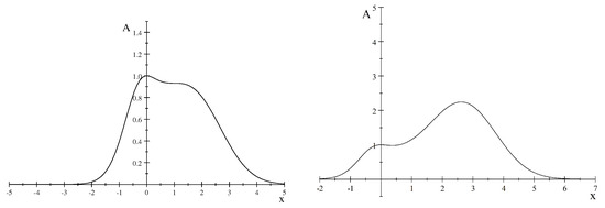
The corresponding fitness function is

$$A\left(x\right)=B\left(x\right)=\alpha exp\left({\displaystyle \frac{-\frac{x^2}{2}+px-parctanx}{{\sigma }^2}}\right),$$

(46)

where $\alpha >0$. Since $A\left(0\right)=\alpha$ and $A\left(1\right)=\alpha e^{{\displaystyle \frac{3-\pi }{2}}}<\alpha$ for $p=2$ and ${\sigma }^2=1$, we conclude that the zero equilibrium $E_0=0$ is ESS (evolutionary stable), since it is located at a global maximum of the fitness function, see [9,10,15]. On the other hand, if $p>2$ and ${\sigma }^2=1$, then $A\left(0\right)=\alpha$ and $A\left(E_{+}\right)>\alpha$, which means that the positive equilibrium point $E_{+}$ is ESS since it is located at the global maximum of the fitness function. See Figure 1.

Figure 1. The graphs of fitness function (46) for Equation (45) for ${\sigma }^2=1$, $\alpha =1$ and $p=2$ and $p=3$.

4. Conclusions

In this paper, we use several techniques to obtain some global attractivity results for non-autonomous cooperative systems of difference equations. The first technique we use is based on the difference inequalities theory which leads to some interesting results for the cooperative systems of any order when coefficients are asymptotically constants. Then, we used another technique specially designed for non-autonomous systems to obtain global attractivity results under weaker conditions on non-autonomous coefficients such as boundedness without convergence. Finally, we used a geometrical method to prove the global asymptotic stability of an autonomous system (25) which is a limiting equation for a non-autonomous cooperative system (34), and so we obtain the global attractivity of the equilibrium of (34). Our results have some analog results for two-dimensional competitive systems in [14], but unlike the results in [14] these results be extended to n-dimensional cooperative systems. Our results can not be derived from incorrect results in [13] without further verifications. The results in [13] need some extra conditions to be correct, in which case they might have the potential to be applicable to our examples. In the last section, we provide global dynamics of some cooperative evolutionary models, also known as Darwinian models, which leads to the problems of describing the global attractivity of non-autonomous cooperative systems of difference equations, see [9,10,11,12,15] for the basic results of this theory.

References

- Bilgin, A.; Kulenović, M.R.S. Global Attractivity for Nonautonomous Difference Equation via Linearization. J. Comput. Anal. Appl. 2017, 23, 1311–1322. [Google Scholar]
- Allen, L. An Introduction to Mathematical Biology; Parson: Boston, MA, USA, 2006; Available online: https://www.pearson.com/en-us/subject-catalog/p/introduction-to-mathematical-biology-an/P200000006070/9780130352163 (accessed on 15 September 2024).
- Bilgin, A.; Kulenović, M.R.S. Global Asymptotic Stabilty for Discrete Single Species Population Models. Discret. Nat. Soc. 2017, 2017, 5963594. [Google Scholar] [CrossRef]
- Cima, A.; Gasull, A.; Manosa, V. Asymptotic Stability for Block Triangular Maps. Sarajevo J. Math. 2022, 18, 25–44. Available online: https://upcommons.upc.edu/bitstream/handle/2117/375676/03-Anna_Cima-Armengol_Gasull-Victor20Manosa.pdf?sequence=3 (accessed on 15 September 2024). [CrossRef]
- Jamieson, W.; Merino, O. Asymptotic behavior results for solutions to some nonlinear difference equations. J. Math. Anal. Appl. 2015, 430, 614–632. [Google Scholar] [CrossRef]
- Krause, U. Positive Dynamical Systems in Discrete Time. Theory, Models, and Applications; De Gruyter Studies in Mathematics, 62; De Gruyter: Berlin, Germany, 2015. [Google Scholar] [CrossRef]
- Thieme, H.R. Mathematics in Population Biology; Princeton Series in Theoretical and Computational Biology; Princeton University Press: Princeton, NJ, USA, 2003; Available online: https://press.princeton.edu/books/paperback/9780691092911/mathematics-in-population-biology (accessed on 15 September 2024).
- Ackleh, A.S.; Cushing, J.M.; Salceanu, P.L. On the dynamics of evolutionary competition models. Nat. Resour. Model. 2015, 28, 380–397. Available online: https://onlinelibrary.wiley.com/doi/epdf/10.1111/nrm.12074 (accessed on 15 September 2024). [CrossRef]
- Cushing, J.M. An evolutionary Beverton–Holt model. In Theory and Applications of Difference Equations and Discrete Dynamical Systems; Springer: Heidelberg, Germany, 2014; pp. 127–141. [Google Scholar]
- Cushing, J.M. One Dimensional Maps as Population and Evolutionary Dynamic Models. In Applied Analysis in Biological and Physical Sciences; Springer: New Delhi, India, 2016; pp. 41–62. Available online: https://link.springer.com/chapter/10.1007/978-81-322-3640-5_3 (accessed on 15 September 2024).
- Cushing, J.M. Difference equations as models of evolutionary population dynamics. J. Biol. Dyn. 2019, 13, 103–127. [Google Scholar] [CrossRef] [PubMed]
- Cushing, J.M. A Darwinian Ricker Equation, Progres on Difference Equations and Discrete Dynamical Systems. In Proceedings of the 25th ICDEA, London, UK, 24–28 June 2019; pp. 231–243. [Google Scholar]
- Mokni, K.; Elaydi, S.; CH-Chaoui, M.; Eladdadi, A. Discrete evolutionary population models: A new approach. J. Biol. Dyn. 2020, 14, 454–478. [Google Scholar] [CrossRef] [PubMed]
- Kulenović, M.R.S.; Nurkanović, M.; Nurkanović, Z.; Trolle, S. Asymptotic Behavior of Certain Non-autonomous Planar Competitive Systems of Difference Equations. Mathematics 2023, 11, 3909. Available online: https://www.mdpi.com/2227-7390/11/18/3909# (accessed on 15 September 2024). [CrossRef]
- Vincent, T.L.; Brown, J.S. Evolutionary Game Theory, Natural, Selection, and Darwinian Dynamics; Cambridge University Press: Cambridge, NY, USA, 2005. [Google Scholar] [CrossRef]
- Fisher, R.A. The Genetical Theory of Natural Selection: A Complete Variorum Edition; Oxford University Press: Oxford, UK, 1930. [Google Scholar]
- Lande, R. A quantitative genetic theory of life history evolution. Ecology 1982, 33, 607–615. [Google Scholar] [CrossRef]
- Kulenović, M.R.S.; Merino, O. Discrete Dynamical Systems and Difference Equations with Mathematica; Chapman and Hall/CRC: Boca Raton, FL, USA; London, UK, 2002. [Google Scholar] [CrossRef]
- Elaydi, S. An Introduction to Difference Equations, 3rd ed.; Undergraduate Texts in Mathematics; Springer: New York, NY, USA, 2005. [Google Scholar]
- Elaydi, S. Discrete Chaos; Chapman& Hall/CRC Press: Boca Raton, FL, USA, 2000. [Google Scholar]
- Best, J.; Castillo-Chavez, C.; Yakubu, A. Hierarchical competition in discrete-time models with dispersal. Fields Inst. Commun. 2003, 36, 59–72. Available online: https://www.academia.edu/68711973/Hierarchical_competition_in_discrete_time_models_with_dispersal (accessed on 15 September 2024).
- Franke, J.E.; Yakubu, A.-A. Mutual exclusion versus coexistence for discrete competitive systems. J. Math. Biol. 1991, 30, 161–168. Available online: https://www.academia.edu/9570439/Mutual_exclusion_versus_coexistence_for_discrete_competitive_systems (accessed on 15 September 2024). [CrossRef]
- Franke, J.E.; Yakubu, A.-A. Global attractors in competitive systems. Nonlin. Anal. TMA 1991, 16, 111–129. [Google Scholar] [CrossRef]
- Franke, J.E.; Yakubu, A.-A. Geometry of exclusion principles in discrete systems. J. Math. Anal. Appl. 1992, 168, 385–400. Available online: https://core.ac.uk/download/pdf/82126078.pdf (accessed on 15 September 2024). [CrossRef]
- Kocic, V.; Ladas, G. Global Behavior of Nonlinear Difference Equations of Higher Order with Applications; Kluwer Academic Publishers: Dordrecht, The Netherlands, 1993. [Google Scholar]
- Lakshmikantham, V.; Trigiante, D. Theory of Difference Equations: Numerical Methods and Applications, 2nd ed.; Monographs and Textbooks in Pure and Applied Mathematics, 251; Marcel Dekker, Inc.: New York, NY, USA, 2002; p. x+300. [Google Scholar]
- Kulenović, M.R.S.; Nurkanović, M. Global Asympotic Behavior of a Two-dimensuional System of Difference Equations Modelling Cooperation. J. Differ. Equ. Appl. 2003, 9, 149–159. Available online: https://scholar.google.com/citations?view_op=view_citation&hl=hr&user=pqOYDPoAAAAJ&citation_for_view=pqOYDPoAAAAJ:eQOLeE2rZwMC (accessed on 15 September 2024). [CrossRef]
- Xueying, D.; Jianquan, L.; Xiangyong, C. Lyapunov-based stability of time-triggered impulsive logical dynamic networks. Nonlinear Anal. Hybrid Syst. 2024, 51, 101417. [Google Scholar]
- Yanmei, X.; Jinke, H.; Ziqiang, T.; Xiangyong, C. Stability analysis and design of cooperative control for linear delta operator system. AIMS Math. 2023, 8, 12671–12693. [Google Scholar]
- Kulenović, M.R.S.; Merino, M.O.; Nurkanović, M. Global dynamics of certain competitive system in the plane. J. Differ. Equ. Appl. 2012, 18, 1951–1966. Available online: https://scholar.google.com/citations?view_op=view_citation&hl=hr&user=pqOYDPoAAAAJ&cstart=20&pagesize=80&sortby=pubdate&citation_for_view=pqOYDPoAAAAJ:Se3iqnhoufwC (accessed on 15 September 2024). [CrossRef]
- Ch-Chaoui, M.; Mokni, K. A discrete evolutionary Beverton–Holt population model. Int. J. Dyn. Control 2023, 11, 1060–1075. Available online: https://link.springer.com/article/10.1007/s40435-022-01035-y (accessed on 15 September 2024). [CrossRef]
- Mokni, K.; Ch-Chaoui, M. Complex dynamics and bifurcation analysis for a Beverton–Holt population model with Allee effect. Int. J. Biomath. 2023, 16, 2250127. [Google Scholar] [CrossRef]
Disclaimer/Publisher’s Note: The statements, opinions and data contained in all publications are solely those of the individual author(s) and contributor(s) and not of MDPI and/or the editor(s). MDPI and/or the editor(s) disclaim responsibility for any injury to people or property resulting from any ideas, methods, instructions or products referred to in the content. |
© 2024 by the authors. Licensee MDPI, Basel, Switzerland. This article is an open access article distributed under the terms and conditions of the Creative Commons Attribution (CC BY) license (https://creativecommons.org/licenses/by/4.0/).