Elliptic Quaternion Matrices: Theory and Algorithms

Abstract

In this study, we obtained results for the computation of eigen-pairs, singular value decomposition, pseudoinverse, and the least squares problem for elliptic quaternion matrices. Moreover, we established algorithms based on these results and provided illustrative numerical experiments to substantiate the accuracy of our conclusions. In the experiments, it was observed that the p-value in the algebra of elliptic quaternions directly affects the performance of the problem under consideration. Selecting the optimal p-value for problem-solving and the elliptic behavior of many physical systems make this number system advantageous in applied sciences.

1. Introduction

Eigenvalues and eigenvectors, singular value decomposition, the pseudoinverse, and the least squares solution form the foundational pillars of matrix theory, with significant applications in diverse fields such as theoretical and computational mathematics, image and signal processing, principal component analysis, data compression, machine learning, deep learning, etc. For example, Israel and Greville comprehensively treated eigenvalues, eigenvectors, singular value decomposition, the pseudoinverse, and the least squares solution. The book explores the interconnections between these concepts, presenting both their underlying theories and practical applications across various fields [1]. Samar et al. presented a K-weighted pseudoinverse and gave results for condition numbers for the solution of the least squares problem with equality constraint [2]. Samar et al. explored the conditioning theory of the $\mathcal{M}\mathcal{L}$-weighted least squares and $\mathcal{M}\mathcal{L}$-weighted pseudoinverse problems [3]. Simsek focused on obtaining least-squares solutions for generalized Sylvester-type quaternion matrix equations using pseudoinverses and applied these solutions to color image restoration processes [4]. Dian et al. presented a novel hyperspectral image and multispectral image fusion method based on the subspace representation and convolutional neural network denoiser. They obtained the subspaces via singular value decomposition of a high-resolution hyperspectral image [5]. Hashemipour et al. proposed a new lossy data compression framework centered on optimal singular value decomposition for big data compression [6]. Wang and Zhu focused on the implementation of data reduction algorithms in machine learning by using eigenvalues-eigenvectors, singular value decomposition, and principal component analysis [7].

These mathematical concepts not only form the basis of numerous applications but also extend to n-dimensional hypercomplex number systems. There is a generalization involving 2-dimensional hypercomplex numbers [8]. The following is the definition of these numbers, known as generalized complex numbers:

$$q_{\left(g\right)}=q_{\left(g\right),r}+q_{\left(g\right),i}i,$$

where $q_{\left(g\right),r},q_{\left(g\right),i}\in \mathbb{R},i\notin \mathbb{R}$ and $i^2=p\left(p\in \mathbb{R}\right).$ Generalized Segre quaternions are generalized complex numbers extended to 4 dimensions. Generalized Segre quaternions are defined as follows:

$$q_{\left(GS\right)}=q_{\left(GS\right),r}+q_{\left(GS\right),i}i+q_{\left(GS\right),j}j+q_{\left(GS\right),k}k,$$

where $q_{\left(GS\right),r},q_{\left(GS\right),i},q_{\left(GS\right),j},q_{\left(GS\right),k}\in \mathbb{R},i,j,k\notin \mathbb{R}$. The multiplication rules for units $i,j$ and k are given below:

$$i^2=k^2=p,j^2=1,ij=ji=k,jk=kj=i,ki=ik=pj,p\in \mathbb{R}.$$

Based on the value of p, generalized complex numbers and Segre quaternions are classified into three categories: they are referred to as hyperbolic complex numbers and hyperbolic quaternions when $p>0$, parabolic complex numbers and parabolic quaternions when $p=0$, and elliptic complex numbers and elliptic quaternions when $p<0$, [8,9]. Each number system has various scientific and technological applications. For example, some problemsin non-Euclidean geometries can be solved by hyperbolic complex numbers and hyperbolic quaternions [10]. In domains like robotic control and spatial mechanics, parabolic complex (dual) numbers and parabolic quaternions are employed [11]. On the other hand, as numerous physical systems demonstrate elliptical behavior, the practical applications of elliptic complex numbers and elliptic quaternions in applied science are noteworthy. One of the examples is that, Ozdemir defined elliptic quaternions (non-commutative) and generated an elliptical rotation matrix for the motion of a point on an ellipse through some angle about a vector using those quaternions [12]. Dundar et al. studied elliptical harmonic motion, which is the superposition of two simple harmonic motions in perpendicular directions with the same angular frequency and phase difference of ${\displaystyle \frac{\pi }{2}}$ using elliptic complex numbers [13]. Derin and Gungor proposed the generalization of gravity, including the Proca-type and gravitomagnetic monopole by means of elliptic biquaternions [14]. Catoni et al. introduced algebraic properties and the differential conditions of elliptic quaternionic systems [9]. Additionally, Catoni et al. studied the constant curvature spaces associated with the geometry generated by elliptic quaternions. They formulated geodesic equations within the context of Riemann geometry [15]. Gua et al. defined the elliptic quaternionic canonical transform and investigated Parseval’s theorem with the help of this transform [16]. Yuan et al. obtained the Hermitian solutions of the elliptic quaternion matrix equation $\left(AXB,CXD\right)=\left(E,G\right)$ [17]. Tosun and Kosal characterized the existence of the solution to Sylvester s-conjugate elliptic quaternion matrix equations. They obtained the solution explicitly using a real representation of an elliptic quaternion matrix [18]. Gai and Huang developed a new convolutional neural network with elliptic quaternion values. They conducted extensive experiments on colour image classification and colour image denoising to evaluate the performance of the proposed convolutional neural network [19]. Guo et al. studied the problem of solutions to Maxwell’s equations of elliptic quaternions using a real representation of elliptic quaternion matrices [20]. Atali et al. obtained the elliptic quaternionic least-squares solution with the minimum norm of the elliptic quaternion matrix equation $AX=B$. Furthermore, leveraging the insights derived from their theories, they developed a novel color image restoration model known as the elliptical quaternionic least squares restoration filter [21].

As observed, the elliptic quaternions and their matrices find numerous practical applications in various branches of applied sciences. Thus, further study of the theoretical properties and numerical computations of elliptic quaternions and their matrices is becoming increasingly necessary. In this regard, we derive outcomes concerning the computation of eigen-pairs, singular value decomposition, pseudoinverse, and least squares solutions with the minimum norm for elliptic quaternion matrices. Additionally, algorithms are formulated based on these results, accompanied by illustrative numerical experiments to validate our findings’ precision empirically. Within the context of this paper, the following notations are employed. Let $\mathbb{R}$, $\mathbb{C}$, ${\mathbb{C}}_p$, and ${\mathbb{H}}_p$ denote the sets of real numbers, complex numbers, elliptic complex numbers, and elliptic quaternions, respectively. ${\mathbb{R}}^{m\times n}$, ${\mathbb{C}}^{m\times n}$, ${\mathbb{C}}_p^{m\times n}$, and ${\mathbb{H}}_p^{m\times n}$ denote the set of all $m\times n$ matrices on $\mathbb{R}$, $\mathbb{C}$, ${\mathbb{C}}_p$ and ${\mathbb{H}}_p$, respectively. Throughout the study, we will also denote elliptic complex numbers as EC numbers and elliptic quaternions as EQs for short. Also, we use the following notations: $q_{\left(\square \right)}$ represents a complex number when $\square =c$, an EC number when $\square =e$, and an EQ when $\square =E$. Similarly, $Q_{\left(\square \right)}$ denotes a complex matrix when $\square =c$, an EC matrix when $\square =e$, and an EQ matrix when $\square =E$.

2. Preliminaries

In this section, some basic algebraic properties and notations for EC numbers and EQs are given. This section provides the basis for further operations, which are discussedin the following sections.

An EC number $q_{\left(e\right)}$ is denoted by $q_{\left(e\right)}=q_{\left(e\right),r}+q_{\left(e\right),i}i$, where $i^2=p<0$ and $q_{\left(e\right),r},q_{\left(e\right),i},p\in \mathbb{R}$. The real and imaginary parts of $q_{\left(e\right)}$ are denoted by $Re\left(q_{\left(e\right)}\right)=q_{\left(e\right),r}$ and $Im\left(q_{\left(e\right)}\right)=q_{\left(e\right),i}$, respectively. The conjugate and norm of $q_{\left(e\right)}\in {\mathbb{C}}_p$ are defined as $\overline{q_{\left(e\right)}}=q_{\left(e\right),r}-q_{\left(e\right),i}i\mathrm{and}{∥q_{\left(e\right)}∥}_p=\sqrt{q_{\left(e\right),r}^2-p{q}_{\left(e\right),i}^2},$ respectively [22]. The multiplication of two EC numbers $q_{1,\left(e\right)}=q_{1,\left(e\right),r}+q_{1,\left(e\right),i}i$ and $q_{2,\left(e\right)}=q_{2,\left(e\right),r}+q_{2,\left(e\right),i}i$ is defined as

$$q_{1,\left(e\right)}{q}_{2,\left(e\right)}=\left(q_{1,\left(e\right),r}{q}_{2,\left(e\right),r}+p{q}_{1,\left(e\right),i}{q}_{2,\left(e\right),i}\right)+i\left(q_{1,\left(e\right),r}{q}_{2,\left(e\right),i}+q_{2,\left(e\right),r}{q}_{1,\left(e\right),i}\right).$$

An EC matrix $Q_{\left(e\right)}$ is denoted as $Q_{\left(e\right)}=Q_{\left(e\right),r}+Q_{\left(e\right),i}i$, where $i^2=p<0$, $p\in \mathbb{R}$, and $Q_{\left(e\right),r}$, $Q_{\left(e\right),i}\in {\mathbb{R}}^{m\times n}$. The conjugate, transpose, conjugate transpose and Frobenius norm of $Q_{\left(e\right)}\in {\mathbb{C}}_p^{m\times n}$ are defined by $\overline{Q_{\left(e\right)}}=Q_{\left(e\right),r}-Q_{\left(e\right),i}i$, $Q_{\left(e\right)}^T=Q_{\left(e\right),r}^T+Q_{\left(e\right),i}^{T}i,Q_{\left(e\right)}^{\ast }=Q_{\left(e\right),r}^T-Q_{\left(e\right),i}^{T}i,$ and $\parallel Q_{\left(e\right)}{\parallel }_p=\sqrt{\parallel Q_{\left(e\right),r}{\parallel }^2-p{\parallel Q_{\left(e\right),i}\parallel }^2}$, respectively. The multiplication of two EC matrices $Q_{1,\left(e\right)}=Q_{1,\left(e\right),r}+Q_{1,\left(e\right),i}i$ and $Q_{2,\left(e\right)}=Q_{2,\left(e\right),r}+Q_{2,\left(e\right),i}i$ is defined as

$$Q_{1,\left(e\right)}{Q}_{2,\left(e\right)}=\left(Q_{1,\left(e\right),r}{Q}_{2,\left(e\right),r}+p{Q}_{1,\left(e\right),i}{Q}_{2,\left(e\right),i}\right)+i\left(Q_{1,\left(e\right),r}{Q}_{2,\left(e\right),i}+Q_{2,\left(e\right),r}{Q}_{1,\left(e\right),i}\right).$$

There exists an isomorphism between EC matrices and complex matrices, as depicted in the following:

$$\begin{array}{c}{\mathrm{H}}_p:{\mathbb{C}}_p^{m\times n}\to {\mathbb{C}}^{m\times n}\hfill \\ Q_{\left(e\right)}=Q_{\left(e\right),r}+Q_{\left(e\right),i}i\to {\mathrm{H}}_p\left(Q_{\left(e\right)}\right)=Q_{\left(c\right)}=Q_{\left(e\right),r}+I\sqrt{-p}{Q}_{\left(e\right),i},\hfill \end{array}$$

where I represents the complex unit ($I^2=-1$). Some algebraic operations of this isomorphism are listed below, where $Q_{\left(e\right),1}$ and $Q_{\left(e\right),2}$ are EC matrices of appropriate sizes:

(a)

$H_p\left(Q_{\left(e\right),1}{Q}_{\left(e\right),2}\right)=H_p\left(Q_{\left(e\right),1}\right)H_p\left(Q_{\left(e\right),2}\right)$,

(b)

${\left(H_p\left(Q_{\left(e\right),1}\right)\right)}^T=H_p\left(Q_{\left(e\right),1}^T\right)$,

(c)

${\left(H_p\left(Q_{\left(e\right),1}\right)\right)}^{\ast }=H_p\left(Q_{\left(e\right),1}^{\ast }\right)$,

(d)

$\overline{\left(H_p\left(Q_{\left(e\right),1}\right)\right)}=H_p\left(\overline{Q_{\left(e\right),1}}\right)$.

Many algebraic properties of EC numbers (or matrices) can be derived from their corresponding complex counterparts using this isomorphism [8,23].

An EQ $q_{\left(E\right)}$ is denoted as $q_{\left(E\right)}=q_{\left(E\right),r}+q_{\left(E\right),i}i+q_{\left(E\right),j}j+q_{\left(E\right),k}k$, where $i^2=k^2=p<0$, $j^2=1$, $ij=ji=k$, $jk=kj=i$, $ki=ik=pj$, and $q_{\left(E\right),r},q_{\left(E\right),i},q_{\left(E\right),j},q_{\left(E\right),k},p\in \mathbb{R}$ [9,22]. An EQ $q_{\left(E\right)}$ is denoted in the forms:

$$q_{\left(E\right)}=\left(q_{\left(E\right),r}+i{q}_{\left(E\right),i}\right)+\left(q_{\left(E\right),j}+i{q}_{\left(E\right),k}\right)j=q_{\left(e\right),1}{e}_1+q_{\left(e\right),2}{e}_2,$$

where

$$q_{\left(e\right),1}=\left(q_{\left(E\right),r}+q_{\left(E\right),j}\right)+\left(q_{\left(E\right),i}+q_{\left(E\right),k}\right)i$$

and

$$q_{\left(e\right),2}=\left(q_{\left(E\right),r}-q_{\left(E\right),j}\right)+\left(q_{\left(E\right),i}-q_{\left(E\right),k}\right)i,$$

are EC numbers and $e_1={\displaystyle \frac{1+j}{2}},e_2={\displaystyle \frac{1-j}{2}}.$ Clearly, $e_1{e}_2=0,e_1+e_2=1$, $e_1^2=e_1$ and $e_2^2=e_2.$ As a result, $e_1$ and $e_2$ are disjoint idempotent units. The multiplication of two EQs $q_{1,\left(E\right)}=q_{1,\left(e\right),1}{e}_1+q_{1,\left(e\right),2}{e}_2$ and $q_{2,\left(E\right)}=q_{2,\left(e\right),1}{e}_1+q_{2,\left(e\right),2}{e}_2$ is defined by

$$\begin{array}{c}{q}_{1,\left(E\right)}{q}_{2,\left(E\right)}=\left(q_{1,\left(e\right),1}{q}_{2,\left(e\right),1}\right)e_1+\left(q_{1,\left(e\right),2}{q}_{2,\left(e\right),2}\right)e_2.\hfill \end{array}$$

The conjugate and norm of the EQ $q_{\left(E\right)}=q_{\left(e\right),1}{e}_1+q_{\left(e\right),2}{e}_2$ are defined by $\overline{q_{\left(E\right)}}=\overline{q_{\left(e\right),1}}{e}_1+\overline{q_{\left(e\right),2}}{e}_2$ and ${∥q_{\left(E\right)}∥}_p={\displaystyle \frac{1}{\sqrt{2}}}\sqrt{\left({∥q_{\left(e\right),1}∥}_p^2+{∥q_{\left(e\right),2}∥}_p^2\right)},$ respectively.

An EQ matrix $Q_{\left(E\right)}$ is represented as

$$\begin{array}{c}{Q}_{\left(E\right)}=Q_{\left(E\right),r}+Q_{\left(E\right),i}i+Q_{\left(E\right),j}j+Q_{\left(E\right),k}k=\left(Q_{\left(E\right),r}+Q_{\left(E\right),i}i\right)+j\left(Q_{\left(E\right),j}+Q_{\left(E\right),k}i\right)\\ =Q_{\left(e\right),1}{e}_1+Q_{\left(e\right),2}{e}_2,\end{array}$$

(1)

where

$$Q_{\left(e\right),1}=\left(Q_{\left(E\right),r}+Q_{\left(E\right),j}\right)+\left(Q_{\left(E\right),i}+Q_{\left(E\right),k}\right)i$$

and

$$Q_{\left(e\right),2}=\left(Q_{\left(E\right),r}-Q_{\left(E\right),j}\right)+\left(Q_{\left(E\right),i}-Q_{\left(E\right),k}\right)i$$

are EC matrices and $Q_{\left(E\right),r},Q_{\left(E\right),i},Q_{\left(E\right),j},Q_{\left(E\right),k}\in {\mathbb{R}}^{m\times n}$ [18,21]. The multiplication of two EQ matrices $Q_{1,\left(E\right)}=Q_{1,\left(e\right),1}{e}_1+Q_{1,\left(e\right),2}{e}_2$ and $Q_{2,\left(E\right)}=Q_{2,\left(e\right),1}{e}_1+Q_{2,\left(e\right),2}{e}_2$ is defined by

$$\begin{array}{c}{Q}_{1,\left(E\right)}{Q}_{2,\left(E\right)}=\left(Q_{1,\left(e\right),1}{Q}_{2,\left(e\right),1}\right)e_1+\left(Q_{1,\left(e\right),2}{Q}_{2,\left(e\right),2}\right)e_2.\hfill \end{array}$$

The conjugate, transpose, conjugate transpose, and Frobenius norm of EQ matrix $Q_{\left(E\right)}=Q_{\left(e\right),1}{e}_1+Q_{\left(e\right),2}{e}_2\in {\mathbb{H}}_p^{m\times n}$ are defined by $\overline{Q_{\left(E\right)}}=\overline{Q_{\left(e\right),1}}{e}_1+\overline{Q_{\left(e\right),2}}{e}_2$, $Q_{\left(E\right)}^T=Q_{\left(e\right),1}^T{e}_1+Q_{\left(e\right),2}^T{e}_2$, $Q_{\left(E\right)}^{\ast }=\overline{Q_{\left(e\right),1}^T}{e}_1+\overline{Q_{\left(e\right),2}^T}{e}_2$ and $\begin{array}{c}{∥Q_{\left(E\right)}∥}_p={\displaystyle \frac{1}{\sqrt{2}}}\sqrt{\left({∥Q_{\left(e\right),1}∥}_p^2+{∥Q_{\left(e\right),2}∥}_p^2\right)}.\hfill \end{array}$

3. Eigenvalues and Eigenvectors, Singular Value Decomposition, Pseudoinverse, and Least Squares Problem for EQ Matrices

In the ensuing discourse, we delineate a series of lemmas pivotal for the computation of eigen-pairs, singular value decomposition, pseudoinverse, and the resolution of the least squares problem specifically tailored for EC matrices. Subsequently, leveraging these foundational lemmas, we derive the pertinent theoretical framework associated with elliptic quaternion matrices.

3.1. EC Matrices

Lemma 1.

A polynomial function of degree N with EC number coefficients presented by

$$f_p\left(x_{\left(e\right)}\right)=x_{\left(e\right)}^N+q_{\left(e\right),N-1}{x}_{\left(e\right)}^{N-1}+\dots +q_{\left(e\right),1}{x}_{\left(e\right)}+q_{\left(e\right),0}$$

has exactly N zeros in the set of EC numbers.

Proof. 

Let

$$f_p\left(x_{\left(e\right)}\right)=x_{\left(e\right)}^N+q_{\left(e\right),N-1}{x}_{\left(e\right)}^{N-1}+\dots +q_{\left(e\right),1}{x}_{\left(e\right)}+q_{\left(e\right),0}$$

be a polynomial of degree N with EC coefficients and values. Its complex representation is as follows:

$${\mathrm{H}}_p\left(f_p\left(x_{\left(e\right)}\right)\right)={\mathrm{H}}_p{\left(x_{\left(e\right)}\right)}^N+{\mathrm{H}}_p\left(q_{\left(e\right),N-1}\right){\mathrm{H}}_p{\left(x_{\left(e\right)}\right)}^{N-1}+\dots +{\mathrm{H}}_p\left(q_{\left(e\right),1}\right){\mathrm{H}}_p\left(x_{\left(e\right)}\right)+{\mathrm{H}}_p\left(q_{\left(e\right),0}\right).$$

Since this representation is a polynomial of degree N with complex coefficients and values, the fundamental theorem of algebra tells us that it has exactly N roots. Suppose that the complex number $x_{\left(c\right)}=x_{\left(c\right),r}+x_{\left(c\right),i}I$ is a root of the polynomial ${\mathrm{H}}_p\left(f_p\left(x_{\left(e\right)}\right)\right)$. Then, we have:

$${\mathrm{H}}_p\left(f_p\left(x_{\left(e\right)}\right)\right)={\left(x_{\left(c\right)}\right)}^N+{\mathrm{H}}_p\left(q_{\left(e\right),N-1}\right){\left(x_{\left(c\right)}\right)}^{N-1}+\dots +{\mathrm{H}}_p\left(q_{\left(e\right),1}\right)\left(x_{\left(c\right)}\right)+{\mathrm{H}}_p\left(q_{\left(e\right),0}\right)=0.$$

Applying the inverse of the isomorphism ${\mathrm{H}}_p$ to both sides of the above equation, we get:

$$f_p\left(x_{\left(e\right)}\right)={\mathrm{H}}_{\mathrm{p}}^{-1}{\left({\mathrm{x}}_{\left(\mathrm{c}\right)}\right)}^{\mathrm{N}}+{\mathrm{q}}_{\left(\mathrm{e}\right),\mathrm{N}-1}{\mathrm{H}}_{\mathrm{p}}^{-1}{\left({\mathrm{x}}_{\left(\mathrm{c}\right)}\right)}^{\mathrm{N}-1}+\dots +{\mathrm{q}}_{\left(\mathrm{e}\right),1}{\mathrm{H}}_{\mathrm{p}}^{-1}\left({\mathrm{x}}_{\left(\mathrm{c}\right)}\right)+{\mathrm{q}}_{\left(\mathrm{e}\right),0}.$$

This simplifies to:

$$f_p\left(x_{\left(e\right)}\right)={\left(x_{\left(c\right),r}+{\displaystyle \frac{i}{\sqrt{-p}}}{x}_{\left(c\right),i}\right)}^N+q_{\left(e\right),N-1}{\left(x_{\left(c\right),r}+{\displaystyle \frac{i}{\sqrt{-p}}}{x}_{\left(c\right),i}\right)}^{N-1}+\dots +q_{\left(e\right),1}\left(x_{\left(c\right),r}+{\displaystyle \frac{i}{\sqrt{-p}}}{x}_{\left(c\right),i}\right)+q_{\left(e\right),0}=0.$$

Therefore, if $x_{\left(c\right)}=x_{\left(c\right),r}+x_{\left(c\right),i}I$ is a root of the polynomial ${\mathrm{H}}_p\left(f_p\left(x_{\left(e\right)}\right)\right)$, then the EC number $x_{\left(e\right)}=x_{\left(c\right),r}+{\displaystyle \frac{i}{\sqrt{-p}}}{x}_{\left(c\right),i}$ is a root of the polynomial $f_p\left(x_{\left(e\right)}\right)$. As a result, $f_p\left(x_{\left(e\right)}\right)$ has exactly N roots.    □

Lemma 2.

An EC matrix $Q_{\left(e\right)}\in {\mathbb{C}}_p^{n\times n}$ has at most n elliptic eigenvalues.

Proof. 

Since the characteristic polynomial $f_p\left({\lambda }_{\left(e\right)}\right)=det(Q_{\left(e\right)}-{\lambda }_{\left(e\right)}{I}_n)$ of the matrix $Q_{\left(e\right)}\in {\mathbb{C}}_p^{n\times n}$ is an n-th order polynomial with EC coefficients and values, by Lemma 1, the EC matrix $Q_{\left(e\right)}$ has at most n eigenvalues.    □

Lemma 3.

Let the eigenvalues of an complex matrix ${\mathrm{H}}_p\left(Q_{\left(e\right)}\right)$ be denoted by ${\lambda }_{{\mathrm{H}}_p\left(Q_{\left(e\right)}\right)}$, and let the corresponding eigenvectors be represented by $x_{{\mathrm{H}}_p\left(Q_{\left(e\right)}\right)}.$ Then, the eigenvalues of the EC matrix $Q_{\left(e\right)}\in {\mathbb{C}}_p^{n\times n}$ are given by

$${\lambda }_{\left(e\right)}=Re({\lambda }_{{\mathrm{H}}_p\left(Q_{\left(e\right)}\right)})+{\displaystyle \frac{i}{\sqrt{-p}}}Im({\lambda }_{{\mathrm{H}}_p\left(Q_{\left(e\right)}\right)})$$

and the corresponding eigenvectors are given by

$$x_{\left(e\right)}=Re(x_{{\mathrm{H}}_p\left(Q_{\left(e\right)}\right)})+{\displaystyle \frac{i}{\sqrt{-p}}}Im(x_{{\mathrm{H}}_p\left(Q_{\left(e\right)}\right)}).$$

The converse of this lemma is also true.

Proof. 

Let $Q_{\left(e\right)}\in {\mathbb{C}}_p^{n\times n}$ be an EC matrix, and the eigenvalues of an complex matrix ${\mathrm{H}}_p\left(Q_{\left(e\right)}\right)$ be denoted by ${\lambda }_{{\mathrm{H}}_p\left(Q_{\left(e\right)}\right)}$, and let the corresponding eigenvectors be represented by $x_{{\mathrm{H}}_p\left(Q_{\left(e\right)}\right)}.$ Then, we have ${\mathrm{H}}_p\left(Q_{\left(e\right)}\right)x_{{\mathrm{H}}_p\left(Q_{\left(e\right)}\right)}={\lambda }_{{\mathrm{H}}_p\left(Q_{\left(e\right)}\right)}{x}_{{\mathrm{H}}_p\left(Q_{\left(e\right)}\right)}.$ Applying the inverse of the isomorphism ${\mathrm{H}}_p$ to both sides of the last equation, we get:

$$Q_{\left(e\right)}{\mathrm{H}}_p^{-1}\left(x_{{\mathrm{H}}_p\left(Q_{\left(e\right)}\right)}\right)={\mathrm{H}}_p^{-1}\left({\lambda }_{{\mathrm{H}}_p\left(Q_{\left(e\right)}\right)}\right){\mathrm{H}}_p^{-1}\left(x_{{\mathrm{H}}_p\left(Q_{\left(e\right)}\right)}\right).$$

Thus, we get

$${\lambda }_{\left(e\right)}=Re\left({\lambda }_{{\mathrm{H}}_p\left(Q_{\left(e\right)}\right)}\right)+{\displaystyle \frac{i}{\sqrt{-p}}}Im\left({\lambda }_{{\mathrm{H}}_p\left(Q_{\left(e\right)}\right)}\right),$$

and

$$x_{\left(e\right)}=Re\left(x_{{\mathrm{H}}_p\left(Q_{\left(e\right)}\right)}\right)+{\displaystyle \frac{i}{\sqrt{-p}}}Im\left(x_{{\mathrm{H}}_p\left(Q_{\left(e\right)}\right)}\right).$$

□

Lemma 4.

Let $Q_{\left(e\right)}\in {\mathbb{C}}_p^{n\times n}$. An EC matrix $Q_{\left(e\right)}$ is nonsingular if and only if the complex matrix ${\mathrm{H}}_p\left(Q_{\left(e\right)}\right)$ is nonsingular. If ${\mathrm{H}}_p\left(Q_{\left(e\right)}\right)$ is nonsingular, then

$$Q_{\left(e\right)}^{-1}=Re\left({\left({\mathrm{H}}_p\left(Q_{\left(e\right)}\right)\right)}^{-1}\right)+{\displaystyle \frac{i}{\sqrt{-p}}}Im\left({\left({\mathrm{H}}_p\left(Q_{\left(e\right)}\right)\right)}^{-1}\right).$$

Proof. 

Let the EC matrix ${\mathrm{Q}}_{\left(e\right)}={\mathrm{Q}}_{\left(e\right),r}+{\mathrm{Q}}_{\left(e\right),i}i$ be nonsingular. Then, there exists an inverse matrix ${\mathrm{Q}}_{\left(e\right)}^{-1}\in {\mathbb{C}}_p^{n\times n}$ such that ${\mathrm{Q}}_{\left(e\right)}{\mathrm{Q}}_{\left(e\right)}^{-1}={\mathrm{Q}}_{\left(e\right)}^{-1}{\mathrm{Q}}_{\left(e\right)}=I_n.$ If we apply the isomorphism ${\mathrm{H}}_{\mathrm{p}}$ to both sides of the last equation, we obtain:

$${\mathrm{H}}_p\left({\mathrm{Q}}_{\left(e\right)}\right){\mathrm{H}}_p\left({\mathrm{Q}}_{\left(e\right)}^{-1}\right)={\mathrm{H}}_p\left({\mathrm{Q}}_{\left(e\right)}^{-1}\right){\mathrm{H}}_p\left({\mathrm{Q}}_{\left(e\right)}\right)=I_n.$$

Hence, we conclude that ${\left({\mathrm{H}}_p\left({\mathrm{Q}}_{\left(e\right)}\right)\right)}^{-1}={\mathrm{H}}_p\left({\mathrm{Q}}_{\left(e\right)}^{-1}\right).$ On the other hand, since

$${\mathrm{H}}_p\left({\mathrm{Q}}_{\left(e\right)}^{-1}\right)=Re\left({\left({\mathrm{H}}_p\left({\mathrm{Q}}_{\left(e\right)}\right)\right)}^{-1}\right)+IIm\left({\left({\mathrm{H}}_p\left({\mathrm{Q}}_{\left(e\right)}\right)\right)}^{-1}\right),$$

we can apply the inverse of the isomorphism ${\mathrm{H}}_p$ to this equation, yielding:

$${\mathrm{Q}}_{\left(e\right)}^{-1}=Re\left({\left({\mathrm{H}}_p\left({\mathrm{Q}}_{\left(e\right)}\right)\right)}^{-1}\right)+{\displaystyle \frac{i}{\sqrt{-p}}}Im\left({\left({\mathrm{H}}_p\left({\mathrm{Q}}_{\left(e\right)}\right)\right)}^{-1}\right).$$

□

Lemma 5.

Let $Q_{\left(e\right)}\in {\mathbb{C}}_p^{m\times n}$ be an EC matrix. The pseudoinverse of $Q_{\left(e\right)}$, denoted by ${\left(Q_{\left(e\right)}\right)}^{†}$, is given by

$${\left(Q_{\left(e\right)}\right)}^{†}=\mathrm{Re}\left({\left({\mathrm{H}}_{\mathrm{p}}\left(Q_{\left(e\right)}\right)\right)}^{†}\right)+{\displaystyle \frac{i}{\sqrt{-p}}}\mathrm{Im}\left({\left({\mathrm{H}}_{\mathrm{p}}\left(Q_{\left(e\right)}\right)\right)}^{†}\right),$$

where ${\left({\mathrm{H}}_{\mathrm{p}}\left(Q_{\left(e\right)}\right)\right)}^{†}$ is the pseudoinverse of the complex matrix ${\mathrm{H}}_{\mathrm{p}}\left({\mathrm{Q}}_{\left(\mathrm{e}\right)}\right)$.

Proof. 

Suppose that $Q_{\left(e\right)}^{†}$ is the pseudoinverse of the matrix $Q_{\left(e\right)}$. In that case, the following equations hold:

$$Q_{\left(e\right)}{Q}_{\left(e\right)}^{†}{Q}_{\left(e\right)}=Q_{\left(e\right)},Q_{\left(e\right)}^{†}{Q}_{\left(e\right)}{Q}_{\left(e\right)}^{†}=Q_{\left(e\right)}^{†},$$

$${\left(Q_{\left(e\right)}{Q}_{\left(e\right)}^{†}\right)}^{\ast }=Q_{\left(e\right)}{Q}_{\left(e\right)}^{†},{\left(Q_{\left(e\right)}^{†}{Q}_{\left(e\right)}\right)}^{\ast }=Q_{\left(e\right)}^{†}{Q}_{\left(e\right)}.$$

Applying the isomorphism ${\mathrm{H}}_p$ to the above equations, we get the following results:

$$\begin{array}{c}{\mathrm{H}}_p\left(Q_{\left(e\right)}\right){\mathrm{H}}_p\left(Q_{\left(e\right)}^{†}\right){\mathrm{H}}_p\left(Q_{\left(e\right)}\right)={\mathrm{H}}_p\left(Q_{\left(e\right)}\right),\hfill \\ {\mathrm{H}}_p\left(Q_{\left(e\right)}^{†}\right){\mathrm{H}}_p\left(Q_{\left(e\right)}\right){\mathrm{H}}_p\left(Q_{\left(e\right)}^{†}\right)={\mathrm{H}}_p\left(Q_{\left(e\right)}^{†}\right),\hfill \\ {\left({\mathrm{H}}_p\left(Q_{\left(e\right)}\right){\mathrm{H}}_p\left(Q_{\left(e\right)}^{†}\right)\right)}^{\ast }={\mathrm{H}}_p\left(Q_{\left(e\right)}\right){\mathrm{H}}_p\left(Q_{\left(e\right)}^{†}\right),\hfill \\ {\left({\mathrm{H}}_p\left(Q_{\left(e\right)}^{†}\right){\mathrm{H}}_p\left(Q_{\left(e\right)}\right)\right)}^{\ast }={\mathrm{H}}_p\left(Q_{\left(e\right)}^{†}\right){\mathrm{H}}_p\left(Q_{\left(e\right)}\right).\hfill \end{array}$$

As a result, we obtain the following pseudoinverse transformation under the isomorphism ${\mathrm{H}}_p$:

$${\left({\mathrm{H}}_p\left(Q_{\left(e\right)}\right)\right)}^{†}={\mathrm{H}}_p\left(Q_{\left(e\right)}^{†}\right),$$

and

$${\left(Q_{\left(e\right)}\right)}^{†}=Re\left({\left({\mathrm{H}}_p\left(Q_{\left(e\right)}\right)\right)}^{†}\right)+{\displaystyle \frac{i}{\sqrt{-p}}}Im\left({\left({\mathrm{H}}_p\left(Q_{\left(e\right)}\right)\right)}^{†}\right).$$

□

Lemma 6.

Let $Q_{\left(e\right)}\in {\mathbb{C}}_p^{m\times n}$. Suppose that the singular value decomposition of the complex matrix ${\mathrm{H}}_p\left(Q_{\left(e\right)}\right)$ is given by ${\mathrm{H}}_{\mathrm{p}}\left(Q_{\left(e\right)}\right)=U_{\left(c\right)}\Sigma V_{\left(c\right)}^{\ast }.$ Then, the singular value decomposition of the EC matrix $Q_{\left(e\right)}$ is

$$Q_{\left(e\right)}=U_{\left(e\right)}\Sigma V_{\left(e\right)}^{\ast },$$

where

$$U_{\left(e\right)}=\left(Re\left(U_{\left(c\right)}\right)+{\displaystyle \frac{i}{\sqrt{-p}}}Im\left(U_{\left(c\right)}\right)\right)and{V}_{\left(e\right)}=\left(Re\left(U_{\left(c\right)}\right)+{\displaystyle \frac{i}{\sqrt{-p}}}Im\left(U_{\left(c\right)}\right)\right).$$

The converse of this statement is also true.

Proof. 

Suppose that the singular value decomposition of the complex representation ${\mathrm{H}}_{\mathrm{p}}\left(Q_{\left(e\right)}\right)$ is given by:

$${\mathrm{H}}_{\mathrm{p}}\left(Q_{\left(e\right)}\right)=U_{\left(c\right)}\Sigma V_{\left(c\right)}^{\ast }.$$

Now, using the expansion of the real and imaginary parts of the unitary matrices, we have:

$${\mathrm{H}}_{\mathrm{p}}\left(Q_{\left(e\right)}\right)=\left(Re\left(U_{\left(c\right)}\right)+iIm\left(U_{\left(c\right)}\right)\right)\Sigma \left(Re\left(V_{\left(c\right)}^{\ast }\right)+iIm\left(V_{\left(c\right)}^{\ast }\right)\right).$$

Applying the inverse of the isomorphism ${\mathrm{H}}_{\mathrm{p}}$ to both sides of the last equation, we obtain:

$$Q_{\left(e\right)}=\left(Re\left(U_{\left(c\right)}\right)+{\displaystyle \frac{i}{\sqrt{-p}}}Im\left(U_{\left(c\right)}\right)\right)\Sigma \left(Re\left(V_{\left(c\right)}^{\ast }\right)+{\displaystyle \frac{i}{\sqrt{-p}}}Im\left(V_{\left(c\right)}^{\ast }\right)\right).$$

On the other hand, since $U_{\left(c\right)}$ and $V_{\left(c\right)}$ are unitary matrices, we have

$$\begin{array}{c}{U}_{\left(e\right)}{U}_{\left(e\right)}^{\ast }=\left(Re\left(U_{\left(c\right)}\right)+{\displaystyle \frac{i}{\sqrt{-p}}}Im\left(U_{\left(c\right)}\right)\right)\left(Re\left(U_{\left(c\right)}^T\right)-{\displaystyle \frac{i}{\sqrt{-p}}}Im\left(U_{\left(c\right)}^T\right)\right)\hfill \\ =I_n\hfill \end{array}$$

and

$$\begin{array}{c}{V}_{\left(e\right)}{V}_{\left(e\right)}^{\ast }=\left(Re\left(V_{\left(c\right)}\right)+{\displaystyle \frac{i}{\sqrt{-p}}}Im\left(V_{\left(c\right)}\right)\right)\left(Re\left(V_{\left(c\right)}^T\right)-{\displaystyle \frac{i}{\sqrt{-p}}}Im\left(V_{\left(c\right)}^T\right)\right)\hfill \\ =I_n.\hfill \end{array}$$

□

Corollary 1.

Let $Q_{\left(e\right)}\in {\mathbb{C}}_p^{m\times n}$. Then $rank\left(Q_{\left(e\right)}\right)=rank\left({\mathrm{H}}_{\mathrm{p}}\left(Q_{\left(e\right)}\right)\right).$

Proof. 

Since matrices ${\mathrm{Q}}_{\left(e\right)}$ and ${\mathrm{H}}_p\left(Q_{\left(e\right)}\right)$ have the same number of nonzero singular values, we have $rank\left(Q_{\left(e\right)}\right)=rank\left({\mathrm{H}}_{\mathrm{p}}\left(Q_{\left(e\right)}\right)\right).$    □

Lemma 7.

Let $Q_{\left(e\right)}\in {\mathbb{C}}_p^{m\times n}$. Suppose that ${\mathrm{H}}_{\mathrm{p}}\left(Q_{\left(e\right)}\right)=U_{\left(c\right)}\Sigma V_{\left(c\right)}^{\ast }.$ In this case, the pseudoinverse of EC matrix $Q_{\left(e\right)}$ is given by

$${\left(Q_{\left(e\right)}\right)}^{†}=\left(\mathrm{Re}\left(V_{\left(c\right)}\right)+{\displaystyle \frac{i}{\sqrt{-p}}}\mathrm{Im}\left(V_{\left(c\right)}\right)\right){\Sigma }^{†}{\left(\mathrm{Re}\left(U_{\left(c\right)}\right)+{\displaystyle \frac{i}{\sqrt{-p}}}\mathrm{Im}\left(U_{\left(c\right)}\right)\right)}^{\ast }.$$

Proof. 

Let ${\mathrm{H}}_{\mathrm{p}}\left(Q_{\left(e\right)}\right)=U_{\left(c\right)}\Sigma V_{\left(c\right)}^{\ast }$. Then the pseudoinverse of the complex matrix ${\mathrm{H}}_{\mathrm{p}}\left(Q_{\left(e\right)}\right)$ is ${\left({\mathrm{H}}_{\mathrm{p}}\left(Q_{\left(e\right)}\right)\right)}^{†}=V_{\left(c\right)}{\Sigma }^{†}{U}_{\left(c\right)}^{\ast }.$ From Lemma 5, we have ${\left({\mathrm{H}}_{\mathrm{p}}\left(Q_{\left(e\right)}\right)\right)}^{†}={\mathrm{H}}_{\mathrm{p}}\left(Q_{\left(e\right)}^{†}\right).$ Substituting this into the previous equation, we have: ${\mathrm{H}}_{\mathrm{p}}\left(Q_{\left(e\right)}^{†}\right)=V_{\left(c\right)}{\Sigma }^{†}{U}_{\left(c\right)}^{\ast }.$ Applying the inverse of the isomorphism ${\mathrm{H}}_{\mathrm{p}}$ to both sides, we conclude that

$$Q_{\left(e\right)}^{†}=\left(\mathrm{Re}\left(V_{\left(c\right)}\right)+{\displaystyle \frac{i}{\sqrt{-p}}}\mathrm{Im}\left(V_{\left(c\right)}\right)\right){\Sigma }^{†}{\left(\mathrm{Re}\left(U_{\left(c\right)}\right)+{\displaystyle \frac{i}{\sqrt{-p}}}\mathrm{Im}\left(U_{\left(c\right)}\right)\right)}^{\ast }.$$

□

Lemma 8.

Let $Q_{1,\left(e\right)}\in {\mathbb{C}}_p^{m\times n}$ and $Q_{2,\left(e\right)}\in {\mathbb{C}}_p^{m\times q}$. Suppose that ${\mathrm{H}}_{\mathrm{p}}\left(Q_{1,\left(e\right)}\right)=U_{\left(c\right)}\Sigma V_{\left(c\right)}^{\ast }.$ In this case, the least squares solution with the minimum norm $X_{\left(e\right)}$ of the EC matrix equation $Q_{1,\left(e\right)}{X}_{\left(e\right)}=Q_{2,\left(e\right)}$ is given by

$$X_{\left(e\right)}=\left(\mathrm{Re}\left(V_{\left(e\right)}\right)+{\displaystyle \frac{i}{\sqrt{-p}}}\mathrm{Im}\left(V_{\left(e\right)}\right)\right){\Sigma }^{†}{\left(\mathrm{Re}\left(U_{\left(e\right)}\right)+{\displaystyle \frac{i}{\sqrt{-p}}}\mathrm{Im}\left(U_{\left(e\right)}\right)\right)}^{\ast }{Q}_{2,\left(e\right)}.$$

Proof. 

Let $Q_{1,\left(e\right)}\in {\mathbb{C}}_p^{m\times n}$ and $Q_{2,\left(e\right)}\in {\mathbb{C}}_p^{m\times q}$, and suppose that ${\mathrm{H}}_{\mathrm{p}}\left(Q_{1,\left(e\right)}\right)=U_{\left(c\right)}\Sigma V_{\left(c\right)}^{\ast }.$ Given the EC matrix equation $Q_{1,\left(e\right)}{X}_{\left(e\right)}=Q_{2,\left(e\right)},$ the complex representation of this equation is ${\mathrm{H}}_{\mathrm{p}}\left(Q_{1,\left(e\right)}\right){\mathrm{H}}_{\mathrm{p}}\left(X_{\left(e\right)}\right)={\mathrm{H}}_{\mathrm{p}}\left(Q_{2,\left(e\right)}\right)$. The least-norm least-squares solution to this complex matrix equation is given by ${\mathrm{H}}_{\mathrm{p}}\left(X_{\left(e\right)}\right)=V_{\left(c\right)}{\Sigma }^{†}{U}_{\left(c\right)}^{\ast }{\mathrm{H}}_{\mathrm{p}}\left(Q_{2,\left(e\right)}\right)$. If we apply the inverse of the isomorphism ${\mathrm{H}}_{\mathrm{p}}$ to above equation, we get

$$X_{\left(e\right)}=\left(\mathrm{Re}\left(V_{\left(e\right)}\right)+{\displaystyle \frac{i}{\sqrt{-p}}}\mathrm{Im}\left(V_{\left(e\right)}\right)\right){\Sigma }^{†}{\left(\mathrm{Re}\left(U_{\left(e\right)}\right)+{\displaystyle \frac{i}{\sqrt{-p}}}\mathrm{Im}\left(U_{\left(e\right)}\right)\right)}^{\ast }{Q}_{2,\left(e\right)}.$$

□

3.2. EQ Matrices

Let $Q_{\left(E\right)}=Q_{\left(e\right),1}{e}_1+Q_{\left(e\right),2}{e}_2\in {\mathbb{H}}_p^{m\times n}$. Since $e_1$ and $e_2$ are disjoint idempotent units, the mathematical properties associated with EQ matrices are closely related to EC matrices $Q_{\left(e\right),1},Q_{\left(e\right),2}$. In this subsection, results related to eigen-pairs, singular value decomposition, pseudoinverse, and least squares solution with the minimum norm for EQ matrices have been derived from this fact.

Theorem 1.

A polynomial function of degree N with EQ number coefficients presented by

$$f_p\left(x_{\left(E\right)}\right)=x_{\left(E\right)}^N+q_{\left(N-1\right),\left(E\right)}{x}_{\left(E\right)}^{N-1}+\dots +q_{1,\left(E\right)}{x}_{\left(E\right)}+q_{0,\left(E\right)}$$

has exactly $N^2$ zeros in the set of EQs.

Proof. 

The polynomial $f_p\left(x_{\left(E\right)}\right)$ can be written in the form

$$\begin{array}{ccccccccc}{f}_p\left(x_{\left(E\right)}\right)\hfill & =& {\left(x_{\left(e\right),1}{e}_1+x_{\left(e\right),2}{e}_2\right)}^N+\left(q_{\left(N-1\right),\left(e\right),1}{e}_1+q_{\left(N-1\right),\left(e\right),2}{e}_2\right){\left(x_{\left(e\right),1}{e}_1+x_{\left(e\right),2}{e}_2\right)}^{N-1}\hfill & & & & & & \\ \hfill & & & & & & & & \\ \hfill & & +\cdots +\left(q_{1,\left(e\right),1}{e}_1+q_{1,\left(e\right),2}{e}_2\right)\left(x_{\left(e\right),1}{e}_1+x_{\left(e\right),2}{e}_2\right)+\left(q_{0,\left(e\right),1}{e}_1+q_{0,\left(e\right),2}{e}_2\right)\hfill & & & & & & \\ \hfill & & & & & & & & \\ \hfill & =& \left({\left(x_{\left(e\right),1}\right)}^N+\left(q_{\left(N-1\right),\left(e\right),1}\right){\left(x_{\left(e\right),1}\right)}^{N-1}+\dots +\left(q_{1,\left(e\right),1}\right)\left(x_{\left(e\right),1}\right)+q_{0,\left(e\right),1}\right)e_1\hfill & & & & & & \\ \hfill & & & & & & & & \\ \hfill & +& \left({\left(x_{\left(e\right),2}\right)}^N+\left(q_{\left(N-1\right),\left(e\right),2}\right){\left(x_{\left(e\right),2}\right)}^{N-1}+\dots +\left(q_{1,\left(e\right),2}\right)\left(x_{\left(e\right),2}\right)+q_{0,\left(e\right),2}\right)e_2\hfill & & & & & & \\ \hfill & & & & & & & & \\ \hfill & =& f_p\left(x_{\left(e\right),1}\right)e_1+f_p\left(x_{\left(e\right),2}\right)e_2,\hfill & & & & & & \end{array}$$

where $f_p\left(x_{\left(e\right),1}\right)$ and $f_p\left(x_{\left(e\right),2}\right)$ are polynomials of degree N with EC number coefficients and values. Then, these polynomials have exactly N zeros each from Lemma 1. Suppose that the roots of $f_p\left(x_{\left(e\right),1}\right)$ are $x_{\alpha ,\left(e\right),1}$ and the roots of $f_p\left(x_{\left(e\right),2}\right)$ are $x_{\beta ,\left(e\right),1}$, where $\alpha ,\beta \in \left\{1,2,3,\dots ,N\right\}$. From the last equation, we deduce that the roots of the polynomial $f_p\left(x_{\left(E\right),1}\right)$ are $x_{\left(E\right)}=x_{\alpha ,\left(e\right),1}{e}_1+x_{\beta ,\left(e\right),2}{e}_2$. Since the number of possible different $\left(x_{\alpha ,\left(e\right),1},x_{\beta ,\left(e\right),2}\right)$ pairs is $N^2$, the polynomial $f_p\left(x_{\left(E\right),1}\right)$ has exactly $N^2$ zeros in the set of EQs.    □

Theorem 2.

An EQ matrix $Q_{\left(E\right)}=Q_{\left(e\right),1}{e}_1+Q_{\left(e\right),2}{e}_2\in {\mathbb{H}}_p^{n\times n}$ is nonsingular if and only if the EC matrices $Q_{\left(e\right),1},Q_{\left(e\right),2}\in {\mathbb{C}}_p^{n\times n}$ are nonsingular. If $Q_{\left(e\right),1},Q_{\left(e\right),2}\in {\mathbb{C}}_p^{n\times n}$ are nonsingular, then

$$Q_{\left(E\right)}^{-1}=Q_{\left(e\right),1}^{-1}{e}_1+Q_{\left(e\right),2}^{-1}{e}_2.$$

Proof. 

Suppose that $Q_{\left(E\right)}=Q_{\left(e\right),1}{e}_1+Q_{\left(e\right),2}{e}_2\in {\mathbb{H}}_p^{n\times n}$ is nonsingular and $Q_{\left(E\right)}^{-1}=P_{\left(e\right),1}{e}_1+P_{\left(e\right),2}{e}_2$ is inverse of $Q_{\left(E\right)}$. In this case,

$$Q_{\left(E\right)}{Q}_{\left(E\right)}^{-1}=\left(Q_{\left(e\right),1}{P}_{\left(e\right),1}{e}_1+Q_{\left(e\right),2}{P}_{\left(e\right),2}{e}_2\right)=I_n{e}_1+I_n{e}_2$$

holds. By this fact,

$$Q_{\left(e\right),1}{P}_{\left(e\right),1}=I_{n}and{Q}_{\left(e\right),2}{P}_{\left(e\right),2}=I_n$$

are obtained. Then, we get

$$Q_{\left(e\right),1}^{-1}=P_{\left(e\right),1}and{Q}_{\left(e\right),2}^{-1}=P_{\left(e\right),2}.$$

Conversely, let’s assume that $Q_{\left(e\right),1},Q_{\left(e\right),2}\in {\mathbb{C}}_p^{n\times n}$ are nonsingular EC matrices. In this case,

$$\left(Q_{\left(e\right),1}{e}_1+Q_{\left(e\right),2}{e}_2\right)\left(Q_{\left(e\right),1}^{-1}{e}_1+Q_{\left(e\right),2}^{-1}{e}_2\right)=I_n{e}_1+I_n{e}_2$$

holds. Consequently, $Q_{\left(E\right)}=Q_{\left(e\right),1}{e}_1+A_{\left(e\right),2}{e}_2\in {\mathbb{H}}_p^{n\times n}$ is nonsingular and

$$Q_{\left(E\right)}^{-1}=Q_{\left(e\right),1}^{-1}{e}_1+Q_{\left(e\right),2}^{-1}{e}_2$$

is valid.    □

Theorem 3.

Let $Q_{\left(E\right)}=Q_{\left(e\right),1}{e}_1+Q_{\left(e\right),2}{e}_2\in {\mathbb{H}}_p^{n\times n}$. Suppose that ${\lambda }_{\left(e\right),1}$ and ${\lambda }_{\left(e\right),2}$ are eigenvalues of EC matrices $Q_{\left(e\right),1}$ and $Q_{\left(e\right),2}$ corresponding to the eigenvectors $x_{\left(e\right),1}$ and $x_{\left(e\right),2},$ respectively. Then ${\lambda }_{\left(E\right)}={\lambda }_{\left(e\right),1}{e}_1+{\lambda }_{\left(e\right),2}{e}_2$ is an eigenvalue of $Q_{\left(E\right)}$ corresponding to the eigenvector $x_{\left(E\right)}=x_{\left(e\right),1}{e}_1+x_{\left(e\right),2}{e}_2$ and its converse is also true.

Proof. 

Suppose $\left({\lambda }_{\left(e\right),1},x_{\left(e\right),1}\right)$ and $\left({\lambda }_{\left(e\right),2},x_{\left(e\right),2}\right)$ are the eigen-pairs of EC matrices $Q_{\left(e\right),1}$ and $Q_{\left(e\right),2}$, respectively. Then,

$$\begin{array}{ccccccc}{Q}_{\left(E\right)}{x}_{\left(E\right)}=Q_{\left(E\right)}\left(x_{\left(e\right),1}{e}_1+x_{\left(2\right),2}{e}_2\right)\hfill & =& \left(Q_{\left(e\right),1}{e}_1+Q_{\left(e\right),2}{e}_2\right)\left(x_{\left(e\right),1}{e}_1+x_{\left(e\right),2}{e}_2\right)\hfill & & & & \\ \hfill & & & & & & \\ \hfill & =& Q_{\left(e\right),1}{x}_{\left(e\right),1}{e}_1+Q_{\left(e\right),2}{x}_{\left(e\right),2}{e}_2\hfill & & & & \\ \hfill & & & & & & \\ \hfill & =& {\lambda }_{\left(e\right),1}{x}_{\left(e\right),1}{e}_1+{\lambda }_{\left(e\right),2}{x}_{\left(e\right),2}{e}_2\hfill & & & & \\ \hfill & & & & & & \\ \hfill & =& \left({\lambda }_{\left(e\right),1}{e}_1+{\lambda }_{\left(e\right),2}{e}_2\right)\left(x_{\left(e\right),1}{e}_1+x_{\left(e\right),2}{e}_2\right)={\lambda }_{\left(E\right)}{x}_{\left(E\right)}.\hfill & & & & \end{array}$$

Thus, $\left({\lambda }_{\left(E\right)},x_{\left(E\right)}\right)$ is an eigen-pair of $Q_{\left(E\right)}$. Conversely, assume that $\left({\lambda }_{\left(E\right)},x_{\left(E\right)}\right)$ is an eigen-pair of $Q_{\left(E\right)}$. Then, we get $Q_{\left(E\right)}{x}_{\left(E\right)}={\lambda }_{\left(E\right)}{x}_{\left(E\right)}$ and

$$Q_{\left(e\right),1}{x}_{\left(e\right),1}{e}_1+Q_{\left(e\right),2}{x}_{\left(e\right),2}{e}_2={\lambda }_{\left(e\right),1}{x}_{\left(e\right),1}{e}_1+{\lambda }_{\left(e\right),2}{x}_{\left(e\right),2}{e}_2$$

which implies

$$Q_{\left(e\right),1}{x}_{\left(e\right),1}={\lambda }_{\left(e\right),1}{x}_{\left(e\right),1}\mathrm{and}{Q}_{\left(e\right),2}{x}_{\left(e\right),2}={\lambda }_{\left(e\right),2}{x}_{\left(e\right),2}.$$

□

Corollary 2.

Let $Q_{\left(E\right)}=Q_{\left(e\right),1}{e}_1+Q_{\left(e\right),2}{e}_2\in {\mathbb{H}}_p^{n\times n}$. Then, the EQ matrix $Q_{\left(E\right)}$ has at most $n^2$ eigenvalues.

Proof. 

Let $Q_{\left(E\right)}=Q_{\left(e\right),1}{e}_1+Q_{\left(e\right),2}{e}_2\in {\mathbb{H}}_p^{n\times n}$. Then, EC matrices $Q_{\left(e\right),1}$ and $Q_{\left(e\right),2}$ have at most n eigenvalues from Lemma 2. Suppose that eigenvalues of $Q_{\left(e\right),1}$ are ${\lambda }_{\alpha ,\left(e\right),1}$ and eigenvalues of $Q_{\left(e\right),2}$ are ${\lambda }_{\beta ,\left(e\right),1}$, where $\alpha ,\beta \in \left\{1,2,3,\dots ,n\right\}$. From Theorem 3, we deduce that eigenvalues of EQ matrix $Q_{\left(E\right)}=Q_{\left(e\right),1}{e}_1+Q_{\left(e\right),2}{e}_2\in {\mathbb{H}}_p^{n\times n}$ are ${\lambda }_{\left(E\right)}={\lambda }_{\alpha ,\left(e\right),1}{e}_1+{\lambda }_{\beta ,\left(e\right),2}{e}_2$. Since the number of possible different $\left({\lambda }_{\alpha ,\left(e\right),1},{\lambda }_{\beta ,\left(e\right),2}\right)$ pairs is $n^2$, EQ matrix $Q_{\left(E\right)}=Q_{\left(e\right),1}{e}_1+Q_{\left(e\right),2}{e}_2\in {\mathbb{H}}_p^{n\times n}$ has at most $n^2$ eigenvalues.    □

Theorem 4.

Let $Q_{\left(E\right)}=Q_{\left(e\right),1}{e}_1+Q_{\left(e\right),2}{e}_2\in {\mathbb{H}}_p^{m\times n}$. Suppose that singular value decompositions of $Q_{\left(e\right),1}$ and $Q_{\left(e\right),2}$ are $Q_{\left(e\right),1}=U_{\left(e\right),1}{\Sigma }_1{V}_{\left(e\right),1}^{\ast }$ and $Q_{\left(e\right),2}=U_{\left(e\right),2}{\Sigma }_2{V}_{\left(e\right),2}^{\ast }$, respectively. Then, the singular value decomposition of EQ matrix $Q_{\left(E\right)}$ is given by

$$Q_{\left(E\right)}=U_{\left(E\right)}{\Sigma }_{\left(E\right)}{V}_{\left(E\right)}^{\ast },$$

where ${\Sigma }_{\left(E\right)}={\Sigma }_1{e}_1+{\Sigma }_2{e}_2,U_{\left(E\right)}=U_{\left(e\right),1}{e}_1+U_{\left(e\right),2}{e}_2$ and $V_{\left(E\right)}=V_{\left(e\right),1}{e}_1+V_{\left(e\right),2}{e}_2$ such that $U_{\left(E\right)}$ and $V_{\left(E\right)}$ are unitary matrices.

Proof. 

Let the singular value decompositions of $Q_{\left(e\right),1}$ and $Q_{\left(e\right),2}$ be $Q_{\left(e\right),1}=U_{\left(e\right),1}{\Sigma }_1{V}_{\left(e\right),1}^{\ast }$ and $Q_{\left(e\right),2}=U_{\left(e\right),2}{\Sigma }_2{V}_{\left(e\right),2}^{\ast }$, respectively. Then, the singular value decomposition of $Q_{\left(E\right)}$ is as follows:

$$\begin{array}{ccccc}{Q}_{\left(E\right)}=Q_{\left(e\right),1}{e}_1+Q_{\left(e\right),2}{e}_2\hfill & =& \left(U_{\left(e\right),1}{\Sigma }_1{V}_{\left(e\right),1}^{\ast }\right)e_1+\left(U_{\left(e\right),2}{\Sigma }_2{V}_{\left(e\right),2}^{\ast }\right)e_2\hfill & & \\ \hfill & & & & \\ \hfill & =& \left(U_{\left(e\right),1}{e}_1+U_{\left(e\right),2}{e}_2\right)\left({\Sigma }_1{e}_1+{\Sigma }_2{e}_2\right){\left(V_{\left(e\right),1}{e}_1+V_{\left(e\right),2}{e}_2\right)}^{\ast }\hfill & & \\ \hfill & & & & \\ \hfill & =& U_{\left(E\right)}{\Sigma }_{\left(E\right)}{V}_{\left(E\right)}^{\ast },\hfill & & \end{array}$$

where

$$\begin{array}{cccccccccccc}{U}_{\left(E\right)}{U}_{\left(E\right)}^{\ast }\hfill & =& \left(U_{\left(e\right),1}{e}_1+U_{\left(e\right),2}{e}_2\right){\left(U_{\left(e\right),1}{e}_1+U_{\left(e\right),2}{e}_2\right)}^{\ast }\hfill & & & & & & & & & \\ \hfill & & & & & & & & & & & \\ \hfill & =& U_{\left(e\right),1}{U}_{\left(e\right),1}^{\ast }{e}_1+U_{\left(e\right),2}{U}_{\left(e\right),2}^{\ast }{e}_2\hfill & & & & & & & & & \\ \hfill & & & & & & & & & & & \\ \hfill & =& I_n{e}_1+I_n{e}_2=I_n,\hfill & & & & & & & & & \\ \hfill & & & & & & & & & & & \\ \hfill & & & & & & & & & & & \\ V_{\left(E\right)}{V}_{\left(E\right)}^{\ast }\hfill & =& \left(V_{\left(e\right),1}{e}_1+V_{\left(e\right),2}{e}_2\right){\left(V_{\left(e\right),1}{e}_1+V_{\left(e\right),2}{e}_2\right)}^{\ast }\hfill & & & & & & & & & \\ \hfill & & & & & & & & & & & \\ \hfill & =& V_{\left(e\right),1}{V}_{\left(e\right),1}^{\ast }{e}_1+V_{\left(e\right),2}{V}_{\left(e\right),2}^{\ast }{e}_2\hfill & & & & & & & & & \\ \hfill & & & & & & & & & & & \\ \hfill & =& I_n{e}_1+I_n{e}_2=I_n,\hfill & & & & & & & & & \end{array}$$

and ${\Sigma }_{\left(E\right)}$ is hyperbolic matrix. (${\Sigma }_{\left(E\right)}$ is real matrix if and only if ${\Sigma }_1={\Sigma }_2.$)    □

Corollary 3.

Let $Q_{\left(E\right)}=Q_{\left(e\right),1}{e}_1+Q_{\left(e\right),2}{e}_2\in {\mathbb{H}}_p^{m\times n}$. Then

$$rank\left(Q_{\left(E\right)}\right)=max\left(rank\left(Q_{\left(e\right),1}\right),rank\left(Q_{\left(e\right),2}\right)\right).$$

Proof. 

Let $Q_{\left(E\right)}=U_{\left(E\right)}{\Sigma }_{\left(E\right)}{V}_{\left(E\right)}^{\ast },$$Q_{\left(e\right),1}=U_{\left(e\right),1}{\Sigma }_1{V}_{\left(e\right),1}^{\ast }$ and $Q_{\left(e\right),2}=U_{\left(e\right),2}{\Sigma }_2{V}_{\left(e\right),2}^{\ast }$. In this case, the ranks of matrices $Q_{\left(E\right)}$, $Q_{\left(e\right),1},$ and $Q_{\left(e\right),2},$ are equal to the rank of matrix ${\Sigma }_{\left(E\right)}$, ${\Sigma }_1$, and ${\Sigma }_2$, respectively. Since ${\Sigma }_{\left(E\right)}={\Sigma }_1{e}_1+{\Sigma }_2{e}_2$, we get

$$rank\left({\Sigma }_{\left(E\right)}\right)=max\left(rank\left({\Sigma }_1\right),rank\left({\Sigma }_2\right)\right)=max\left(rank\left(Q_{\left(e\right),1}\right),rank\left(Q_{\left(e\right),2}\right)\right).$$

Thus, we have

$$rank\left(Q_{\left(E\right)}\right)=max\left(rank\left(Q_{\left(e\right),1}\right),rank\left(Q_{\left(e\right),2}\right)\right).$$

□

Corollary 4.

Let $Q_{\left(E\right)}=Q_{\left(e\right),1}{e}_1+Q_{\left(e\right),2}{e}_2\in {\mathbb{H}}_p^{m\times n}$ and $Q_{\left(E\right)}=U_{\left(E\right)}{\Sigma }_{\left(E\right)}{V}_{\left(E\right)}^{\ast }.$ Then, the pseudoinverse of $Q_{\left(E\right)}$ is $Q_{\left(E\right)}^{†}=V_{\left(E\right)}{\Sigma }_{\left(E\right)}^{†}{U}_{\left(E\right)}^{\ast }$, where ${\Sigma }^{†}={\Sigma }_1^{†}{e}_1+{\Sigma }_2^{†}{e}_2$ and ${\Sigma }_1,{\Sigma }_2\in {\mathbb{R}}^{m\times n}.$

Proof. 

Since the units $e_1$ and $e_2$ are adjoint idempotent, we get $Q_{\left(E\right)}^{†}=Q_{\left(e\right),1}^{†}{e}_1+Q_{\left(e\right),2}^{†}{e}_2$. Then, the pseudoinverse of $Q_{\left(E\right)}$ is as follows:

$$\begin{array}{ccccc}{Q}_{\left(E\right)}^{†}=Q_{\left(e\right),1}^{†}{e}_1+Q_{\left(e\right),2}^{†}{e}_2\hfill & =& \left(V_{\left(e\right),1}{\Sigma }_1^{†}{U}_{\left(e\right),1}^{\ast }\right)e_1+\left(V_{\left(e\right),2}{\Sigma }_2^{†}{U}_{\left(e\right),2}^{\ast }\right)e_2\hfill & & \\ \hfill & & & & \\ \hfill & =& \left(V_{\left(e\right),1}{e}_1+V_{\left(e\right),2}{e}_2\right)\left({\Sigma }_1^{†}{e}_1+{\Sigma }_2^{†}{e}_2\right){\left(U_{\left(e\right),1}{e}_1+U_{\left(e\right),2}{e}_2\right)}^{\ast }\hfill & & \\ \hfill & & & & \\ \hfill & =& V_{\left(E\right)}{\Sigma }_{\left(E\right)}^{†}{U}_{\left(E\right)}^{\ast }.\hfill & & \end{array}$$

□

Theorem 5.

The least squares solution with the minimum norm of the EQ matrix equation $Q_{1,\left(E\right)}{X}_{\left(E\right)}=Q_{2,\left(E\right)}$ is

$$X_{\left(E\right)}=Q_{1,\left(E\right)}^{†}{Q}_{2,\left(E\right)}=V_{\left(E\right)}{\Sigma }_{\left(E\right)}^{†}{U}_{\left(E\right)}^{\ast }{Q}_{2,\left(E\right)},$$

where $Q_{1,\left(E\right)}\in {\mathbb{H}}_p^{m\times n}$ and $Q_{2,\left(E\right)}\in {\mathbb{H}}_p^{m\times q}$.

Proof. 

Let the least squares solution with the minimum norm of the EQ matrix equation $Q_{1,\left(E\right)}{X}_{\left(E\right)}=Q_{2,\left(E\right)}$ be $X_{\left(E\right)}$. Then we get ${∥Q_{1,\left(E\right)}{X}_{\left(E\right)}-Q_{2,\left(E\right)}∥}_p=min$ and

$$\begin{array}{ccccccc}{∥Q_{1,\left(E\right)}{X}_{\left(E\right)}-Q_{2,\left(E\right)}∥}_p^2\hfill & =& {∥\left(Q_{1,\left(e\right),1}{e}_1+Q_{1,\left(e\right),2}{e}_2\right)\left(X_{\left(e\right),1}{e}_1+X_{\left(e\right),2}{e}_2\right)-\left(Q_{2,\left(e\right),1}{e}_1+Q_{2,\left(e\right),2}{e}_2\right)∥}_p^2\hfill & & & & \\ \hfill & & & & & & \\ \hfill & =& {∥\left(Q_{1,\left(e\right),1}{X}_{\left(e\right),1}{e}_1+Q_{1,\left(e\right),2}{X}_{\left(e\right),2}{e}_2\right)-\left(Q_{2,\left(e\right),1}{e}_1+Q_{2,\left(e\right),2}{e}_2\right)∥}_p^2\hfill & & & & \\ \hfill & & & & & & \\ \hfill & =& {∥\left(Q_{1,\left(e\right),1}{X}_{\left(e\right),1}-Q_{2,\left(e\right),1}\right)e_1+\left(Q_{1,\left(e\right),2}{X}_{\left(e\right),2}-Q_{2,\left(e\right),2}\right)e_2∥}_p^2.\hfill & & & & \end{array}$$

From the definition of the Frobenius norm of EQ matrices, we have

$${∥Q_{1,\left(E\right)}{X}_{\left(E\right)}-Q_{2,\left(E\right)}∥}_p^2={\displaystyle \frac{1}{2}}\left({∥Q_{\left(e\right),1}{X}_{\left(e\right),1}-Q_{2,\left(e\right),1}∥}_p^2+{∥Q_{1,\left(e\right),2}{X}_{\left(e\right),2}-Q_{2,\left(e\right),2}∥}_p^2\right).$$

Hence, ${∥Q_{1,\left(E\right)}{X}_{\left(E\right)}-Q_{2,\left(E\right)}∥}_p=min$ if and only if

$${∥Q_{1,\left(e\right),1}{X}_{\left(e\right),1}-Q_{2,\left(e\right),1}∥}_p=min,\mathrm{and}{∥Q_{1,\left(e\right),2}{X}_{\left(e\right),2}-Q_{2,\left(e\right),2}∥}_p=min.$$

If ${∥Q_{1,\left(e\right),1}{X}_{\left(e\right),1}-Q_{2,\left(e\right),1}∥}_p=min,$ then $X_{\left(e\right),1}=Q_{1,\left(e\right),1}^{†}{Q}_{2,\left(e\right),1}$ and similarly, $X_{\left(e\right),2}=Q_{1,\left(e\right),2}^{†}{Q}_{2,\left(e\right),2}$, where $Q_{1,\left(e\right),1}^{†}=V_{\left(e\right),1}{\Sigma }_1{U}_{\left(e\right),1}^{\ast }\mathrm{and}{Q}_{1,\left(e\right),2}^{†}=V_{\left(e\right),2}{\Sigma }_2{U}_{\left(e\right),2}^{\ast }.$ Therefore, the least squares solution of the equation $Q_{1,\left(E\right)}{X}_{\left(E\right)}=Q_{2,\left(E\right)}$ is

$$\begin{array}{ccc}{X}_{\left(E\right)}\hfill & =& \left(V_{\left(e\right),1}{\Sigma }_1{U}_{\left(e\right),1}^{\ast }{Q}_{2,\left(e\right),1}\right)e_1+\left(V_{\left(e\right),2}{\Sigma }_2{U}_{\left(e\right),2}^{\ast }{Q}_{2,\left(e\right),2}\right)e_2\hfill \\ \hfill & =& \left(\left(V_{\left(e\right),1}{\Sigma }_1{U}_{\left(e\right),1}^{\ast }\right)e_1+\left(V_{\left(e\right),2}{\Sigma }_2{U}_{\left(e\right),2}^{\ast }\right)e_2\right)\left(Q_{2,\left(e\right),1}{e}_1+Q_{2,\left(e\right),2}{e}_2\right)\hfill \\ \hfill & =& \left(V_{\left(e\right),1}{e}_1+V_{\left(e\right),2}{e}_2\right)\left({\Sigma }_1{e}_1+{\Sigma }_2{e}_2\right)\left(U_{\left(e\right),1}^{\ast }{e}_1+U_{\left(e\right),2}^{\ast }{e}_2\right)\left(Q_{2,\left(e\right),1}{e}_1+Q_{2,\left(e\right),2}{e}_2\right)\hfill \\ \hfill & =& V_{\left(E\right)}{\Sigma }_{\left(E\right)}^{†}{U}_{\left(E\right)}^{\ast }{Q}_{2,\left(E\right)}=Q_{1,\left(E\right)}^{†}{Q}_{2,\left(E\right)}\hfill \end{array}$$

which completes the proof.    □

3.2.1. Algorithms

The following algorithms delineate the computational procedures for determining eigen-pairs, singular value decomposition, pseudoinverse computation, and the derivation of least squares solution with the minimum norm for EQ matrices.

Algorithm 1 This algorithm calculates the eigenvalues and eigenvectors of the EQ matrix $Q_{\left(E\right)}\in {\mathbb{H}}_p^{n\times n}$.

1: Start 2:   Input $Q_{\left(E\right),r},Q_{\left(E\right),i},Q_{\left(E\right),j},Q_{\left(E\right),k}$ and p 3:   Form $Q_{\left(e\right),1}$ and $Q_{\left(e\right),2}$ according to Equation (1) 4:   Compute ${\lambda }_{\left(e\right),1}$ and ${\lambda }_{\left(e\right),2}$ according to Lemma 3 and Theorem 3 5:   Compute $x_{\left(e\right),1}$ and $x_{\left(e\right),2}$ according to Lemma 3 and Theorem 3 6:   Form ${\lambda }_{\left(E\right)}={\lambda }_{\left(e\right),1}{e}_1+{\lambda }_{\left(e\right),2}{e}_2$ according to Theorem 3 7:   Form $x_{\left(E\right)}=x_{\left(e\right),1}{e}_1+x_{\left(e\right),2}{e}_2$ according to Theorem 3 8:   Output ${\lambda }_{\left(E\right)}$ and $x_{\left(E\right)}$ 9: End

Algorithm 2 This algorithm performs the singular value decomposition of the EQ matrix $Q_{\left(E\right)}\in {\mathbb{H}}_p^{m\times n}$.

1: Start 2:   Input $Q_{\left(E\right),r},Q_{\left(E\right),i},Q_{\left(E\right),j},Q_{\left(E\right),k}$ and p 3:   Form $Q_{\left(e\right),1}$ and $Q_{\left(e\right),2}$ according to Equation (1) 4:   Compute $Q_{\left(e\right),1}=U_{\left(e\right),1}{\Sigma }_1{V}_{\left(e\right),1}^{\ast }$ and $Q_{\left(e\right),2}=U_{\left(e\right),2}{\Sigma }_2{V}_{\left(e\right),2}^{\ast }$ according to Lemma 6 5:   Form $U_{\left(E\right)}=\left(U_{\left(e\right),1}{e}_1+U_{\left(e\right),2}{e}_2\right),{\Sigma }_{\left(E\right)}=\left({\Sigma }_1{e}_1+{\Sigma }_2{e}_2\right),$ and $V_{\left(E\right)}=\left(V_{\left(e\right),1}{e}_1+V_{\left(e\right),2}{e}_2\right)$ according to Theorem 4 6:   Output $U_{\left(E\right)},{\Sigma }_{\left(E\right)},V_{\left(E\right)}$ 7: End

Algorithm 3 This algorithm calculates the pseudoinverse of the EQ matrix $Q_{\left(E\right)}\in {\mathbb{H}}_p^{m\times n}$.

1: Start 2:   Run the Algorithm 2 for EQ matrix $Q_{\left(E\right)}$ 3:   Form $Q_{\left(E\right)}=U_{\left(E\right)}{\Sigma }_{\left(E\right)}{V}_{\left(E\right)}^{\ast }$ 4:   Compute $Q_{\left(E\right)}^{†}=V_{\left(E\right)}{\Sigma }_{\left(E\right)}^{†}{U}_{\left(E\right)}^{\ast }$ 5:   Output $Q_{\left(E\right)}^{†}$ 6: End

Algorithm 4 This algorithm calculates the minimum norm least squares solution of the EQ matrix equation $Q_{1,\left(E\right)}{X}_{\left(E\right)}=Q_{2,\left(E\right)}$.

1: Start 2:   Input $Q_{1,\left(E\right),r},Q_{1,\left(E\right),i},Q_{1,\left(E\right),j},Q_{1,\left(E\right),k},$$Q_{2,\left(E\right),r},Q_{2,\left(E\right),i},Q_{2,\left(E\right),j},Q_{2,\left(E\right),k}$ and p 3:   Run the Algorithm 3 for EQ matrix $Q_{1,\left(E\right)}$ 4:   Compute $X_{\left(E\right)}=Q_{1,\left(E\right)}^{†}{Q}_{2,\left(E\right)}=V_{\left(E\right)}{\Sigma }_{\left(E\right)}^{†}{U}_{\left(E\right)}^{\ast }{Q}_{2,\left(E\right)}$ 5:   Output $X_{\left(E\right)}$ 6: End

The fact that EQs are commutative with respect to multiplication, can be written as a linear combination of two adjoint idempotent units, can choose the most appropriate p-value for the solution of the problem under consideration, and many physical systems exhibit elliptical behavior make this number system advantageous in applied sciences. Therefore, using the algorithms given above in applied sciences will solve many problems related to time, memory, and performance in the problem-solving processes.

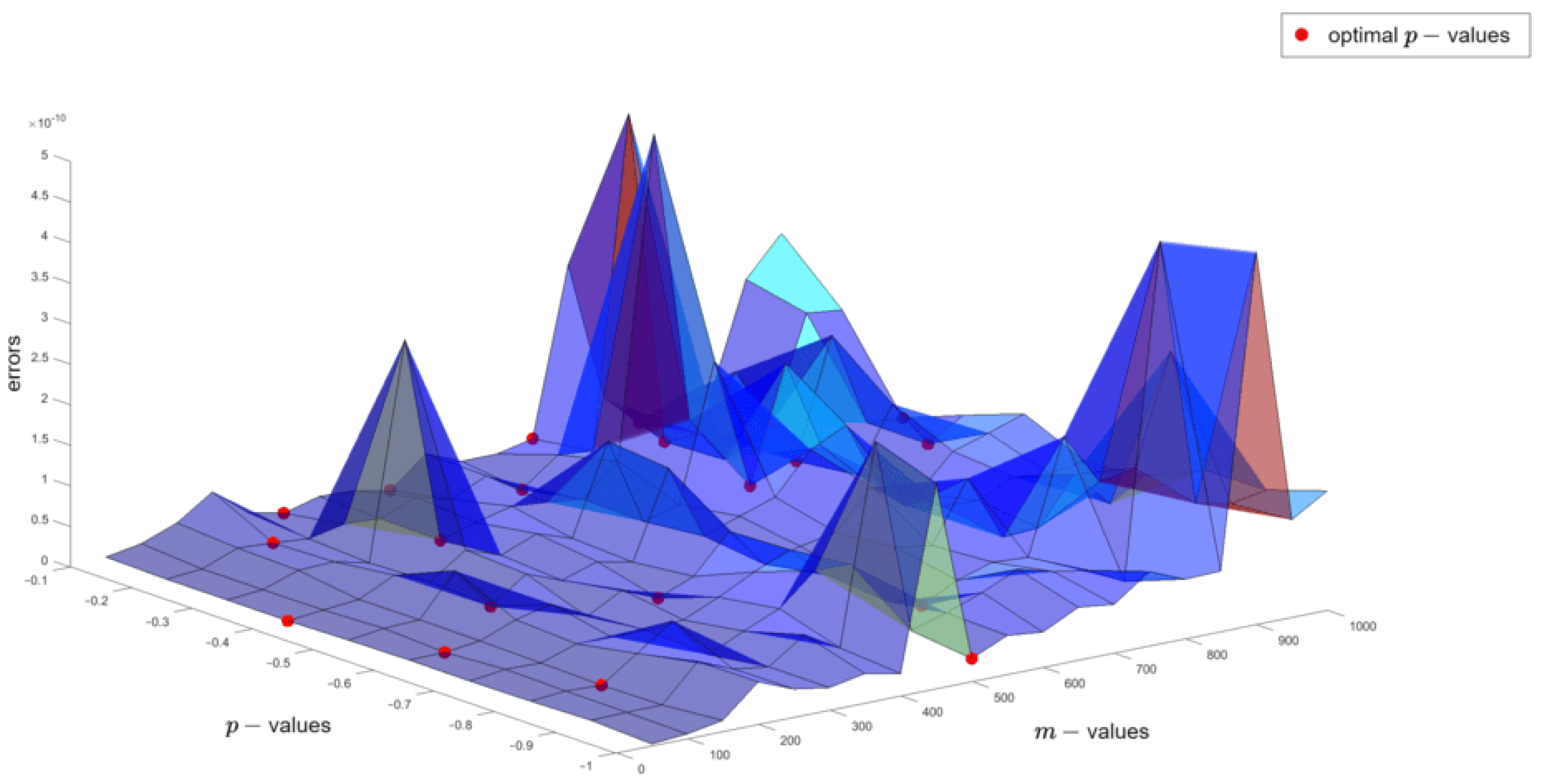
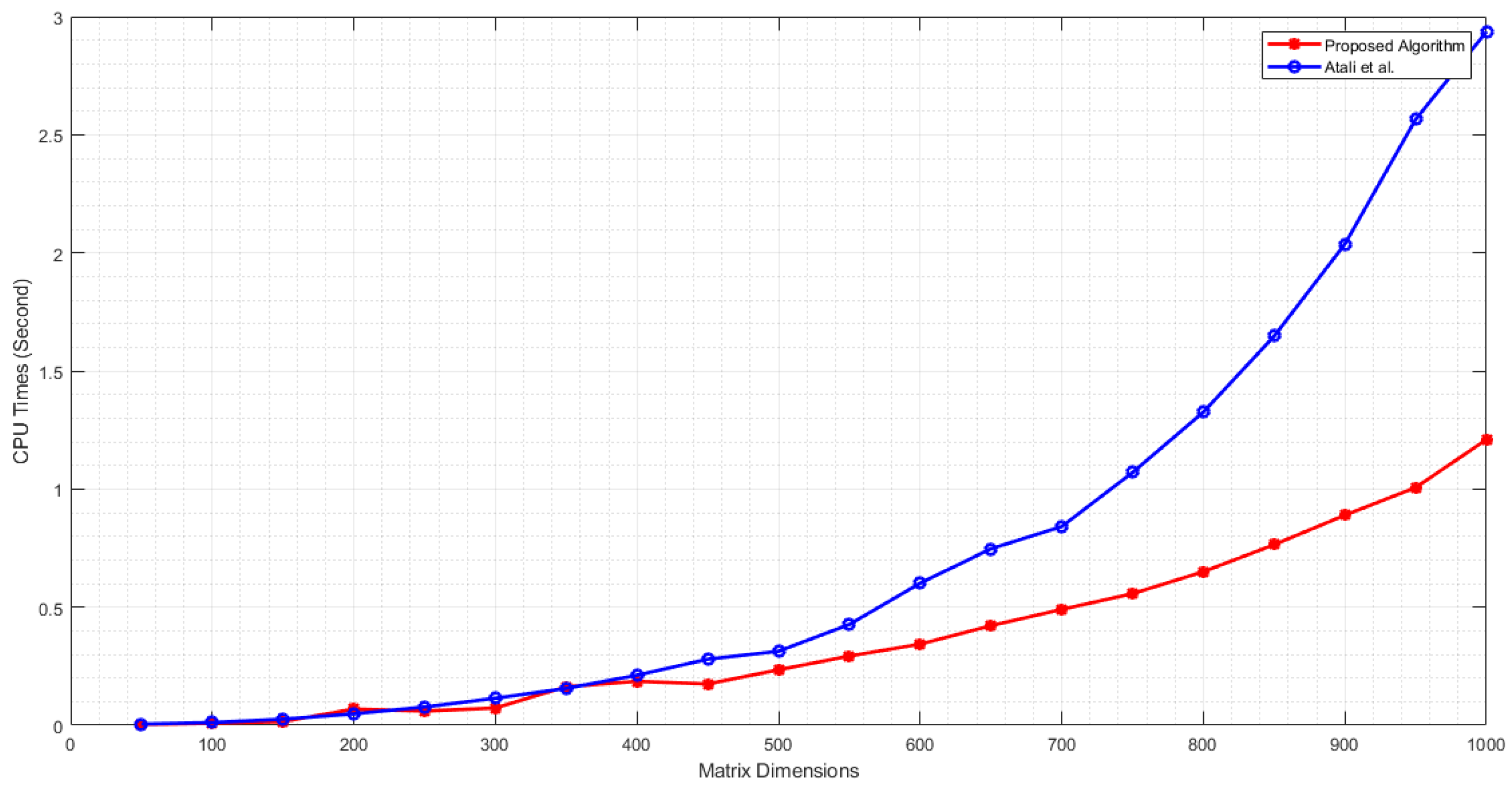
3.2.2. Numerical Examples

In this subsection, some illustrative examples are given to prove the authenticity of our results and distinguish them from existing ones. Moreover, all computations are performed using the MATLAB^® 2024a (64 bit) on an Intel(R) Xeon(R) CPU E5-1650 v4 @3.60 GHz (12 CPUs)/16 GB (DDR3) RAM computer.

Example 1.

Given the EQ matrices $Q_{1,\left(E\right)}$ and $Q_{2,\left(E\right)}$ as follows:

$$Q_{1,\left(E\right)}=\left(\begin{array}{ccc}9+i-7j+2k& 2-7i+j+5k& 8-4i+7j-4k\\ 5+8i-j+4k& 4+7i+j-k& 9-6i-3j+8k\\ 8+9i+3j-4k& 9-2i+8j+2k& 6-5i+9j-6k\end{array}\right)\in {\mathbb{H}}_{-0.5}^{3\times 3},$$

and

$$Q_{2,\left(E\right)}=\left(\begin{array}{c}7+2i+3j+k\\ 7-6i+j+4k\\ 3+3i-5j-8k\end{array}\right)\in {\mathbb{H}}_{-0.5}^{3\times 1}.$$

Let’s find the least squares solution with the minimum norm by using Algorithms 2–4 for $p=-0.5$. By the Algorithm 2, we get the singular value decomposition of EQ matrix $Q_{1,\left(E\right)}$ as follows:

$$\Sigma =\left(\begin{array}{ccc}27.1507+5.1850j& 0& 0\\ 0& 13.3956-3.6604j& 0\\ 0& 0& 3.5511+0.0727j\end{array}\right),$$

$$U=\left(\begin{array}{ccc}-0.5887-0.0895i+0.1905j-0.1797k& 0.5737+0.2198i+0.2880j-0.0213k& -0.1504-0.0811i+0.3531j+0.1408k\\ -0.2573-0.4628i+0.0895j-0.0090k& -0.2014-0.8270i+0.0050j+0.3648k& 0.1490+0.6752i+0.1013j+0.4671k\\ -0.4969-0.4443i-0.2639j+0.0273k& -0.1356+0.2676i-0.1680j-0.2529k& -0.1172+0.4220i-0.326j-0.7217k\end{array}\right),$$

and

$$V=\left(\begin{array}{ccc}-0.6674+0.2309j& -0.1204-0.3768j& 0.5534+0.1965j\\ -0.3280-0.3659i-0.1703j+0.0553k& -0.4857+0.1440i-0.0426j+0.0036k& -0.3596-0.6220i-0.2807j+0.5391k\\ -0.2692-0.5713i-0.2100j-0.1815k& 0.4859-0.3190i+0.1157j+0.7682k& -0.1476-0.1702i+0.2676j+0.0299k\end{array}\right).$$

By Algorithms 3 and 4, the least squares solution and minimum norm are found as

$$\begin{array}{cc}\hfill X_{\left(E\right)}=& Q_{1,\left(E\right)}^{†}{Q}_{2,\left(E\right)}=V_{\left(E\right)}{\Sigma }_{\left(E\right)}^{†}{U}_{\left(E\right)}^{\ast }{Q}_{2,\left(E\right)}\hfill \\ \hfill =& \left(\begin{array}{c}0.7612-1.5582i-0.1979j-0.5332k\\ -1.4757-0.2366i+0.1496j+1.2282k\\ 0.0461+0.2919i+0.4652j-0.0282k\end{array}\right)\hfill \end{array}$$

and

$${∥Q_{1,\left(E\right)}{X}_{\left(E\right)}-Q_{2,\left(E\right)}∥}_p=1.1801\times {10}^{-14},$$

respectively.

Example 2.

Let’s define the dimensions of the EQ matrices $Q_{1,\left(E\right)}$ and $Q_{2,\left(E\right)}$ given by:

$$\begin{array}{c}m=50:50:1000,\hfill \\ Q_{1,\left(E\right)}=rand\left(m,m\right)+rand\left(m,m\right)i+rand\left(m,m\right)j+rand\left(m,m\right)k,\hfill \\ Q_{2,\left(E\right)}=rand\left(m,1\right)+rand\left(m,1\right)i+rand\left(m,1\right)j+rand\left(m,1\right)k.\hfill \end{array}$$

Then, the errors (or minimum norms) corresponding p and m-values are shown in Figure 1. Here, Algorithm 4 was executed for each m-value, iterating over each p-value in the range $-1\le p\le -0.1$ with a step size of $0.1$. The minimal errors were identified and highlighted on the surface plot with red dots. Also, we compare our new proposed Algorithm 4 and the Algorithm documented by Atali et al. in [21], focusing on CPU time and error metrics. The experimental results of this comparison are depicted in Figure 2 (CPU times) and Figure 3 (Errors). Figure 2 and Figure 3 show that our proposed algorithm outperforms the algorithm presented by Atali et al. in [21] regarding computational efficiency and accuracy.

Figure 1. Errors corresponding p and m-values.

Figure 2. CPU times comparison proposed algorithm with the algorithm in [21].

Figure 3. Errors comparison proposed algorithm with the algorithm in [21].

4. Conclusions

In this study, we derived outcomes for determining eigen-pairs, performing singular value decomposition, obtaining pseudoinverse, and finding the least squares solution with the minimum norm for EQ matrices. Additionally, we developed algorithms grounded on these outcomes and presented illustrative numerical instances to validate our results. This number system is more useful in applied sciences since it allows one to select the ideal p-value suited for the type of problem, considering the elliptical behavior of many physical systems. As a result, the use of EQs in today’s critical technology fields—information security, data analytics, simulation technologies, robotics, signal processing, image processing, artificial intelligence, and machine learning—may effectively solve many problems related to time, memory, and performance.

References

- Ben-Israel, A.; Greville, T.N. Generalized Inverses: Theory and Applications; Springer Science Business Media: Berlin/Heidelberg, Germany, 2006. [Google Scholar]
- Samar, M.; Li, H.; Wei, Y. Condition numbers for the K-weighted pseudoinverse and their statistical estimation. Linear Multilinear Algebra 2021, 69, 752–770. [Google Scholar] [CrossRef]
- Samar, M.; Zhu, X.; Xu, H. Conditioning Theory for -Weighted Pseudoinverse and -Weighted Least Squares Problem. Axioms 2021, 13, 345. [Google Scholar] [CrossRef]
- Simsek, S. Least-squares solutions of generalized Sylvester-type quaternion matrix equations. Adv. Appl. Clifford Algebr. 2023, 33, 28. [Google Scholar] [CrossRef]
- Dian, R.; Li, S.; Kang, X. Regularizing hyperspectral and multispectral image fusion by CNN denoiser. IEEE Trans. Neural Netw. Learn. Syst. 2021, 32, 1124–1135. [Google Scholar] [CrossRef] [PubMed]
- Hashemipour, N.; Aghaei, J.; Kavousi-Fard, A.; Niknam, T.; Salimi, L.; del Granado, P.C.; Shafie-Khah, M.; Wang, F.; Catalão, J.P.S. Optimal Singular value decomposition based big data compression approach in smart grids. IEEE Trans. Ind. Appl. 2021, 32, 1124–1135. [Google Scholar] [CrossRef]
- Wang, Y.C.; Zhu, L. Research and implementation of SVD in machine learning. In Proceedings of the 2017 IEEE/ACIS 16th International Conference on Computer and Information Science, Wuhan, China, 24–26 May 2017; pp. 471–475. [Google Scholar]
- Harkin, A.A.; Harkin, J.B. Geometry of generalized complex numbers. Math. Mag. 2004, 77, 118–129. [Google Scholar] [CrossRef]
- Catoni, F.; Cannata, R.; Zampetti, P. An introduction to commutative quaternions. Adv. Appl. Clifford Algebr. 2006, 16, 1–28. [Google Scholar] [CrossRef]
- Yaglom, I.M. A Simple Non-Euclidean Geometry and Its Physical Basis; Springer: New York, NY, USA, 1979. [Google Scholar]
- Condurache, D.; Burlacu, A. Dual tensors based solutions for rigid body motion parameterization. Mech. Mach. Theory 2014, 74, 390–412. [Google Scholar] [CrossRef]
- Ozdemir, M. An alternative approach to elliptical motion. Adv. Appl. Clifford Algebr. 2016, 26, 279–304. [Google Scholar] [CrossRef]
- Dundar, F.S.; Ersoy, S.; Pereira, N.T.S. Bobillier formula for the elliptical harmonic motion. An. St. Univ. Ovidius Constanta 2018, 26, 103–110. [Google Scholar] [CrossRef]
- Derin, Z.; Gungor, M.A. Elliptic biquaternionic equations of gravitoelectromagnetism. Math. Methods Appl. Sci. 2022, 45, 4231–4243. [Google Scholar] [CrossRef]
- Catoni, F.; Cannata, R.; Zampetti, P. An introduction to constant curvature spaces in the commutative (Segre) quaternion geometry. Adv. Appl. Clifford Algebr. 2006, 16, 85–101. [Google Scholar] [CrossRef]
- Guo, L.; Zhu, M.; Ge, X. Reduced biquaternion canonical transform, convolution and correlation. Signal Process. 2011, 91, 2147–2153. [Google Scholar] [CrossRef]
- Yuan, S.F.; Tian, Y.; Li, M.Z. On Hermitian solutions of the reduced biquaternion matrix equation (AXB, CXD) = (E, G). Linear Multilinear Algebra 2020, 68, 1355–1373. [Google Scholar] [CrossRef]
- Tosun, M.; Kosal, H.H. An algorithm for solving the Sylvester s-conjugate elliptic quaternion matrix equations. In Algorithms as a Basis of Modern Applied Mathematics; Hošková-Mayerová, Š., Flaut, C., Maturo, F., Eds.; Springer International Publishing: Cham, Switzerland, 2021; pp. 279–292. [Google Scholar]
- Gai, S.; Huang, X. Reduced biquaternion convolutional neural network for color image processing. IEEE Trans. Circuits Syst. Video Technol. 2022, 32, 1061–1075. [Google Scholar] [CrossRef]
- Guo, Z.; Zhang, D.; Vasiliev, V.I.; Jiang, T. Algebraic techniques for Maxwell’s equations in commutative quaternionic electromagnetics. Eur. Phys. J. Plus 2022, 137, 577–1075. [Google Scholar]
- Atali, G.; Kosal, H.H.; Pekyaman, M. A new image restoration model associated with special elliptic quaternionic least-squares solutions based on LabVIEW. J. Comput. Appl. Math. 2023, 425, 115071. [Google Scholar] [CrossRef]
- Catoni, F.; Boccaletti, D.; Cannata, R.; Catoni, V.; Nichelatti, E.; Zampetti, P. The Mathematics of Minkowski Space–Time: With an Introduction to Commutative Hypercomplex Numbers; Birkhäuser: Basel, Switzerland, 2008. [Google Scholar]
- Surekci, A.; Kosal, H.H.; Gungor, M.A. A Note on Gershgorin disks in the elliptic plane. J. Math. Sci. Model. 2021, 4, 104–109. [Google Scholar]
Disclaimer/Publisher’s Note: The statements, opinions and data contained in all publications are solely those of the individual author(s) and contributor(s) and not of MDPI and/or the editor(s). MDPI and/or the editor(s) disclaim responsibility for any injury to people or property resulting from any ideas, methods, instructions or products referred to in the content. |
© 2024 by the authors. Licensee MDPI, Basel, Switzerland. This article is an open access article distributed under the terms and conditions of the Creative Commons Attribution (CC BY) license (https://creativecommons.org/licenses/by/4.0/).