Topological Comparison of Some Dimension Reduction Methods Using Persistent Homology on EEG Data

Abstract

In this paper, we explore how to use topological tools to compare dimension reduction methods. We first make a brief overview of some of the methods often used in dimension reduction such as isometric feature mapping, Laplacian Eigenmaps, fast independent component analysis, kernel ridge regression, and t-distributed stochastic neighbor embedding. We then give a brief overview of some of the topological notions used in topological data analysis, such as barcodes, persistent homology, and Wasserstein distance. Theoretically, when these methods are applied on a data set, they can be interpreted differently. From EEG data embedded into a manifold of high dimension, we discuss these methods and we compare them across persistent homologies of dimensions 0, 1, and 2, that is, across connected components, tunnels and holes, shells around voids, or cavities. We find that from three dimension clouds of points, it is not clear how distinct from each other the methods are, but Wasserstein and Bottleneck distances, topological tests of hypothesis, and various methods show that the methods qualitatively and significantly differ across homologies. We can infer from this analysis that topological persistent homologies do change dramatically at seizure, a finding already obtained in previous analyses. This suggests that looking at changes in homology landscapes could be a predictor of seizure.

1. Introduction

In topological data analysis, one is interested in understanding high dimensional structures from low dimensional ones and how discrete structures can be aggregated to form a global structure. It can be a difficult task to even think or believe that high dimensional objects exist beyond three dimensions since we can not visualize objects beyond a three-dimensional space. However, embedding theorems clearly show that these high dimension structures do, in fact, exist, for instance, Whitney [1] and Takens [2] embedding theorems. From a practical point of view, to make inferences on structures embedded in high dimensional ambient spaces, some kind of dimensional reduction needs to occur. From a data analysis point of view, dimension reduction amounts to data compression where a certain amount of information may be lost. This dimension reduction is part of manifold learning, which can be understood as a collection of algorithms for recovering low dimension manifolds embedded into high dimensional ambient spaces while preserving meaningful information, see Ma and Fu [3]. The algorithms for dimension reduction may be classified into linear and nonlinear methods or parametric or nonparametric methods, where the goal is to select or extract coarse features from high dimensional data. Among the pioneering linear methods is the principal component analysis (PCA) introduced by Hotelling in [4]. Its primary goal is to reduce the data to a set of orthogonal linear projections ordered by decreasing variances. Another linear method is multidimensional scaling (MSD), where the data are aggregated using a measure of proximity, which could be a distance or a measure of association such as correlation or any other method describing how close entities can be, see, for instance, Ramsey and Silverman [5]. Linear discriminant analysis (LDA) is a linear method similar to PCA consisting of writing a categorical dependent variable as a linear combination of continuous independent variables, see, for instance, Cohen et al. [6], Friedman [7], or Yu and Yang [8]. As such, it is opposite to an analysis of variance (ANOVA) where the dependent variable is continuous and the independent variables are categorical. The focus of this paper will be on nonlinear techniques, which, similar to their linear counterparts, aim to extract or select low dimensional features while preserving important information. Since there are many such methods, our focus will be on isometric feature mapping (ISOMAP) [9], Laplacian Eigenmaps [10], fast independent component analysis, (Fast-ICA) [11], kernel ridge regression [12], and t-distributed stochastic neighbor embedding (t-SNE) [13]. We will compare them using persistent homology (PH). PH is one the many techniques of topological data analysis (TDA) that can be used to identify features in data that remain persistent over multiple and different scales. This tool can provide new insights into seemingly known or unknown data and has the potential to uncover interesting hidden information embedded within data. For instance, PH was used to provide new insights on the topology of deep neural networks, see [14]. PH was successfully used to provide new perspectives on viral evolution, see [15]. The following examples of successful applications can be found in [16], including but not limited to better understanding of sensor-network coverage, see [17]; proteins, see [18,19]; dimensional structure of DNA, see [20]; cell development, see [21]; robotics, see [22,23,24]; signal processing, see [25,26]; spread of contagions, see [27]; financial networks, see [28]; applications in neuroscience, see [29,30]; time-series output of dynamical systems, see [31]; and EEG epilepsy, see [32]. The approach in the last reference is of particular interest to us. Indeed, in that paper, the authors considered the EEG measured in a healthy person during sleep. They used the method of false nearest neighbors to estimate the embedding dimension. From there, persistent barcode diagrams were obtained and revealed that topological noise persisted at certain dimensions and vanished at some others. This paper has a similar approach and is organized as follows: in Section 2, we review theories behind some dimension reduction methods; then, in Section 3, we give an overview of the essentials of persistent homology; in Section 4, we discuss how to apply persistent homology to the data and compare the methods on an EEG data set using persistent homology. Finally. in Section 5, we make some concluding remarks.

2. Materials and Methods

Let us note that some of the review methods below are extensively described in [3]. To have all of our ideas self-contained, we reintroduce a few concepts. In the sequel, $∥·∥$ is the euclidian norm in ${\mathbb{R}}^d$, for some $d\ge 3$. In the sequel, topological spaces $\mathcal{M}$ will considered to be second-countable Hausdorff; that is, (a) every pair of distinct points has a corresponding pair of disjoint neighborhoods. (b) Its topology has a countable basis of open sets. This assumption is satisfied in most topological spaces and seems reasonable.

2.1. Preliminaries

Definition 1. 

A topological space $\mathcal{M}$ is called a (topological) manifold if, locally, it resembles a real n-dimensional Euclidian space, that is, there exists $n\in \mathbb{N}$ such that for all $x\in \mathcal{M}$, there exists a neighborhood $U_x$ of x and a homeomorphism $f:U_x\to {\mathbb{R}}^n$. The pair $(U_x,f)$ is referred to as a chart on $\mathcal{M}$ and f is called a parametrization at x.

Definition 2. 

Let $\mathcal{M}$ be a manifold. $\mathcal{M}$ is said to be smooth if given $x\in \mathcal{M}$, the parametrization f at x has smooth or continuous partial derivatives of any order and can be extended to a smooth function $F:\mathcal{M}\to {\mathbb{R}}^n$ such that $F{|}_{\mathcal{M}\cap U_x}=f$.

Definition 3. 

Let $\mathcal{M}$ and $\mathcal{N}$ be differentiable manifolds. A function $\psi :\mathcal{M}\to \mathcal{N}$ is an embedding if ψ is an injective immersion.

Next, we introduce the notion of the boundary of the topological manifold, which will be important in the sequel.

Definition 4. 

Consider a Hausdorff topological manifold $\mathcal{M}$ homeomorphic to an open subset of the half-euclidian space ${\mathbb{R}}_{+}^n$. Let the interior $Int\left(\mathcal{M}\right)$ of $\mathcal{M}$ be the subspace of $\mathcal{M}$ formed by all points s that have a neighborhood homeomorphic to ${\mathbb{R}}^n$. Then, the boundary of $\mathcal{M}$ is defined as a complement of $Int\left(\mathcal{M}\right)$ in $\mathcal{M}$, that is, $\mathcal{M}\setminus Int\left(\mathcal{M}\right)$, which is an $n-1$-dimensional topological manifold.

2.2. ISOMAP

Isometric feature mapping (ISOMAP) was introduced by Tanenbaum et al. in [9]. The data are considered to be a finite sample $\left\{{\mathit{v}}_i\right\}$ from a smooth manifold $\mathcal{M}$. The two key assumptions are: (a) an isometric embedding $\psi :\mathcal{M}\to \mathcal{X}$ exists where $\mathcal{X}={\mathbb{R}}^d$, where the distance on $\mathcal{M}$ is the geodesic distance or the shortest curve connecting two points; (b) the smooth manifold $\mathcal{M}$ is a convex region of ${\mathbb{R}}^m$, where $m<<d$. The implementation phase has three main steps.

1.

For a fixed integer K and real number $ϵ>0$, perform an $ϵ-K$-nearest neighbor search using the fact that the geodesic distance $D^{\mathcal{M}}(v_i,v_j)$ between two points on $\mathcal{M}$ is the same (by isometry) as their euclidian distance $∥v_i-v_j∥$ in ${\mathbb{R}}^d$. K is the number of data points selected within a ball of radius $ϵ$.

2.

Having calculated the distance between points as above, the entire data set can be considered as a weighted graph with vertices $\mathit{v}=\left\{v_i\right\}$ and edges $\mathit{e}=\left\{e_{ij}\right\}$, where $e_{ij}$ connects $v_i$ with $v_j$ with a distance $w_{ij}=D^{\mathcal{M}}(v_i,v_j)$, considered an associated weight. The geodesic distance between two data points $v_i$ and $v_j$ is estimated as the graph distance between the two edges, that is, the number of edges in the shortest path connecting them. We observe that this shortest path is found by minimizing the sum of the weights of its constituent edges.

3.

Having calculated the geodesic distances $D^G=\left\{w_{ij}\right\}$ as above, we observe that $D^G$ is a symmetric matrix, so we can apply the classical multidimensional scaling algorithm (MDS) (see [33]) to $D^G$ by mapping (embedding) them into a feature space $\mathcal{Y}$ of dimension d while preserving the geodesic distance on $\mathcal{M}$. $\mathcal{Y}$ is generated by a $d\times m$ matrix whose i-th column represents the coordinates of $v_i$ in $\mathcal{Y}$.

2.3. Laplacian Eigenmaps

The Laplacian Eigenmaps (LEIM) algorithm was introduced by Belkin and Niyogi in [10]. As above, the data $\mathit{v}=\left\{v_i\right\}$ are supposed to be from a smooth manifold $\mathcal{M}$. It also has three main steps:

1.

For a fixed integer K and real number $ϵ>0$, perform a K-nearest neighbor search on symmetric neighborhoods. Note that given two points $v_i,v_j$, their respective K-neighborhood $N_i^K$ and $N_j^K$ are symmetric if and only $v_i\in N_j^K⟺v_j\in N_i^K$.

2.

For a given real number $\sigma >0$ and each pair of points $(v_i,v_j)$, calculate the weight $w_{ij}=e^{-\frac{{∥u_i-v_j∥}^2}{2{\sigma }^2}}$ if $v_i\in N_j^K$ and $w_{ij}=0$ if $v_i\notin N_j^K$. Obtain the adjacency matrix $\mathit{W}=\left(w_{ij}\right)$. The data now form a weighted graph with vertices $\mathit{v}$, with edges $\mathit{e}=\left\{e_{ij}\right\}$, and weights $\mathit{W}=\left\{w_{ij}\right\}$, where $e_{ij}$ connects $v_i$ with $v_j$ with distance $w_{ij}$.

3.

Consider $\mathbf{\Lambda }=\left\{{\lambda }_{ij}\right\}$ to be a diagonal matrix with ${\displaystyle {\lambda }_{ii}=\sum _j{w}_{ij}}$ and define the graph Laplacian as $\mathit{L}=\mathbf{\Lambda }-\mathit{W}$. Then, $\mathit{L}$ is positive definite so let $\widehat{\mathit{Y}}$ be the $d\times n$ matrix that minimizes ${\displaystyle \sum _{i,j}{w}_{ij}{∥{\mathbf{y}}_i-{\mathbf{y}}_j∥}^2=tr\left({\mathit{TLY}}^{\mathit{T}}\right)}$. Then, $\widehat{\mathbf{Y}}$ can used to embed $\mathcal{M}$ into a d-dimensional space $\mathcal{Y}$, whose i-th column represents the coordinates of $v_i$ in $\mathcal{Y}$.

2.4. Fast ICA

The fast independent component analysis (Fast-ICA) algorithms were introduced by Hyvärinen in [11]. As above, the data $\mathit{v}$ are considered to be from a smooth manifold $\mathcal{M}$. It is assumed that the data $\mathit{v}$ are represented as an $n\times m$ matrix $\left(v_{ij}\right)$ that can be flattened into a $n\times m$ vector. As in principal component analysis (PCA), in factor analysis, projection pursuit, or independent component analysis (ICA), by considering the data as an $n\times m$-dimensional observed random variable, the goal is to determine a matrix $\mathit{W}$ such that $\mathit{s}={\mathit{W}}^{\mathit{T}}\mathit{v}$, where $\mathit{s}$ is a $n\times m$-dimensional random variable having desirable properties such as optimal dimension reduction or other interesting statistical properties such as minimal variance. Optimally, the components of $\mathit{s}$ should provide source separation (the original data source $\mathit{v}$ is assumed to be corrupted with noise) and feature extraction and be independent of each other. In a regular ICA, the matrix $\mathit{W}$ is found by minimizing the mutual information, a measure of dependence between given random variables. In fast-ICA algorithms, the matrix $\mathit{W}$ is found by using a Newton fixed point approach, with an objective function taken as the differential entropy, given as $J_G\left(\mathit{W}\right)={\left(\mathbb{E}\left[G\left({\mathit{W}}^{\mathit{T}}\mathit{W}\right)\right]-\mathbb{E}\left[G\left(z\right)\right]\right)}^2$, where it is assumed that $\mathit{W}$ is such that $\mathbb{E}\left[{\left({\mathit{W}}^{\mathit{T}}\mathit{W}\right)}^2\right]=1$, and z is the standard normal distribution. G is a function referred to as the contrast function, which includes but is not limited to $G\left(u\right)={\alpha }^{-1}log(cosh\left(\alpha u\right)),G\left(u\right)=-{\sigma }^{-1}{e}^{-0.5\sigma u^2},G\left(u\right)=0.25u^4$, where $\alpha \in [1,2]$ and $\sigma \approx 1$. From a dynamical system point of view, the fixed point is locally asymptotically stable with the exception of $G\left(u\right)=0.25u^4$, where stability becomes global. For simplification purposes, let $g\left(x\right)=G^{\prime }\left(x\right)$. The key steps are:

1.

Data preparation: it consists of centering the data $\mathit{v}$ with respect to the column to obtain ${\mathit{v}}^c$. That is, ${\displaystyle v_{ij}^c=v_{ij}-\frac{1}{m}\sum _{j=1}^m{v}_{ij}}$, for $i=1,2,\cdots ,n$. The centered data are then whitened; that is, ${\mathit{v}}^c$ is linearly transformed into ${\mathit{v}}_w^c$, a matrix of uncorrelated components. This is accomplished through an eigenvalue decomposition of the covariance matrix $\mathit{C}={\mathit{v}}^{\mathit{c}}{\left({\mathit{v}}^{\mathit{c}}\right)}^{\mathit{T}}$ to obtain two matrices $\mathit{V},\mathit{E}$, respectively, of eigenvectors and eigenvalues so that $\mathbb{E}\left[\mathit{C}\right]={\mathit{VEV}}^{\mathit{T}}$. The whitened data are found as ${\mathit{v}}_{\mathit{w}}^{\mathit{c}}={\mathit{E}}^{-\mathbf{1}/\mathbf{2}}{\mathit{V}}^{\mathit{T}}{\mathit{v}}^{\mathit{c}}$ and simply referred to again as $\mathit{v}$ for simplicity.

2.

Component extraction: Let $F\left(\mathit{W}\right)=\mathbb{E}\left[\mathit{v}g\left({\mathit{W}}^{\mathit{T}}\mathit{v}\right)\right]-\beta \mathit{W}$ for a given constant $\beta =\mathbb{E}\left[{\mathit{W}}_{\mathit{a}}^{\mathit{T}}\mathit{v}g\left({\mathit{W}}_{\mathit{a}}^{\mathit{T}}\mathit{v}\right)\right]$, where $W_a$ is the optimal weight matrix. Applying the Newton scheme ($x_{n+1}=x_n-F\left(x_n\right){\left[F^{\prime }\left(x_n\right)\right]}^{-1}$) to the differentiable function $J_G$, we

• Select a random starting vector ${\mathit{W}}_0$.
• For $n\ge 0$, ${\mathit{W}}_{n+1}=\mathbb{E}\left[\mathit{v}g\left({\mathit{W}}_n^T\mathit{v}\right)\right]-\mathbb{E}\left[g^{\prime }\left({\mathit{W}}_n^T\mathit{v}\right)\right]{\mathit{W}}_n$.
• Normalize ${\mathit{W}}_{n+1}$ as ${\displaystyle \frac{{\mathit{W}}_{n+1}}{∥{\mathit{W}}_{n+1}∥}}$.
• Repeat until a suitable convergence level is reached.
• From the last matrix $\mathit{W}$ obtained, let $\mathit{s}={\mathit{W}}^{\mathit{T}}\mathit{v}$.

2.5. Kernel Ridge Regression

The kernel ridge regression (KRR) is constructed as follows: as above, the data $\mathit{v}$ are considered to be from a smooth manifold $\mathcal{M}$ of dimension d. It is assumed that the data $\mathit{v}$ are represented as an $n\times m$ matrix $\left\{v_{ij}\right\}$ that can be flattened into a $n\times m$ vector. Suppose we are in possession of $\mathit{u}=(u_1,u_2,\cdots ,u_n)$ data corresponding to a response variable and covariates given as $\mathit{v}=\left({\mathit{v}}_{\mathbf{1}},{\mathit{v}}_{\mathbf{2}},\cdots ,{\mathit{v}}_{\mathbf{n}}\right)$, where ${\mathit{v}}_{\mathbf{i}}={\left(v_{ij}\right)}^T$ for $j=1,2,\cdots ,m$. With the least square method, we can find the best linear model between the covariates $\mathit{v}=\left(v_i\right)$ and the response $\mathit{u}=\left(u_i\right)$ by minimizing the objective function ${\displaystyle L\left(\mathit{W}\right)=\frac{1}{2}\sum _{i=1}^L{(u_i-{{\mathit{W}}^{\mathit{T}}\mathit{v}}_i)}^2}$, where $\mathit{W}$ is a $1\times n$ vector. Similar approaches include maximum likelihood approaches, see, for instance, [34] or perpendicular offsets [35]. However, regression methods are notorious for overfitting. Overfitting occurs when a model closely fits a training data set but fails to do so on a test data set. In practice, this can lead to dire consequences, see, for instance, the book by Nate Silver [36] for illustrative examples in real life. Numerous solutions were proposed to overcome overfitting; these include but are not limited to training with more data, data augmentation, cross-validation, feature selection, regularization, or penalization (Lasso, Ridge, Elastic net). The ridge regression is a compromise that uses a penalized objective function such as ${\displaystyle L\left(\mathit{W}\right)=\frac{1}{2}\sum _{i=1}^L{(u_i-{{\mathit{W}}^{\mathit{T}}\mathit{v}}_i)}^2+\frac{\lambda }{2}{∥\mathit{W}∥}^2}$. The solution can be found as ${\displaystyle \mathit{W}={\left(\lambda I+\sum _{i=1}^n{{\mathit{v}}_{\mathbf{i}}{\mathit{v}}_{\mathbf{i}}}^T\right)}^{-1}\left(\sum _{i=1}^n{u}_i{\mathit{v}}_i\right)}$. In case the true nature of the relationship between the response and covariates is nonlinear, we can replace ${\mathit{v}}_i$ with $\phi \left({\mathit{v}}_i\right)$, where $\phi$ is a nonlinear function ${\mathbb{R}}^m\to \mathbb{R}$. In particular, if the response is qualitative, that is, labels, then we have a classification problem, and $\phi$ is referred to as a feature map. Note that when using $\phi$, the number of dimensions of the problem is considerably high. Put $\Phi =\phi \left(\mathit{v}\right)=(\phi \left(v_1\right),\phi \left(v_2\right),\cdots ,\phi \left(v_n\right))$. Replacing ${\mathit{v}}_{\mathbf{i}}$ with $\phi \left({\mathit{v}}_{\mathbf{i}}\right)$, the solution above becomes ${\displaystyle \mathit{W}={\left(\lambda I+\sum _{i=1}^n\phi \left({\mathit{v}}_{\mathit{i}}\right)\phi {\left({\mathit{v}}_{\mathit{i}}\right)}^T\right)}^{-1}\left(\sum _{i=1}^n{u}_i\phi \left({\mathit{v}}_i\right)\right)={(\lambda I+\Phi {\Phi }^T)}^{-1}\Phi {\mathit{u}}^T}$. Consider the following identity $A{B}^T{(C+BA{B}^T)}^{-1}={(A^{-1}+B^T{C}^{-1}B)}^{-1}{B}^T{C}^{-1}$ for the given invertible matrices $A,C$, and a matrix B. Applying this with $A=C=I$ and $B=\Phi$, we have ${\mathit{W}}^{\mathit{T}}=\mathit{u}\left[{\Phi }^T{(\lambda I+{\Phi }^T\Phi )}^{-1}\right]=\mathit{u}\left[{(\lambda I+{\Phi }^T\Phi )}^{-1}{\Phi }^T\right]$. Therefore, given a new value ${\mathit{v}}_n$, the predicted value is $y_n={\mathit{W}}^T\Phi \left({\mathit{v}}_n\right)=\mathit{u}{({\Phi }^T\Phi +\lambda I)}^{-1}{\Phi }^T\Phi \left({\mathit{v}}_n\right)=\mathit{u}{(K+\lambda I)}^{-1}\kappa \left({\mathit{v}}_n\right)$, where ${\displaystyle K=K({\mathit{v}}_i,{\mathit{v}}_i)={\Phi }^T\Phi =\sum _{i=1}^n\phi {\left({\mathit{v}}_i\right)}^T\phi \left({\mathit{v}}_i\right)}$ and $\kappa \left({\mathit{v}}_n\right)=K({\mathit{v}}_i,{\mathit{v}}_n)$. K is referred to as the kernel, which is the only quantity needed to be calculated, thereby significantly reducing the computational time and dimensionality of the problem. In practice, we may use a linear kernel $K(\mathit{x},\mathit{y})={\mathit{x}}^T\mathit{y}$ or a Gaussian kernel $K(\mathit{x},\mathit{y})=e^{-\sigma {∥\mathit{x}-\mathit{y}∥}^2}$, for some $\sigma >0$, where $∥·∥$ is a norm in ${\mathbb{R}}^m$ and $\sigma$ is given a real constant.

2.6. t-SNE

Stochastic neighbor embedding (SNE) was proposed by Hinston and Roweis in [37]. t-SNE followed later and was proposed by van der Maaten and Hinton in [13]. t-distributed stochastic neighbor embedding (t-SNE) is a dimension reduction method that amounts to assigning data to two or three dimensional maps. As above, we consider the data $\mathit{v}=\left(v_{ij}\right)=\left(v_k\right)$ ($k=1,2,\cdots ,N$ with $N=n\times m$) to be from a smooth manifold $\mathcal{M}$ of high dimension, d. The main steps of the method are:

• Calculate the asymmetrical probabilities $p_{kl}$ as $p_{kl}=\frac{e^{-{\delta }_{kl}}}{{\sum }_{k\ne l}{e}^{-{\delta }_{kl}}}$, where ${\delta }_{kl}=\frac{{∥v_k-v_l∥}^2}{2{\sigma }_i}$ represents the dissimilarity between $v_k$ and $v_l$, and ${\sigma }_i$ is a parameter selected by the experimenter or by a binary search. $p_{kl}$ represents the conditional probability that datapoint $v_l$ is the neighborhood of datapoint $v_k$ if neighbors were selected proportionally to their probability density under a normal distribution centered at $v_k$ and variance ${\sigma }_i$.
• Assuming that the low dimensional data are $\mathit{u}=\left(u_k\right),k=1,2,\cdots ,N$, the corresponding dissimilarity probabilities $q_{kl}$ are calculated under constant variance as $q_{kl}=\frac{e^{-d_{kl}}}{{\sum }_{k\ne l}{e}^{-d_{kl}}}$, where $d_{kl}={∥u_k-u_l∥}^2$ in the case of SNE, and ${\displaystyle q_{kl}=\frac{{(1+d_{kl})}^{-1}}{{\sum }_{k\ne l}{(1+d_{kl})}^{-1}}}$ for t-SNE.
• Then, we minimize the Kullback–Leibler divergence between $p_{kl}$ and $q_{kl}$, given as ${\displaystyle L=\sum _{k=1}^N\sum _{l=1}^N{p}_{kl}log\left(\frac{p_{kl}}{q_{kl}}\right)}$, using the gradient descent method with a momentum term with the scheme ${\displaystyle {\mathit{w}}^t={\mathit{w}}^{t-1}+\eta \frac{\partial L}{\partial \mathit{u}}+\alpha \left(t\right)({\mathit{w}}^{t-1}-{\mathit{w}}^{t-2})}$ for $t=2,3,\cdots ,T$ for some given T. Note that ${\mathit{w}}^0=(u_1,u_2,\cdots ,u_N)\sim N(0,{10}^{-4}\mathit{I})$, where $\mathit{I}$ is the $N\times N$ identity matrix, $\eta$ is a constant representing a learning rate, and $\alpha \left(t\right)$ is t-th momentum iteration. We note that ${\displaystyle \frac{\partial L}{\partial \mathit{u}}=\left(\frac{\partial L}{\partial u_k}\right)}$ for $k=1,2,\cdots ,N$ where ${\displaystyle \frac{\partial L}{\partial u_k}=4\sum _{l=1}^N(p_{kl}-q_{kl})(u_k-u_l){(1+d_{kl})}^{-1}.}$
• Then, we use $\mathit{u}={\mathit{w}}^T$ as the low dimensional representation of $\mathit{v}$.

3. Persistent Homology

In the sequel, we will introduce the essential ingredients needed to understand and compute persistent homology.

3.1. Simplex Complex

Definition 5. 

A real d-simplex S is a topological manifold of dimension d that represents the convex hull of $d+1$ points. In other words:

$$S=\left\{(t_0,t_1,\cdots ,t_d)\in {\mathbb{R}}^d:t_i\ge 0{\displaystyle and\sum _{i=1}^d{t}_i=1}\right\}.$$

(1)

Example 1. 

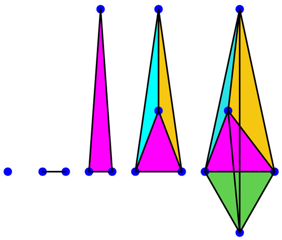
A 0-simplex is a point, a 1-simplex is an edge, a 2-simplex is a triangle, a 3-simplex is a tetrahedron, a 4-simplex is a pentachoron, etc., see for instance Figure 1 below.

Figure 1. Anillustration of 0, 1, 2, 3, and 4-simplices.

Remark 1. 

We observe that a d-simplex S can also be denoted as

$$S=[V_0,V_1,\cdots ,V_d],where V_i=\left\{vertices of V_i\right\},i=0,1,\cdots ,d.$$

We also note that the dimension of $V_i$ is i.

Definition 6. 

Given a simplex S, a face of S is another simplex R such that $R\subseteq S$ and such that the vertices of R are also the vertices of S.

Example 2. 

Given a 3-simplex (a tetrahedron), it has 4 different 2-simplex or 2 dimensional faces, each of them with three 1-simplex or 1-dimensional faces, each with three 0-simplex or 0-dimensional faces.

Definition 7. 

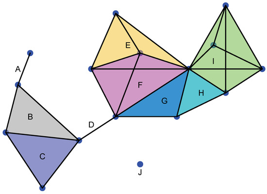
A simplicial complex Σ is a topological space formed by different simplices not necessarily of the same dimension that have to satisfy the gluing condition, that is (see Figure 2):

Figure 2. Example of a simplicial complex. J is 0-simplex; A and D are 1-simplices; B, C, G, and H are 2-simplices; E and F are 3-simplices; and I is a 4-simplex. We note that A∩ B is a 0-simplex. B∩ C is a 1-simplex and a face of B and C, respectively. E∩ F is a 2-simplex and a face of E and F. G∩ H is a 1-simplex and I∩ H is a 1-simplex.

1. 

Given $S_i\in \Sigma$, its face $R_i\in \Sigma$.

2. 

Given $S_i,S_j\in \Sigma$, either $S_i\cap S_j=\varnothing$ or $S_i\cap S_j=R_i=R_j$, the faces of $S_i$ and $S_j$, respectively.

It is important to observe that a simplicial complex can be defined very abstractly. Indeed,

Definition 8. 

A simplicial complex $\Sigma =\left\{S:S\subseteq \Omega \right\}$ is a collection of non-empty subsets of a set Ω such that

1. 

For all $\omega \in \Omega$, then $\left\{\omega \right\}\in \Sigma$.

2. 

For any set U such that $S\subset U$ for some $S\in \Sigma$, then $U\in \Sigma$.

Example 3. 

We illustrate the definition above by constructing two simplicial complexes. Let $\Omega =\left\{1,2,3,4\right\}$. We can define the following simplicial complexes on Ω.

1. 

${\displaystyle {\Sigma }_1=\left\{\left\{1\right\},\left\{2\right\},\left\{3\right\},\left\{4\right\},\left\{1,2\right\},\left\{1,3\right\},\left\{2,3\right\},\left\{1,2,3\right\}\right\}.}$

2. 

${\Sigma }_2=\mathcal{P}(\Omega )\setminus \left\{\varnothing \right\}$, where $\mathcal{P}(\Omega )$ is the set of all subsets of Ω.

3.2. Homology and Persistent Homology

Definition 9. 

Let Σ be a simplicial complex.

We define the Abelian group generated by the j-simplices of Σ as $C_j(\Sigma )$.

We define a boundary operator associated with $C_j(\Sigma )$ as a homeomorphism

$${\partial }_j:C_j(\Sigma )\to C_{j-1}(\Sigma ).$$

We define the chain complex associated with Σ as the collection of pairs

$$C(\Sigma )=\left\{(C_j(\Sigma ),{\partial }_j),j\in \mathbb{Z}\right\}.$$

Now, we can define a homology group associated with a simplicial complex.

Definition 10. 

Given a simplicial complex Σ, put $A_j(\Sigma ):=kern\left({\partial }_j\right)$ and $B_j(\Sigma ):=Im\left({\partial }_{j+1}\right)$. Then, the jth homology group ${\mathbb{H}}_j(\Sigma )$of Σ is defined as the quotient group between $A_j(\Sigma )$ and $B_j(\Sigma )$; that is,

$${\mathbb{H}}_j(\Sigma )=\frac{A_j(\Sigma )}{B_j(\Sigma )}.$$

What this reveals is the presence of “holes” in a given shape.

Remark 2. 

It is important to observe that ${\displaystyle {\mathbb{H}}_j(\Sigma )=\frac{<j-dimensionalcycles>}{<j-dimensionalboundaries>}}$, where $<U>$ stands for the span of U, and a cycle is simply a shape similar to a loop but necessarily without a starting point.

Another important remark is that the boundary operator can indeed be defined as

$${\partial }_j(\Sigma ):=\sum _{k=0}^j{(-1)}^k[V_0,\cdots ,{\widehat{V}}_k,\cdots ,V_j],$$

where ${\widehat{V}}_k$ means not counting the vertices of $V_k$. This shows that ${\partial }_j(\Sigma )$ lies in a $j-1$-simplex.

Another remark is that ${\partial }_{j-1}\circ {\partial }_j=0$ for $0\le j\le d$.

Now that we know that homology reveals the presence of “holes”, we need to find a way of determining how to count these “holes”.

Definition 11. 

Given a simplicial complex Σ, the jth Betti number $b_j(\Sigma )$ is the rank of ${\mathbb{H}}_j(\Sigma )$ or

$$b_j(\Sigma )=dim\left(A_j(\Sigma )\right)-dim\left(B_j(\Sigma )\right).$$

In other words, it is the smallest cardinality of a generating set of the group ${\mathbb{H}}_j(\Sigma )$.

In fact, since the elements of $A_j(\Sigma )$ are j-dimensional cycles and that of $B_j(\Sigma )$ are j-dimensional boundaries, the Betti number counts the number of independent j-cycles not representing the boundary of any collection of simplices of Σ.

Example 4. 

Let us be more precise by giving the meaning of the Betti number for three indices $j=0,1,2$.

1. 

$b_0$ is the number of connected components of the complex.

2. 

$b_1$ is the number of tunnels and holes.

3. 

$b_2$ is the number of shells around cavities or voids.

Definition 12. 

Let Σ be the simplicial complex, and let N be a positive integer. A filtration of Σ is a nested family ${\Sigma }_N^F:=\left\{{\Sigma }_p,0\le p\le N\right\}$ of sub-complexes of Σ such that

$${\Sigma }_0\subseteq {\Sigma }_1\subseteq {\Sigma }_2\subseteq \cdots \subseteq {\Sigma }_N=\Sigma .$$

Now, let ${\mathbb{F}}_2$ be the field with two elements, and let $0\le p\le q\le N$ be two integers.

Since ${\Sigma }_p\subseteq {\Sigma }_q$, the inclusion map $Inc{l}_{pq}:{\Sigma }_p\to {\Sigma }_q$ induces an ${\mathbb{F}}_2$-linear map defined as $g_{pq}:{\mathbb{H}}_j\left({\Sigma }_p\right)\to {\mathbb{H}}_j\left({\Sigma }_q\right)$. We can now define, for any $0\le j\le d$, the j-th persistent homology of a simplicial complex $\Sigma$.

Definition 13. 

Consider a simplicial complex Σ with filtration ${\Sigma }_N^F$ for some positive integer N. The j-th persistent homology ${\mathbb{H}}_j^{p\to q}(\Sigma )$ of Σ is defined as the pair:

$${\mathbb{H}}_j^{p\to q}(\Sigma ,{\mathbb{F}}_2):=(\left\{{\mathbb{H}}_j\left({\Sigma }_p\right),0\le p\le N\right\},\left\{g_{pq},0\le p\le q\le N\right\}).$$

In a sense, the j-th persistent homology provides more refined information than the homology of the simplicial complex in that it informs us of the changes in features such as connected components, tunnels and holes, and shells around voids through the filtration process. It can be visualized using a “barcode” or a persistent diagram. The following definition is borrowed from [38]:

Definition 14. 

Consider a simplicial complex Σ, a positive integer N, and two integers $0\le p\le q\le N$. The barcode of the j-th persistent homology ${\mathbb{H}}_j^{p\to q}(\Sigma ,{\mathbb{F}}_2)$ of Σ is a graphical representation of ${\mathbb{H}}_j^{p\to q}(\Sigma ,{\mathbb{F}}_2)$ as a collection of horizontal line segments in a plane whose horizontal axis corresponds to a parameter and whose vertical axis represents an arbitrary ordering of homology generators.

We finish this section with the introduction of the Wasserstein and Bottleneck distances, used for the comparison of persistent diagrams.

Definition 15. 

Let X and Y be two diagrams. A matching η between X and Y is a collection of pairs $\eta =\left\{(x,y)\in X\times Y\right\}$ where x and y can occur in at most one pair. It is sometimes denoted as $\eta :X\to Y$. x and y are referred to as intervals of X and Y respectively.

Example 5. 

Suppose $X=\left\{(0,1),[0,1),(0,1)\right\}$ and $Y=\left\{(-\pi ,0],(0,2)\right\}$.

Then, $\eta =\left\{\left(\right(0,1),(-\pi ,0\left]\right)\right\}$ is matching between X and Y such that $(0,1)$ is matched to $(-\pi ,0])$ and $[0,1),(0,1)$, and $(0,2)$ are unmatched.

Definition 16. 

Let $p>1$ be a real number. Given two persistent diagrams X and Y, the p-th Wasserstein distance $W_p(X,Y)$ between X and Y is defined as

$$W_p(X,Y):=\underset{\eta :X\to Y}{inf}\sum _{x\in X}{∥x-\eta \left(x\right)∥}_{\infty }^p,$$

where η is a perfect matching between the intervals of X and Y.

The Bottleneck distance is obtained when $p=\infty$; that is, it is given as

$$W_{\infty }(X,Y):=\underset{\eta :X\to Y}{inf}\underset{x\in X}{sup}{∥x-\eta \left(x\right)∥}_{\infty }.$$

4. Results

In the presence of data, simplicial complexes will be replaced by sets of data indexed by a parameter, therefore, transforming these sets into parametrized topological entities. On these parametrized topological entities, the notions of persistent homology introduced above can be computed, especially the Betti number, in the form of a “barcode”. To see how this could be calculated, let us consider the following definitions:

Definition 17. 

For a given collection of points $\left\{s_{\delta }\right\}$ in a manifold $\mathcal{M}$ of dimension n, its Čech complex $C_{\delta }$ is a simplicial complex formed by d-simplices obtained from a sub-collection $\left\{x_{\delta ,k},0\le k\le d,0\le d\le n\right\}$ of points such that taken pairwise, their $\delta /2$-ball neighborhoods have a point in common.

Definition 18. 

For a given collection of points $\left\{s_{\delta }\right\}$ in a manifold $\mathcal{M}$ of dimension n, its Rips complex $R_{\delta }$ is a simplicial complex formed by d-simplices obtained from a sub-collection $\left\{x_{\delta ,k},0\le k\le d,0\le d\le n\right\}$ of points that are pairwise within a distance of δ.

Remark 3. 

1. It is worth noting that in practice, Rips complexes are easier to compute than Čech complexes, because the exact definition of the distance on $\mathcal{M}$ may not be known.

2. More importantly, from a data analysis point of view, Rips complexes are good approximations (estimators) of Čech complexes. Indeed, a result from [17] shows that given $\delta >0$, there exists a chain of inclusions $R_{\delta }\hookrightarrow C_{\delta /\sqrt{2}}\hookrightarrow R_{\delta /\sqrt{2}}$. 3. Though Rips complexes and barcodes seem to be challenging objects to wrap one’s head around, there is an ever growing list of algorithms from various languages that can be used for their visualization. All the analysis below was performed using R, in particular, the TDA package in R version 4.3.0, 21 April 2023.

4.1. Randomly Generated Data

We generated 100 data points sampled randomly in the square $[-5,5]\times [-5,5]$. In Figure 3 and Figure 4 below, we illustrate the Rips and barcode changes through a filtration.

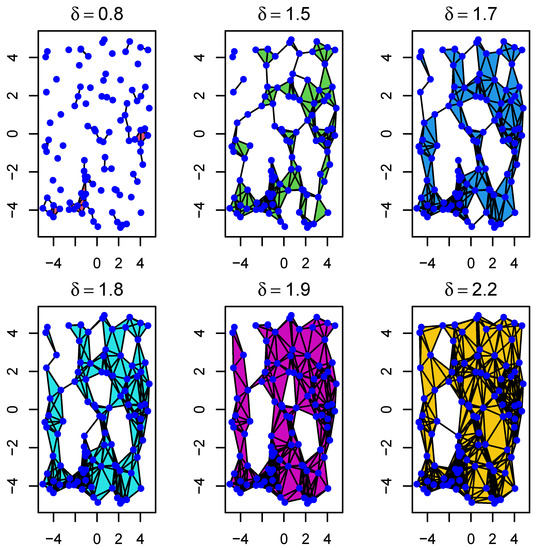
Figure 3. Example of the evolution of Rips complexes $\left\{R_{\delta }\right\}$ through a filtration with parameter $\delta$. As we move from left to right, it shows how sample points (blue dots) first form 0-simplices, then 1-simplices, and so on. In particular, it shows how connected components progressively evolve to form different types of holes.

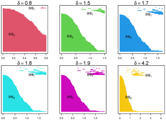
Figure 4. Example of the evolution of barcodes through a filtration with parameter $\delta$ for the same data as above. As we move from left to right, from top to bottom, it shows the appearance and disappearance of lines (${\mathbb{H}}_0$) and holes (${\mathbb{H}}_1$) as the parameter $\delta$ changes. It shows that certain lines and holes persist through the filtration process.

4.2. EEG Epilepsy Data

4.2.1. Data Description

The main purpose of the manuscript is to analyze EEG data. We consider a publicly available (at http://www.meb.unibonn.de/epileptologie/science/physik/eegdata.html, last accessed on 1 June 2023) epilepsy data set. For a thorough description of the data and their cleaning process, see, for instance, [39]. They consist of five sets: A, B, C, D, and E. Each contains 100 single-channel EEG segments of 23.6 s, where A and B represent healthy individuals. Set D represents the data obtained from the epileptogenic zone in patients, and set C represents data obtained from the hippocampus zone. Set E represents the data from seizure prone patients.

4.2.2. Data Analysis

The approach is to first embed the data into a manifold of high dimension. This was already performed in [39]. The dimension $d=12$ was found using the method of false nearest neighbors. Depending on the set used, the size of the data can be very large: for example ($4097\times 100\times 5=2,048,500$), making it very challenging to analyze holistically. In [39], we proposed to construct a complex structure (using all 100 channels for all 5 groups) whose volume changes per group. We would like to analyze the data further from a persistent homology point of view. This would mean analyzing 500 different persistent diagrams and making an inference. We note that simplicial complexes of these data sets are very large (2 Millions+). Fortunately, we can use the Wasserstein distance to compare persistent diagrams. To clarify, we use each of the dimension reduction methods introduced earlier, then proceed with the construction of persistent diagrams. We then compare them by method and by sets (A, B, C, D, and E).

Single-channel Analysis:

Suppose we select at random one channel among the 100 from set D, Figure 5 below represents a three dimensional representation of the embedded data using Takens embedding method (Tak), plotted using the first three delayed coordinates $x=x\left(t\right),y=x(t-\rho ),z=x(t-2\rho )$, where $\rho =1\Delta t$, with $\Delta t=\frac{1}{fs}=5.76$ ms in Figure 5a; then, the first three coordinates in the case of kernel ridge regression (KRR${}_i$) in Figure 5b; ISOMAP (iso.i) in Figure 5c; Laplacian Eigenmaps (LEIM${}_i$) in Figure 5d; fast independent component analysis (ICA${}_i$) in Figure 5e; and t-distributed stochastic neighbor embedding (t-SNE${}_i$) in Figure 5f. From these three dimensional scatter plots, we can visually observe that the t-SNE plot (Figure 5f) is relatively different from the other five since it seems to have more larger voids. How different is difficult to tell with the naked eye. Figure 6 represents their corresponding barcodes. It is much clearer looking at the the persistent diagram for t-SNE (Figure 6f) that it is very different from the other five when looking at ${\mathbb{H}}_0,{\mathbb{H}}_1$, and ${\mathbb{H}}_2$. Now, a visual comparison is not enough to really assert a significant difference. Using the Bottleneck distance, we calculate the distance between the respective persistent diagrams for ${\mathbb{H}}_0$ and ${\mathbb{H}}_1$ in Table 1a and ${\mathbb{H}}_2$ in Table 1b below. We observe from the first table that the Bottleneck distances at ${\mathbb{H}}_0$ and ${\mathbb{H}}_2$ for t-SNE are almost twice as large as for the other methods. They are comparable to that of LEIM at ${\mathbb{H}}_1$. The other methods have comparable Bottleneck distances at ${\mathbb{H}}_0,{\mathbb{H}}_1$, and ${\mathbb{H}}_2$, confirming what we already suspected visually in Figure 5 and Figure 6.

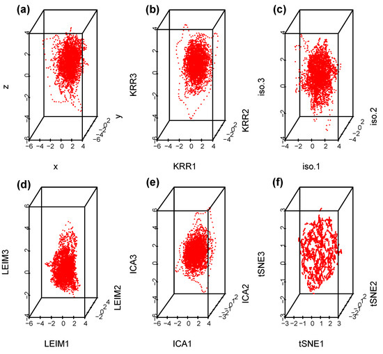
Figure 5. Scatterplots for a Takens projection method (a), KRR method (b), ISOMAP (c), LEIM (d), ICA (e), and t-SNE (f).

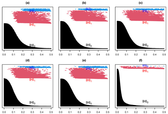
Figure 6. Barcodes for a Takens projection method (a), KRR method (b), ISOMAP (c), LEIM (d), ICA (e), and t-SNE (f).

Table 1. Bottleneck distance between the persistent diagrams above at ${\mathbb{H}}_0$ (a), at ${\mathbb{H}}_1$ and at ${\mathbb{H}}_2$ (b).

(a)
${\mathbb{H}}_0$	Tak	Iso	KRR	ICA	LEIM	TSNE
Tak
Iso	0.0945019
KRR	0.0957546	0.0200035
ICA	0.0982795	0.0157002	0.0071899
LEIM	0.1678820	0.1182656	0.1247918	0.1205499
TSNE	0.2238167	0.1730406	0.1817924	0.1759454	0.1162392
(b)
${\mathbb{H}}_1$/${\mathbb{H}}_2$	Tak	Iso	KRR	ICA	LEIM	TSNE
Tak		0.0363205	0.0301992	0.0292631	0.0291247	0.0551774
Iso	0.0340282		0.0330687	0.0290406	0.0236890	0.0598517
KRR	0.0317261	0.0279460		0.0207599	0.0212138	0.0647935
ICA	0.0310771	0.0270919	0.0208086		0.0242277	0.0611090
LEIM	0.0607389	0.0725585	0.0702695	0.0682761		0.0542615
TSNE	0.0757815	0.0959521	0.0864587	0.0861522	0.0785030

The analysis above was performed using a single channel, selected at random from the set D. It seems to suggest that the t-SNE method is different from the other five dimension reduction methods discussed above. Strictly speaking, non zero Bottleneck distances are an indication of structural topological differences. What they do not say, however, is if the differences observed are significant. To address the issue of significance, we perform a pairwise permutation test. Practically, from set j and channel i, we obtain a persistent diagram ${\mathcal{D}}_i^{\left(j\right)}\sim {\mathcal{P}}^{\left(j\right)}$ where $j\in \left\{1,2,3,4,5\right\},i\in \left\{1,2,\cdots ,15\right\}$, and ${\mathcal{P}}^{\left(j\right)}$ is the true underlying distribution of persistent diagrams; see [40] for the existence of these distributions. We conduct a pairwise permutation test with null hypothesis $H_0:{\mathcal{P}}^{\left(j\right)}={\mathcal{P}}^{\left(j^{\prime }\right)}$ and alternative hypothesis $H_1:{\mathcal{P}}^{\left(j\right)}\ne {\mathcal{P}}^{\left(j^{\prime }\right)}$. We use landscape functions (see [41]) to obtain test statistics. The p.values obtained were found to be very small, suggesting that the differences above are indeed all significant across ${\mathbb{H}}_0,{\mathbb{H}}_1$, and ${\mathbb{H}}_2$.

Multiple-channel Analysis:

(a)

Within set analysis

In each set, we make a random selection of 15 channels, and we compare the Bottleneck distances obtained. This means having 15 tables of distance, such as Table 1b above. There is consistency if the cell value $k(i,j)$ in Table k, where $k\in \left\{1,2,\cdots ,15\right\}$ and $i,j\in \left\{1,2,3,4,5\right\}$, is barely different from $k^{\prime }(i,j)$ of Table $k^{\prime }$. Large differences are an indication of topological differences between the methods within the sets. In Figure 7 below, the y-axis represents Bottleneck distances, and the x-axis represents channels indices. The red color is indicative of the Bottleneck distance between persistent diagrams on ${\mathbb{H}}_1$ and the blue color on ${\mathbb{H}}_2$ from the data generated from each of the methods above. We see that overall, while there are small fluctuations from channels to channels on ${\mathbb{H}}_1$, the largest fluctuations actually occur on ${\mathbb{H}}_2$. A deeper analysis reveals that in fact, the large fluctuations are due to a large distance between t-SNE and the other five methods. This confirms the earlier observations (refer to Figure 6 and Table 1 above) that persistent diagrams are really different on ${\mathbb{H}}_2$. Topologically, this means that shells around cavities or voids that persist are not the same when using different dimension reduction methods. However, the small fluctuations on ${\mathbb{H}}_1$ do not mean that tunnels and holes that persist are the same. Rather, what they do indicate is that they may not be all very different.

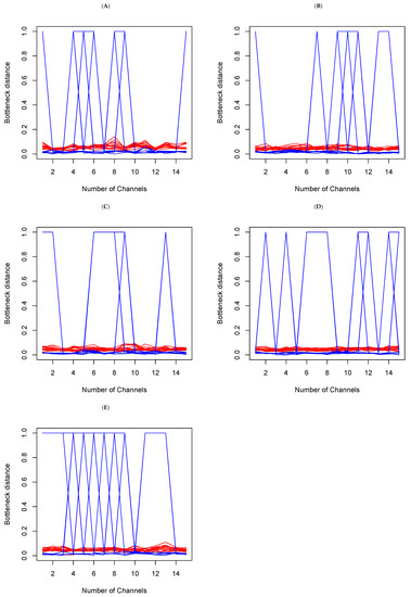
Figure 7. Bottleneck distances between the persistent diagrams for 15 channels within each set (A–E) on ${\mathbb{H}}_1$ and ${\mathbb{H}}_2$ for each of the methods introduced above. The red lines represent the Bottleneck distances between persistent diagrams on ${\mathbb{H}}_1$ and the blue are their counterparts on ${\mathbb{H}}_2$.

(b)

Between set analysis

To analyze the data of the Bottleneck distances between sets, we need summary statistics for each set from the data above. It is clear from Figure 7 that the mean would not be a great summary statistic for ${\mathbb{H}}_1$, as there seem to be too many outliers. We will use the median instead and perform a pairwise Wilcoxon–Mann–Whitney test. Table 2 below shows the p.value on ${\mathbb{H}}_1$ and ${\mathbb{H}}_2$. The take-away is that the last row of the table suggests that set E is statistically topologically different from others on ${\mathbb{H}}_1$, at a significance level of $0.05$. In a way, this is a confirmation of the results obtained in [39] where set E (seizure) was already shown to be statistically different from other sets.

Table 2. P values of Wilcoxon–Mann–Whitney tests between sets of median Bottleneck distances.

${\mathbb{H}}_1$/${\mathbb{H}}_2$	A	B	C	D	E
A		0.1975936	0.3049497	0.2467548	0.7432987
B	0.3202554		0.3835209	0.5066311	0.1707835
C	0.0832231	0.1322987		0.8356690	0.7088614
D	0.2012797	0.6292608	0.6292608		0.5067258
E	0.0049325	0.0157855	0.0157855	0.0114901

5. Concluding Remarks

In this paper, we have revisited the mathematical descriptions of six dimension reduction methods. We have given a brief introduction to the very vast topic of persistent homology. We discussed how to apply persistent homology to the data. In the presence of data (say in three dimensions) obtained either by projecting the data from a high dimension into a smaller dimension (as in Takens) or by performing some sort of dimension reduction, it is not always clear what we see or how different one method is compared to another. From their mathematical description, they seem to represent different objects. Furthermore, obtaining theoretically a clear discrimination procedure between these procedures seems a daunting, if not an outright impossible, task. Topology may offer a solution by looking at persistent artifacts through filtration. From Figure 5, it seems clear that the methods were different, but Figure 6 offers a different perspective. In the end, through the calculation of Bottleneck distances and hypothesis tests, we can safely conclude that the methods are different, topologically speaking, in that the connected components, the tunnels and holes and the shells around cavities or voids, do not match perfectly. Since these methods are indiscriminately used in many applications, the message is that the replication of results from one method to the next may not be guaranteed in the grand scheme of things. It does not, however, render them useless. In fact, our analysis is limited to one data set, meaning that another data set may yield different conclusions. Furthermore, due to the cost in calculation, we were limited to only a handful of samples. Additionally, the Wasserstein distances for $p<\infty$ are extremely costly in time to calculate on a regular computer. Even for $p=\infty$, the Bottleneck distance is also very costly in time to calculate, especially for ${\mathbb{H}}_0$. This explains why, at some point, we did not provide the comparison for ${\mathbb{H}}_0$. Given that some EEG epilepsy data are known to contain some deterministic chaos, it might be worthwhile to study whether persistent homology can also be used for the better understanding of chaotic data in dynamical systems.

References

- Whitney, H. Differentiable manifolds. Ann. Math. 1936, 37, 645–680. [Google Scholar] [CrossRef]
- Takens, F. Detecting strange attractors in turbulence dynamical systems and turbulence. Lect. Notes Math. 1981, 898, 366–381. [Google Scholar]
- Ma, Y.; Fu, Y. Manifold Learning: Theory and Applications; CRC Press: Boca Raton, FL, USA, 2012. [Google Scholar]
- Hotelling, H. Analysis of a complex of statistical variables into principal components. J. Educ. Psychol. 1933, 24, 498–520. [Google Scholar] [CrossRef]
- Ramsay, J.O.; Silverman, B.W. Functional Data Analysis, 2nd ed.; Springer: Berlin/Heidelberg, Germany, 2005. [Google Scholar]
- Cohen, J.; West, S.G.; Aiken, L.S. Applied Multiple Regression/Correlation Analysis for the Behavioral Sciences, 3rd ed.; Lawrence Erlbaum Associates Publishers: Mahwah, NJ, USA, 2003. [Google Scholar]
- Friedman, J.H. Regularized discriminant analysis. J. Am. Stat. Assoc. 1989, 84, 165–175. [Google Scholar] [CrossRef]
- Yu, H.; Yang, J. A direct lda algorithm for high-dimensional data—With application to face recognition. Pattern Recognition 2001, 34, 2067–2069. [Google Scholar] [CrossRef]
- Tenenbaum, J.B.; de Siva, V.; Langford, J.C. A global geometric frameworkfor nonlinear dimensionality reduction. Science 2000, 290, 2319–2323. [Google Scholar] [CrossRef]
- Belkin, M.; Niyogi, P. Laplacian eigenmaps and spectral techniques for embedding and clustering. In Advances in Neural Information Processing Systems 14; Dietterich, T.G., Becker, S., Ghahramani, Z., Eds.; MIT Press: Cambridge, MA, USA, 2002; pp. 585–591. [Google Scholar]
- Hyvärinen, A. Fast and robust fixed-point algorithms for independent component analysis. IEEE Trans. Neural Netw. 1999, 13, 411–430. [Google Scholar] [CrossRef]
- Theodoridis, S. (Ed.) Chapter 11—Learning in reproducing kernel hilbert spaces . In Machine Learning, 2nd ed.; Academic Press: Cambridge, MA, USA, 2020; pp. 531–594. Available online: https://www.sciencedirect.com/science/article/pii/B9780128188033000222 (accessed on 28 June 2023).
- Van der Maaten, L.J.P.; Hinton, G.E. Visualizing data using t-sne. J. Mach. Learn. Res. 2008, 9, 2579–2605. [Google Scholar]
- Naizait, G.; Zhitnikov, A.; Lim, L.-H. Topology of deep neural networks. J. Mach. Learn. Res. 2020, 21, 7503–7542. [Google Scholar]
- Chan, J.M.; Carlsson, G.; Rabadan, R. Topology of viral evolution. Proc. Natl. Acad. Sci. USA 2013, 110, 18566–18571. [Google Scholar] [CrossRef]
- Otter, N.; Porter, M.A.; Tillman, U.; Grindrod, P.; Harrington, H.A. A roadmap for the computationof persistent homology. EPJ Data Sci. 2017, 6, 17. [Google Scholar] [CrossRef]
- De Silva, V.G.; Ghrist, R. Coverage in sensor networks via persistent homology. Algebr. Geom. Topol. 2007, 7, 339–358. [Google Scholar] [CrossRef]
- Gameiro, M.; Hiraoka, Y.; Izumi, S.; Mischaikow, K.M.K.; Nanda, K. A topological measurement of proteincompressibility. Jpn. J. Ind. Appl. Math. 2015, 32, 1–17. [Google Scholar] [CrossRef]
- Xia, K.; Wei, G.-W. Persistent homology analysis of protein structure, flexibility, and folding. Int. J. Numer. Methods Biomed. Eng. 2014, 30, 814–844. [Google Scholar] [CrossRef] [PubMed]
- Emmett, K.; Schweinhart, N.; Rabadán, R. Multiscale topology of chromatin folding. In Proceedings of the 9th EAIinternational Conference on Bio-Inspired Information and Communications Technologies, BICT’15, ICST 2016, New York City, NY, USA, 3–5 December 2015; pp. 177–180. [Google Scholar]
- Rizvi, A.; Camara, P.; Kandror, E.; Roberts, T.; Schieren, I.; Maniatis, T.; Rabadán, R. Single-cell topological rna-seqanalysis reveals insights into cellular differentiation and development. Nat. Biotechnol. 2017, 35, 551–560. [Google Scholar] [CrossRef] [PubMed]
- Bhattacharya, S.; Ghrist, R.; Kumar, V. Persistent homology for path planning in uncertain environments. IEEE Trans. Robot. 2015, 31, 578–590. [Google Scholar] [CrossRef]
- Pokorny, F.T.; Hawasly, M.; Ramamoorthy, S. Topological trajectory classification with filtrations of simplicialcomplexes and persistent homology. Int. J. Robot. Res. 2016, 35, 204–223. [Google Scholar] [CrossRef]
- Vasudevan, R.; Ames, A.; Bajcsy, R. Persistent homology for automatic determination of human-data based costof bipedal walking. Nonlinear Anal. Hybrid Syst. 2013, 7, 101–115. [Google Scholar] [CrossRef]
- Chung, M.K.; Bubenik, P.; Kim, P.T. Persistence diagrams of cortical surface data. In Information Processing in Medical Imaging. Lecture Notes in Computer Science; Prince, J.L., Pham, D.L., Myers, K.J., Eds.; Springer: Berlin, Germany, 2009; Volume 5636, pp. 386–397. [Google Scholar]
- Guillemard, M.; Boche, H.; Kutyniok, G.; Philipp, F. Persistence diagrams of cortical surface data. In Proceedings of the 10th International Conference on Sampling Theory and Applications, Bremen, Germany, 1–5 July 2013; pp. 309–312. [Google Scholar]
- Taylor, D.; Klimm, F.; Harrington, H.A.; Kramár, M.; Mischaikow, K.; Porter, M.A.; Mucha, P.J. Topological data analysis ofcontagion maps for examining spreading processes on networks. Nat. Commun. 2015, 6, 7723. [Google Scholar] [CrossRef]
- Leibon, G.; Pauls, S.; Rockmore, D.; Savell, R. Topological structures in the equities market network. Proc. Natl. Acad. Sci. USA 2008, 105, 20589–20594. [Google Scholar] [CrossRef]
- Giusti, C.; Ghrist, R.; Bassett, D. Two’s company and three (or more) is a simplex. J. Comput. Neurosci. 2016, 41, 1–14. [Google Scholar] [CrossRef] [PubMed]
- Sizemore, A.E.; Phillips-Cremins, J.E.; Ghrist, R.; Bassett, D.S. The importance of the whole: Topological data analysis for the network neuroscientist. Netw. Neurosci. 2019, 3, 656–673. [Google Scholar] [CrossRef]
- Maletić, S.; Zhao, Y.; Rajković, M. Persistent topological features of dynamical systems. Chaos 2016, 26, 053105. [Google Scholar] [CrossRef] [PubMed]
- Chung, M.K.; Ramos, C.G.; Paiva, J.; Mathis, F.B.; Prabharakaren, V.; Nair, V.A.; Meyerand, E.; Hermann, B.P.; Binder, J.R.; Struck, A.F. Unified topological inference for brainnetworks in temporal lobe epilepsy using thewasserstein distance. arXiv 2023, arXiv:2302.06673. [Google Scholar]
- Torgerson, W.S. Multidimensional scaling: I. theory and method. Psychometrika 1952, 17, 410–419. [Google Scholar] [CrossRef]
- Jäntschi, L. Multiple linear regressions by maximizing the likelihood under assumption of generalized gauss-laplace distribution of the error. Comput. Math. Methods Med. 2016, 2016, 8578156. [Google Scholar] [CrossRef] [PubMed]
- Jäntschi, L. Symmetry in regression analysis: Perpendicular offsets—The case of a photovoltaic cell. Symmetry 2023, 15, 948. [Google Scholar] [CrossRef]
- NSilver, The Signal and Noise: Why So Many Predictions Fail—But Some Dont; The Penguin Press: London, UK, 2012.
- Hinton, G.E.; Roweis, S. Stochastic neighbor embedding. In Advances in Neural Information Processing Systems; Becker, S., Thrun, S., Obermayer, K., Eds.; MIT Press: Cambridge, MA, USA, 2002; Volume 15. [Google Scholar]
- Ghrist, R. Barcodes: The persistent topology of data. Bull. Amer. Math. Soc. 2008, 45, 61–75. [Google Scholar] [CrossRef]
- Kwessi, E.; Edwards, L. Analysis of eeg time series data using complex structurization. Neural Comput. 2021, 33, 1942–1969. [Google Scholar] [CrossRef]
- Mileyko, Y.; Mukherjee, S.; Harer, J. Probability measures on the space of persistence diagrams. Inverse Probl. 2011, 27, 124007. [Google Scholar] [CrossRef]
- Berry, E.; Chen, Y.-C.; Cisewski-Kehe, J.; Fasy, B.T. Functional summaries of persistence diagrams. J. Appl. Comput. Topol. 2020, 4, 211–262. [Google Scholar] [CrossRef]
Disclaimer/Publisher’s Note: The statements, opinions and data contained in all publications are solely those of the individual author(s) and contributor(s) and not of MDPI and/or the editor(s). MDPI and/or the editor(s) disclaim responsibility for any injury to people or property resulting from any ideas, methods, instructions or products referred to in the content. |
© 2023 by the author. Licensee MDPI, Basel, Switzerland. This article is an open access article distributed under the terms and conditions of the Creative Commons Attribution (CC BY) license (https://creativecommons.org/licenses/by/4.0/).