Analysis of WE Parameters of Life Using Adaptive-Progressively Type-II Hybrid Censored Mechanical Equipment Data

Abstract

A new two-parameter weighted-exponential (WE) distribution, as a beneficial competitor model to other lifetime distributions, namely: generalized exponential, gamma, and Weibull distributions, is studied in the presence of adaptive progressive Type-II hybrid data. Thus, based on different frequentist and Bayesian estimation methods, we study the inferential problem of the WE parameters as well as related reliability indices, including survival and failure functions. In frequentist setups, besides the standard likelihood-based estimation, the product of spacing (PS) approach is also taken into account for estimating all unknown parameters of life. Making use of the delta method and the observed Fisher information of the frequentist estimators, approximated asymptotic confidence intervals for all unknown parameters are acquired. In Bayes methodology, from the squared-error loss with independent gamma density priors, the point and interval estimates of the unknown parameters are offered using both joint likelihood and the product of spacings functions. Because a closed solution to the Bayes estimators is not accessible, the Metropolis–Hastings sampler is presented to approximate the Bayes estimates and also to create their associated highest interval posterior density estimates. To figure out the effectiveness of the developed approaches, extensive Monte Carlo experiments are implemented. To highlight the applicability of the offered methodologies in practice, one real-life data set consisting of 30 failure times of repairable mechanical equipment is analyzed. This application demonstrated that the offered WE model provides a better fit compared to the other eight lifetime models.

1. Introduction

Censoring is a popular technique in reliability and life testing investigations. The experimenter must have prior expertise with various test conditions, including time, cost, or money limits, when unit removal is scheduled in advance prior to failure. In reliability investigations, the most commonly employed censoring techniques are time censoring (Type-I) and failure censoring (Type-II). One of these techniques’ primary flaws is that things cannot be removed from the experiment at any point other than the end, so progressive Type-II (T2P) censoring is suggested; for further details, see Balakrishnan and Cramer [1]. Although the Type-I progressively hybrid censoring, proposed by Kundu and Joarder [2], ensures that the experiment stops at a predetermined time, the effective sample size collected may be too small; thus, the estimation approach cannot be effective. For this reason, Ng et al. [3] suggested adaptive progressive Type-II hybrid (T2APH) censoring. This life test plan has become widely common in survival studies and is conducted as follows: Suppose n (size of total independent identical items), $m(<n)$ (size of failed subjects), $\underline{\mathbf{R}}=(R_1,R_2,\cdots ,R_m)$ (T2P censoring), $T\in (0,\infty )$ (threshold time), are preassigned. This mechanism allows $R_i,i=1,2,\cdots ,m$ to change accordingly during the examination and confers the experiment time to run over T. If $Y_{m:m:n}<T$, just like the conventional T2P strategy, end the test at $Y_{m:m:n}$. Otherwise, if $Y_{d:m:n}<T<Y_{d+1:m:n}$, where $d(=1,2,\cdots ,m-1)$ denotes the total number of failures up to T, the practitioner must stop the removal items beyond T, i.e., $R_i=0$ for $i=d+1,\cdots ,m-1$ and end the test at $Y_{m:m:n}$. However, the number of staying live units (say $R_m^{*}$) when $Y_{m:m:n}<T$ and $Y_{d:m:n}<T$ are $R_m^{*}=n-m-{\sum }_{i=1}^{m-1}{R}_i$ and $R_m^{*}=n-m-{\sum }_{i=1}^d{R}_i$, respectively.

Let $\underline{\mathbf{y}}=\left\{(Y_{1:m:n},R_1),\cdots ,(Y_{d:m:n},R_d),(Y_{d+1m:n},0),\cdots ,(Y_{m-1:m:n},0),(Y_{m:m:n},R_m)\right\}$ be a T2APH sample is obtained from a population having a cumulative distribution function (CDF) $F(·)$ and probability density function (PDF) $f(·)$, then the joint likelihood function (LF) of T2APH, where $\Omega$ refers to the vector of parameters under interest, is

$$L\left(\left.\Omega \right|\underline{\mathbf{y}}\right)=A_d{\prod }_{i=1}^{m}f\left(y_{i:m:n};\Omega \right){\prod }_{i=1}^d{\left[\overline{F}(y_{i:m:n};\Omega )\right]}^{R_i}{\left[\overline{F}(y_{m:m:n};\Omega )\right]}^{R_m^{*}},$$

(1)

where $A_d$ is a constant and $\overline{F}(·)=1-F(·)$. It should be noted that this proposed strategy ensures that the life test ends when the required effective sample size is reached; see, for example, Elshahhat and Nassar [4,5].

Besides (1), the PS methodology is also inserted as a good competitive approach to the conventional likelihood. The PS method was independently investigated by Cheng and Amin [6] and Ranneby [7]. Similar to the logic of obtaining the MLEs, maximum product spacing estimators (PSEs) can be obtained by maximizing the PS function. For skewed distributions, Anatolyev and Kosenok [8] demonstrated that the PSEs are more efficient than the traditional MLEs. Following El-Sherpieny et al. [9], the T2APH using maximum PS method, $S(·)$, can be defined as

$$S\left(\left.\Omega \right|\underline{\mathbf{y}}\right)=B_d\prod _{i=1}^{m+1}\left[F\left(y_{i:m:n};\Omega \right)-F\left(y_{i-1:m:n};\Omega \right)\right]\prod _{i=1}^d{\left[\overline{F}(y_{i:m:n};\Omega )\right]}^{R_i}{\left[\overline{F}(y_{m:m:n};\Omega )\right]}^{R_m^{*}},$$

(2)

where $B_d$ is a constant, $F\left(y_{0:m:n};\Omega \right)\equiv 0$ and $F\left(y_{m+1:m:n};\Omega \right)\equiv 1$.

The two-parameter weighted-exponential (WE) distribution was suggested by Gupta and Kundu [10] by adding a new skewness parameter to the traditional exponential distribution. They also stated that the WE density shape is quite obvious compared to the other extended exponential lifetime models, including: gamma, Weibull, and generalized exponential distributions. Moreover, in many practical situations, the WE distribution has superior properties and may be utilized to fit lifetime data compared to other models in the statistical literature. Thus, the WE distribution might be a good alternate choice to analyze skewed-data. Further, Dey et al. [11] proposed several properties and derived various estimators of the WE parameters under complete sampling. However, suppose Y is a random life variable of an item that follows $WE\left(\rho \right)$, where $\rho ={(\gamma ,\sigma )}^{\mathsf{T}}$. Hence, the respective PDF and CDF of Y are

$$f(y;\rho )={\sigma }^{-1}(\sigma +1)\gamma e^{-\gamma y}\left(1-e^{-\sigma \gamma y}\right),y>0,$$

(3)

and

$$F(y;\rho )=1-{\sigma }^{-1}{e}^{-\gamma y}\left(1+\sigma -e^{-\sigma \gamma y}\right),$$

(4)

where $\gamma >0$ and $\sigma >0$ denote the scale and shape parameters, respectively. Consequently, the reliability function (RF) (say $R(·)$) and hazard rate function (HRF) (say $h(·)$) of the WE model, at time $t>0$, are given by

$$R(t;\rho )={\sigma }^{-1}{e}^{-\gamma t}\left(1+\sigma -e^{-\sigma \gamma t}\right),t>0,$$

(5)

and

$$h(t;\rho )=\gamma \left(\sigma +1\right)\frac{1-e^{-\sigma \gamma t}}{1+\sigma -e^{-\sigma \gamma t}},$$

(6)

respectively. Setting $\gamma =1$ in (4), two sub-models can be obtained as special cases, namely:

• Gamma distribution with shape parameter 2 when $\sigma \to 0$.
• Generalized-exponential distribution with shape parameter 2 when $\sigma =1$.

Using some specified values in the range of the parameters $\sigma$ and $\gamma$, different shapes of the density and failure rate functions of the WE distribution are shown in Figure 1. It shows that the density shapes of the WE distribution are always log-concave and unimodal with the mode at $ln(\sigma +1)/\sigma$; in addition, the HRF has a monotone increasing function for all nonnegative values of $\sigma$ and $\gamma$ (see Gupta and Kundu [10]). Several works in the recent decade have explored the inference problem of the WE parameters; for example, Farahani and Khorram [12] examined the Bayesian inference for WE distribution parameters under Type-II censoring, and Tian and Gui [13] discussed the WE parameters in the presence of T2P-competing risks data.

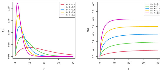
Figure 1. Plots of the density and hazard rate functions of the WE distribution.

To the best of our knowledge of T2APH data, we are not aware of any work related to inferring the WE parameters $\sigma$ and $\gamma$ and/or the reliability $R\left(t\right)$ and $h\left(t\right)$ functions. As a result, to bridge this gap, the objectives of the current study are fourfold:

• Develop both point and interval estimates of $\sigma$, $\gamma$, $R\left(t\right)$ and $h\left(t\right)$ using T2APH samples by exclusively focusing on both frequentist and Bayesian inferential methods.
• Acquire the maximum likelihood and product of spacings estimates of $\sigma$, $\gamma$, $R\left(t\right)$ and $h\left(t\right)$. Create the approximate confidence interval (ACI) bounds of the unknown quantities using the observed Fisher information obtained from both the LF and PS approaches.
• Explore the PS method as an alternative to the traditional LF method and investigate both in two Bayesian estimation setups for unknown parameters, reliability function, and hazard function. Use independent gamma density priors against the squared-error loss to develop the Bayes estimates. Approximate the Bayes estimates and their credible intervals via Markov-chain Monte-Carlo (MCMC) techniques.
• Compare the effectiveness of the offered approaches based on several accuracy criteria, namely: simulated bias, mean squared error, and length of confidence interval values via Monte Carlo simulations. Illustrate a mechanical data set to discuss the suggested methodologies and to highlight the WE distribution’s superiority and flexibility over other eight lifetime models in the literature, namely: Weibull, gamma, Nadarajah–Haghighi, weighted Nadarajah–Haghighi, alpha power exponential, Weibull-exponential, generalized gamma, and generalized beta distributions.

The remainder of the paper is structured as follows: Section 2 provides the frequentist estimates. In Section 3, Bayesian (point/interval) estimations are developed. Section 4 presents the simulated outcomes. Real data results are highlighted in Section 5. Finally, Section 6 presents the conclusions and recommendations of the study.

2. Frequentist Estimations

Here, we shall consider both LF and PS techniques to derive point as well as interval estimators of $\sigma$, $\gamma$, $R\left(t\right)$, and $h\left(t\right)$. For simplicity in notation, the symbol $y_{i:m:n}$ is used as $y_i$. Assume that $Y_1<\cdots <Y_d<T<Y_{d+1}<\cdots <Y_m$ with $(R_1,\cdots ,R_d,0,\cdots ,0,$$n-{\sum }_{i=1}^d{R}_i-m)$ is a T2APH sample of size m from $\mathrm{WE}(\sigma ,\gamma )$.

2.1. Likelihood Estimators

Taking (4) and (3) into (1), we can express the proportionality likelihood (1) function as

$$L\left(\left.\sigma ,\gamma \right|\underline{\mathbf{y}}\right)\propto \frac{{\left(\sigma +1\right)}^m}{{\sigma }^n}{\gamma }^m{e}^{-\gamma {\psi }_1\left(\underline{\mathbf{y}}\right)}{\left(\xi \left(y_m;\sigma ,\gamma \right)\right)}^{R_m^{*}}\prod _{i=1}^d{\left(\xi \left(y_i;\sigma ,\gamma \right)\right)}^{R_i}\prod _{i=1}^m\left(1-exp\left(-\sigma \gamma y_i\right)\right),$$

(7)

where ${\psi }_1\left(\underline{\mathbf{y}}\right)={\sum }_{i=1}^m{y}_i+{\sum }_{i=1}^d{y}_i{R}_i+y_m{R}_m^{*}$, $\xi \left(y_m;\sigma ,\gamma \right)=1+\sigma -exp\left(-\sigma \gamma y_m\right)$ and $\xi \left(y_i;\sigma ,\gamma \right)=1+\sigma -exp\left(-\sigma \gamma y_i\right)$.

The log-likelihood (say $\ell (·)=logL(·)$) function of (7) becomes

$$\begin{array}{cc}\hfill \ell \left(\left.\sigma ,\gamma \right|\underline{\mathbf{y}}\right)& =mlog\left(\gamma \left(\sigma +1\right)\right)-nlog\left(\sigma \right)-\gamma {\psi }_1\left(\underline{\mathbf{y}}\right)+R_m^{*}log\left(\xi \left(y_m;\sigma ,\gamma \right)\right)\hfill \\ \hfill & +{\sum }_{i=1}^d{R}_{i}log\left(\xi \left(y_i;\sigma ,\gamma \right)\right)+{\sum }_{i=1}^{m}log\left(1-exp\left(-\sigma \gamma y_i\right)\right).\hfill \end{array}$$

(8)

Differentiating (8) partially with regard to $\sigma$ and $\gamma$ as

$$\frac{\partial \ell }{\partial \sigma }=\frac{m}{\sigma +1}-\frac{n}{\sigma }+R_m^{*}\frac{{\xi }_{\sigma }^{\prime }\left(y_m;\sigma ,\gamma \right)}{\xi \left(y_m;\sigma ,\gamma \right)}+{\sum }_{i=1}^d{R}_i\frac{{\xi }_{\sigma }^{\prime }\left(y_i;\sigma ,\gamma \right)}{\xi \left(y_i;\sigma ,\gamma \right)}+\gamma {\sum }_{i=1}^m\frac{y_{i}exp\left(-\sigma \gamma y_i\right)}{\left(1-exp\left(-\sigma \gamma y_i\right)\right)},$$

(9)

and

$$\frac{\partial \ell }{\partial \gamma }=\frac{m}{\gamma }-{\psi }_1\left(\underline{\mathbf{y}}\right)+R_m^{*}\frac{{\xi }_{\gamma }^{\prime }\left(y_m;\sigma ,\gamma \right)}{\xi \left(y_m;\sigma ,\gamma \right)}+{\sum }_{i=1}^d{R}_i\frac{{\xi }_{\gamma }^{\prime }\left(y_i;\sigma ,\gamma \right)}{\xi \left(y_i;\sigma ,\gamma \right)}+\sigma {\sum }_{i=1}^m\frac{y_{i}exp\left(-\sigma \gamma y_i\right)}{\left(1-exp\left(-\sigma \gamma y_i\right)\right)},$$

(10)

respectively, where ${\xi }_{\sigma }^{\prime }\left(y_m;\sigma ,\gamma \right)=1+\gamma y_{m}exp\left(-\sigma \gamma y_m\right)$, ${\xi }_{\gamma }^{\prime }\left(y_m;\sigma ,\gamma \right)=\sigma y_{m}exp\left(-\sigma \gamma y_m\right)$, ${\xi }_{\sigma }^{\prime }\left(y_i;\sigma ,\gamma \right)=1+\gamma y_{i}exp\left(-\sigma \gamma y_i\right)$ and ${\xi }_{\gamma }^{\prime }\left(y_i;\sigma ,\gamma \right)=\sigma y_{i}exp\left(-\sigma \gamma y_i\right)$ for $i=1,\cdots ,d$.

Analytical closed-solutions from (9) and (10) for the MLEs $\widehat{\sigma }$ and $\widehat{\gamma }$ of $\sigma$ and $\gamma$, respectively, are not available. Thus, the Newton–Raphson (NR) technique via ‘$\mathsf{maxLik}$’ package (by Henningsen and Toomet [14]) may be implemented to evaluate the acquired $\widehat{\sigma }$ and $\widehat{\gamma }$ estimators. Once those are calculated, using (5) and (6), the MLEs $\widehat{R}\left(t\right)$ and $\widehat{h}\left(t\right)$ of $R\left(t\right)$ and $h\left(t\right)$ at time $t>0$ can be offered directly as

$$\widehat{R}\left(t\right)={\widehat{\sigma }}^{-1}{e}^{-\widehat{\gamma }t}\left(1+\widehat{\sigma }-e^{-\widehat{\sigma }\widehat{\gamma }t}\right),t>0,\mathrm{and}\widehat{h}\left(t\right)=\widehat{\gamma }\left(\widehat{\sigma }+1\right)\frac{1-e^{-\widehat{\sigma }\widehat{\gamma }t}}{1+\widehat{\sigma }-e^{-\widehat{\sigma }\widehat{\gamma }t}},t>0.$$

2.2. Product of Spacings Estimators

Taking (4) and (3) into (2), the product of spacings (2) function becomes

$$S\left(\left.\sigma ,\gamma \right|\underline{\mathbf{y}}\right)\propto \frac{e^{-\gamma {\psi }_2\left(\underline{\mathbf{y}}\right)}}{{\sigma }^{n+1}}\prod _{i=1}^{m+1}\left[\zeta \left(y_{i-1};\sigma ,\gamma \right)-\zeta \left(y_i;\sigma ,\gamma \right)\right]\prod _{i=1}^d{\left(\xi \left(y_i;\sigma ,\gamma \right)\right)}^{R_i}{\left(\xi \left(y_m;\sigma ,\gamma \right)\right)}^{R_m^{*}},$$

(11)

where ${\psi }_2\left(\underline{\mathbf{y}}\right)={\sum }_{i=1}^d{y}_i{R}_i+y_m{R}_m^{*}$ and $\zeta \left(y_i;\sigma ,\gamma \right)=e^{-\gamma y_i}\left(1+\sigma -e^{-\sigma \gamma y_i}\right)$.

From (11), the PSEs $\widehat{\sigma }$ and $\widehat{\gamma }$ of $\sigma$ and $\gamma$, respectively, can be directly acquired by maximizing the log-PS (say $s(·)\propto logS(·)$) function as

$$\begin{array}{cc}\hfill s\left(\left.\sigma ,\gamma \right|\underline{\mathbf{y}}\right)& \propto -\gamma {\psi }_2\left(\underline{\mathbf{y}}\right)-\left(n+1\right)log\left(\sigma \right)+R_m^{*}log\left(\xi \left(y_m;\sigma ,\gamma \right)\right)\hfill \\ \hfill & +{\sum }_{i=1}^d{R}_{i}log\left(\xi \left(y_i;\sigma ,\gamma \right)\right)+{\sum }_{i=1}^{m}log\left[\zeta \left(y_{i-1};\sigma ,\gamma \right)-\zeta \left(y_i;\sigma ,\gamma \right)\right].\hfill \end{array}$$

(12)

Making partially differentiated of (12) in respect of $\sigma$ and $\gamma$, we have two nonlinear expressions that must be calculated simultaneously to acquire both $\widehat{\sigma }$ and $\widehat{\gamma }$ as

$$\frac{\partial s}{\partial \sigma }=-\frac{\left(n+1\right)}{\sigma }+R_m^{*}\frac{{\xi }_{\sigma }^{\prime }\left(y_m;\sigma ,\gamma \right)}{\xi \left(y_m;\sigma ,\gamma \right)}+\sum _{i=1}^d{R}_i\frac{{\xi }_{\sigma }^{\prime }\left(y_i;\sigma ,\gamma \right)}{\xi \left(y_i;\sigma ,\gamma \right)}+\sum _{i=1}^{m+1}\left[\frac{{\zeta }_{\sigma }^{\prime }\left(y_{i-1};\sigma ,\gamma \right)-{\zeta }_{\sigma }^{\prime }\left(y_i;\sigma ,\gamma \right)}{\zeta \left(y_{i-1};\sigma ,\gamma \right)-\zeta \left(y_i;\sigma ,\gamma \right)}\right],$$

(13)

and

$$\frac{\partial s}{\partial \gamma }=-{\psi }_2\left(\underline{\mathbf{y}}\right)+R_m^{*}\frac{{\xi }_{\gamma }^{\prime }\left(y_m;\sigma ,\gamma \right)}{\xi \left(y_m;\sigma ,\gamma \right)}+\sum _{i=1}^d{R}_i\frac{{\xi }_{\gamma }^{\prime }\left(y_i;\sigma ,\gamma \right)}{\xi \left(y_i;\sigma ,\gamma \right)}+\sum _{i=1}^{m+1}\left[\frac{{\zeta }_{\gamma }^{\prime }\left(y_{i-1};\sigma ,\gamma \right)-{\zeta }_{\gamma }^{\prime }\left(y_i;\sigma ,\gamma \right)}{\zeta \left(y_{i-1};\sigma ,\gamma \right)-\zeta \left(y_i;\sigma ,\gamma \right)}\right],$$

(14)

respectively, where ${\zeta }_{\sigma }^{\prime }\left(y_i;\sigma ,\gamma \right)=e^{-\gamma y_i}{\xi }_{\sigma }^{\prime }\left(y_i;\sigma ,\gamma \right)$ and ${\zeta }_{\gamma }^{\prime }\left(y_i;\sigma ,\gamma \right)=e^{-\gamma y_i}\left[{\xi }_{\gamma }^{\prime }\left(y_i;\sigma ,\gamma \right)-y_i\xi \left(y_i;\sigma ,\gamma \right)\right]$.

As in the MLEs $\widehat{\sigma }$ and $\widehat{\gamma }$, there is no closed solution for the PSEs $\widehat{\sigma }$ and $\widehat{\gamma }$. Again, we recommend utilizing the NR method to obtain the PSEs $\widehat{\sigma }$ and $\widehat{\gamma }$ from (13) and (14), respectively. Following Cheng and Amin [6], we can point out that the offered PSEs $\widehat{\sigma }$ and $\widehat{\gamma }$ have the same characteristics as in the case of $\widehat{\sigma }$ and $\widehat{\gamma }$. Thus, the PSEs $\widehat{R}\left(t\right)$ and $\widehat{h}\left(t\right)$ of $R\left(t\right)$ and $h\left(t\right)$ can be easily acquired, respectively, as

$$\widehat{R}\left(t\right)={\widehat{\sigma }}^{-1}{e}^{-\widehat{\gamma }t}\left(1+\widehat{\sigma }-e^{-\widehat{\sigma }\widehat{\gamma }t}\right),t>0,$$

and

$$\widehat{h}\left(t\right)=\widehat{\gamma }(\widehat{\sigma }+1)\frac{1-e^{-\widehat{\sigma }\widehat{\gamma }t}}{1+\widehat{\sigma }-e^{-\widehat{\sigma }\widehat{\gamma }t}},t>0.$$

2.3. Asymptotic Intervals

Here, we construct the $100(1-\nu )\%$ ACI of $\sigma$, $\gamma$, $R\left(t\right)$ or $h\left(t\right)$, say $\omega =(\sigma ,\gamma ,R(t),h(t\left)\right)$; the Fisher’s information matrix ${\mathbf{I}}_{ij}(\Omega )=E\left[-\left({\partial }^2\ell \left(\left.\Omega \right|\underline{\mathbf{y}}\right)\right)/\partial {\Omega }^2\right],i,j=1,2$. Since the Fisher ${\mathbf{I}}_{ij},i,j=1,2$ members cannot be expressed in closed formulas, both variances and covariances (V-C) matrix of the MLEs $\widehat{\sigma }$ and $\widehat{\gamma }$ can be offered by inverting $\mathbf{I}(\Omega )$ with ignoring E and changing ($\sigma ,\gamma$) with their ($\widehat{\sigma },\widehat{\gamma }$)—see Lawless [15]. However, from (8), the approximate V-C matrix ${\mathbf{I}}^{-1}(\widehat{\sigma },\widehat{\gamma })$ of the acquired MLEs $\widehat{\sigma }$ and $\widehat{\gamma }$ is given by

$${\mathbf{I}}^{-1}(\widehat{\sigma },\widehat{\gamma })={\left[\begin{array}{cc}-{\ell }_{11}& -{\ell }_{12}\\ -{\ell }_{21}& -{\ell }_{22}\end{array}\right]}_{(\widehat{\sigma },\widehat{\gamma })}^{-1}=\left[\begin{array}{cc}{\widehat{\upsilon }}_{\widehat{\sigma }\widehat{\sigma }}& {\widehat{\upsilon }}_{\widehat{\sigma }\widehat{\gamma }}\\ {\widehat{\upsilon }}_{\widehat{\gamma }\widehat{\sigma }}& {\widehat{\upsilon }}_{\widehat{\gamma }\widehat{\gamma }}\end{array}\right].$$

(15)

Similarly, from (12), the approximate V-C matrix ${\mathbf{I}}^{-1}(\widehat{\sigma },\widehat{\gamma })$ of the acquired PSEs $\widehat{\sigma }$ and $\widehat{\gamma }$ is given by

$${\mathbf{I}}^{-1}(\widehat{\sigma },\widehat{\gamma })={\left[\begin{array}{cc}-s_{11}& -s_{12}\\ -s_{21}& -s_{22}\end{array}\right]}_{(\widehat{\sigma },\widehat{\gamma })}^{-1}=\left[\begin{array}{cc}{\widehat{\upsilon }}_{\widehat{\sigma }\widehat{\sigma }}& {\widehat{\upsilon }}_{\widehat{\sigma }\widehat{\gamma }}\\ {\widehat{\upsilon }}_{\widehat{\gamma }\widehat{\sigma }}& {\widehat{\upsilon }}_{\widehat{\gamma }\widehat{\gamma }}\end{array}\right].$$

(16)

In Appendix A and Appendix B, the items ${\ell }_{ij}$ and $s_{ij}$ for $i,j=1,2$ are presented, respectively. Then, the respective $100(1-\nu )\%$ two-sided ACIs of $\sigma$ and $\gamma$ are given by

$$\widehat{\sigma }\mp z_{\nu /2}\sqrt{{\widehat{\upsilon }}_{\widehat{\sigma }\widehat{\sigma }}}\mathrm{and}\widehat{\gamma }\mp z_{\nu /2}\sqrt{{\widehat{\upsilon }}_{\widehat{\gamma }\widehat{\gamma }}},$$

where $z_{\nu /2}$ is the quantile values of a standard normal distribution.

Now, following Greene [16], we shall use the delta technique in turn to estimate the approximated variances of $R\left(t\right)$ and $h\left(t\right)$, respectively, as

$${\widehat{\upsilon }}_R=\left[{\Lambda }_R{\mathbf{I}}^{-1}(\sigma ,\gamma ){\Lambda }_R^{\mathbf{T}}\right]{|}_{(\widehat{\sigma },\widehat{\gamma })},\mathrm{and}{\widehat{\upsilon }}_h=\left[{\Lambda }_{h\left(t\right)}{\mathbf{I}}^{-1}(\sigma ,\gamma ){\Lambda }_h^{\mathbf{T}}\right]{|}_{(\widehat{\sigma },\widehat{\gamma })},$$

where ${\Lambda }_R$ and ${\Lambda }_h$ are the gradient of $R\left(t\right)$ and $h\left(t\right)$ obtained at $\widehat{\sigma }$ and $\widehat{\gamma }$, as

$${\Lambda }_R=\left[\frac{\partial R\left(t\right)}{\partial \sigma },\frac{\partial R\left(t\right)}{\partial \gamma }\right]\mathrm{and}{\Lambda }_h=\left[\frac{\partial h\left(t\right)}{\partial \sigma },\frac{\partial h\left(t\right)}{\partial \gamma }\right],$$

respectively.

Thus, the $100(1-\nu )\%$ two-sided ACIs of $R\left(t\right)$ and $h\left(t\right)$, using their MLEs $\widehat{R}\left(t\right)$ and $\widehat{h}\left(t\right)$, are given by

$$\widehat{R}\left(t\right)\mp z_{\nu /2}\sqrt{{\widehat{\upsilon }}_R}\mathrm{and}\widehat{h}\left(t\right)\mp z_{\nu /2}\sqrt{{\widehat{\upsilon }}_h},$$

respectively. In an identical manner, from (16), the $100(1-\nu )\%$ ACIs of $\sigma$, $\gamma$, $R\left(t\right)$, and $h\left(t\right)$ using their PSEs $\widehat{\sigma }$, $\widehat{\gamma }$, $\widehat{R}\left(t\right)$ and $\widehat{h}\left(t\right)$, respectively, can be easily created.

3. Bayes Estimations

This section considers the Bayes estimates of $\sigma$, $\gamma$, $R\left(t\right)$, and $h\left(t\right)$ in addition to the associated HPD intervals.

3.1. Prior and Loss Functions

It is well known that the gamma prior based on its hyperparameter values has a wide variety of shapes; thus, applying independent gamma priors is thus a relatively simple method that may yield discoveries with more explicit posterior density representations. Thus, the WE parameters $\sigma$ and $\gamma$ are considered to follow $Gamma({\alpha }_1,{\beta }_1)$ and $Gamma({\alpha }_2,{\beta }_2)$, respectively. The joint prior PDF of $\sigma$ and $\gamma$, where the hyperparameters ${\alpha }_i,{\beta }_i>0,i=1,2,$ are selected to represent past information, becomes

$$\pi \left(\sigma ,\gamma \right)\propto {\sigma }^{{\alpha }_1-1}{\gamma }^{{\alpha }_2-1}{e}^{-\left({\beta }_1\sigma +{\beta }_2\gamma \right)},\sigma ,\gamma >0.$$

(17)

In Bayesian methodology, determining symmetric (or asymmetric) loss is an important issue. Thus, the SEL function (which is the most often utilized symmetric loss), say $\mathcal{L}(·)$, is

$$\mathcal{L}\left(\mu ,\tilde{\mu }\right)={\left(\tilde{\mu }-\mu \right)}^2,$$

(18)

where $\tilde{\mu }$ refers to the target Bayes estimate of $\mu$. Any alternative loss function, however, may be simply implemented. Practically, the Bayes estimator $\tilde{\mu }$ is the posterior expectation of $\mu$.

3.2. Posterior LF-Based

Substituting (7) and (17) into the continuous Bayes’ methodology, the joint posterior PDF of $\sigma$ and $\gamma$ becomes

$$\begin{array}{cc}\hfill {\pi }_L\left(\left.\sigma ,\gamma \right|\underline{\mathbf{y}}\right)& =K_1^{-1}{\left(\sigma +1\right)}^m{\sigma }^{{\alpha }_1-n-1}{\gamma }^{m+{\alpha }_2-1}exp\left(-\left[{\beta }_1\sigma +\gamma \left({\beta }_2+{\psi }_1\left(\underline{\mathbf{y}}\right)\right)\right]\right)\hfill \\ \hfill & \times {\left(\xi \left(y_m;\sigma ,\gamma \right)\right)}^{R_m^{*}}\prod _{i=1}^d{\left(\xi \left(y_i;\sigma ,\gamma \right)\right)}^{R_i}\prod _{i=1}^m\left(1-exp\left(-\sigma \gamma y_i\right)\right),\hfill \end{array}$$

(19)

where $K_1={\int }_0^{\infty }{\int }_0^{\infty }\pi \left(\sigma ,\gamma \right)L\left(\left.\sigma ,\gamma \right|\underline{\mathbf{y}}\right)d\sigma d\gamma$ is the normalized constant.

As a fact, the Bayes estimator $\tilde{\sigma }$ or $\tilde{\gamma }$ of $\sigma$ or $\gamma$, respectively, cannot be expressed mathematically. Thus, the marginal PDFs of $\sigma$ and $\gamma$ must be offered first as

$${\pi }_L\left(\left.\sigma \right|\gamma ,\underline{\mathbf{y}}\right)\propto {\left(\sigma +1\right)}^m{\sigma }^{{\alpha }_1-n-1}exp\left(-\left[{\beta }_1\sigma -{\phi }_1\left(\sigma ,\gamma ,\underline{\mathbf{y}}\right)\right]\right),$$

(20)

and

$${\pi }_L\left(\left.\gamma \right|\sigma ,\underline{\mathbf{y}}\right)\propto {\gamma }^{m+{\alpha }_2-1}exp\left(-\left[\gamma \left({\beta }_2+{\psi }_1\left(\underline{\mathbf{y}}\right)\right)-{\phi }_1\left(\sigma ,\gamma ,\underline{\mathbf{y}}\right)\right]\right),$$

(21)

respectively, where

$${\phi }_1\left(\sigma ,\gamma ,\underline{\mathbf{y}}\right)=R_m^{*}log\left(\xi \left(y_m;\sigma ,\gamma \right)\right)+\sum _{i=1}^d{R}_{i}log\left(\xi \left(y_i;\sigma ,\gamma \right)\right)+\sum _{i=1}^{m}log\left(1-e^{-\sigma \gamma y_i}\right).$$

From (20) and (21), it can be observed that the explicit form of the marginal PDF of $\sigma$ or $\gamma$ is not feasible. Thus, we propose to apply MCMC methods, such as the Metropolis-Hastings (MH) algorithm with normal proposal distributions to compute the Bayesian estimates and associated HPD intervals.

3.3. Posterior PS-Based

In an analogous sense that the LF-based technique is used for Bayesian inference, from (11) and (17), the joint posterior PDF (say ${\pi }_S(·)$) based on the PS-based technique of $\sigma$ and $\gamma$ is

$$\begin{array}{cc}\hfill {\pi }_S\left(\left.\sigma ,\gamma \right|\underline{\mathbf{y}}\right)& =K_2^{-1}{\sigma }^{{\alpha }_1-n-2}{\gamma }^{m+{\alpha }_2-1}exp\left(-\left[{\beta }_1\sigma +\gamma \left({\beta }_2+{\psi }_2\left(\underline{\mathbf{y}}\right)\right)\right]\right)\hfill \\ \hfill & \times \prod _{i=1}^{m+1}\left[\zeta \left(y_{i-1};\sigma ,\gamma \right)-\zeta \left(y_i;\sigma ,\gamma \right)\right]\prod _{i=1}^d{\left(\xi \left(y_i;\sigma ,\gamma \right)\right)}^{R_i}{\left(\xi \left(y_m;\sigma ,\gamma \right)\right)}^{R_m^{*}},\hfill \end{array}$$

(22)

where $K_2={\int }_0^{\infty }{\int }_0^{\infty }\pi \left(\sigma ,\gamma \right)S\left(\left.\sigma ,\gamma \right|\underline{\mathbf{y}}\right)$ is the normalizing constant.

From (22), the respective conditional-posterior PDFs of $\sigma$ and $\gamma$ are

$${\pi }_S\left(\left.\sigma \right|\gamma ,\underline{\mathbf{y}}\right)\propto {\sigma }^{{\alpha }_1-n-2}exp\left(-\left[{\beta }_1\sigma -{\phi }_2\left(\sigma ,\gamma ,\underline{\mathbf{y}}\right)\right]\right),$$

(23)

and

$${\pi }_S\left(\left.\gamma \right|\sigma ,\underline{\mathbf{y}}\right)\propto {\gamma }^{m+{\alpha }_2-1}exp\left(-\left[\gamma \left({\beta }_2+{\psi }_2\left(\underline{\mathbf{y}}\right)\right)-{\phi }_2\left(\sigma ,\gamma ,\underline{\mathbf{y}}\right)\right]\right),$$

(24)

where

$$\begin{array}{cc}\hfill {\phi }_2\left(\sigma ,\gamma ,\underline{\mathbf{y}}\right)& =R_m^{*}log\left(\xi \left(y_m;\sigma ,\gamma \right)\right)+\sum _{i=1}^d{R}_{i}log\left(\xi \left(y_i;\sigma ,\gamma \right)\right)\hfill \\ \hfill & +\sum _{i=1}^{m+1}log\left(\zeta \left(y_{i-1};\sigma ,\gamma \right)-\zeta \left(y_i;\sigma ,\gamma \right)\right).\hfill \end{array}$$

3.4. The MH Technique

The MH method is a particularly valuable MCMC approach since it is used to produce random variates from the objective posterior density. Additionally, from a practical perspective, this technique provides an easy-to-apply chain version of the Bayes’ estimate. For further information on this algorithm, please see Gelman et al. [17] and Lynch [18]. To produce MCMC samples from (19) of $\sigma$, and $\gamma$, or any function of them in order to obtain their Bayesian estimates and/or their HPD interval estimates, conduct the MH sampling process listed in Algorithm 1.

Algorithm 1:The MH Sampling

Step 1:  Set initial guesses $({\sigma }^{\left(0\right)},{\gamma }^{\left(0\right)})=(\widehat{\sigma },\widehat{\gamma })$. Step 2:  Set $\iota =1$.

Step 3:  Generate ${\sigma }^{*}$ and ${\gamma }^{*}$ from normal distributions $N(\widehat{\sigma },{\upsilon }_{\widehat{\sigma }\widehat{\sigma }})$ and $N(\widehat{\gamma },{\upsilon }_{\widehat{\gamma }\widehat{\gamma }})$, respectively, as (i) Calculate ${\vartheta }_1=\frac{{\pi }_L\left(\left.{\sigma }^{*}\right|{\gamma }^{(\iota -1)},\underline{\mathbf{y}}\right)}{{\pi }_L\left(\left.{\sigma }^{(\iota -1)}\right|{\gamma }^{(\iota -1)},\underline{\mathbf{y}}\right)}$ and ${\vartheta }_2=\frac{{\pi }_L\left(\left.{\gamma }^{*}\right|{\sigma }^{\left(\iota \right)},\underline{\mathbf{y}}\right)}{{\pi }_L\left(\left.{\gamma }^{(\iota -1)}\right|{\sigma }^{\left(\iota \right)},\underline{\mathbf{y}}\right)}$. (ii) Obtain $Q_{\sigma }=min\left\{1,{\vartheta }_1\right\}$ and $Q_{\gamma }=min\left\{1,{\vartheta }_2\right\}$. (iii) Obtain two variates $u_1$ and $u_2$ from the uniform $U(0,1)$ distribution. (iv) If $u_1⩽Q_{\sigma }$, set ${\sigma }^{\left(\iota \right)}={\sigma }^{*}$, and set ${\sigma }^{\left(\iota \right)}={\sigma }^{(\iota -1)}$ for otherwise. (v) If $u_2\le Q_{\gamma }$, set ${\gamma }^{\left(\iota \right)}={\gamma }^{*}$, and set ${\gamma }^{\left(\iota \right)}={\gamma }^{(\iota -1)}$ for otherwise. Step 4:  Compute $R\left(t\right)$ (5) and $h\left(t\right)$ (6), for time $t>0$, by replacing $\sigma$ and $\gamma$ with their ${\sigma }^{\left(\iota \right)}$ and ${\gamma }^{\left(\iota \right)}$, respectively. Step 5:  Set $\iota =\iota +1$. Step 6:  Redo Steps 2–5 $\mathcal{N}$ times (by eliminating the first ${\mathcal{N}}_{•}$ iterations as burn-in) to obtain $${\omega }^{\left(\iota \right)}=\left({\sigma }^{\left(\iota \right)},{\gamma }^{\left(\iota \right)},R^{\left(\iota \right)}\left(t\right),h^{\left(\iota \right)}\left(t\right)\right),\iota ={\mathcal{N}}_{•}+1,{\mathcal{N}}_{•}+2,\cdots ,\mathcal{N}.$$ Step 7:  Acquire the Bayes estimate of $\sigma$, $\gamma$, $R\left(t\right)$ or $h\left(t\right)$ (say $\omega$) as $$\tilde{\omega }=\sum _{\iota ={\mathcal{N}}_{•}+1}^{\mathcal{N}}\frac{{\omega }^{\left(\iota \right)}}{\mathcal{N}-{\mathcal{N}}_{•}}·$$ Step 8:  Acquire the HPD interval of $\omega$ via sorting simulated MCMC variates of ${\omega }^{\left(\iota \right)}$ for $\iota ={\mathcal{N}}_{•}+1,{\mathcal{N}}_{•}+2,\cdots ,\mathcal{N}$ as $${\omega }_{({\mathcal{N}}_{•}+1)},{\omega }_{({\mathcal{N}}_{•}+2)},\cdots ,{\omega }_{\left(\mathcal{N}\right)}.$$ Create the $100(1-\nu )\%$ HPD interval of $\omega$ as $$\left[{\omega }_{\left({\iota }^{\circ }\right)},{\omega }_{\left({\iota }^{\circ }+\left(1-\nu \right)\left(\mathcal{N}-{\mathcal{N}}_{•}\right)\right)}\right],$$ where ${\iota }^{\circ }$ is provided by $${\omega }_{\left({\iota }^{\circ }+\left\{\left(1-\nu \right)\left(\mathcal{N}-{\mathcal{N}}_{•}\right)\right\}\right)}-{\omega }_{\left({\iota }^{\circ }\right)}=\underset{1\le \iota \le \nu \left(\mathcal{N}-{\mathcal{N}}_{•}\right)}{min}\left({\omega }_{\left(\iota +\left\{\left(1-\nu \right)\left(\mathcal{N}-{\mathcal{N}}_{•}\right)\right\}\right)}-{\omega }_{\left(\iota \right)}\right),{\iota }^{\circ }={\mathcal{N}}_{•}+1,{\mathcal{N}}_{•}+2,\cdots ,\mathcal{N},$$ where $\left[a\right]$ refers to the greatest integer that is equal (or less than) to a, see Chen and Shao [19].

Analytically, similar to the case of Bayes’ inference via the LF-based approach, the functions (23) and (24) of $\sigma$, and $\gamma$, respectively, cannot be reduced to any conventional distribution. As a result, the identical stages of the MH method described in Algorithm 1 may be readily performed to create the Bayesian estimates and related HPD intervals of $\sigma$, $\gamma$, $R\left(t\right)$, and $h\left(t\right)$ using the PS technique.

4. Numerical Comparisons

To gauge the behavior of the offered estimators of the WE lifetime distribution discussed in earlier sections, extensive Monte-Carlo simulations based on adaptive progressive Type-II hybrid samples are created.

4.1. Simulation Design

This subsection presents the suggested scenarios of the proposed censoring and the outputs of simulations. From different choices of $T(=2,3)$ (threshold time), $n(=50,80)$ (complete sample size) and $\underline{\mathbf{R}}$ (T2P pattern), large 1000 T2APHC samples are obtained from $\mathrm{WE}(0.5,2)$. At $t=0.1$, the offered estimates of $R\left(t\right)$ and $h\left(t\right)$ are evaluated when their plausible values are 0.97456 and 0.47968, respectively. For each setting of T and n, the level of m is specified as a failure percent (FP) from each n, i.e., as $\frac{m}{n}\times 100\%$ (=40, 80%). Moreover, different removal patterns of $\underline{\mathbf{R}}$ are included in our account, namely:

• Scheme 1: ‘Left Censoring’, i.e., $\underline{\mathbf{R}}=(n-m,0^{m-1})$;
• Scheme 2: ‘Middle Censoring’, i.e., $\underline{\mathbf{R}}=(0^{(\frac{m}{2}-1)},n-m,0^{\frac{m}{2}})$;
• Scheme 3: ‘Right Censoring’, i.e., $\underline{\mathbf{R}}=(0^{m-1},n-m)$,

where, for instance, $0^{m-1}$ implies that 0 repeats $m-1$ times.

To create a T2APHC sample of size m from the WE distribution, conduct the following procedure:

• Step 1: Simulate a traditional T2P sample $(Y_i,R_i),i=1,2,\cdots ,m,$ as

  (a)

  Simulate ${\varrho }_1,{\varrho }_2,\cdots ,{\varrho }_m$ from uniform $U(0,1)$ distribution.

  (b)

  Put ${\eta }_i={\varrho }_i^{{\left(i+{\sum }_{j=m-i+1}^m{R}_j\right)}^{-1}},$ for $i=1,2,\cdots ,m.$

  (c)

  Set $u_i=1-{\eta }_m{\eta }_{m-1}\cdots {\eta }_{m-i+1}$ for $i=1,2,\cdots ,m$.

  (d)

  Set $Y_i=F^{-1}(u_i;\sigma ,\gamma ),i=1,2,\cdots ,m,$ the T2PC mechanism from $\mathrm{WE}(\sigma ,\gamma )$ is created.

• Step 2: Find d and eliminate $Y_i$ for $i=d+2,\cdots ,m$.
• Step 3: Truncated distribution $f\left(y\right){\left[1-F\left(y_{d+1}\right)\right]}^{-1}$ is used to obtain the first order statistics $Y_{d+2},\cdots ,Y_m$ of size $n-d-{\sum }_{j=1}^d{R}_j-1$.

From each AT2PHC sample, from the frequentist viewpoint, the MLEs and PSEs (in addition to their 95% ACIs) of $\gamma$, $\sigma$, $R\left(t\right)$, and $h\left(t\right)$ are evaluated by adopting the iterative NR method via ‘$\mathsf{maxLik}$’ package. For each parameter, via the MH sampling depicted in Algorithm 1, 12,000 Markovian iterations were made, and then the first 2000 iterations were left to remove the effect of the starting values. Thus, from the remaining 10,000 variates, the Bayes estimates (along with their 95% HPD intervals) using the likelihood and product of spacing approaches of $\gamma$, $\sigma$, $R\left(t\right)$, and $h\left(t\right)$, when $({\alpha }_1,{\alpha }_2)=(2,8)$ and ${\beta }_i=4,i=1,2$, are developed.

The acquired point estimates of $\gamma$ are compared using their mean biases (MBs) and mean squared-errors (MSEs) as

$$\mathrm{MB}\left({\gamma }^{*}\right)=\frac{1}{1000}\sum _{i=1}^{1000}\left({\gamma }^{*\left(i\right)}-\gamma \right),$$

and

$$\mathrm{MSE}\left({\gamma }^{*}\right)=\frac{1}{1000}\sum _{i=1}^{1000}{\left({\gamma }^{*\left(i\right)}-\gamma \right)}^2,$$

respectively, where ${\gamma }^{*\left(i\right)}$ is the acquired estimate of $\gamma$ at the jth generated sample. In addition, the average confidence length (ACL) criterion is utilized to assess the acquired interval estimates and is computed as

$${\mathrm{ACL}}_{(1-\nu )\%}\left(\gamma \right)=\frac{1}{1000}\sum _{i=1}^{1000}\left({\mathcal{U}}_{{\gamma }^{*\left(i\right)}}-{\mathcal{L}}_{{\gamma }^{*\left(i\right)}}\right),$$

where $\mathcal{L}(·)$ and $\mathcal{U}(·)$ represent the lower and higher interval limits of the ACI (or HPD) interval. In a similar pattern, the simulated MB, MSE and ACL of $\sigma$, $R\left(t\right)$, and $h\left(t\right)$ can be easily evaluated.

Via $\mathsf{R}$ 4.2.2 programming, utilizing two useful packages, namely: (i) ‘$\mathsf{maxLik}$’ (by Henningsen and Toomet [14]) and (ii) ‘$\mathsf{coda}$’ (by Plummer et al. [20]), the proposed estimators are calculated. By using a heat-map tool (which is a type of data visualization tool that illustrates the magnitude of a phenomenon in two dimensions using colors to represent values), the simulation results of $\gamma$, $\sigma$, $R\left(t\right)$, and $h\left(t\right)$ are displayed in Figure 2, Figure 3, Figure 4 and Figure 5, respectively.

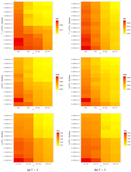
Figure 2. Heat-map for the simulation results of $\gamma$.

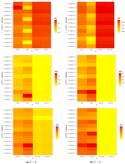
Figure 3. Heat-map for the simulation results of $\sigma$.

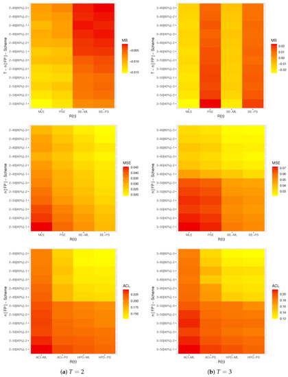
Figure 4. Heat-map for the simulation results of $R\left(t\right)$.

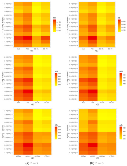
Figure 5. Heat-map for the simulation results of $h\left(t\right)$.

In each heat-map, the ‘$\mathsf{x-lab}$’ represents the proposed estimation procedures, while the ‘$\mathsf{y-lab}$’ represents the censoring input which denoted by ‘$T-n\left[FP\right]$-Scheme’. The colors in each heat-map ranged from yellow to red. For example, in the MBs for $\gamma$ in Figure 2, when the color looks yellow, it means the MB is low, but red indicates the MB is high. As Supplementary Materials, the numerical outcomes of $\gamma$, $\sigma$, $R\left(t\right)$, and $h\left(t\right)$ are reported. For simplification; some notations are used: (i) Bayes estimates from the likelihood function such as “BE-ML”, (ii) Bayes estimates from the product of spacing function such as “BE-PS”, (iii) HPD interval estimates from likelihood function such as “HPD-ML”, and (iv) Bayes estimates from the product of spacing function, such as “HPD-PS”.

4.2. Simulation Discussions

In terms of the lowest MB, MSE, and ACL values, from Figure 2, Figure 3, Figure 4 and Figure 5, this subsection reports useful observations for the behavior of the suggested point and interval estimations of $\gamma$, $\sigma$, $R\left(t\right)$, and $h\left(t\right)$:

• All proposed estimates of $\gamma$, $\sigma$, $R\left(t\right)$ and $h\left(t\right)$ perform satisfactorily.
• As n increases, the offered estimates of $\gamma$, $\sigma$, $R\left(t\right)$, and $h\left(t\right)$ behave well. An identical result is noted when $n-m$ is narrowed down.
• As T increases, we have observed that

  -

  The MBs, MSEs and ACLs for all suggested estimates of $\gamma$, $\sigma$, and $h\left(t\right)$ decrease.

  -

  The MBs and MSEs for all suggested estimates of $R\left(t\right)$ increase while the ACLs of the same parameter decrease.

• Comparing the suggested point/interval inferential techniques, it is clear that

  -

  The MBs, MSEs, and ACLs for all suggested estimates of $\gamma$, $\sigma$, and $h\left(t\right)$ decrease.

  -

  In evaluating $\gamma$ and $R\left(t\right)$, the PS method (and BE-PS method) provides more accurate results than the ML method.

  -

  In evaluating $\sigma$ and $h\left(t\right)$, the ML method (and BE-ML method) provides more accurate results than the PS method.

• Comparing the suggested censoring designs, it is clear that

  -

  The acquired point estimates of $\gamma$ and $R\left(t\right)$ behaved well using right censoring, while those of $\sigma$ and $h\left(t\right)$ behaved well using left censoring.

  -

  The acquired interval estimates of $\gamma$, $R\left(t\right)$, and $h\left(t\right)$ behaved well based on right censoring, while those of $\sigma$ behaved well based on left censoring.

• In summary, in the presence of data created from the proposed adaptive progressively Type-II hybrid mechanism, using the Bayes MH technique through the product of the spacings approach to evaluate the scale and reliability parameters is recommended, while the Bayes MH technique through the likelihood function is also recommended to estimate the shape and hazard parameters.

5. Mechanical Data Analysis

To exhibit the adaptation of proposed approaches to a real-world phenomenon, one real-life engineering data set consisting of thirty failures of repairable mechanical equipment (RME) items is examined. This application demonstrated that the offered model furnishes a better fit than other eight-lifetime models in the literature and that the suggested inferential approaches are effective and simple to use. The RME data was originally reported by Murthy [21] and re-analyzed by Alotaibi et al. [22].

Before calculating the offered estimators, the WE’s fit is compared against eight competitive models, viz., namely:

• Weibull (W$(\gamma ,\sigma )$) by Weibull [23];
• Gamma (G$(\gamma ,\sigma )$) by Johnson et al. [24];
• Nadarajah–Haghighi (NH$(\gamma ,\sigma )$) by Nadarajah and Haghighi [25];
• Weighted Nadarajah–Haghighi (WNH$(\gamma ,\sigma )$) by Khan et al. [26];
• Alpha-power exponential (APE$(\gamma ,\sigma ,\theta )$) by Mahdavi and Kundu [27];
• Weibull-exponential (W-Ex$(\gamma ,\sigma ,\theta )$) by Oguntunde et al. [28];
• Generalized gamma (GG$(\gamma ,\sigma ,\theta )$) by Stacy [29];
• Generalized beta (GB$(\gamma ,\sigma ,\theta ,\tau )$) by McDonald and Xu [30].

For each considered model, the MLEs $\widehat{\gamma }$, $\widehat{\sigma }$, and $\widehat{\theta }$ of $\gamma$, $\sigma$, and $\theta$, respectively, along with their standard-errors (SEs), based on the full RME data, are evaluated and listed in Table 1. Comparing the WE and its competitive lifetime models is conducted based on several criteria, namely: (i) Akaike ($\mathcal{A}$); (ii) Bayesian ($\mathcal{B}$); (iii) consistent Akaike ($\mathcal{CA}$); (iv) Hannan-Quinn ($\mathcal{HQ}$); (v) Cramér-von Mises ($\mathcal{CM}$); (vi) Anderson-Darling ($\mathcal{AD}$); (vii) estimated negative log-likelihood (ENL); and (viii) Kolmogorov-Smirnov ($\mathcal{KS}$) distance (along its p value), see Table 1. It exhibits that the WE model has the lowest values for all given statistics except the highest p value; thus, we can decide that it is the best choice among all the others. It should also be noted that the two most competitive lifetime models in relation to the proposed WE model are the G and GG models. Several plots, called fitted PDFs, fitted RFs, and probability-probability (P-P) plots for the WE and the other competing distributions, are provided in Figure 6 and Figure 7. As a result, the plots shown in Figure 6 and Figure 7 supported the same results as presented in Table 1.

Table 1. Fitting results of WE and its competitive models from RME data.

Model	Est.	$\mathit{\gamma }$	$\mathit{\sigma }$	$\mathit{\theta }$	$\mathit{\tau }$	$\mathcal{A}$	$\mathcal{CA}$	$\mathcal{B}$	ENL	$\mathcal{KS}$ (p Value)
	SE					$\mathcal{HQ}$	$\mathcal{CM}$	$\mathcal{AD}$
WE	Est.	0.3566	1.6558	-	-	83.246	86.048	83.690	39.623	0.0639 (0.9997)
	SE	1.1675	1.8350	-	-	84.142	0.1386	0.0183
W	Est.	1.4633	1.7100	-	-	83.821	86.623	84.265	39.910	0.0749 (0.9960)
	SE	0.2029	0.2254	-	-	84.717	0.2115	0.0280
G	Est.	1.9750	0.7813	-	-	83.259	86.062	83.704	39.630	0.0675 (0.9992)
	SE	0.4737	0.2132	-	-	84.156	0.1443	0.0190
NH	Est.	4.4288	0.0981	-	-	86.308	89.110	86.752	41.154	0.1132 (0.8365)
	SE	6.6965	0.1699	-	-	87.204	0.3531	0.0482
WNH	Est.	1.4906	0.4965	-	-	85.476	88.278	85.920	40.738	0.0958 (0.9457)
	SE	0.7222	0.3618	-	-	86.372	0.2973	0.0404
APE	Est.	2.1234	1.0032	-	-	83.938	86.740	84.382	39.969	0.0788 (0.9923)
	SE	0.5874	0.2014	-	-	84.834	0.1904	0.0254
WEx	Est.	1.4060	32.977	0.0461	-	86.052	90.256	86.975	40.026	0.0822 (0.9873)
	SE	0.1949	61.054	0.0530	-	87.397	0.2406	0.0320
GG	Est.	0.6736	2.0508	0.9569	-	85.273	89.477	86.196	39.637	0.0642 (0.9995)
	SE	0.9012	0.7512	0.4780	-	86.618	0.1412	0.0186
GB	Est.	5.8820	6.0032	0.3770	8.5371	87.425	93.030	89.025	39.713	0.0711 (0.9981)
	SE	63.888	6.7949	3.3153	5.3673	89.218	0.2013	0.0264

Figure 6. Fitted PDFs (left) and RFs (right) of WE and its competitive distributions from RME data.

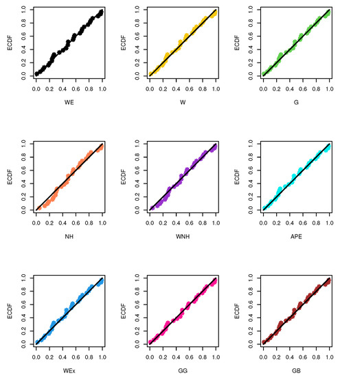
Figure 7. The P-P plots of WE and its competitive distributions from RME data.

Taking $m=10$ and various choices of $\underline{\mathbf{R}}$ and T, from Table 2, three artificial T2APH samples are created, as shown in Table 3. At $t=5$, all estimators of $R\left(t\right)$ and $h\left(t\right)$ are calculated. Due to the fact that we do not have any prior knowledge on $\gamma$, $\sigma$, the the Bayes estimates through both LF and PS functions, using improper gamma priors, are developed. Following Algorithm 1, the first 10,000 of 50,000 MCMC iterations for each unknown parameter, are ignored. For running the MCMC algorithm, the acquired MLE (or PSE) values of $\gamma$, $\sigma$ are considered initial guesses. Then, for each Si for $i=1,2,3,$ the Bayesian and frequentist estimates (with their SEs) as well as 95% ACI/HPD (from LF and PS approaches) estimates (with their widths) of $\gamma$, $\sigma$, $R\left(t\right)$, and $h\left(t\right)$ are calculated, as shown in Table 4. It points out that the Bayes (or HPD interval) estimates of $\gamma$, $\sigma$, $R\left(t\right)$, or $h\left(t\right)$ performed superiorly compared to the conventional approaches.

Table 2. Failure times of repairable mechanical equipment items.

0.11	0.30	0.40	0.45	0.59	0.63	0.70	0.71	0.74	0.77
0.94	1.06	1.17	1.23	1.23	1.24	1.43	1.46	1.49	1.74
1.82	1.86	1.97	2.23	2.37	2.46	2.63	3.46	4.36	4.73

Table 3. Three artificial T2APH samples from RME data.

Si	$\underline{\mathbf{R}}$	$\mathit{T}\left(\mathit{m}\right)$	${\mathit{R}}_{\mathit{m}}^{*}$	Data
S1	$(5^4,0^6)$	0.25(1)	15	0.11, 0.30, 0.40, 0.59, 0.63, 0.70, 0.71, 0.77, 0.94, 1.06
S2	$(0^3,5^4,0^3)$	0.62(5)	10	0.11, 0.30, 0.40, 0.45, 0.59, 0.63, 0.70, 0.77, 0.94, 1.23
S3	$(0^6,5^4)$	0.85(9)	5	0.11, 0.30, 0.40, 0.45, 0.59, 0.63, 0.70, 0.71, 0.74, 0.94

Table 4. Acquired estimates of $\gamma$, $\sigma$, $R\left(t\right)$ and $h\left(t\right)$ from RME data.

Sample	Par.	MLE		BE-ML		ACI-ML			HPD-ML
		PSE		BE-PS		ACI-PS			HPD-PS
		Est.	SE	Est.	SE	Lower	Upper	Width	Lower	Upper	Width
S1	$\gamma$	1.2840	1.3534	1.2839	0.0647	0.0000	3.9367	3.9367	1.2799	1.2878	0.0079
		1.1859	1.0600	1.1859	0.0020	0.0000	3.2636	3.2636	1.1855	1.1863	0.0008
	$\sigma$	0.0137	2.1096	0.0133	0.0997	0.0000	4.1484	4.1484	0.0095	0.0174	0.0079
		0.0256	1.7973	0.0256	0.0020	0.0000	3.5483	3.5483	0.0252	0.0260	0.0008
	$R\left(0.5\right)$	0.8626	0.0440	0.8627	0.0041	0.7764	0.9488	0.1724	0.8619	0.8635	0.0016
		0.8779	0.0422	0.8779	0.0004	0.7953	0.9606	0.1652	0.8779	0.8780	0.0002
	$h\left(0.5\right)$	0.5076	0.1639	0.5074	0.0153	0.1863	0.8288	0.6426	0.5044	0.5103	0.0060
		0.4506	0.1560	0.4506	0.0014	0.1449	0.7564	0.6115	0.4503	0.4509	0.0006
S2	$\gamma$	0.6827	0.2495	0.6826	0.0199	0.1937	1.1717	0.9779	0.6786	0.6864	0.0078
		0.6822	0.6062	0.6822	0.0020	0.0000	1.8704	1.8704	0.6818	0.6826	0.0008
	$\sigma$	6.7542	8.8738	6.7541	0.0201	0.0000	24.147	24.147	6.7501	6.7580	0.0079
		2.5485	8.1290	2.5485	0.0020	0.0000	18.481	18.481	2.5481	2.5489	0.0008
	$R\left(0.5\right)$	0.8056	0.0686	0.8056	0.0073	0.6712	0.9399	0.2687	0.8042	0.8070	0.0029
		0.8730	0.0503	0.8730	0.0006	0.7744	0.9716	0.1973	0.8729	0.8731	0.0002
	$h\left(0.5\right)$	0.6226	0.1943	0.6225	0.0222	0.2418	1.0035	0.7617	0.6182	0.6269	0.0087
		0.4493	0.1537	0.4493	0.0020	0.1481	0.7504	0.6023	0.4489	0.4497	0.0008
S3	$\gamma$	1.2658	0.4403	1.2658	0.0020	0.4028	2.1288	1.7260	1.2654	1.2662	0.0008
		1.1785	1.0408	1.1785	0.0020	0.0000	3.2185	3.2185	1.1781	1.1789	0.0008
	$\sigma$	0.0009	0.5677	0.0008	0.0021	0.0000	1.1135	1.1135	0.0004	0.0012	0.0008
		0.0018	0.9168	0.0017	0.0020	0.0000	1.7987	1.7987	0.0014	0.0021	0.0008
	$R\left(0.5\right)$	0.8671	0.0425	0.8671	0.0004	0.7837	0.9504	0.1667	0.8670	0.8671	0.0002
		0.8815	0.0877	0.8815	0.0004	0.7096	1.0533	0.3438	0.8814	0.8815	0.0001
	$h\left(0.5\right)$	0.4909	0.1581	0.4909	0.0015	0.1810	0.8008	0.6198	0.4906	0.4912	0.0006
		0.4376	0.3242	0.4376	0.0014	0.0000	1.0730	1.0730	0.4373	0.4379	0.0006

To demonstrate the existence and uniqueness of ML (or PS) estimates, developed from the RME data, Figure 8 displays the profile plots from log-LF and log-PS of $\gamma$ and $\sigma$. It demonstrates that the acquired maximum likelihood and product of spacing estimates of $\gamma$ and $\sigma$ exist and are unique.

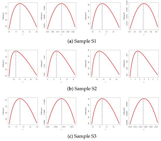
Figure 8. The profile log-LF (left) and profile log-PS (right) of $\gamma$ and $\sigma$ from RME data.

In Table 5, several properties of $\gamma$, $\sigma$, $R\left(t\right)$, and $h\left(t\right)$ based on the remaining 40,000 MCMC iterations namely: mean, mode, three quartiles $Q_i,i=1,2,3$, standard deviation (SD) and skewness (Skew.) are listed.

Table 5. Properties of MCMC iterations of $\gamma$, $\sigma$, $R\left(t\right)$ and $h\left(t\right)$ from RME data.

Sample	Par.	Mean	Mode	${\mathit{Q}}_1$	${\mathit{Q}}_2$	${\mathit{Q}}_3$	SD	Skew.
Bayes LF-based
S1	$\gamma$	1.2839	1.2825	1.2826	1.2839	1.2853	0.0020	$-0.0066$
	$\sigma$	0.0133	0.0072	0.0120	0.0133	0.0147	0.0020	0.0003
	$R\left(0.5\right)$	0.8627	0.8628	0.8624	0.8627	0.8629	0.0004	0.0150
	$h\left(0.5\right)$	0.5074	0.5053	0.5063	0.5074	0.5084	0.0015	$-0.0145$
S2	$\gamma$	0.6826	0.6785	0.6813	0.6826	0.6840	0.0020	0.0159
	$\sigma$	6.7541	6.7498	6.7528	6.7541	6.7555	0.0020	0.0219
	$R\left(0.5\right)$	0.8056	0.8058	0.8051	0.8056	0.8061	0.0007	$-0.0152$
	$h\left(0.5\right)$	0.6225	0.6178	0.6210	0.6225	0.6240	0.0022	0.0153
S3	$\gamma$	1.2658	1.2658	1.2656	1.2658	1.2659	0.0002	$-0.0027$
	$\sigma$	0.0008	0.0002	0.0007	0.0008	0.0010	0.0002	0.0153
	$R\left(0.5\right)$	0.8671	0.8671	0.8670	0.8671	0.8671	0.0000	0.0038
	$h\left(0.5\right)$	0.4909	0.4907	0.4908	0.4909	0.4910	0.0001	$-0.0038$
Bayes PS-based
S1	$\gamma$	1.1859	1.1859	1.1858	1.1859	1.1861	0.0002	0.0138
	$\sigma$	0.0256	0.0254	0.0255	0.0256	0.0258	0.0002	0.0180
	$R\left(0.5\right)$	0.8779	0.8779	0.8779	0.8779	0.8780	0.0000	$-0.0076$
	$h\left(0.5\right)$	0.4506	0.4505	0.4505	0.4506	0.4507	0.0001	0.0076
S2	$\gamma$	0.6822	0.6821	0.6821	0.6822	0.6823	0.0002	0.0143
	$\sigma$	2.5485	2.5485	2.5484	2.5485	2.5487	0.0002	0.0182
	$R\left(0.5\right)$	0.8730	0.8730	0.8730	0.8730	0.8730	0.0001	$-0.0143$
	$h\left(0.5\right)$	0.4493	0.4492	0.4491	0.4493	0.4494	0.0002	0.0144
S3	$\gamma$	1.1785	1.1782	1.1784	1.1785	1.1787	0.0002	0.0100
	$\sigma$	0.0017	0.0013	0.0016	0.0017	0.0019	0.0002	0.0210
	$R\left(0.5\right)$	0.8815	0.8815	0.8814	0.8815	0.8815	0.0000	$-0.0075$
	$h\left(0.5\right)$	0.4376	0.4372	0.4375	0.4376	0.4377	0.0001	0.0076

To highlight the performance for 40,000 MCMC draws (from LF and PS) of $\gamma$, $\sigma$, $R\left(t\right)$, and $h\left(t\right)$, both trace and density (with Gaussian line) plots from S1 (as an example) are displayed in Figure 9. In both trace and density plots, the Bayes estimate is expressed by a soled (—) horizontal line, whereas the 95% HPD interval limits are mentioned by dashed (- - -) horizontal lines. Other density and trace diagrams for samples Si for $i=2,3$ are also plotted and provided in the supplementary file for brevity. Figure 9 indicates that the proposed Bayes-MH technique, in both LF-based and PS-based approaches, converges adequately. It also shows that, for all given samples, the simulated marginal posterior density estimates of $\gamma$, $\sigma$, $R\left(t\right)$, or $h\left(t\right)$ behave in a symmetric manner.

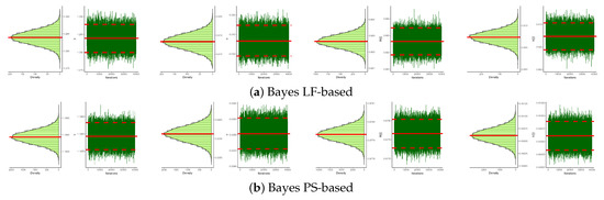
Figure 9. Density (left) and Trace (right) diagrams of $\gamma$, $\sigma$, $R\left(t\right)$ and $h\left(t\right)$ based on S1 from RME data.

As a result, using LF and PS methodologies in the presence of the T2APH mechanism, the numerical outcomes of the offered estimates of $\gamma$, $\sigma$, $R\left(t\right)$, and $h\left(t\right)$ using the RME data set furnish a significant examination of the WE lifespan model.

6. Conclusions

This paper investigates the maximum likelihood and product of spacing estimators of unknown weighted-exponential parameters of life using an adaptive progressive Type-II hybrid plan. Under the premise of independent gamma priors, using the squared-error loss, the Bayes estimators according to both the likelihood and product of spacing functions have been derived. Because the Bayes estimators have not been offered in closed formulas, the MH process has been suggested. Two types of intervals for the unknown quantities, through approximate confidence as well as the highest posterior density methods, have also been calculated. To compare the efficiency of the acquired estimates, different Monte Carlo simulations have been provided. A real-world data set of repairable mechanical equipment items has been analyzed to illustrate the adaptability of the offered model in a real-world scenario and to confirm how our estimates may be used in practice. We believe that data analysts and reliability practitioners will find the findings and approach covered in this paper useful. Finally, the methodologies offered in this article may be extended in future research to include competing risks, accelerated life tests, other censoring strategies, etc.

References

- Balakrishnan, N.; Cramer, E. The Art of Progressive Censoring; Springer: Birkhäuser, NY, USA, 2014. [Google Scholar]
- Kundu, D.; Joarder, A. Analysis of Type-II progressively hybrid censored data. Comput. Stat. Data Anal. 2006, 50, 2509–2528. [Google Scholar] [CrossRef]
- Ng, H.K.T.; Kundu, D.; Chan, P.S. Statistical analysis of exponential lifetimes under an adaptive Type-II progressive censoring scheme. Nav. Res. Logist. 2009, 56, 687–698. [Google Scholar] [CrossRef]
- Elshahhat, A.; Nassar, M. Bayesian survival analysis for adaptive Type-II progressive hybrid censored Hjorth data. Comput. Stat. 2021, 36, 1965–1990. [Google Scholar] [CrossRef]
- Elshahhat, A.; Nassar, M. Analysis of adaptive Type-II progressively hybrid censoring with binomial removals. J. Stat. Comput. Simul. 2023, 93, 1077–1103. [Google Scholar] [CrossRef]
- Cheng, R.C.H.; Amin, N.A.K. Estimating parameters in continuous univariate distributions with a shifted origin. J. R. Stat. Soc. Ser. B 1983, 45, 394–403. [Google Scholar] [CrossRef]
- Ranneby, B. The maximum spacing method. An estimation method related to the maximum likelihood method. Scand. J. Stat. 1984, 11, 93–112. [Google Scholar]
- Anatolyev, S.; Kosenok, G. An alternative to maximum likelihood based on spacings. Econom. Theory 2005, 21, 472–476. [Google Scholar] [CrossRef]
- El-Sherpieny, E.S.A.; Almetwally, E.M.; Muhammed, H.Z. Progressive Type-II hybrid censored schemes based on maximum product spacing with application to Power Lomax distribution. Physica A Stat. Mech. Its Appl. 2020, 553, 124251. [Google Scholar] [CrossRef]
- Gupta, R.D.; Kundu, D. A new class of weighted exponential distributions. Statistics 2009, 43, 621–634. [Google Scholar] [CrossRef]
- Dey, S.; Ali, S.; Park, C. Weighted exponential distribution: Properties and different methods of estimation. J. Stat. Comput. Simul. 2015, 85, 3641–3661. [Google Scholar] [CrossRef]
- Farahani, Z.S.M.; Khorram, E. Bayesian statistical inference for weighted exponential distribution. Commun. Stat.-Simul. Comput. 2014, 43, 1362–1384. [Google Scholar] [CrossRef]
- Tian, Y.; Gui, W. Inference of weighted exponential distribution under progressively Type-II censored competing risks model with electrodes data. J. Stat. Comput. Simul. 2021, 91, 3426–3452. [Google Scholar] [CrossRef]
- Henningsen, A.; Toomet, O. maxLik: A package for maximum likelihood estimation in R. Comput. Stat. 2011, 26, 443–458. [Google Scholar] [CrossRef]
- Lawless, J.F. Statistical Models and Methods For Lifetime Data, 2nd ed.; John Wiley and Sons: Hoboken, NJ, USA, 2003. [Google Scholar]
- Greene, W.H. Econometric Analysis, 4th ed.; Prentice-Hall: Hoboken, NJ, USA, 2000. [Google Scholar]
- Gelman, A.; Carlin, J.B.; Stern, H.S.; Rubin, D.B. Bayesian Data Analysis, 2nd ed.; Chapman and Hall/CRC: Boca Raton, FL, USA, 2004. [Google Scholar]
- Lynch, S.M. Introduction to Applied Bayesian Statistics and Estimation for Social Scientists; Springer: Birkhäuser, NY, USA, 2007. [Google Scholar]
- Chen, M.H.; Shao, Q.M. Monte Carlo estimation of Bayesian credible and HPD intervals. J. Comput. Graph. Stat. 1999, 8, 69–92. [Google Scholar]
- Plummer, M.; Best, N.; Cowles, K.; Vines, K. CODA: Convergence diagnosis and output analysis for MCMC. R News 2006, 6, 7–11. [Google Scholar]
- Murthy, D.N.P.; Xie, M.; Jiang, R. Weibull Models; Wiley Series in Probability and Statistics; Wiley: Hoboken, NJ, USA, 2004. [Google Scholar]
- Alotaibi, R.; Nassar, M.; Elshahhat, A. Estimations of modified Lindley parameters using progressive Type-II censoring with applications. Axioms 2023, 12, 171. [Google Scholar] [CrossRef]
- Weibull, W. A statistical distribution function of wide applicability. J. Appl. Mech. 1951, 18, 293–297. [Google Scholar] [CrossRef]
- Johnson, N.; Kotz, S.; Balakrishnan, N. Continuous Univariate Distributions, 2nd ed.; John Wiley and Sons: Hoboken, NJ, USA, 1994. [Google Scholar]
- Nadarajah, S.; Haghighi, F. An extension of the exponential distribution. Statistics 2011, 45, 543–558. [Google Scholar] [CrossRef]
- Khan, M.N.; Saboor, A.; Cordeiro, G.M.; Nazir, M.; Pescim, R.R. A weighted Nadarajah and Haghighi distribution. UPB Sci. Bull. Ser. A Appl. Math. Phys. 2018, 80, 133–140. [Google Scholar]
- Mahdavi, A.; Kundu, D. A new method for generating distributions with an application to exponential distribution. Commun. Stat.-Theory Methods 2017, 46, 6543–6557. [Google Scholar] [CrossRef]
- Oguntunde, P.E.; Balogun, O.S.; Okagbue, H.I.; Bishop, S.A. The Weibull-exponential distribution: Its properties and applications. J. Appl. Sci. 2015, 15, 1305–1311. [Google Scholar] [CrossRef]
- Stacy, E.W. A Generalization of the Gamma Distribution. Ann. Math. Stat. 1962, 33, 1187–1192. [Google Scholar] [CrossRef]
- McDonald, J.B.; Xu, Y.J. A generalization of the beta distribution with applications. J. Econom. 1995, 66, 133–152. [Google Scholar] [CrossRef]
Disclaimer/Publisher’s Note: The statements, opinions and data contained in all publications are solely those of the individual author(s) and contributor(s) and not of MDPI and/or the editor(s). MDPI and/or the editor(s) disclaim responsibility for any injury to people or property resulting from any ideas, methods, instructions or products referred to in the content. |
© 2023 by the authors. Licensee MDPI, Basel, Switzerland. This article is an open access article distributed under the terms and conditions of the Creative Commons Attribution (CC BY) license (https://creativecommons.org/licenses/by/4.0/).