Lyapunov Functionals in Integral Equations

Abstract

Lyapunov functions/functionals have found their footing in Volterra integro-differential equations. This is not the case for integral equations, and it is therefore further explored in this paper. In this manuscript, we utilize Lyapunov functionals combined with Laplace transform to qualitatively analyze the solutions of the integral equation In addition, we extend our method to nonlinear integral equations, integral equations with infinite delay, and integral equations with several kernels. We mention that Laplace transform has been used to solve integral equations of convolution types but has never been applied directly to integral equations that are not of the convolution type. In addition, our method allows us to find the upper estimates, and our necessary conditions are easy to verify.

1. Introduction

Lyapunov functions/functionals have a long history of successful use in ordinary differential equations, functional differential equations, and Volterra integro-differential equations. The literature is vast, and we refer the reader to the most prominent results given in [1,2,3,4,5,6,7,8]. Most scientific fields are directly or indirectly involved with differential or integral equations. Additionally, a lot of the issues call for quite precise qualitative outcomes. In particular, it is imperative to consider the following issues when dealing with certain problems, for example, in the case that a convenient approximation cannot be used in place of the function. Moreover, it is of great benefit to understand how each solution behaves as well as understand how solutions behave over a very long period of time. It is challenging to achieve all three requirements, even with the most sophisticated computational techniques. However, A. M. Lyapunov, a Russian mathematician, developed a straightforward approach that satisfied those requirements for ordinary differential equations more than a century ago. His approach is now known as the “Lyapunov direct method”.

Many researchers differentiate an integral equation before using Lyapunov’s direct approach on it. Miller, in [7], considered a system of integral equations transferred to a system of integro-differential equations and used the notion of the Lyapunov direct method to analyze the solutions. The given functions are not differentiable, which makes this procedure complex and challenging. Furthermore, it is well known that differentiation causes roughness, whereas integration produces smoothness; as a result, differentiation might produce results that might not be applicable to or even hold for the original problem. T. A. Burton in [1] compiled a collection of recent results and papers on integral equations. His work contains clever ways of constructing Lyapunov functions/functionals for integral equations. Burton utilizes Lyapunov functionals along with the resolvent to arrive at boundedness and stability results. In [9], the authors extended some of the arguments of [1] to Caputo integral equations and arrived at boundedness and stability results. Researchers and scientists periodically use Laplace transform to solve an integral equation of the convolution type. No one up till now has been able to use Laplace transform on integral equations that are not of convolution type. That is why we believe that the results of this this paper are significant and innovative.

As we have mentioned, the Lyapunov method is well established in the study of integro-differential equations. For example, in Ref. [10], the authors considered the nonlinear integro-differential equation

$$y^{\prime }\left(t\right)=A\left(t\right)y+f\left(y\right)+{\int }_0^{t}C(t,s)h\left(y\left(s\right)\right)ds+p\left(t\right),y\left(0\right)=y_0,$$

where A, $f\left(y\right)$, p, and $h\left(y\right)$ are scalar functions that are continuous, use Lyapunov functionals combined with Laplace transform, and provide qualitative results concerning the equation’s solution. Our approach is a novel method of analyzing solutions to integral equations. This, by itself, should spark an outburst of new research in integral equations and related topics.

This paper is organized into the following sections. In Section 2, we consider linear equations and utilize Lyapunov functionals combined with Laplace transform and obtain boundedness and existence results concerning solutions. In Section 3, we extend the results of Section 2 to nonlinear integral equations. Section 4 is devoted to integral equations with infinite delay and integral equations with several kernels. Examples will be fully worked out in the relevant sections.

The following is the definition of Laplace transform. We say the function $x\left(t\right)$ is of an exponential order for $t\ge 0,$ if there are constants $m\ge 0$ and c such that

$$\left|x\right|\le m{e}^{ct}forallt\ge 0.$$

Let $x\left(t\right)$ be a piecewise continuous function that is defined for $t\ge 0$ and of exponential order. Then, the Laplace transform $L\left(x\right)\left(s\right)$ of $x\left(t\right)$ is defined by the integral

$$L\left(x\right)\left(s\right)={\int }_0^{+\infty }{e}^{-st}x\left(t\right)dt,$$

where s is a real number chosen so that the improper integral exists.

Below, we briefly introduce the notion of a Lyapunov function/functional. The definitions below are of general types, and hence they can be adjusted to suit different types of differential equations or integral equations. Let D be an open subset of ${\mathbb{R}}^n$ containing $x=0.$ Define

$$V:[0,\infty )\times D\to [0,\infty ),$$

where V is any differentiable scalar function. If ${\displaystyle \zeta :[0,\infty )\to {\mathbb{R}}^n}$ is any differentiable function, then $V\left(t\right):=V(t,\zeta (t\left)\right)$ is a scalar function of t, and using the chain rule we can compute its derivative,

$$V^{\prime }\left(t\right)=\frac{\partial V}{\partial x_1}{\zeta }_1^{\prime }\left(t\right)+\cdots +\frac{\partial V}{\partial x_n}{\zeta }_n^{\prime }\left(t\right)+\frac{\partial V}{\partial t}.$$

For emphasis, let D be an open subset of ${\mathbb{R}}^n$ containing $x=0,$ and ${\displaystyle f:[0,\infty )\times D\to {\mathbb{R}}^n}$ with ${\displaystyle f(t,0)=0.}$ Assume the existence of the unknown solution $x:[0,\infty )\to {\mathbb{R}}^n$ of the system

$$x^{\prime }=f(t,x),$$

(1)

where

$$f(t,x)=\left(\begin{array}{c}{f}_1(t,x)\\ f_2(t,x)\\ ⋮\\ f_n(t,x)\end{array}\right).$$

Thus, x and f are n vectors. Then, it follows from the above argument that

$$\begin{array}{ccc}\hfill V^{\prime }(t,x\left(t\right))& =& \frac{\partial V(t,x(t\left)\right)}{\partial x_1}{f}_1(t,x\left(t\right))+\cdots \hfill \\ & +& \frac{\partial V(t,x(t\left)\right)}{\partial x_n}{f}_n(t,x\left(t\right))+\frac{\partial V}{\partial t}.\hfill \end{array}$$

(2)

Thus, expression (2) defines the derivative of the function $V(t,x)$ along the unknown solutions of (1). Let D be the subset defined above.

Definition 1. 

A continuous autonomous function $V:D\to [0,\infty )$ is positive definite if

$$V\left(0\right)=0\mathit{and}V\left(x\right)>0\mathit{if}x\ne 0.$$

V is said to be negative definite if $-V$ is positive definite.

It is customary to define a Lyapunov function by the next definition. This is the case when the function f in (1) does not explicitly depend on time $t,$ or system (1) is autonomous.

Definition 2. 

Let

$$V:D\to [0,\infty ),$$

have continuous first partial derivatives. If V is positive definite and

$$V^{\prime }\left(x\left(t\right)\right)=\frac{\partial V\left(x\right(t\left)\right)}{\partial x_1}{f}_1\left(x\left(t\right)\right)+\cdots +\frac{\partial V\left(x\right(t\left)\right)}{\partial x_n}{f}_n\left(x\left(t\right)\right)\le 0,$$

for $x\in D$ and $x\ne 0,$ then V is called a Lyapunov function for system (1).

If the inequality is strict, that is, $V^{\prime }\left(x\left(t\right)\right)<0$, then V is said to be a strict Lyapunov function.

For the sake of this paper, we adopt the following definition of a Lyapunov function.

Definition 3. 

Let M and τ be positive constants. Let V be defined as in Definition 2. If

$$V^{\prime }\left(x\left(t\right)\right)\le -\tau \left|x\right|+M,$$

for $x\in D,$ and $x\ne 0,$ then V is called a Lyapunov function for system (1).

The literature on the use of Lyapunov functions/functionals in differential, functional differential equations are vast, and we refer the reader to [1,2,3,4,5,11,12].

For the rest of the paper, we use the notation

$$V\left(t\right):=V\left(x\right(t\left)\right),$$

where x is the unknown solution of (1).

2. Linear Integral Equations

We begin by considering the linear and scalar integral equation

$$y\left(t\right)=a\left(t\right)-{\int }_0^{t}C(t,s)y\left(s\right)ds,$$

(3)

where $y:\mathbb{R}\to \mathbb{R},$ $a:[0,\infty )\to \mathbb{R}$ is continuous and $C:[0,\infty )\times [0,\infty )\to \mathbb{R}$ is continuous for $0\le s\le t<\infty .$ If C and a are differentiable, we can differentiate (3) to obtain a Volterra integro-differential equation, which we can then analyze using the method of [10]. However, because differentiability is such a significant criterion, we might not always have that luxury. We want to be clear that the approach we use in this work is completely distinct from any approach offered in the book [1]. However, for more reading on the subject of Volterra integro-differential equations, we refer to [6,7,8,13,14]. We begin with the following lemma.

Lemma 1. 

Suppose there is a differentiable function ${\displaystyle \psi :[0,\infty )\to (0,\infty )}$ such that

$${\psi }^{\prime }(t-s)\le -\left|C(t,s)\right|,0\le s\le t<\infty ,$$

(4)

and ${\displaystyle 0<\psi \left(0\right)<1.}$ If $y\left(t\right)$ is any solution of (3) and if the Lyapunov function V is defined by

$$V\left(t\right)={\int }_0^t\psi (t-s)\left|y\left(s\right)\right|ds,$$

(5)

then there exists a constant $\alpha \in (0,1),$ such that

$$V^{\prime }\left(t\right)\le -\alpha \left|y\left(t\right)\right|+M,$$

(6)

where

$$\alpha =1-\psi \left(0\right),\mathit{and}M=\underset{t\ge 0}{max}\left|a\left(t\right)\right|.$$

Proof. 

Let V be defined by (5) and $y\left(t\right)$ be a solution of (3). Then, differentiating V with respect to t gives

$$\begin{array}{ccc}\hfill V^{\prime }\left(t\right)& =& \psi \left(0\right)\left|y\left(t\right)\right|+{\int }_0^t{\psi }^{\prime }(t-s)\left|y\left(s\right)\right|ds\hfill \\ & \le & \psi \left(0\right)\left|y\left(t\right)\right|-{\int }_0^t\left|C(t,s)\right|\left|y\left(s\right)\right|ds.\hfill \end{array}$$

(7)

Now, from (3) we have that

$$\left|y\left(t\right)\right|-\left|a\left(t\right)\right|\le {\int }_0^t\left|C(t,s)\right|\left|y\left(s\right)\right|ds.$$

Substituting into (7), we arrive at

$$\begin{array}{c}\hfill V^{\prime }\left(t\right)\le \psi \left(0\right)\left|y\left(t\right)\right|+\left|a\left(t\right)\right|-\left|y\left(t\right)\right|\le -\alpha \left|y\left(t\right)\right|+M.\end{array}$$

□

Proposition 1. 

If ${\displaystyle f:[0,\infty )\to [0,\infty )}$ is uniformly continuous, and ${\displaystyle f\in L^1\left([0,\infty )\right),}$ then

$$\underset{x\to \infty }{lim}f\left(x\right)=0.$$

Proof. 

Suppose the contrary, that is, f does not converge to zero. Then, there is an $ϵ>0$ such that we can define an increasing sequence $x_n$ so that $x_n\to \infty ,$ so we have $f\left(x_n\right)>ϵ.$ Since f is uniformly continuous, $\delta >0$ exists such that

$$|x-y|<\delta ,\mathrm{implies}\mathrm{that}|f\left(x\right)-f\left(y\right)|<\frac{ϵ}{2}.$$

By referring to the subsequence, we may suppose that $x_{n+1}>x_n+1,$ for each $n=1,2,\cdots$ Since the intervals $(x_n,x_n+\delta ),n=k,k+1,\cdots$ are disjointed, we have that

$${\int }_{x_n}^{x_n+\delta }f\left(y\right)dy\ge {\int }_{x_n}^{x_n+\delta }\left[f\left(x_n\right)-\frac{ϵ}{2}\right]dy>\frac{ϵ}{2}\delta .$$

Summing these intervals, we see that

$${\int }_0^{\infty }f\left(x\right)dx=\infty ,$$

which is a contradiction. This completes the proof. □

Lemma 2. 

Let $\beta :[0,\infty )\to [0,\infty )$ be uniformly continuous such that

$${\int }_0^t\{\psi (t-s)+\alpha \}\beta \left(s\right)ds=1,t\ge 0.$$

(8)

Let ψ be defined in Lemma 1 and if

$${\int }_0^{\infty }\psi \left(t\right)dt<\infty ,$$

(9)

then

$$\beta \left(t\right)\in L^1[0,\infty ),$$

(10)

and

$$\beta \left(t\right)\to 0ast\to \infty .$$

Proof. 

Since $\psi >0$ and due to (9), we have from (8) that

$${\int }_0^t\alpha \beta \left(s\right)ds\le 1,$$

or ${\int }_0^t\beta \left(s\right)ds\le \frac{1}{\alpha }.$ Taking the limit at $t\to \infty ,$ we obtain

$$\underset{t\to \infty }{lim}{\int }_0^t\beta \left(s\right)ds\le \frac{1}{\alpha },$$

This proves $\beta \left(t\right)\in L^1[0,\infty ),$ since the term on the right-hand side is independent of $t.$ Since $\beta \ge 0$ for all $t\ge 0,$ uniformly continuous, and $\beta \left(t\right)\in L^1[0,\infty ),$ it follows from Proposition 1 that $\beta \left(t\right)\to 0ast\to \infty .$ This completes the proof. □

Remark 1. 

The results of Lemma 2 imply that a positive constant F exists such that $\beta \left(t\right)\le F.$

Theorem 1. 

Assume the hypotheses of Lemmata 1 and 2 hold. In addition, we assume that β and ψ are of exponential orders. If $y\left(t\right)$ is any solution of (3), then

$$\left|y\left(t\right)\right|\le \frac{M}{\alpha }.$$

Proof. 

Let ∗ denote the convolution between two functions. By taking the Laplace transform in (8), we arrive at

$$L({\int }_0^t\psi (t-s)\beta \left(s\right)ds)+L({\int }_0^t\alpha \beta \left(s\right)ds)=L\left(1\right).$$

Or,

$$L(\psi \ast \beta )+\alpha L(1\ast \beta )=\frac{1}{s}.$$

In particular,

$$L\left(\psi \right)L\left(\beta \right)+\alpha L\left(1\right)L\left(\beta \right)=\frac{1}{s}.$$

Solving for $L\left(\beta \right)$ gives

$$L\left(\beta \right)=\frac{1}{(L\left(\psi \right)+\alpha \frac{1}{s})s}.$$

(11)

Due to (6), there is a non-negative function $\eta :[0,\infty )\to [0,\infty )$ that is of exponential order such that

$$V^{\prime }\left(t\right):=-\alpha \left|y\right|+M-\eta \left(t\right).$$

Taking the Laplace transform and using $V\left(0\right)=0,$ we arrive at

$$sL\left(V\right)=-\alpha L\left(\right|y\left|\right)+\frac{M}{s}-L\left(\eta \right).$$

This yields

$$L\left(V\right)=\left[-\alpha L\left(\right|y\left|\right)+\frac{M}{s}-L\left(\eta \right)\right]\frac{1}{s}.$$

Taking the Laplace transform in (5), we obtain

$$L\left(V\right)=L\left(\psi \right)L\left(\right|y\left|\right).$$

Comparing the last two expressions and solving for $L\left(\right|y\left|\right)$, we obtain

$$\begin{array}{ccc}\hfill L\left(\right|y\left|\right)& =& \frac{\frac{M}{s}-L\left(\eta \right)}{\alpha +sL\left(\psi \right)}\hfill \\ & =& \frac{\frac{M}{s}-L\left(\eta \right)}{[\frac{\alpha }{s}+L\left(\psi \right)]s}\hfill \\ & =& [\frac{M}{s}-L\left(\eta \right)]L\left(\beta \right)\hfill \\ & =& L\left(\beta \right)\frac{M}{s}-L\left(\eta \right)L\left(\beta \right)\hfill \\ & =& L\left({\int }_0^{t}M\beta \left(s\right)ds\right)-L\left({\int }_0^t\eta (t-s)\beta \left(s\right)ds\right).\hfill \end{array}$$

(12)

Taking the inverse Laplace transform in (12), we obtain

$$\left|y\right|=M{\int }_0^t\beta \left(s\right)ds-{\int }_0^t\eta (t-s)\beta \left(s\right)ds$$

or

$$\left|y\left(t\right)\right|\le M{\int }_0^t\beta \left(s\right)ds\le \frac{M}{\alpha }.$$

This completes the proof. □

We display the following simple example. Note that the figures accompanying the several examples are numerically approximated. The approximate solutions are obtained using the iterative method,

$$y_{n+1}\left(t\right)=a\left(t\right)+{\int }_a^{b}C(x,s)y_n\left(s\right)ds,n=0,1,...,$$

(13)

where $y_0\left(x\right)=a\left(t\right)$. The sequence converges to the approximate solution as the number of iterations approaches ∞.

Example 1. 

Consider the integral equation

$$y\left(t\right)=cos\left(t\right)-{\int }_0^t\frac{1}{{(t+2-s)}^3}y\left(s\right)ds.$$

(14)

Then, we have ${\displaystyle a\left(t\right)=cos\left(t\right)\mathit{and}C(t,s)=\frac{1}{{(t+2-s)}^3}.}$ Set ${\displaystyle \psi \left(t\right)=\frac{1}{{(t+2)}^2}.}$ Then, it follows that

$${\int }_0^{\infty }\frac{1}{{(t+2)}^2}dt<\infty .$$

In addition, ${\psi }^{\prime }\left(t\right)=-\frac{2}{{(t+2)}^3}$ and hence

$$-\frac{2}{{(t+2-s)}^3}={\psi }^{\prime }(t-s)<-\frac{1}{{(t+2-s)}^3}=-\left|C(t,s)\right|.$$

Moreover,

$$\alpha =1-\psi \left(0\right)=1-\frac{1}{4}=\frac{3}{4}\in (0,1).$$

Thus, by Theorem 1 any solution $y\left(t\right)$ of (14) satisfies

$$\left|y\left(t\right)\right|\le \frac{M}{\alpha }=\frac{4}{3},$$

since $M={max}_{t\ge 0}|cos\left(t\right)|=1.$

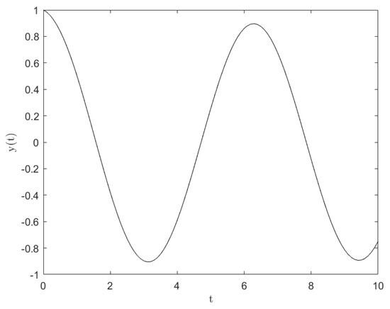
We refer to Figure 1. for the upper bound on the solution.

Figure 1. Using MATLAB, the graph shows that the upper bound of this approximation at $t=0$ is 1.

3. Nonlinear Integral Equations

Now, we extend the results of Section 2 to the nonlinear and scalar integral equations of the form

$$y\left(t\right)=a\left(t\right)-{\int }_0^{t}C(t,s)h\left(y\left(s\right)\right)ds,$$

(15)

where the continuity of a and C are the same as in Section 2 and the function h is continuous in y and satisfies the growth condition

$$\left|h\right(y\left)\right|\le \lambda \left|y\right|,$$

(16)

for positive constant $\lambda .$ The transition from the linear case to nonlinear case is not difficult, but nevertheless some of the details must be provided. The next lemma is parallel to Lemma 1.

Lemma 3. 

Assume (16), and suppose there is a differentiable function ${\displaystyle \psi :[0,\infty )\to (0,\infty )}$ such that

$${\psi }^{\prime }(t-s)\le -\left|C(t,s)\right|,0\le s\le t<\infty ,$$

(17)

and ${\displaystyle 0<\psi \left(0\right)<1.}$ If $y\left(t\right)$ is any solution of (15) and if the Lyapunov function V is defined by

$$V\left(t\right)=\lambda {\int }_0^t\psi (t-s)\left|y\left(s\right)\right|ds,$$

(18)

then a constant $\alpha \in (0,1),$ exists such that

$$V^{\prime }\left(t\right)\le -\alpha \left|y\left(t\right)\right|+M,$$

(19)

where such that

$$\alpha =1-\lambda \psi \left(0\right),\mathit{and}M=\underset{t\ge 0}{max}\left|a\left(t\right)\right|.$$

Proof. 

Let V be defined by (18) and $y\left(t\right)$ be a solution of (15). Then, differentiating V with respect to t gives

$$\begin{array}{ccc}\hfill V^{\prime }\left(t\right)& \le & \lambda \psi \left(0\right)\left|y\left(t\right)\right|+\lambda {\int }_0^t{\psi }^{\prime }(t-s)\left|y\left(s\right)\right|ds\hfill \\ & \le & \lambda \psi \left(0\right)\left|y\left(t\right)\right|-\lambda {\int }_0^t\left|C(t,s)\right|\left|y\left(s\right)\right|ds.\hfill \end{array}$$

(20)

Now, from (15) we have that

$$\left|y\left(t\right)\right|-\left|a\left(t\right)\right|\le \lambda {\int }_0^t\left|C(t,s)\right|\left|y\left(s\right)\right|ds.$$

Substituting into (20), we arrive at

$$\begin{array}{c}\hfill V^{\prime }\left(t\right)\le \lambda \psi \left(0\right)\left|y\left(t\right)\right|+\left|a\left(t\right)\right|-\left|y\left(t\right)\right|\le -\alpha \left|y\left(t\right)\right|+M.\end{array}$$

□

Similarly, the next lemma is parallel to Lemma 2. Its proof is identical to Lemma 1, and it will be omitted.

Lemma 4. 

Assume (9), and let $\beta \left(t\right)\ge 0$ be a scalar function that is uniformly continuous on $[0,\infty )$ and be defined by

$${\int }_0^t\{\lambda \psi (t-s)+\alpha \}\beta \left(s\right)ds=1.$$

(21)

Then,

$$\beta \left(t\right)\in L^1[0,\infty ),$$

and

$$\beta \left(t\right)\to 0ast\to \infty .$$

We state our results in the next theorem, which is parallel to Theorem 1.

Theorem 2. 

Assume the hypotheses of Lemmata 3 and 4 hold. If $y\left(t\right)$ is any solution of (15), then

$$\left|y\left(t\right)\right|\le \frac{M}{\alpha }.$$

Proof. 

By taking the Laplace transform in (21), we arrive at

$$\lambda L({\int }_0^t\psi (t-s)\beta \left(s\right)ds)+L({\int }_0^t\alpha \beta \left(s\right)ds)=L\left(1\right).$$

In particular,

$$\lambda L\left(\psi \right)L\left(\beta \right)+\alpha L\left(1\right)L\left(\beta \right)=\frac{1}{s}.$$

Solving for $L\left(\beta \right)$ gives

$$L\left(\beta \right)=\frac{1}{(\lambda L\left(\psi \right)+\alpha \frac{1}{s})s}.$$

Due to (19), there is a non-negative function $\eta :[0,\infty )\to [0,\infty )$ of an exponential order such that

$$V^{\prime }\left(t\right):=-\alpha \left|y\right|+M-\eta \left(t\right).$$

By taking the Laplace transform and by considering $V\left(0\right)=0$, we have that

$$L\left(V\right)=\left[-\alpha L\left(\right|y\left|\right)+\frac{M}{s}-L\left(\eta \right)\right]\frac{1}{s}.$$

Taking the Laplace transform in (18), we obtain

$$L\left(V\right)=\lambda L\left(\psi \right)L\left(\right|y\left|\right).$$

Comparing the last two expressions and solving for $L\left(\right|y\left|\right)$, we obtain

$$\begin{array}{ccc}\hfill L\left(\right|y\left|\right)& =& \frac{\frac{M}{s}-L\left(\eta \right)}{[\frac{\alpha }{s}+\lambda L\left(\psi \right)]s}\hfill \\ & =& [\frac{M}{s}-L\left(\eta \right)]L\left(\beta \right)\hfill \\ & =& L({\int }_0^{t}M\beta \left(s\right)ds)-L({\int }_0^t\eta (t-s)\beta \left(s\right)ds).\hfill \end{array}$$

(22)

Taking the inverse Laplace transform in (22), we obtain

$$\left|y\left(t\right)\right|=M{\int }_0^t\beta \left(s\right)ds-{\int }_0^t\eta (t-s)\beta \left(s\right)ds$$

or

$$\left|y\left(t\right)\right|\le M{\int }_0^t\beta \left(s\right)ds\le \frac{M}{\alpha },$$

where $\alpha \in (0,1),$ such that

$$\psi \left(0\right)\in (0,1)\mathrm{with}\alpha =1-\lambda \psi \left(0\right),\mathrm{and}M=\underset{t\ge 0}{max}\left|a\left(t\right)\right|.$$

This completes the proof. □

Now, we offer an example.

Example 2. 

Consider the nonlinear integral equation

$$y\left(t\right)=cos\left(t\right)-{\int }_0^t{e}^{-(t+3-s)}sin\left(y\left(s\right)\right)ds.$$

(23)

Then, ${\displaystyle a\left(t\right)=cos\left(t\right),h\left(y\right)=sin\left(y\right),}$ and $C(t,s)=e^{-(t+3-s)}.$ Then, we have, $\lambda =1.$ Let $\psi \left(t\right)=e^{-(t+3)}.$ Then, it follows that

$${\int }_0^{\infty }{e}^{-(t+3)}dt<\infty .$$

In addition, ${\displaystyle {\phi }^{\prime }\left(t\right)=-e^{-(t+3)},}$ which implies that ${\displaystyle {\psi }^{\prime }(t-s)=-e^{-(t+3-s)}=-\left|C(t,s)\right|,}$ for $0\le s\le t<\infty .$ Thus, condition (17) is satisfied. Moreover,

$$\alpha =1-\lambda \psi \left(0\right)=1-e^{-3}\in (0,1).$$

Thus, by Theorem 2 any solution $y\left(t\right)$ of (23) satisfies

$$\left|y\left(t\right)\right|\le \frac{M}{\alpha }=\frac{1}{1-e^{-3}},$$

since $M={max}_{t\ge 0}|cos\left(t\right)|=1.$

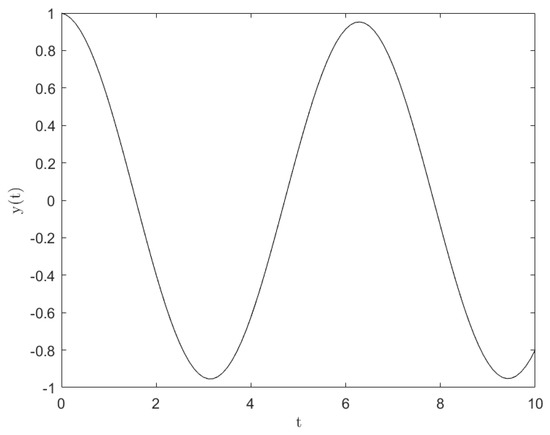
We refer to Figure 2. for the upper bound on the solution.

Figure 2. Using MATLAB, the graph shows the upper bound of this approximation at $t=0$ is 1.

4. Infinite Delay and Several Kernels

In this section, we extend the method to integral equations with infinite delay if the history of the solution is known and is a continuous function. Additionally, we generalize the concept to integral equations with several kernels.

We begin by considering scalar integral equations with infinite delay of the form

$$y\left(t\right)=b\left(t\right)-{\int }_{-\infty }^{t}C(t,s)g\left(y\left(s\right)\right)ds,$$

(24)

where b, C, and g are continuous. We assume the solution exists under some conditions. To specify a solution of (24), we require a continuous initial function $\phi :(-\infty ,0]\to \mathbb{R},$ with $\phi \left(0\right)=a\left(0\right),$ where

$$a\left(t\right):=b\left(t\right)-{\int }_{-\infty }^{0}C(t,s)g\left(\phi \left(s\right)\right)ds$$

is continuous so that

$$y\left(t\right)=a\left(t\right)-{\int }_0^{t}C(t,s)g\left(y\left(s\right)\right)ds,t\ge 0$$

(25)

is basically of the form of (15). With this set up, a function $y\left(t\right)$ is said to be a solution of (24), if $y\left(t\right)=\phi \left(t\right),$ for $t\le 0,$ and $y\left(t\right)$ satisfies (24) for $t\ge 0.$ Finally, Theorem 2 is exactly what would one needs to obtain boundedness results.

We end this paper with the extension to integral equations with N number of kernels and N number of nonlinear functions in $y.$ Thus, we consider the scalar nonlinear integral equation

$$y\left(t\right)=a\left(t\right)-{\int }_0^t\sum _{i=1}^N{C}_i(t,s)h_i\left(y\left(s\right)\right)ds,t\ge 0$$

(26)

where all functions are scalars and continuous on their respective domains. The functions $h_i,i=1\cdots N$ are continuous and satisfy the growth condition

$$|h_i\left(y\right)|\le {\lambda }_i\left|y\right|,i=1\cdots N$$

(27)

for positive constants ${\lambda }_i.$

Under this set up, the conditions of Lemmata 3 and 4 can be easily modified as seen next. Suppose there are differentiable functions ${\displaystyle {\psi }_i:[0,\infty )\to (0,\infty )}$ for $i=1,\cdots N,$ such that

$$\sum _{i=1}^N{\psi }_i^{\prime }(t-s)\le -\sum _{i=1}^N{\lambda }_i|C_i(t,s)|,0\le s\le t<\infty .$$

(28)

Moreover, if we assume the existence of a scalar function $\beta \left(t\right)$ that is uniformly continuous on $[0,\infty )$; then, we may redefine (21) as follows:

$${\int }_0^t\{\sum _{i=1}^N{\lambda }_i{\psi }_i(t-s)+\alpha \}\beta \left(s\right)ds=1.$$

(29)

If $y\left(t\right)$ is any solution of (26), then (18) is modified and given by

$$V\left(t\right)={\int }_0^t\sum _{i=1}^N{\lambda }_i{\psi }_i(t-s)\left|y\left(s\right)\right|ds,$$

(30)

Considering the above modifications, one can easily conclude the following theorem.

Theorem 3. 

Assume conditions (27), (28), and

$$\sum _{i=1}^N{\int }_0^{\infty }{\psi }_i\left(t\right)dt<\infty .$$

If $y\left(t\right)$ is any solution of (26), then

$$\left|y\left(t\right)\right|\le \frac{M}{\alpha },$$

where the constant $\alpha \in (0,1),$ such that

$$0<\sum _{i=1}^N{\lambda }_i{\psi }_i\left(0\right)<1\mathit{with}\alpha =1-\sum _{i=1}^N{\lambda }_i{\psi }_i\left(0\right),\mathit{and}M=\underset{t\ge 0}{max}\left|a\left(t\right)\right|.$$

Now, we offer an example.

Example 3. 

Consider the nonlinear integral equation

$$y\left(t\right)=t{e}^{-t}-{\int }_0^t\left[\frac{1}{{(t+2-s)}^3}sin\left(y\left(s\right)\right)+e^{-(t+3-s)}y\left(s\right)\right]ds.$$

(31)

Consequently, ${\displaystyle a\left(t\right)=t{e}^{-t},h\left(y\right)=sin\left(y\right),}$ and $C_1(t,s)=\frac{1}{{(t+2-s)}^3},C_2(t,s)=e^{-(t+3-s)}.$ Then, we have, ${\lambda }_1={\lambda }_2=1$ and $M=e^{-1}.$ Let ${\displaystyle {\psi }_1\left(t\right)=\frac{1}{{(t+2)}^2},{\psi }_2\left(t\right)=e^{-(t+3)}.}$ Then, it follows that

$${\int }_0^{\infty }{\psi }_i\left(t\right)dt<\infty ,i=1,2.$$

In addition, (28) is satisfied for $0\le s\le t<\infty .$ Moreover,

$$\alpha =1-{\lambda }_1{\psi }_1\left(0\right)-{\lambda }_2{\psi }_2\left(0\right))=1-\frac{1}{4}-e^{-3}=\frac{3}{4}-e^{-3}\in (0,1).$$

Thus, by Theorem 3 any solution $y\left(t\right)$ of (31) satisfies

$$\left|y\left(t\right)\right|\le \frac{M}{\alpha }=\frac{1/4}{3/4-e^{-3}}.$$

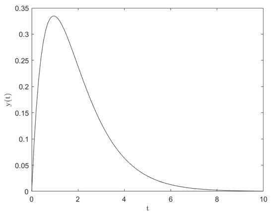
We refer to Figure 3. for the upper bound on the solution.

Figure 3. Using MATLAB, the graph shows the upper bound of this approximation is $0.3345$.

References

- Burton, T.A. Liapunov Functionals for Integral Equations; Trafford Publishing: Bloomington, IN, USA, 2008. [Google Scholar]
- Brauer, F.; Nohel, J.A. Qualitative Theory of Ordinary Differential Equations; Dover: New York, NY, USA, 1969. [Google Scholar]
- Coddington, E.A.; Levinson, N. Theory of Ordinary Differential Equations; McGraw-Hill Book Company: New York, NY, USA; London, UK, 1955. [Google Scholar]
- Cushing, J.M. Integro-Differential Equations and Delay Models in Population Dynamics; Lecture Notes in Biomathematics; Springer: Berlin, Germany; New York, NY, USA, 1977; Volume 20. [Google Scholar]
- Driver, R.D. Introduction to Ordinary Differential Equations; Harper & Row, Publishers: New York, NY, USA, 1978. [Google Scholar]
- Messina, E.; Raffoul, Y.N.; Vecchio, A. Qualitative Analysis of Dynamic Equations on Time Scales Using Lyapunov Functions. Differ. Equ. Appl. 2022, 14, 137–143. [Google Scholar] [CrossRef]
- Miller, R.K. Nonlinear Volterra Integral Equations; Benjamin: New York, NY, USA, 1971. [Google Scholar]
- Raffoul, Y. Advanced Differential Equations; Academic Press: Cambridge, MA, USA, 2023. [Google Scholar]
- Wang, M.; Saleem, N.; Bashir, S.; Zhou, M. Fixed point of modified F-Contraction with an application. Axioms 2022, 11, 413. [Google Scholar] [CrossRef]
- Alhamadi, F.; Raffoul, Y.N.; Alharbi, S. Boundedness and Stability of Solutions of Nonlinear Volterra Integro-Differential Equations. Adv. Dyn. Syst. Appl. 2018, 13, 19–31. [Google Scholar]
- Burton, T.A. Stability and Periodic Solutions of Ordinary and Functional Differential Equations; Academic Press: New York, NY, USA, 1985. [Google Scholar]
- Burton, T.A. Stability by Fixed Point Theory for Functional Differential Equations; Dover: New York, NY, USA, 2006. [Google Scholar]
- Islam, M.; Raffoul, Y. Bounded Solutions of Almost Linear Volterra Equation. Adv. Dyn. Syst. Appl. 2012, 7, 2. [Google Scholar]
- Tunc, C. New stability and boundedness results to Volterra integro-differential equations with delay. J. Egypt. Math. Soc. 2016, 24, 210–213. [Google Scholar] [CrossRef]
Disclaimer/Publisher’s Note: The statements, opinions and data contained in all publications are solely those of the individual author(s) and contributor(s) and not of MDPI and/or the editor(s). MDPI and/or the editor(s) disclaim responsibility for any injury to people or property resulting from any ideas, methods, instructions or products referred to in the content. |
© 2023 by the authors. Licensee MDPI, Basel, Switzerland. This article is an open access article distributed under the terms and conditions of the Creative Commons Attribution (CC BY) license (https://creativecommons.org/licenses/by/4.0/).