L₁-Norm Robust Regularized Extreme Learning Machine with Asymmetric C-Loss for Regression

Abstract

Extreme learning machines (ELMs) have recently attracted significant attention due to their fast training speeds and good prediction effect. However, ELMs ignore the inherent distribution of the original samples, and they are prone to overfitting, which fails at achieving good generalization performance. In this paper, based on expectile penalty and correntropy, an asymmetric C-loss function (called AC-loss) is proposed, which is non-convex, bounded, and relatively insensitive to noise. Further, a novel extreme learning machine called L₁ norm robust regularized extreme learning machine with asymmetric C-loss (L₁-ACELM) is presented to handle the overfitting problem. The proposed algorithm benefits from L₁ norm and replaces the square loss function with the AC-loss function. The L₁-ACELM can generate a more compact network with fewer hidden nodes and reduce the impact of noise. To evaluate the effectiveness of the proposed algorithm on noisy datasets, different levels of noise are added in numerical experiments. The results for different types of artificial and benchmark datasets demonstrate that L₁-ACELM achieves better generalization performance compared to other state-of-the-art algorithms, especially when noise exists in the datasets.

1. Introduction

The single hidden-layer feedforward neural network (SLFN) is one of the most important learning algorithms in data mining and machine learning fields. SLFN has only one hidden layer that connects the input and output layers. Generally, gradient-based algorithms are used to train SLFNs similar to back-propagation algorithms [1], which often leads to slow convergence, overfitting, and local minima. To overcome these problems, Huang et al. [2,3] proposed a widely used method based on the structure of SLFN called extreme learning machine (ELM). Compared to the traditional single hidden layer feedforward neural network, the input weights and thresholds of the hidden layer nodes in ELM are randomly generated, and there is no need for repeated adjustment via iterations. ELM identifies the output weight vector with the smallest norm by calculating the Moore-Penrose inverse. Therefore, the training speed of ELM is much higher than that of SLFN. Moreover, ELM also requires minimal training error and norm of the weights, which facilitates good generalization performance. Since ELM has a higher learning speed and better generalization performance, it has been successfully applied in many fields [4,5,6]. However, ELM still has several shortcomings. For example, ELM is based on empirical risk minimization (ERM) [7] which often leads to overfitting.

To address this issue, many scholars have proposed various algorithms based on ELM to improve the generalization performance. In [8], Deng et al. introduced the weight factor $\gamma$ into ELM for the first time and proposed the regularized extreme learning machine (RELM). By adjusting the weight factor $\gamma$, the proportion of empirical risk and structural risk in the actual prediction risk can be optimal, thereby avoiding model overfitting. However, RELM uses the L₂ norm which is sensitive to outliers. To reduce the influence of outliers, Rong et al. proposed the pruned extreme learning machine (P-ELM) [9], which can remove irrelevant hidden nodes. P-ELM is only used for classification problems. To further address the regression problem, the optimally pruned extreme learning machine (OP-ELM) [10] was proposed. In OP-ELM, The L₁ norm is used to remove irrelevant output nodes and select the corresponding hidden nodes, and then the weight of the corresponding hidden nodes is calculated using the least squares method. Given that the L₁ norm is robust to outliers, it is used in various algorithms to improve the generalization performance [11,12]. Balasundaram et al. [13] proposed the L₁ norm extreme learning machine, which produces sparse models such that decision functions can be determined using fewer hidden layer nodes. Generally speaking, RELM is composed of empirical risk and structural risk. Structural risk can effectively avoid overfitting, and structural risk is determined by loss function. Traditional RELMs use the squared loss function, which is symmetric and unbounded. The symmetry makes the model unable to take into account the distribution characteristics within the training samples, while unboundedness will cause the model to be sensitive to noise and outliers. In real life, the distribution of data is unbalanced, and noise is generally mixed in the process of data collection. Therefore, it is particularly important to choose an appropriate loss function to construct the model.

Quantiles can reflect completely the distribution of random variables without missing any information Quantile regression can more accurately describe the distribution characteristics of random variables for comprehensive analysis. Therefore, quantile regression is more robust and has been successfully applied to statistical prediction [14,15]. Quantile loss can be thought of as a pinball penalty. Expectile loss is an asymmetric least squares loss, which is the square of the quantile loss function. It is often used in regression problems with imbalanced data [16]. However, the unboundedness of the expectile loss leads to a lack of robustness.

From [17], the bounded loss function is less sensitive to noise and outliers than the unbounded loss function, whereas convex functions are usually unbounded. To further improve the robustness of ELM, researchers have proposed various non-convex loss functions to replace the convex loss functions [18,19,20]. Examples of common convex loss functions include square loss, hinge loss, and Huber loss, which allow for the determination of global optimal solutions and are easy to solve. However, the unboundedness of the convex loss function implies that it is not suited for handling outliers. Compared to convex loss functions, non-convex loss functions are more robust to outliers. Recently, Singh et al. [21] proposed a correntropy-based loss function called C-loss. Based on information theory and the kernel method, correntropy [22,23] is considered to be a generalized local similarity measure between two random variables. As a non-convex, bounded loss function, the C-loss function has been widely used in machine learning to improve robustness. In 2019, Zhao et al. [24] applied the C-loss function to ELM for the first time. They proposed the C-loss based ELM (CELM), and also experimentally demonstrated that the generalization performance was better compared to that of other algorithms.

In real life, the distribution of datasets tends to be asymmetric, and the training samples are easily contaminated by noise. In order to better consider the distribution characteristics inside the data and improve the generalization ability of the algorithm, a non-convex robust loss function is proposed, called asymmetric C-loss (AC-loss). A robust extreme learning machine based on the asymmetric C-loss and L₁-norm (called L₁-ACELM) is then developed. The main contributions of this report are as follows:

(1)

Based on the expectile penalty and correntropy loss function, a new loss function (AC-loss) is developed. AC-loss retains some important properties of C-loss such as non-convexity and boundedness. AC-loss is asymmetric, and it can handle unbalanced noise.

(2)

A novel approach called the L₁-norm robust regularized extreme learning machine with asymmetric C-loss (L₁-ACELM) is proposed by applying the proposed AC-loss function and the L₁-norm in the objective function of ELM to enhance robustness to outliers.

(3)

The non-convexity of the AC-loss function makes it difficult for L₁-ACELM to be solved. The half-quadratic optimization algorithm [25,26,27] is used to address these problems. Moreover, the convergence of the proposed algorithms is analyzed.

The remainder of this paper is structured as follows. Section 2 briefly reviews ELM, RELM, C-loss function, and the half-quadratic optimization algorithm. In Section 3, we propose the asymmetric C-loss function and the L₁-ACELM model. Next, the half-quadratic optimization algorithm is used to solve L₁-ACELM. In addition, we analyze the convergence of the algorithm. The experimental results for the artificial and benchmark datasets are presented in Section 4. Section 5 summarizes the main conclusions and further study.

2. Related Work

2.1. Extreme Learning Machine (ELM)

ELM is a new single hidden layer feedforward neural network that is first proposed by Huang et al. [2]. Unlike traditional SLFN, the input weights and thresholds of the hidden layer in ELM are randomly generated and the output weights can be determined using the least square method. Hence, it is much faster than traditional SLFN. In addition, ELM has good generalization ability.

Given $N$ arbitrary distinct samples $\left\{\mathit{X},\mathit{Y}\right\}={\left\{{\mathit{x}}_{\mathit{i}},{\mathit{y}}_{\mathit{i}}\right\}}_{\mathit{i}=1}^{\mathit{N}}$, ${\mathit{x}}_{\mathit{i}}={\left[x_{i1},x_{i2},\dots ,x_{im}\right]}^T\in {ℝ}^m$ and ${\mathit{y}}_{\mathit{i}}={\left[y_{i1},y_{i2},\dots ,y_{in}\right]}^T\in {ℝ}^n$ are the input samples and the corresponding output vectors, respectively. The output of a standard SLFN with L hidden nodes can be expressed as follows:

$$f\left(x_i\right)={\displaystyle \sum _{j=1}^L{\mathbf{\beta }}_{j}h\left({\mathbf{\alpha }}_j,b_j,x_i\right), i=1,\dots ,N}$$

(1)

where ${\mathbf{\alpha }}_j={\left[{\alpha }_{j1},{\alpha }_{j2},\dots ,{\alpha }_{jm}\right]}^T\in {ℝ}^m$ is the input weight vector that connects the input node to the j-th hidden layer node and $b_j\in R$ is the bias of the j-th hidden node. ${\mathbf{\beta }}_j={\left[{\beta }_{j1},{\beta }_{j2},\dots ,{\beta }_{jn}\right]}^T\in {ℝ}^n$ is the output weight vector that connects the j-th hidden layer node to the output node, and $h\left({\mathbf{\alpha }}_j,b_j,x_i\right)$ is the output of the j-th hidden layer node with respect to the input $x_i$. $f\left(\cdot \right)$ denotes the actual output vector of SLFN.

For ELM, the input weight vector and the bias that connects the input node to the hidden layer node are randomly assigned instead of being updated. Therefore, it can be converted to a linear model:

$$F=H\beta$$

(2)

where

$$H=\left[\begin{array}{c}h\left(x_1\right)\\ ⋮\\ h\left(x_N\right)\end{array}\right]={\left[\begin{array}{ccc}h\left({\alpha }_1,b_1,x_1\right)& \dots & h\left({\alpha }_L,b_L,x_1\right)\\ ⋮& \ddots & ⋮\\ h\left({\alpha }_1,b_1,x_N\right)& \dots & h\left({\alpha }_L,b_L,x_N\right)\end{array}\right]}_{N\times L}, \beta ={\left[\begin{array}{c}{\beta }_1^T\\ ⋮\\ {\beta }_L^T\end{array}\right]}_{L\times n} \mathrm{and} F={\left[\begin{array}{c}f{\left(x_1\right)}^T\\ ⋮\\ f{\left(x_N\right)}^T\end{array}\right]}_{N\times n}$$

Here, $H$ is the output matrix of the hidden layer. Thus, the output weight vector that connects the hidden layer node to the output node can be determined by solving the following equation:

$$\underset{\beta }{\min }{‖H\beta -Y‖}_2$$

(3)

ELM requires the approximation of the training samples with zero error. Therefore, Equation (3) can be written as:

$$H\beta =Y$$

(4)

The output weight $\beta$ is the least squares solution of Equation (4), which can be obtained as follows:

$$\beta =H^{+}Y$$

(5)

where $H^{+}$ is the Moore-Penrose generalized inverse of the matrix $H$.

To avoid overfitting of the model, regularized ELM is proposed, which facilitates better generalization performance by minimizing the sum of the training error and the norm of the output weights [28]. RELM can be expressed as follows:

$$\underset{\beta }{\min }{‖H\beta -Y‖}_2^2+\frac{\gamma }{2}{‖\beta ‖}_2^2$$

(6)

The optimal solution to RELM is computed as follows:

$$\beta =\left\{\begin{array}{c}{\left(H^{T}H+\gamma I\right)}^{-1}{H}^{T}Y if N\ge L\\ H^T{\left(H{H}^T+\gamma I\right)}^{-1}Y if N<L\end{array}\right.$$

(7)

where $I$ is an identity matrix.

2.2. Correntropy-Induced Loss (C-Loss)

Correntropy is a generalized similarity measure between two random variables in a small neighborhood defined by the kernel width $\sigma$. For a regression problem, the choice of the loss function could ensure that the similarity between the actual output and the target value is maximized, which is equivalent to the maximization of correntropy. Thus, the C-loss function [21] is proposed by Singh et al., which is defined as:

$$L_C\left(y_i,f\left(x_i\right)\right)=1-\exp \left\{-\frac{{\left(y_i-f\left(x_i\right)\right)}^2}{2{\sigma }^2}\right\}$$

(8)

As a bounded non-convex loss function, the C-loss loss function is more robust to outliers than the traditional squared loss function.

2.3. Half-Quadratic Optimization

The half-quadratic optimization algorithm based on the conjugate function theory [29] is usually used for convex optimization and non-convex optimization problems. This method transforms the original non-convex objective function into a half-quadratic objective function by introducing auxiliary variables. As such, the objective function cannot be solved directly, and a two-step alternating minimization method is required. The specific operations are as follows: given the original variables, the auxiliary variables are optimized. The variables are then optimized, and the original variables are determined.

The minimization problem is as follows:

$$\underset{v}{\min }{\varphi }_v\left(v\right)+F\left(v\right)$$

(9)

where $v={\left[v_1,v_2,\dots ,v_N\right]}^T\in {ℝ}^N$, $\varphi \left(\cdot \right)$ is a potential loss function with $\varphi \left(v\right)={\displaystyle \sum _{i=1}^N\varphi \left(v_i\right)}$ and $F\left(\cdot \right)$ is a convex penalty function.

Considering the half-quadratic optimization algorithm, we introduce an auxiliary variable $p={\left[p_1,p_2,\dots ,p_N\right]}^T\in {ℝ}^N$ into $\varphi \left(\cdot \right)$, which can then be expressed as:

$$\varphi \left(v_i\right)=\underset{p_i}{\min }\left\{Q\left(v_i,p_i\right)+\phi \left(p_i\right)\right\}$$

(10)

where $Q\left(v_i,p_i\right)$ is a half-quadratic function, which can be represented in the additive form $Q_A\left(v_i,p_i\right)=\frac{1}{2}{\left(\sqrt{c}{v}_i-p_i/\sqrt{c}\right)}^2$ or the multiplicative form $Q_M\left(v_i,p_i\right)=\frac{1}{2}{p}_i{v}_i{}^2$.

Substituting Equation (10) into Equation (9), we obtain the following optimization problem:

$$\underset{v}{\min }{\varphi }_v\left(v\right)+F\left(v\right)=\underset{v,p}{\min }\left\{Q\left(v,p\right)+\phi \left(p\right)+F\left(v\right)\right\}$$

(11)

where $p_i$ is determined using a function $g\left(\cdot \right)$, which is the conjugate function of $\varphi \left(\cdot \right)$. Alternatively, Equation (11) can then be optimized as follows:

$$p^{t+1}=g\left(v\right)$$

(12)

$$v^{t+1}=\underset{v}{\arg \min }\left\{Q\left(v,p^{t+1}\right)+F\left(v\right)\right\}$$

(13)

where t represents the t-th iteration.

3. Main Contributions

3.1. Asymmetric C-Loss Function (AC-Loss)

As a measure of risk, the expectile is an extension of the quantile, which represents the distributional information of a random variable. The expectile loss is essentially a squared pinball loss, which can also be considered as an asymmetric squared loss. The asymmetric least square loss function can be expressed as:

$$L_{\tau }\left(y_i,f\left(x_i\right)\right)=\left\{\begin{array}{c}\tau {\left(y_i-f\left(x_i\right)\right)}^2\\ \left(1-\tau \right){\left(y_i-f\left(x_i\right)\right)}^2\end{array}\right.\begin{array}{c}if y_i-f\left(x_i\right)\ge 0\\ if y_i-f\left(x_i\right)<0\end{array}$$

(14)

However, given that the asymmetric least square loss is an unbounded loss function, it is more sensitive to outliers. Therefore, we construct an asymmetric C-loss (AC-loss) function, based on the C-loss function and the expectile loss function, which is a non-convex, asymmetric, and bounded function for dealing with outliers and noise. The AC-loss function is defined as follows:

$$L_C^{als}\left(y_i,f\left(x_i\right)\right)=\left\{\begin{array}{cc}1-\exp \left\{\frac{-\tau {\left(y_i-f\left(x_i\right)\right)}^2}{2{\sigma }^2}\right\}& if y_i-f\left(x_i\right)\ge 0\\ 1-\exp \left\{\frac{-\left(1-\tau \right){\left(y_i-f\left(x_i\right)\right)}^2}{2{\sigma }^2}\right\}& if y_i-f\left(x_i\right)<0 \end{array}\right.$$

(15)

The plot of the AC-loss function is shown in Figure 1.

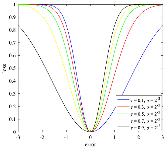
Figure 1. Asymmetric C-loss function.

3.2. L₁-ACELM

To improve the generalization performance of RELM, the proposed loss function is introduced to replace the squared loss function. To further enhance robustness to outliers, the L₂ norm of structural risk in RELM is replaced with the L₁ norm. Therefore, we propose a new robust ELM (called L₁-ACELM):

$$\underset{\beta }{\min } J\left(\beta \right)={\displaystyle \sum _{i=1}^N{L}_C^{als}\left(y_i-h\left(x_i\right)\beta \right)}+\gamma {‖\beta ‖}_1$$

(16)

where $\gamma >0$ is a regularized parameter.

Since AC-loss is a non-convex loss function, it is difficult to directly optimize the objective function. The half-quadratic optimization algorithm is usually applied to optimize non-convex problems. Therefore, we chose the half-quadratic optimization algorithm to find the optimal solution of the objective function.

3.3. Solving Method

For the function $f\left(u\right)=\exp \left(u\right)$, there exists a convex function $g\left(v\right)$, which is expressed as follows:

$$g\left(v\right)=-v\log \left(-v\right)+v$$

(17)

where $v<0$, and the conjugate function $g^{\ast }\left(u\right)$ of the function $g\left(v\right)$ is defined as:

$$g^{\ast }\left(u\right)=\underset{v}{\sup }\left\{uv+v\log \left(-v\right)-v\right\}$$

(18)

where

$$v=-\exp \left(-u\right)<0$$

(19)

By substituting Equation (19) into Equation (18), we have

$$g^{\ast }\left(u\right)=\exp \left(-u\right)$$

(20)

Now, let $u=\left\{\begin{array}{cc}\frac{\tau e_i^2}{2{\sigma }^2}& if e_i\ge 0\\ \frac{\left(1-\tau \right)e_i^2}{2{\sigma }^2}& if e_i<0 \end{array}\right.$ and $e_i=y_i-h\left(x_i\right)\beta$, then Equation (18) can be expressed as:

$$g^{\ast }\left(u\right)=\left\{\begin{array}{c}\underset{v}{\sup }\left\{\frac{\tau e_i^2}{2{\sigma }^2}v+v\log \left(-v\right)-v\right\}\\ \underset{v}{\sup }\left\{\frac{\left(1-\tau \right)e_i^2}{2{\sigma }^2}v+v\log \left(-v\right)-v\right\}\end{array}\right.=\left\{\begin{array}{cc}\exp \left(-\frac{\tau e_i^2}{2{\sigma }^2}\right)& if e_i\ge 0\\ \exp \left(-\frac{\left(1-\tau \right)e_i^2}{2{\sigma }^2}\right)& if e_i<0 \end{array}\right.$$

(21)

where

$$v_i=\left\{\begin{array}{cc}-\exp \left(-\frac{\tau e_i^2}{2{\sigma }^2}\right)& if e_i\ge 0\\ -\exp \left(-\frac{\left(1-\tau \right)e_i^2}{2{\sigma }^2}\right)& if e_i<0 \end{array}\right.$$

(22)

By combining Equations (21) and (16), we have

$$\begin{array}{l}\underset{\beta ,v}{\min } J\left(\beta ,v\right)=\left\{\begin{array}{cc}{\displaystyle \sum _{i=1}^N\left(1-\underset{v_i}{\sup }\left\{\exp \left(-\frac{\tau e_i^2}{2{\sigma }^2}\right)v_i+g\left(v_i\right)\right\}\right)}+\gamma {‖\beta ‖}_1& if e_i\ge 0\\ {\displaystyle \sum _{i=1}^N\left(1-\underset{v_i}{\sup }\left\{\exp \left(-\frac{\left(1-\tau \right)e_i^2}{2{\sigma }^2}\right)v_i+g\left(v_i\right)\right\}\right)}+\gamma {‖\beta ‖}_1& if e_i<0 \end{array}\right.\\ s.t. \beta h\left(x_i\right)=y_i-e_i,i=1,2,\dots ,N\end{array}$$

(23)

where $v={\left[v_1,v_2,\dots ,v_N\right]}^T$. Equation (23) can be simplified as:

$$\begin{array}{l}\underset{\beta ,v}{\min } J^{\prime }\left(\beta ,v\right)=\left\{\begin{array}{cc}\underset{v}{\sup }\left\{{\displaystyle \sum _{i=1}^N\left(-\frac{\tau e_i^2}{2{\sigma }^2}{v}_i-v_i\log \left(-v_i\right)+v_i\right)}\right\}+\gamma {‖\beta ‖}_1& if e_i\ge 0\\ \underset{v}{\sup }\left\{{\displaystyle \sum _{i=1}^N\left(-\frac{\left(1-\tau \right)e_i^2}{2{\sigma }^2}{v}_i-v_i\log \left(-v_i\right)+v_i\right)}\right\}+\gamma {‖\beta ‖}_1& if e_i<0 \end{array}\right.\\ s.t. h\left(x_i\right)\beta =y_i-e_i, i=1,2,\dots ,N\end{array}$$

(24)

The optimal solution $\beta$ can be obtained by solving Equation (24) using the alternating optimization method.

Firstly, given the original variables ${\beta }^t$, we can obtain the optimal solution for the auxiliary variables $v^{t+1}$. When ${\beta }^t$ is given, the minimization problem is given as follows:

$$\underset{v}{\min } J\left(v\right)=\left\{\begin{array}{cc}{\displaystyle \sum _{i=1}^N\left(-\frac{\tau {\left(y_i-f\left(x_i\right)\right)}^2}{2{\sigma }^2}{v}_i-v_i\log \left(-v_i\right)+v_i\right)}& if e_i\ge 0\\ {\displaystyle \sum _{i=1}^N\left(-\frac{\left(1-\tau \right){\left(y_i-f\left(x_i\right)\right)}^2}{2{\sigma }^2}{v}_i-v_i\log \left(-v_i\right)+v_i\right)}& if e_i<0 \end{array}\right.$$

(25)

According to the half-quadratic optimization algorithm, the auxiliary variables $v^{t+1}$ can be obtained by solving Equation (24). Thus, we have:

$$v_i^{t+1}=\left\{\begin{array}{cc}-\exp \left(-\frac{\tau {\left(y_i-f^t\left(x_i\right)\right)}^2}{2{\sigma }^2}\right)& if e_i\ge 0\\ -\exp \left(-\frac{\left(1-\tau \right){\left(y_i-f^t\left(x_i\right)\right)}^2}{2{\sigma }^2}\right)& if e_i<0 \end{array}\right.,i=1,2,\dots ,N$$

(26)

Secondly, the auxiliary variables $v^{t+1}$ are fixed and the optimal solution of the original variable ${\beta }^{t+1}$ can be obtained by solving the following minimization problem:

$$\begin{array}{l}\underset{{\beta }^{t+1}}{\min } J\left({\beta }^{t+1}\right)=\left\{\begin{array}{cc}{\displaystyle \sum _{i=1}^N\left(-\frac{\tau v_i}{2{\sigma }^2}{e}_i^2\right)}+\gamma {‖{\beta }^{t+1}‖}_1& if e_i\ge 0\\ {\displaystyle \sum _{i=1}^N\left(-\frac{\left(1-\tau \right)v_i}{2{\sigma }^2}{e}_i^2\right)}+\gamma {‖{\beta }^{t+1}‖}_1& if e_i<0 \end{array}\right.\\ s.t. {\beta }^{t+1}h\left(x_i\right)=y_i-e_i,i=1,2,\dots ,N\end{array}$$

(27)

Equation (27) is equivalent to

$$\underset{{\beta }^{t+1}}{\min } J\left({\beta }^{t+1}\right)=\left\{\begin{array}{ll}{\displaystyle \sum _{i=1}^N\left(-\frac{\tau v_i^{t+1}}{2{\sigma }^2}{\left(y_i-h\left(x_i\right){\beta }^{t+1}\right)}^2\right)}+\gamma {‖{\beta }^{t+1}‖}_1\hfill & if y_i\ge h\left(x_i\right){\beta }^{t+1}\\ {\displaystyle \sum _{i=1}^N\left(-\frac{\left(1-\tau \right)v_i^{t+1}}{2{\sigma }^2}{\left(y_i-h\left(x_i\right){\beta }^{t+1}\right)}^2\right)}+\gamma {‖{\beta }^{t+1}‖}_1 \hfill & if y_i<h\left(x_i\right){\beta }^{t+1}\end{array}\right.$$

(28)

Since the L₁ norm exists in the objective function, the proximal gradient descent (PGD) algorithm is applied to solve the optimization problem Equation (28). The objective function $J\left({\beta }^{t+1}\right)$ can be written as

$$J\left({\beta }^{t+1}\right)=S\left({\beta }^{t+1}\right)+\gamma {‖{\beta }^{t+1}‖}_1,$$

(29)

where

$$S\left({\beta }^{t+1}\right)=\left\{\begin{array}{ll}{\displaystyle \sum _{i=1}^N\left(-\frac{\tau v_i^{t+1}}{2{\sigma }^2}{\left(y_i-h\left(x_i\right){\beta }^{t+1}\right)}^2\right)}\hfill & if y_i\ge h\left(x_i\right){\beta }^{t+1}\\ {\displaystyle \sum _{i=1}^N\left(-\frac{\left(1-\tau \right)v_i^{t+1}}{2{\sigma }^2}{\left(y_i-h\left(x_i\right){\beta }^{t+1}\right)}^2\right)}\hfill & if y_i<h\left(x_i\right){\beta }^{t+1}\end{array}\right.$$

(30)

$S\left({\beta }^{t+1}\right)$ is differentiable and its derivative is as follows:

$$\nabla S\left({\beta }^{t+1}\right)=\left\{\begin{array}{ll}{\displaystyle \sum _{i=1}^N\left(\frac{\tau v_i^{t+1}}{{\sigma }^2}{h}^T\left(x_i\right)\left(y_i-h\left(x_i\right){\beta }^{t+1}\right)\right)}\hfill & if y_i\ge h\left(x_i\right){\beta }^{t+1}\\ {\displaystyle \sum _{i=1}^N\left(\frac{\left(1-\tau \right)v_i^{t+1}}{{\sigma }^2}{h}^T\left(x_i\right)\left(y_i-h\left(x_i\right){\beta }^{t+1}\right)\right)}\hfill & if y_i<h\left(x_i\right){\beta }^{t+1}\end{array}\right.$$

(31)

Since $\nabla S\left({\beta }^{t+1}\right)$ satisfies the L-Lipschitz continuity condition, there is a constant $\eta >0$ such that

$${‖\nabla S\left(\beta \right)-\nabla S\left({\beta }^{t+1}\right)‖}_2^2\le \eta {‖\beta -{\beta }^{t+1}‖}_2^2,\forall \left(\beta ,{\beta }^{t+1}\right)$$

(32)

The second-order Taylor expansion of the function $S\left({\beta }^{t+1}\right)$ can be expressed as

$$\begin{array}{ll}S\left(\beta ;{\beta }^{t+1}\right)& \approx S\left({\beta }^{k+1}\right)+\nabla S\left({\beta }^{k+1}\right)\left(\beta -{\beta }^{k+1}\right)+\frac{\eta }{2}‖\beta -{\beta }^{k+1}‖\\ & =\frac{\eta }{2}{‖\beta -\left({\beta }^{k+1}-\frac{1}{\eta }\nabla S\left({\beta }^{k+1}\right)\right)‖}_2^2+\delta \left({\beta }^{k+1}\right)\end{array}$$

(33)

where $\delta \left({\beta }^{t+1}\right)$ is a constant that is independent of ${\beta }^{t+1}$.

Introducing ${‖{\beta }^{t+1}‖}_1$ into the objective function, the iterative equation of the proximal gradient descent can be expressed as

$${\beta }^{t+1}=\underset{{\beta }^{t+1}}{\arg \min }\frac{\eta }{2}{‖\beta -\left({\beta }^{t+1}-\frac{1}{\eta }\nabla S\left({\beta }^{t+1}\right)\right)‖}_2^2+\gamma {‖{\beta }^{t+1}‖}_1$$

(34)

Let $z={\beta }^{t+1}-\frac{1}{\eta }\nabla S\left({\beta }^{t+1}\right)$. Then, the closed-form solution of Equation (34) can be written as:

$${\beta }_i^{{}^{t+1}}=\left\{\begin{array}{cc}{z}_i-\gamma /\eta & \gamma /\eta <z_i\\ 0& \left|z_i\right|\le \gamma /\eta \\ z_i+\gamma /\eta & z_i<-\gamma /\eta \end{array}\right.,i=1,2,\dots ,N$$

(35)

where ${\beta }_i^{{}^{t+1}}$ and $z_i$ represent the i-th component of ${\beta }^{t+1}$ and $z$, respectively. We develop a half-quadratic optimization to solve the proposed model, and the pseudo code is presented in Algorithm 1.

Algorithm 1. Half-quadratic optimization for L1-ACELM

Input: The training dataset $T={\{(x_i,y_i)\}}_{i=1}^N$, the number of hidden layer nodes L, the activation function $h\left(x\right)$, the regularization parameter $\gamma$, the maximum number of iterations $t_{\max }$, window width $\sigma$, a small number $\rho$ and the parameter $\tau$. Output: the output weight vector $\beta$. Step 1. Randomly generate input weight ${\alpha }_i$ and hidden layer bias $b_i$ with L hidden nodes. Step 2. Calculate hidden output matrix $H\left(x\right)$. Step 3. Compute $\beta$ by Equation (7). Step 4. Let ${\beta }^0=\beta$ and ${\beta }^1=\beta$, set $t=1$. Step 5. While $\left|J\left({\beta }^t\right)-J\left({\beta }^{t-1}\right)\right|<\rho$ or $t<t_{\max }$ do calculate $v_i^{t+1}$ by Equation (26). update ${\beta }^{t+1}$ using Equation (35). compute $J\left({\beta }^{t+1}\right)$ by Equation (29). update t: = t + 1. End while Step 6: Output result given by $\beta ={\beta }^{t-1}$.

3.4. Convergence Analysis

Proposition 1.

The sequence$\left\{J\left({\beta }^t,v^t\right),t=1,2,\dots ,t\right\}$generated by Algorithm 1 is convergent.

Proof. 

Let ${\beta }^t$ and $v^t$ be the optimal solution to the objective function (23) after t iterations. In the half-quadratic optimization problem, the conjugate function $g^{\ast }\left(\cdot \right)$ satisfies $\left\{Q\left({\beta }_i,g^{\ast }\left({\beta }_i\right)\right)+\phi \left({\beta }_i\right)\right\}\le \left\{Q\left({\beta }_i,g^{\ast }\left(v_i\right)\right)+\phi \left(v_i\right)\right\}$. When ${\beta }^t$ is fixed, we can obtain the optimal solution $v^{t+1}$ of $v$ at the (t + 1)-th iteration from Equation (26), then we have:

$$J\left({\beta }^t,v^{t+1}\right)\le J\left({\beta }^t,v^t\right)$$

(36)

Next, when $v^{t+1}$ is fixed, we can optimize (28) to obtain the solution ${\beta }^{t+1}$ of $\beta$ at the (t + 1)-th iteration. Then we have:

$$J\left({\beta }^{t+1},v^{t+1}\right)\le J\left({\beta }^t,v^{t+1}\right)$$

(37)

Combining Inequation (36) with Inequality (37), we have:

$$J\left({\beta }^{t+1},v^{t+1}\right)\le J\left({\beta }^t,v^{t+1}\right)\le J\left({\beta }^t,v^t\right)$$

(38)

Hence, the optimization problem $J\left(\beta ,v\right)$ is bounded, and the sequence $\left\{J\left({\beta }^t,v^t\right),t=1,2,\dots ,t\right\}$ is convergent. □

4. Experiments

4.1. Experimental Setup

To evaluate the performance of the proposed L₁-ACELM algorithm, we performed numerical simulations using two artificial datasets and ten standard benchmark datasets. To show the effectiveness of the L₁-ACELM algorithm compared to traditional algorithms including extreme learning machine (ELM), regularized ELM (RELM), and C-loss based ELM (CELM), several experiments were performed. All experiments were implemented in Matlab2016a on a PC with an i5-7200U Intel(R) Core (TM) processor (2.70 GHz) 4 GB RAM.

To evaluate the prediction performance of the L₁-ACELM algorithm, the regression evaluation metrics are defined as follows:

(1)

The root mean square error (RMSE)

$$RMSE=\sqrt{\frac{1}{N}{\displaystyle \sum _{i=1}^N{\left(y_i-{\widehat{y}}_i\right)}^2}}$$

(39)

(2)

Mean absolute error (MAE)

$$MAE=\frac{1}{N}{\displaystyle \sum _{i=1}^N\left|y_i-{\widehat{y}}_i\right|}$$

(40)

(3)

The ratio of the sum squared error (SSE) to the sum squared deviation of the sample SST (SSE/SST) is given as:

$$SSE/SST=\frac{{\displaystyle \sum _{i=1}^N{\left({\widehat{y}}_i-y_i\right)}^2}}{{\displaystyle \sum _{i=1}^N{\left(y_i-{\overline{y}}_i\right)}^2}}$$

(41)

(4)

The ratio between the interpretable sum deviation SSR and SST (SSR/SST) is given by:

$$SSR/SST=\frac{{\displaystyle \sum _{i=1}^N{\left({\widehat{y}}_i-{\overline{y}}_i\right)}^2}}{{\displaystyle \sum _{i=1}^N{\left(y_i-{\overline{y}}_i\right)}^2}}$$

(42)

where $N$ is the number of samples. $y_i$ and ${\widehat{y}}_i$ denote the target values and the corresponding predicted values, respectively. ${\overline{y}}_i$ can be calculated from ${\overline{y}}_i=\frac{1}{N}{\displaystyle \sum _{i=1}^N{y}_i}$, which represents the average value of $y_1,y_2,\dots ,y_N$. The sigmoid function is chosen as the activation function for ELM, RELM, CELM, and L₁-ACELM, and can be expressed as:

$$h\left(x\right)=\frac{1}{1+\exp \left(-a_i^{T}x+b_i\right)}$$

(43)

Since the original algorithms and the proposed algorithm involve many parameters, to ensure the best performance, ten-fold cross-validation is used to determine the optimal parameters. In ELM and RELM, the number of hidden layer nodes $L=30$ is fixed. For RELM, CELM, and L₁-ACELM, the optimal value of the regularization parameter $\gamma$ is selected from the set {2⁻⁵⁰, 2⁻⁴⁹, …, 2⁴⁹, 2⁵⁰}. For CELM and L₁-ACELM, the window width $\sigma$ is selected from the range {2⁻², 2⁻¹, 2⁰, 2¹, 2²}. For L₁-ACELM, the parameter $\tau$ is obtained from the set {0.1, 0.2, …, 0.9}.

4.2. Performance on Artificial Datasets

To verify the robustness of the proposed L₁-ACELM, two artificial datasets were generated using six different types of noise, both of which consisted of 2000 data points. Table 1 shows the specific forms of two artificial datasets and different types of noise. ${\lambda }_i\sim N\left(0,s^2\right)$ indicates that ${\lambda }_i$ has a normal distribution with a mean of zero and variance of $s^2$, ${\lambda }_i\sim U\left(a,b\right)$ means that ${\lambda }_i$ has a uniform distribution in the interval $[a,b]$, ${\lambda }_i\sim T\left(c\right)$ indicates that ${\lambda }_i$ has a t-distribution with $c$ degrees of freedom.

Table 1. Artificial datasets with different types of noise.

Artificial Dataset	Function Definition	Types of Noise
Sinc function	$y_i=\sin c\left(2x_i\right)=\frac{\sin \left(2x_i\right)}{2x_i}+{\lambda }_i$	Type A: $x\in \left[-3,3\right]$,${\lambda }_i\sim N\left(0,0.15^2\right)$ Type B: $x\in \left[-3,3\right]$,${\lambda }_i\sim N\left(0,0.5^2\right)$ Type C: $x\in \left[-3,3\right]$,${\lambda }_i\sim U\left(-0.15,0.15\right)$ Type D: $x\in \left[-3,3\right]$,${\lambda }_i\sim U\left(0.5,0.5\right)$ Type E: $x\in \left[-3,3\right]$,${\lambda }_i\sim T\left(5\right)$ Type F: $x\in \left[-3,3\right]$,${\lambda }_i\sim T\left(10\right)$
Self-defining function	$y_i=e^{x_i^2\sin c\left(0.3\pi x_i\right)}+{\lambda }_i$

Figure 2 shows different types of noise graphs, the graphs of the sinc function, and the graphs of the sinc function with different noises.

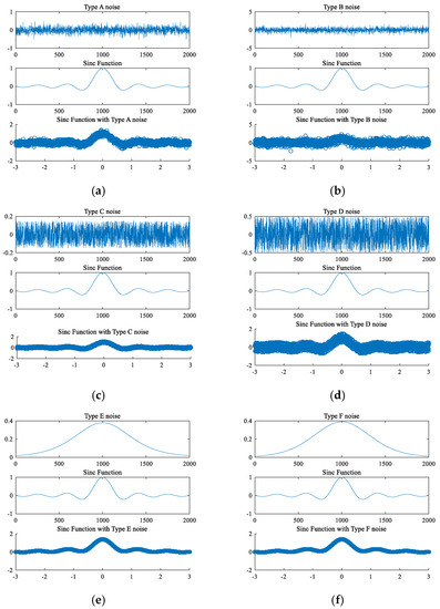
Figure 2. Graphs of the sinc function with different noises.

Figure 3 shows different types of noise graphs, the graphs of the self-defining function, and the graphs of the self-defining function with different noises.

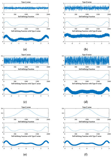
Figure 3. Graphs of the self-defining function with different noises.

In our experiments, we randomly selected 1600 samples as the training dataset and the remaining 400 samples as the testing dataset. To evaluate the effectiveness of the proposed algorithm, we compared its performance to that of ELM, RELM, and CELM. Table 2 shows the optimal RMSE, MAE, SSE/SST, and SSR/SST of the four algorithms that were obtained based on the optimal parameters selected using the ten-fold cross-validation method. Table 2 also lists the optimal parameters for each algorithm. The regression fitting results of ELM, RELM, CELM, and L₁-ACELM on two artificial datasets with noise are shown in Figure 4 and Figure 5.

Table 2. Experiment results on artificial datasets with different types of noise.

Dataset	Noise	Algorithm	$(\mathit{\gamma },\mathit{\sigma },\mathit{\tau })$	RMSE	MAE	SSE/SST	SSR/SST
Sinc function	Type A	ELM RELM CELM L1−ACELM	(/, /, /) (220, /, /) (210, 2−2, /) (2−23, 2−2, 0.7)	0.2429 0.2341 0.2345 0.2109	0.1957 0.1942 0.1949 0.1690	0.6206 0.5768 0.5785 0.4680	0.3808 0.4263 0.4256 0.5359
	Type B	ELM RELM CELM L1−ACELM	(/, /, /) (22, /, /) (2−19, 2−2, /) (25, 2−2, 0.3)	0.5288 0.5270 0.5286 0.5221	0.4199 0.4186 0.4199 0.4143	0.9064 0.9004 0.9060 0.8838	0.0988 0.1004 0.0991 0.1246
	Type C	ELM RELM CELM L1−ACELM	(/, /, /) (2−42, /, /) (210, 2−2, /) (239, 2−2, 0.7)	0.1923 0.2019 0.1922 0.1595	0.1581 0.1677 0.1582 0.1309	0.4332 0.4776 0.4325 0.2978	0.5701 0.5233 0.5705 0.7023
	Type D	ELM RELM CELM L1−ACELM	(/, /, /) (212, /, /) (2−38, 2−2, /) (2−4, 2−2, 0.3)	0.3262 0.3246 0.3223 0.3199	0.2715 0.2709 0.2695 0.2678	0.6963 0.6890 0.6828 0.6706	0.7633 0.7578 0.7664 0.8571
	Type E	ELM RELM CELM L1−ACELM	(/, /, /) (212, /, /) (2−12, 2−2, /) (2−12, 2−2, 0.2)	0.1737 0.1766 0.1725 0.1349	0.1406 0.1441 0.1398 0.1175	0.2369 0.2451 0.2338 0.1431	0.7633 0.7578 0.7664 0.8571
	Type F	ELM RELM CELM L1−ACELM	(/, /, /) (2−2, /, /) (2−1, 2−2, /) (2−3, 2−2, 0.1)	0.1885 0.1746 0.1757 0.1753	0.1422 0.1412 0.1413 0.1416	0.2715 0.2328 0.2359 0.2346	0.7298 0.7681 0.7651 0.7663
	Type A	ELM RELM CELM L1−ACELM	(/, /, /) (2−8, /, /) (2−7, 2−2, /) (2−10, 2−2, 0.5)	0.1572 0.1569 0.1565 0.1560	0.1304 0.1301 0.1294 0.1241	0.0908 0.0893 0.0888 0.0800	0.9105 0.9120 0.9127 0.9211
	Type B	ELM RELM CELM L1−ACELM	(/, /, /) (226, /, /) (215, 2−2, /) (2−16, 2−2, 0.2)	0.4905 0.4862 0.4858 0.4849	0.3843 0.3850 0.3838 0.3795	0.4761 0.4766 0.4759 0.4641	0.5251 0.5249 0.5252 0.5369
	Type C	ELM RELM CELM L1−ACELM	(/, /, /) (225, /, /) (217, 2−2, /) (237, 2−2, 0.2)	0.0937 0.0950 0.0936 0.0934	0.0794 0.0803 0.0792 0.0791	0.0288 0.0296 0.0287 0.0286	0.9714 0.9706 0.9715 0.9716
	Type D	ELM RELM CELM L1−ACELM	(/, /, /) (215, /, /) (2−34, 2−2, /) (222, 2−2, 0.7)	0.3009 0.3006 0.2948 0.2929	0.2622 0.2614 0.2555 0.2534	0.2471 0.2466 0.2373 0.2342	0.7534 0.7539 0.7634 0.7665
	Type E	ELM RELM CELM L1−ACELM	(/, /, /) (2−26, /, /) (22, 2−2, /) (244, 2−2, 0.4)	0.0434 0.0426 0.0425 0.0415	0.0372 0.0367 0.0363 0.0335	0.0074 0.0071 0.0071 0.0068	0.9929 0.9932 0.9932 0.9935
Self−defining function	Type F	ELM RELM CELM L1−ACELM	(/, /, /) (25, /, /) (212, 2−2, /) (220, 2−2, 0.3)	0.0498 0.0761 0.0481 0.0513	0.0425 0.0586 0.0408 0.0372	0.0098 0.0230 0.0092 0.0104	0.9912 0.9779 0.9920 0.9908

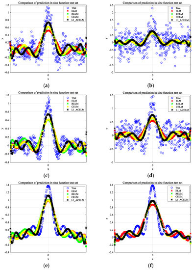
Figure 4. Fitting results of the sinc function with different noises.

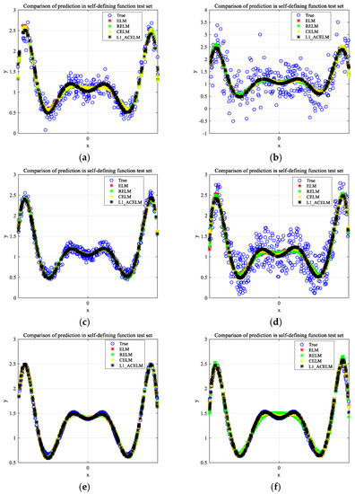
Figure 5. Fitting results of the self-defining function with different noises.

Figure 4 and Figure 5 demonstrate the fitting effect of the four algorithms on the two artificial datasets. Based on these figures, it is observed that the fitting curve of L₁-ACELM is the closest to the real function curve compared to the other three algorithms. In Table 2, the best test results are shown in bold.

The data in Table 2 demonstrate that L₁-ACELM exhibits better performance in most cases when compared to the other three algorithms for the two artificial datasets with different noises. It is evident that L₁-ACELM has smaller RMSE, MAE, and SSE/SST, and larger SSE/SSR. This indicates that L₁-ACELM is more robust to noise. For example, for the sinc function, except for F noise, the performance of the proposed algorithm is superior to that of the other algorithms for different types of noise. Moreover, it is seen that L₁-ACELM has better generalization performance in the case of unbalanced noise data. In conclusion, L₁-ACELM is more stable in a noisy environment.

4.3. Performance on Benchmark Datasets

To further test the robustness of L₁-ACELM, experiments were performed on ten UCI datasets [30] with different levels of noise, including noise-free datasets, datasets with 5% noise, and datasets with 10% noise. Noise datasets were only added to the target output value of the training datasets. Among them, datasets with 5% noise indicate that the noisy data are 5% of the training dataset. The data in the noisy dataset are randomly taken from the set $[0,d]$, where d is the average of the target output values of the training datasets.

In the experiment, we randomly selected 80% of the data as the training dataset and the remaining 20% as the testing dataset for each benchmark dataset. The specific description is shown in Table 3.

Table 3. Description of benchmark datasets.

Dataset	Number of Training Data	Number of Testing Data	Number of Features
Boston Housing	404	102	13
Air Quality	7485	1872	12
AutoMPG	313	79	7
Triazines	148	38	60
Bodyfat	201	51	14
Pyrim	59	15	27
Servo	133	34	4
Bike Sharing	584	147	13
Balloon	1600	401	1
NO2	400	100	7

To better reflect the performance of the proposed algorithm L₁-ACELM, the RMSE, MAE, SSE/SST, and SSR/SST were compared with those of ELM, RELM, and CELM. The evaluation indicators and the ranking of each algorithm for different noise environments are listed in Table 4, Table 5 and Table 6, and the best test results are shown in bold. From Table 4 to Table 6, it is observed that the performance of each algorithm decreases as the noise level increases. However, compared to the other algorithms, the performance of L₁-ACELM is still the best in most cases. From Table 4, it can be concluded that L₁-ACELM performs best on nine datasets out of a total of ten datasets in term of the RMSE and SSR/SST values. Similarly, for the MAE and SSE/SST values, L₁-ACELM exhibits the best performance on all the datasets. Table 5 shows that after adding 5% noise, the performance of each algorithm decreases, and according to the RMSE value, the proposed algorithm performed well on eight of the ten datasets. For the MAE, SSE/SST, and SSR/SST values, L₁-ACELM performs better for nine datasets. Moreover, for the RMSE, MAE, and SSR/SST values, it exhibits superior performance in nine cases and for the SSE/SST values, it has better performance in all ten datasets.

Table 4. Performance of different algorithms under noise-free environment.

Dataset	Algorithm	$(\mathit{\gamma },\mathit{\sigma },\mathit{\tau }$)	RMSE	MAE	SSE/SST	SSR/SST
Boston Housing	ELM RELM CELM L1-ACELM	(/, /, /) (2−16, /, /) (2−31, 2−2, /) (2−24, 2−2, 0.4)	4.4449(4) 4.1636(3) 4.1511(2) 4.0435(1)	3.1736(4) 2.9660(2) 2.9847(3) 2.9236(1)	0.2438(4) 0.2068(3) 0.2067(2) 0.1965(1)	0.7682(4) 0.7998(3) 0.8002(2) 0.8097(1)
Air Quality	ELM RELM CELM L1-ACELM	(/, /, /) (2−32, /, /) (2−37, 2−2, /) (2−36, 2−2, 0.4)	8.3167(4) 7.4516(1) 7.5140(3) 7.4574(2)	6.5439(4) 5.7812(3) 5.7604(2) 5.7383(1)	0.0297(4) 0.0215(2.5) 0.0215(2.5) 0.0212(1)	0.9705(4) 0.9786(2) 0.9785(3) 0.9788(1)
AutoMPG	ELM RELM CELM L1-ACELM	(/, /, /) (2−57, /, /) (2−43, 2−2, /) (2−32, 2−2, 0.5)	2.8296(4) 2.6859(3) 2.6590(2) 2.5914(1)	2.0956(4) 1.9632(3) 1.9582(2) 1.8949(1)	0.1352(4) 0.1205(3) 0.1202(2) 0.1143(1)	0.8710(4) 0.8845(2) 0.8840(3) 0.8907(1)
Triazines	ELM RELM CELM L1-ACELM	(/, /, /) (2−49, /, /) (2−19, 2−2, /) (2−31, 2−2, 0.5)	0.0664(4) 0.0557(3) 0.0529(2) 0.0490(1)	0.0465(4) 0.0410(3) 0.0393(2) 0.0365(1)	0.0816(4) 0.0545(3) 0.0526(2) 0.0416(1)	0.9283(4) 0.9547(3) 0.9573(2) 0.9645(1)
Bodyfat	ELM RELM CELM L1-ACELM	(/, /, /) (2−10, /, /) (2−6, 2−2, /) (2−16, 2−2, 0.1)	1.3123(4) 1.1374(3) 1.1352(2) 1.0036(1)	0.7449(4) 0.6904(3) 0.6858(2) 0.5936(1)	0.0298(4) 0.0233(2) 0.0234(3) 0.0189(1)	0.9732(4) 0.9794(2) 0.9787(3) 0.9820(1)
Pyrim	ELM RELM CELM L1-ACELM	(/, /, /) (2−1, /, /) (2−20, 2−2, /) (2−10, 2−2, 0.1)	0.1085(4) 0.0759(2) 0.0800(3) 0.0728(1)	0.0688(4) 0.0548(2) 0.0552(3) 0.0502(1)	0.6897(4) 0.3535(2) 0.3839(3) 0.2956(1)	0.6143(4) 0.8034(2) 0.7718(3) 0.8284(1)
Servo	ELM RELM CELM L1-ACELM	(/, /, /) (2−40, /, /) (2−41, 2−2, /) (2−46, 2−2, 0.4)	0.7367(4) 0.6769(3) 0.6733(2) 0.6593(1)	0.5220(4) 0.4750(3) 0.4730(2) 0.4491(1)	0.2826(4) 0.2075(3) 0.2061(2) 0.1917(1)	0.7874(4) 0.8148(3) 0.8214(2) 0.8270(1)
Bike Sharing	ELM RELM CELM L1-ACELM	(/, /, /) (2−10) (2−16, 2−2, /) (2−9, 2−2, 0.2)	287.615(4) 236.107(2) 241.917(3) 217.385(1)	206.507(4) 178.976(2) 180.856(3) 160.747(1)	0.0230(4) 0.0157(2) 0.0161(3) 0.0130(1)	0.9773(4) 0.9851(2) 0.9844(3) 0.9873(1)
Balloon	ELM RELM CELM L1-ACELM	(/, /, /) (2−29, /, /) (2−25, 2−2, /) (2−24, 2−2, 0.9)	0.0850(4) 0.0796(3) 0.0782(2) 0.0773(1)	0.0543(4) 0.0528(3) 0.0527(2) 0.0525(1)	0.3452(4) 0.2991(3) 0.2806(2) 0.2790(1)	0.7026(4) 0.7147(3) 0.7335(1) 0.7304(2)
NO2	ELM RELM CELM L1-ACELM	(/, /, /) (2−9, /, /) (2−15, 2−2, /) (2−17, 2−2, 0.2)	0.5272(4) 0.5154(2) 0.5161(3) 0.5132(1)	0.4128(4) 0.4034(2) 0.4047(3) 0.4028(1)	0.5157(4) 0.4844(2) 0.4910(3) 0.4823(1)	0.5060(4) 0.5298(2) 0.5271(3) 0.5338(1)

Table 5. Performance of different algorithms under 5% noise environment.

Dataset	Algorithm	$(\mathit{\gamma },\mathit{\sigma },\mathit{\tau }$)	RMSE	MAE	SSE/SST	SSR/SST
Boston Housing	ELM RELM CELM L1-ACELM	(/, /, /) (2−17, /, /) (2−6, 2−2, /) (2−5, 2−2, 0.5)	6.5817(4) 6.2972(3) 6.2155(2) 6.1256(1)	4.1292(4) 3.9095(3) 3.8937(2) 3.8185(1)	0.4196(4) 0.3835(3) 0.3756(2) 0.3675(1)	0.5962(4) 0.6327(3) 0.6407(2) 0.6478(1)
Air Quality	ELM RELM CELM L1-ACELM	(/, /, /) (2−32, /, /) (2−39, 2−2, /) (2−39, 2−2, 0.8)	12.0381(4) 11.6199(2) 11.6303(3) 11.5540(1)	7.5222(4) 7.1866(3) 7.1554(2) 7.1145(1)	0.0531(4) 0.0496(2) 0.0499(3) 0.0489(1)	0.9471(4) 0.9504(2) 0.9501(3) 0.9511(1)
AutoMPG	ELM RELM CELM L1-ACELM	(/, /, /) (2−21, /, /) (2−28, 2−2, /) (2−30, 2−2, 0.9)	5.6949(4) 5.5923(2) 5.6502(3) 5.4775(1)	3.2315(4) 3.1677(3) 3.1189(2) 3.0347(1)	0.4024(4) 0.3919(3) 0.3915(2) 0.3688(1)	0.6204(4) 0.6337(2) 0.6299(3) 0.6558(1)
Triazines	ELM RELM CELM L1-ACELM	(/, /, /) (2−16, /, /) (2−39, 2−2, /) (2−22, 2−2, 0.5)	0.0937(4) 0.0790(3) 0.0779(2) 0.0725(1)	0.0618(4) 0.0549(3) 0.0515(2) 0.0489(1)	0.1510(4) 0.1031(3) 0.0989(2) 0.0834(1)	0.8719(4) 0.9199(3) 0.9172(2) 0.9273(1)
Bodyfat	ELM RELM CELM L1-ACELM	(/, /, /) (2−16, /, /) (2−36, 2−2, /) (2−11, 2−2, 0.6)	4.1325(4) 3.9255(3) 3.8868(2) 3.7288(1)	2.0890(4) 2.0575(3) 2.0413(2) 1.9119(1)	0.2414(4) 0.2115(3) 0.2095(2) 0.1986(1)	0.7783(4) 0.8027(2) 0.8078(3) 0.8149(1)
Pyrim	ELM RELM CELM L1-ACELM	(/, /, /) (2−12, /, /) (2−3, 2−2, /) (2−13, 2−2, 0.8)	0.1019(4) 0.0825(2) 0.0871(3) 0.0743(1)	0.0722(4) 0.0591(2) 0.0609(3) 0.0562(1)	0.6711(4) 0.4008(2) 0.4435(3) 0.3720(1)	0.6685(4) 0.7537(2) 0.7153(3) 0.7762(1)
Servo	ELM RELM CELM L1-ACELM	(/, /, /) (2−46, /, /) (2−42, 2−2, /) (2−49, 2−2, 0.7)	0.8424(4) 0.7753(3) 0.7598(1) 0.7724(2)	0.5868(4) 0.5473(3) 0.5252(1) 0.5299(2)	0.3224(4) 0.2794(3) 0.2763(1) 0.2983(2)	0.7235(4) 0.7742(3) 0.7752(2) 0.7778(1)
Bike Sharing	ELM RELM CELM L1-ACELM	(/, /, /) (2−1, /, /) (2−9, 2−2, /) (2−6, 2−2, 0.9)	1130.04(4) 1093.85(2) 1094.35(3) 1085.27(1)	497.051(4) 453.720(2) 461.094(3) 441.646(1)	0.2730(4) 0.2556(3) 0.2545(2) 0.2526(1)	0.7352(4) 0.7505(3) 0.7523(1.5) 0.7523(1.5)
Balloon	ELM RELM CELM L1-ACELM	(/, /, /) (2−16, /, /) (2−9, 2−2, /) (2−5, 2−2, 0.9)	0.0874(4) 0.0850(3) 0.0799(2) 0.0782(1)	0.0546(3) 0.0544(2) 0.0549(4) 0.0536(1)	0.3815(4) 0.3444(3) 0.3086(2) 0.2704(1)	0.6794(4) 0.7170(2) 0.7135(3) 0.7368(1)
NO2	ELM RELM CELM L1-ACELM	(/, /, /) (2−31, /, /) (2−19, 2−2, /) (2−19, 2−2, 0.5)	0.9489(1) 0.9698(3) 0.9737(4) 0.9611(2)	0.5767(2) 0.5781(3) 0.5856(4) 0.5708(1)	0.7594(2) 0.7754(3) 0.7844(4) 0.7515(1)	0.2803(1) 0.2692(3) 0.2644(4) 0.2790(2)

Table 6. Performance of different algorithms under 10% noise environment.

Dataset	Algorithm	$(\mathit{\gamma },\mathit{\sigma },\mathit{\tau }$)	RMSE	MAE	SSE/SST	SSR/SST
Boston Housing	ELM RELM CELM L1-ACELM	(/, /, /) (2−30, /, /) (2−36, 2−2, /) (2−48, 2−2, 0.9)	8.6315(4) 8.2456(3) 8.2437(2) 8.1718(1)	5.1524(4) 5.1512(3) 4.9250(2) 4.8090(1)	0.5873(4) 0.5177(3) 0.5151(2) 0.5123(1)	0.4557(4) 0.4999(3) 0.5006(2) 0.5074(1)
Air Quality	ELM RELM CELM L1-ACELM	(/, /, /) (2−39, /, /) (2−45, 2−2, /) (2−4, 2−2, 0.6)	14.7386(4) 14.5651(3) 14.5412(2) 14.4355(1)	8.8277(4) 8.4928(3) 8.4737(2) 8.4236(1)	0.0778(4) 0.0759(3) 0.0754(2) 0.0748(1)	0.9223(4) 0.9241(3) 0.9246(2) 0.9253(1)
AutoMPG	ELM RELM CELM L1-ACELM	(/, /, /) (2−28, /, /) (2−27, 2−2, /) (2−39, 2−2, 0.1)	7.0139(3) 7.0729(4) 6.9306(2) 6.9151(1)	4.0307(2) 4.0592(3) 4.0792(4) 3.9845(1)	0.5218(3) 0.5278(4) 0.5147(2) 0.5032(1)	0.5009(4) 0.5068(3) 0.5183(1) 0.5169(2)
Triazines	ELM RELM CELM L1-ACELM	(/, /, /) (2−37, /, /) (2−21, 2−2, /) (2−29, 2−2, 0.6)	0.1166(4) 0.1068(2) 0.1074(3) 0.0963(1)	0.0776(4) 0.0703(2) 0.0705(3) 0.0638(1)	0.2077(4) 0.1693(2) 0.1729(3) 0.1378(1)	0.8116(4) 0.8536(2) 0.8501(3) 0.8815(1)
Bodyfat	ELM RELM CELM L1-ACELM	(/, /, /) (2−23, /, /) (2−22, 2−2, /) (2−8, 2−2, 0.4)	6.5116(3) 6.5075(2) 6.5343(4) 6.3088(1)	3.4749(2) 3.4977(3) 3.5697(4) 3.4931(1)	0.4184(4) 0.4094(2) 0.4119(3) 0.3743(1)	0.6129(4) 0.6180(3) 0.6182(2) 0.6515(1)
Pyrim	ELM RELM CELM L1-ACELM	(/, /, /) (2−23, /, /) (2−10, 2−2, /) (2−24, 2−2, 0.5)	0.1263(4) 0.1136(2) 0.1137(3) 0.1010(1)	0.0903(4) 0.0804(2) 0.0812(3) 0.0717(1)	0.9389(4) 0.7002(2) 0.7098(3) 0.4848(1)	0.5540(4) 0.6048(3) 0.6515(2) 0.7080(1)
Servo	ELM RELM CELM L1-ACELM	(/, /, /) (2−34, /, /) (2−39, 2−2, /) (2−45, 2−2, 0.9)	0.8648(4) 0.8253(3) 0.8025(2) 0.7486(1)	0.6291(3) 0.6889(4) 0.5487(2) 0.5332(1)	0.3719(4) 0.2863(3) 0.2788(2) 0.2412(1)	0.7042(4) 0.7633(2) 0.7557(3) 0.7960(1)
Bike Sharing	ELM RELM CELM L1-ACELM	(/, /, /) (2−39, /, /) (2−42, 2−2, /) (2−49, 2−2, 0.1)	1614.52(4) 1587.01(3) 1582.54(2) 1562.74(1)	755.097(4) 716.147(2) 718.328(3) 714.710(1)	0.4224(4) 0.4052(3) 0.4012(2) 0.3952(1)	0.5926(4) 0.6055(3) 0.6089(2) 0.6194(1)
Balloon	ELM RELM CELM L1-ACELM	(/, /, /) (2−34, /, /) (2−39, 2−2, /) (2−42, 2−2, 0.5)	0.0785(1) 0.0807(4) 0.0793(3) 0.0788(2)	0.0547(3) 0.0549(4) 0.0545(2) 0.0544(1)	0.2749(2) 0.2871(3) 0.2931(4) 0.2682(1)	0.7321(2) 0.7206(3) 0.7127(4) 0.7398(1)
NO2	ELM RELM CELM L1-ACELM	(/, /, /) (2−16, /, /) (2−27, 2−2, /) (2−23, 2−2, 0.2)	1.2576(4) 1.2718(2) 1.2478(3) 1.2408(1)	0.7013(1) 0.7259(4) 0.7164(3) 0.7080(2)	0.8752(3) 0.8908(4) 0.8639(2) 0.8566(1)	0.1643(4) 0.1663(3) 0.1770(2) 0.1882(1)

To further illustrate the difference between the proposed algorithm and traditional algorithms, we conducted statistical analysis on the experimental results. Friedman’s test [31] is a well-known test for comparing the performance of various algorithms on datasets. Table 7, Table 8 and Table 9 list the average ranks of four algorithms on four performance measures under a noise-free environment and noisy environment.

Table 7. Average ranks of benchmark algorithms under noise-free environment.

Algorithm	RMSE	MAE	SSE/SST	SSR/SST
ELM	4	4	4	4
RELM	2.5	2.6	2.55	2.4
CELM	2.4	2.4	2.45	2.5
L1-ACELM	1.1	1.0	1.0	1.1

Table 8. Average ranks of benchmark algorithms under 5% noise environment.

Algorithm	RMSE	MAE	SSE/SST	SSR/SST
ELM	3.7	3.7	3.8	3.7
RELM	2.6	2.7	2.8	2.5
CELM	2.5	2.5	2.3	2.65
L1-ACELM	1.0	1.1	1.1	1.15

Table 9. Average ranks of benchmark algorithms under 10% noise environment.

Algorithm	RMSE	MAE	SSE/SST	SSR/SST
ELM	3.5	3.1	3.6	3.8
RELM	2.8	3.0	2.9	2.8
CELM	2.6	2.8	2.5	2.3
L1-ACELM	1.1	1.1	1.0	1.1

The Friedman statistic variable can be expressed as follows:

$${\chi }_F^2=\frac{12N}{k\left(k+1\right)}\left[{\displaystyle \sum _j{R}_j^2-\frac{k{\left(k+1\right)}^2}{4}}\right]$$

(44)

which is distributed according to ${\chi }_F^2$ with $k-1$ degrees of freedom, where $R_j$ is the average rank of the algorithms as listed in Table 7, Table 8 and Table 9. $N=10$ and $k=4$ are the number of datasets and the number of the algorithms, respectively. The Friedman statistic follows an F-distribution:

$$F_F=\frac{\left(N-1\right){\chi }_F^2}{N\left(k-1\right)-{\chi }_F^2}$$

(45)

with $k-1$ and $\left(k-1\right)\left(N-1\right)$ degrees of freedom. Table 10 shows the results of the Friedman test on the dataset without noise, with 5% noise, and with 10% noise. For $\alpha =0.05$, the critical value of $F_{\alpha }\left(3,27\right)$ is 2.960. For the four algorithms, ELM, RELM, CELM, and L₁-ACELM, $F_F>F_{\alpha }$ is achieved by comparing the results from Table 10. Therefore, the assumption that all the algorithms perform the same is rejected. To further contrast the differences between paired algorithms, the Nemenyi test [32] is often used as a post hoc test.

Table 10. Relevant values in the Friedman test on benchmark datasets.

Ratio of Noise	${\mathit{\chi }}_{\mathit{F}}^{\mathbf{2}}$				${\mathit{F}}_{\mathit{F}}$				CD
	RMSE	MAE	SSE/SST	SSR/SST	RMSE	MAE	SSE/SST	SSR/SST
Noise-free	25.32	27.12	27.03	25.32	48.69	84.75	81.91	48.69	1.4832
5% noise	16.20	20.64	22.68	19.71	10.57	19.81	27.89	17.24	1.4832
10% noise	18.36	15.96	21.72	22.68	14.20	10.23	23.61	27.89	1.4832

The critical difference can be expressed as:

$$CD=q_{\alpha }\sqrt{\frac{k\left(k+1\right)}{6N}}=2.569\times \sqrt{\frac{4\times \left(4+1\right)}{6\times 10}}=1.4832$$

(46)

where the critical value of $q_{0.05}$ is 2.569. Here, we can compare the average rank difference between the proposed algorithm and other algorithms using the CD value. If the average rank difference is greater than the CD value, this implies that the proposed algorithm is superior to the other algorithms. Otherwise, there is no difference between the two algorithms. Therefore, we can analyze the difference between the proposed algorithm and other algorithms in the following three cases:

(1)

Under noise-free environment. For the RMSE and SSR/SST index, the performance of L₁-ACELM is better than that of ELM $\left(4-1.1=2.9>1.4832\right)$. For the MAE index, the performance of L₁-ACELM is better than that of ELM $\left(4-1.0=3.0>1.4832\right)$ and RELM $\left(2.6-1.0=1.5>1.4832\right)$. There is no significant difference between L₁-ACELM and CELM.

(2)

Under 5% noise environment. For the RMSE index, the performance of L₁-ACELM is better than that of ELM $\left(3.7-1.0=2.7>1.4832\right)$, RELM $\left(2.6-1.0=1.6>1.4832\right)$, and CELM $\left(2.5-1.0=1.5>1.4832\right)$. For the MAE and SSE/SST index, the performance of L₁-ACELM is better than that of ELM ($3.7-1.1=2.6>1.4832$, $3.8-1.1=2.7>1.4832$) and RELM ($2.7-1.1=1.6>1.4832$, $2.8-1.1=1.7>1.4832$). For the SSR/SST index, the performance of L₁-ACELM is better than that of ELM $\left(3.7-1.15=2.55>1.4832\right)$ and CELM $\left(2.65-1.15=1.5>1.4832\right)$.

(3)

Under 10% noise environment. Similarly, for the RMSE, MAE, and SSE/SST index, the performance of L₁-ACELM is better than that of ELM, RELM, and CELM. For the SSR/SST index, the performance of L₁-ACELM is better than that of ELM and RELM.

5. Conclusions

In this paper, a novel asymmetric, bounded, smooth non-convex loss function based on the expected loss and the correntropy loss is proposed, termed AC-loss. The AC-loss loss function and L₁ norm are introduced into the regularized extreme learning machine, and an improved robust regularized extreme learning machine is proposed for regression. Owing to the non-convexity of the AC-loss function, it is difficult to solve L₁-ACELM. As such, the half-quadratic optimization algorithm is applied to address the nonconvex optimization problem. To prove the effectiveness of L₁-ACELM, experiments are conducted on artificial datasets and benchmark datasets with different types of noise, respectively. The results demonstrate the significant advantages of L₁-ACELM in generalization performance and robustness, especially when the data distribution with noise and outliers are asymmetric.

The PGD algorithm is used to solve the L₁-ACELM in this paper. Since it is an iterative process, the training speed is reduced. In the future, we will research a faster method to solve this optimization problem.

References

- Ding, S.; Su, C.; Yu, J. An optimizing BP neural network algorithm based on genetic algorithm. Artif. Intell. Rev. 2011, 36, 153–162. [Google Scholar] [CrossRef]
- Huang, G.B.; Zhu, Q.Y.; Siew, C.K. Extreme learning machine: A new learning scheme of feedforward neural networks. In Proceedings of the 2004 IEEE International Joint Conference on Neural Networks (IEEE Cat. No. 04CH37541), Budapest, Hungary, 25–29 July 2004; pp. 985–990. [Google Scholar]
- Huang, G.B.; Zhu, Q.Y.; Siew, C.K. Extreme learning machine: Theory and applications. Neurocomputing 2006, 70, 489–501. [Google Scholar] [CrossRef]
- Silva, B.L.; Inaba, F.K.; Evandro, O.T.; Ciarelli, P.M. Outlier robust extreme machine learning for multi-target regression. Expert Syst. Appl. 2020, 140, 112877. [Google Scholar] [CrossRef]
- Li, Y.; Wang, Y.; Chen, Z.; Zou, R. Bayesian robust multi-extreme learning machine. Knowl. -Based Syst. 2020, 210, 106468. [Google Scholar] [CrossRef]
- Liu, X.; Ge, Q.; Chen, X.; Li, J.; Chen, Y. Extreme learning machine for multivariate reservoir characterization. J. Pet. Sci. Eng. 2021, 205, 108869. [Google Scholar] [CrossRef]
- Catoni, O. Challenging the empirical mean and empirical variance: A deviation study. Annales de l’IHP Probabilités et Statistiques 2012, 48, 1148–1185. [Google Scholar] [CrossRef]
- Deng, W.; Zheng, Q.; Chen, L. Regularized extreme learning machine. In Proceedings of the 2009 IEEE Symposium on Computational Intelligence and Data Mining, Nashville, TN, USA, 30 March–2 April 2009; pp. 389–395. [Google Scholar]
- Rong, H.J.; Ong, Y.S.; Tan, A.H.; Zhu, Z. A fast pruned-extreme learning machine for classification problem. Neurocomputing 2008, 72, 359–366. [Google Scholar] [CrossRef]
- Miche, Y.; Sorjamaa, A.; Bas, P.; Simula, O.; Jutten, C.; Lendasse, A. OP-ELM: Optimally pruned extreme learning machine. IEEE Trans. Neural Netw. 2009, 21, 158–162. [Google Scholar] [CrossRef]
- Ye, Q.; Yang, J.; Liu, F.; Zhao, C.; Ye, N.; Yin, T. L1-norm distance linear discriminant analysis based on an effective iterative algorithm. IEEE Trans. Circuits Syst. Video Technol. 2016, 28, 114–129. [Google Scholar] [CrossRef]
- Li, C.N.; Shao, Y.H.; Deng, N.Y. Robust L1-norm non-parallel proximal support vector machine. Optimization 2016, 65, 169–183. [Google Scholar] [CrossRef]
- Balasundaram, S.; Gupta, D. 1-Norm extreme learning machine for regression and multiclass classification using Newton method. Neurocomputing 2014, 128, 4–14. [Google Scholar] [CrossRef]
- Dong, H.; Yang, L. Kernel-based regression via a novel robust loss function and iteratively reweighted least squares. Knowl. Inf. Syst. 2021, 63, 1149–1172. [Google Scholar] [CrossRef]
- Dong, H.; Yang, L. Training robust support vector regression machines for more general noise. J. Intell. Fuzzy Syst. 2020, 39, 2881–2892. [Google Scholar] [CrossRef]
- Farooq, M.; Steinwart, I. An SVM-like approach for expectile regression. Comput. Stat. Data Anal. 2017, 109, 159–181. [Google Scholar] [CrossRef]
- Razzak, I.; Zafar, K.; Imran, M.; Xu, G. Randomized nonlinear one-class support vector machines with bounded loss function to detect of outliers for large scale IoT data. Future Gener. Comput. Syst. 2020, 112, 715–723. [Google Scholar] [CrossRef]
- Gupta, D.; Hazarika, B.B.; Berlin, M. Robust regularized extreme learning machine with asymmetric Huber loss function. Neural Comput. Appl. 2020, 32, 12971–12998. [Google Scholar] [CrossRef]
- Ren, Z.; Yang, L. Correntropy-based robust extreme learning machine for classification. Neurocomputing 2018, 313, 74–84. [Google Scholar] [CrossRef]
- Ma, Y.; Zhang, Q.; Li, D.; Tian, Y. LINEX support vector machine for large-scale classification. IEEE Access. 2019, 7, 70319–70331. [Google Scholar] [CrossRef]
- Singh, A.; Pokharel, R.; Principe, J. The C-loss function for pattern classification. Pattern Recognit. 2014, 47, 441–453. [Google Scholar] [CrossRef]
- Zhou, R.; Liu, X.; Yu, M.; Huang, K. Properties of risk measures of generalized entropy in portfolio selection. Entropy 2017, 19, 657. [Google Scholar] [CrossRef]
- Ren, L.R.; Gao, Y.L.; Liu, J.X.; Shang, J.; Zheng, C.H. Correntropy induced loss based sparse robust graph regularized extreme learning machine for cancer classification. BMC Bioinform. 2020, 21, 1–22. [Google Scholar] [CrossRef] [PubMed]
- Zhao, Y.P.; Tan, J.F.; Wang, J.J.; Yang, Z. C-loss based extreme learning machine for estimating power of small-scale turbojet engine. Aerosp. Sci. Technol. 2019, 89, 407–419. [Google Scholar] [CrossRef]
- He, Y.; Wang, F.; Li, Y.; Qin, J.; Chen, B. Robust matrix completion via maximum correntropy criterion and half-quadratic optimization. IEEE Trans. Signal Process. 2019, 68, 181–195. [Google Scholar] [CrossRef]
- Ren, Z.; Yang, L. Robust extreme learning machines with different loss functions. Neural Process. Lett. 2019, 49, 1543–1565. [Google Scholar] [CrossRef]
- Chen, L.; Paul, H.; Qu, H.; Zhao, J.; Sun, X. Correntropy-based robust multilayer extreme learning machines. Pattern Recognit. 2018, 84, 357–370. [Google Scholar]
- Huang, G.; Huang, G.B.; Song, S.; You, K. Trends in extreme learning machines: A review. Neural Netw. 2015, 61, 32–48. [Google Scholar] [CrossRef]
- Robini, M.C.; Yang, F.; Zhu, Y. Inexact half-quadratic optimization for linear inverse problems. SIAM J. Imaging Sci. 2018, 11, 1078–1133. [Google Scholar] [CrossRef]
- Blake, C.L.; Merz, C.J.; UCI Repository for Machine Learning Databases. Department of Information and Computer Sciences, University of California, Irvine. 1998. Available online: http://www.ics.uci.edu/~mlearn/MLRepository.html (accessed on 15 June 2022).
- Demšar, J. Statistical comparisons of classifiers over multiple data sets. J. Mach. Learn. Res. 2006, 7, 1–30. [Google Scholar]
- Benavoli, A.; Corani, G.; Mangili, F. Should we really use post-hoc tests based on mean-ranks? J. Mach. Learn. Res. 2016, 17, 152–161. [Google Scholar]
Disclaimer/Publisher’s Note: The statements, opinions and data contained in all publications are solely those of the individual author(s) and contributor(s) and not of MDPI and/or the editor(s). MDPI and/or the editor(s) disclaim responsibility for any injury to people or property resulting from any ideas, methods, instructions or products referred to in the content. |
© 2023 by the authors. Licensee MDPI, Basel, Switzerland. This article is an open access article distributed under the terms and conditions of the Creative Commons Attribution (CC BY) license (https://creativecommons.org/licenses/by/4.0/).