Abstract
In this paper, by using the method of lower and upper solutions and notion of ()-stability, we established sufficient conditions for the uniform convergence of the solutions of singularly perturbed Neumann boundary value problems for second-order differential equations to the solution of their reduced problems.
Keywords:
second-order ordinary differential equation; singular perturbation; Neumann boundary condition; semilinear problem; quasi-linear problem; quadratic problem; (Iq)-stability MSC:
34D15; 34B05; 34B10
1. Introduction
Let us consider a Neumann boundary value problem (BVP) for a singularly perturbed second-order ordinary differential equation
in which F is a continuous function on and the solution satisfies the boundary condition:
We discuss here three types of boundary value problems that are special cases of the Neumann boundary value problem (1), (2) and the reason why these particular types are considered is explained in the next part of this section. They are:
The aim of the paper is to establish the sufficient conditions for the existence and uniform convergence of the solutions of the BVPs (3), (4) and (5) to the solution of a reduced problem for on the whole interval , which we obtain by formally putting in (1). At this point, it may be useful to recall that in the case of the Neumann boundary condition, there is a theoretical possibility for uniform convergence on the entire interval , which is not possible for some types of boundary value problems (Dirichlet boundary condition, for example) and gives rise to phenomena that are typical for singularly perturbed boundary value problems, e.g., the boundary layers at the endpoints of the interval .
The question whether the system depends continuously on a parameter is vital in the context of applications where measurements are known with some accuracy only. For BVPs in the theory of ordinary differential equations (ODEs), there are some results on the continuous dependence of a solution on a parameter, see, e.g., [1,2,3] and references therein. A standard requirement (among others) is the continuous dependence of the right-hand sides of differential equations on the parameter, whereas for problem (1), this condition is not satisfied a priori because the function is not continuous for on any nonempty open set in .
In this section, we recall some of the main ideas of the a priori estimation method based on the Bernstein–Nagumo condition. Then, in Section 2, we deal with the problem (3), also referred to as semilinear problem in the literature [4]; in the following sections, we study the asymptotic behavior of the solutions for quasi-linear Neumann BVP (4) (Section 3) and quadratic Neumann BVP (5) (Section 4).
The novelty of the results obtained in the paper lies in the exact expression of the residuals, important in approximating the solutions of the Neumann BVPs by solutions of the reduced problem, that is, by solving lower-order differential equations.
A key role for the a priori solution estimation method is played by the Bernstein–Nagumo condition [5,6,7], which guarantees the boundedness of the first derivative of the solution (Lemma 1), allowing the use of Schauder’s fixed-point theorem to prove the existence of the solution of the BVP
subject to the boundary condition (2) and its lower and upper bounds. In formulating the general and well-known results that we use later, and which are also valid for the regular case, we do not use subscript “”.
The differential inequality approach of Nagumo is based on the observation that if there exist sufficiently smooth (say, twice continuously differentiable or in short ) functions and possessing the following properties:
and
then the problem (6), (2) has a solution of class such that
provided that f does not grow “too fast” as a function of . Bernstein showed that a priori bounds for derivatives of solutions to (6) can be obtained once such bounds are found for the solutions themselves, provided that the nonlinearity in f is at most quadratic in [8,9]:
Definition 1
(Bernstein–Nagumo condition, [6,7]). We say that the function f satisfies a Bernstein–Nagumo condition if for each , there exists a continuous function with and
such that for all all and all
Lemma 1
([6,7], p. 428). Let f satisfies a Bernstein–Nagumo condition. Let be any solution of (6) on satisfying the condition , . Then, there exists a number depending only on M and such that on . More exactly, N can be taken as the root of the equation
Remark 1.
The most common type of Bernstein–Nagumo condition is the following:
and it is obvious that the functions from the right-hand side of differential equations for the problems (3)–(5) satisfy this condition.
Theorem 1.
The proof of this theorem is a direct adaptation of the proofs carried out in [9,10,11], so we omit them.
Remark 2.
In the literature, the Neumann boundary condition of the form with is sometimes considered [12,13,14,15], for which the analogous statement as in Theorem 1 holds, replacing the boundary conditions (8) by
but we deal with the more commonly used homogeneous form of the Neumann boundary condition, where
In the following definition of stability for the solution of the reduced problem , we assume that the function has the stated number of continuous partial derivatives with respect to y in
Further, define the sets
where
Definition 2
([4]). Let be an integer. The solution of the reduced problem is said to be ()-stable in if there exist positive constants m and δ such that
and
To prove the main results of this paper, we need the following two technical results:
Lemma 2.
Let be an integer. Let be a solution of the nonhomogeneous Neumann BVP
Proof.
The case has already been analyzed in [16], and therefore we concentrate on the much more complicated case where , which cannot be solved explicitly. We apply the method of lower and upper solutions for a nonhomogeneous Neumann BVP (9). Define the lower and upper solutions
where are the solutions of an initial and final value problem, respectively,
and
where is a constant. Using the standard procedure for second-order equations with the independent variable missing, the solution of the differential equation for must satisfy the identity
and hence, for the initial value problem (10) (the sign “−”)
The integral is an elementary function only if and the solution for this choice is This solution decreases to the right.
For (11), we proceed analogously, with the sign “+”,
and obtain It decreases to the left.
The requirements for the bounds α and β that guarantee the existence of a solution for the BVP (9) between α and β are as follows:
for every and
Since and are positive functions, we have
Now, taking into account that
as we have
and
for every sufficiently small ε such that , and at the same time, , say, for
The uniqueness of the solution follows from the monotonicity of the function on the right-hand side of the differential equation in (9) in the variable v and is a consequence of Peano’s phenomenon [11]. Lemma 2 is proved. □
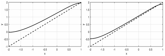
For illustration purpose, the asymptotics of the function for arbitrarily chosen values is provided in Figure 1.
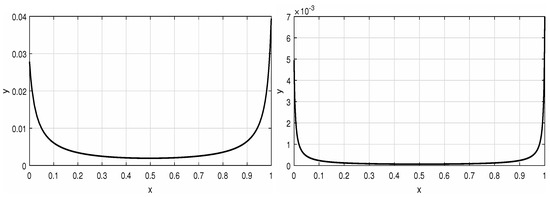
Figure 1.
Solution of BVP (9) with and (left) and (right). These functions reach their local minimum at a point asymptotically approaching .
In proving Theorems 3 and 4, we need the following statement about the uniform convergence of a sequence of convex functions and its derivative, which is a consequence of the theory of convex functions developed in [17,18]:
Lemma 3.
Let be convex functions on such that Then, converges uniformly to 0 on every closed interval
Proof.
It is known ([17], Lemma 1) that under the assumptions of the lemma, the sequence converges point-wise to 0 for The convexity of the functions () implies that each is non-decreasing and on I, where is the right end-point of the interval I and thus, the convergence of to 0 on I is uniform. □
2. Semilinear Singularly Perturbed Neumann Problem
We consider the semilinear Neumann BVP (3), namely
Theorem 2.
Assume that the reduced problem has an ()-stable solution of class . Then, there exists such that for every the BVP (3) has a solution , which, on the interval , satisfies
where is a solution of the nonhomogeneous Neumann BVP
and
Proof.
The theorem follows from Theorem 1 of the previous section, if we can exhibit, by construction, the existence of the lower and the upper bounding functions and with the required properties.
We now define, for x in and the functions
Here, where is a positive constant which is specified later.
It is easy to verify that the functions have the following properties: on the interval and they satisfy the boundary conditions required for upper and lower solutions for the BVP (3). Now, it remains to prove that and We treat the case where is ()-stable and consider .
From Taylor’s theorem and the hypothesis that is ()-stable, we have
where is a point between and for a sufficiently small say, for Since and are positive functions, we have
and so
for every If we choose a constant such that then
The verification for follows by symmetry. In detail, we have
where is a point between and and for sufficiently small say, for Then
The end of the proof is now the same as in the case of the lower bound The inequalities for and hold simultaneously if the parameter is from the interval where . The theorem is proved. □
Remark 3.
Lemma 2 implies that under the assumptions of Theorem 2, the solutions of semilinear Neumann BVP (3) converge uniformly on the interval to the solution of the reduced problem as
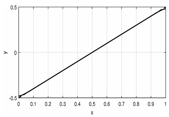
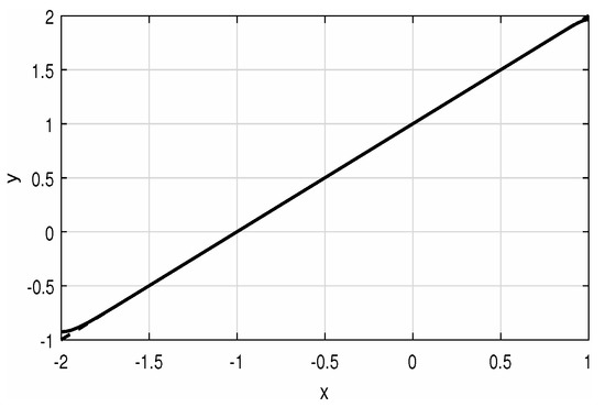
Example 1.
Let us consider the semilinear problem
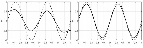
On the basis of Definition 2, the solution of the reduced problem, is ()-stable and Theorem 2 implies for every ε sufficiently small the existence of solutions which uniformly converge to the solution of the reduced problem. Figure 2 and Figure 3 document this convergence and also confirm the claim of Theorem 2 that as q increases, this convergence slows down.
Figure 2.
Solution of the semilinear Neumann problem (12) for and (left) and (right). The dashed line shows the function , the solution of the reduced problem.
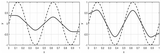
Figure 3.
Solution of the semilinear Neumann problem (12) for and (left) and (right). The dashed line shows the function , the solution of the reduced problem.
3. Quasi-linear Singularly Perturbed Neumann Problem
We consider now the singularly perturbed quasi-linear Neumann problem (4),
Theorem 3.
Assume that the reduced problem has an ()-stable solution of class . Let, for some ,
- for every if ; and
- for every if
Then, there exists such that for every , the BVP (4) has a solution , which, on the interval , satisfies
where is a solution of the nonhomogeneous Neumann BVP
and
where is a positive constant which is specified later.
Proof.
Define for x in and the functions
It is easy to check that and that , satisfy the boundary conditions required for upper and lower solutions for the BVP (4). From Taylor’s theorem and the ()-stability of the solution of the reduced problem , we have
and
Combining Lemma 2, Lemma 3 and the assumptions of the theorem, there exist positive constants and such that
on the interval and
on the interval for , so the inequalities
and
hold. The conclusion of the theorem now follows from Theorem 1. □
Example 2.
Let us consider the quasi-linear problem
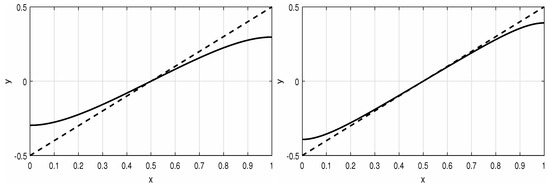
The general solution of the reduced problem is however, only satisfies the assumptions asked on the solution of the reduced problem. On the basis of Theorem 3, there exists such that for every , the problem has a solution satisfying on Figure 4 and Figure 5 show the convergence of the solutions to the solution of the reduced problem.
Figure 4.
Solution of the quasi-linear Neumann problem (13) with (left) and (right).
Figure 5.
Solution of the quasi-linear Neumann problem (13) with .
4. Quadratic Singularly Perturbed Neumann Problem
In this section, we investigate the asymptotic behavior of the solutions of the Neumann boundary value problem (5),
The novelty here is the presence of the quadratic term in . The more general differential equation
is not analyzed here, since it can be reduced to the form presented in (5) in some cases, by the usual device of completing the square. The decision to study the simpler equation rather than the more general equation stems from a desire to present a representative result for this “quadratic” class of problems without having to deal with extra complexities in notation.
Theorem 4.
Assume that the reduced problem has an ()-stable solution of class . Let, for some ,
- () for every if (); and
- () for every if ().
Then, there exists such that for every the BVP (5) has a solution , which, on the interval , satisfies
where is a solution of the nonhomogeneous Neumann BVP
and
where is a positive constant which is specified later.
Proof.
The idea of the proof is basically the same as in the proof of the previous theorem, so we focus only on its main points. For the functions
we obtain the inequalities
and
Similar to the proof of the previous theorem, we get that
on the interval and
on the interval for a sufficiently small and a suitable positive constant Therefore, for , we have
and
on the interval Theorem 4 is proved. □
Example 3.
For the quadratic problem
from the infinitely many solutions of the reduced problem , only satisfies the requirements from Theorem 4. This can also be deduced from the fact that the function is nondecreasing as a function of y for all and hence any two solutions of the Neumann problem (for a fixed ε) will differ only by a constant (Peano’s phenomenon [11]), and hence also in the limit for ε going to 0, the functions and will differ only by a constant, which is not possible from the form of the general solution of the reduced problem. Figure 6 and Figure 7 show the convergence of the solutions as implied by Theorem 4.
Figure 6.
Solution of the quadratic Neumann problem (14) with (left) and (right).
Figure 7.
Solution of the quadratic Neumann problem (14) with .
5. Conclusions
In this paper, we were concerned with establishing conditions guaranteeing the existence and uniform convergence of solutions of three types of Neumann boundary value problems, namely (3), (4) and (5). The analytical results in Theorem 2, Theorem 3 and Theorem 4, where, using the notion of the ()-stability of the solution of the reduced problem, the uniform convergence of the solutions to the solution of the reduced problem on the interval was proved.
Future research could focus on noninteger values of q in the definition of the ()-stability (Definition 2) but such that holds.
Funding
This publication has been published with the support of the Ministry of Education, Science, Research and Sport of the Slovak Republic within project VEGA 1/0193/22 “ Návrh identifikácie a systému monitorovania parametrov výrobných zariadení pre potreby prediktívnej údržby v súlade s konceptom Industry 4.0 s využitím technológií Industrial IoT ” and the Operational Program Integrated Infrastructure within project “ Výskum v sieti SANET a možnosti jej d’alšieho využitia a rozvoja ”, code ITMS 313011W988, cofinanced by the ERDF.
Institutional Review Board Statement
Not applicable.
Informed Consent Statement
Not applicable.
Data Availability Statement
Not applicable.
Acknowledgments
The author thanks the editors and five anonymous reviewers for their helpful feedback on earlier versions of this paper.
Conflicts of Interest
The author declares no conflict of interest.
References
- Ingram, S.K. Continuous dependence on parameters and boundary data for nonlinear two-point boundary value problems. Pac. J. Math. 1972, 41, 395–408. [Google Scholar] [CrossRef]
- Vasiliev, N.I.; Klokov, J.A. Foundations of the Theory of Boundary Value Problems for Ordinary Differential Equations; Zinatne: Riga, Latvia, 1978. (In Russian) [Google Scholar]
- Idczak, D. Stability in semilinear problems. J. Differ. Equ. 2000, 162, 64–90. [Google Scholar] [CrossRef]
- Chang, K.W.; Howes, F.A. Nonlinear Singular Perturbation Phenomena: Theory and Applications; Springer: New York, NY, USA, 1984. [Google Scholar]
- Nagumo, M. Über die Differentialgleichung y″ = f(x,y,y′). Proc. Phys. Math. Soc. Jpn. 1937, 19, 861–866. [Google Scholar]
- Fabry, C.; Mawhin, J.; Nkashama, M.N. A multiplicity result for periodic solutions of forced nonlinear second order ordinary differential equations. Bull. Lond. Math. Soc. 1986, 18, 173–180. [Google Scholar] [CrossRef]
- Hartman, P. Ordinary Differential Equations; Society for Industrial and Applied Mathematics (Classics in Applied Mathematics): Philadelphia, PA, USA, 2002. [Google Scholar]
- Bernstein, S.N. Sur les équations du calcul des variations. Ann. Sci. Ecole Norm. Sup. 1912, 29, 431–485. [Google Scholar] [CrossRef]
- Granas, A.; Guenther, R.B.; Lee, J.W. Nonlinear boundary value problems for some classes of ordinary differential equations. Rocky Mt. J. Math. 1980, 10, 35–58. [Google Scholar] [CrossRef]
- Granas, A.; Guenther, R.B.; Lee, J.W. On a theorem of S. Bernstein. Pac. J. Math. 1978, 74, 67–82. [Google Scholar] [CrossRef]
- Šeda, V. On some non-linear boundary value problems for ordinary differential equations. Arch. Math. 1989, 25, 207–222. [Google Scholar]
- Cabada, A. An Overview of the Lower and Upper Solutions Method with Nonlinear Boundary Value Conditions. Bound. Value Probl. 2011, 2011, 893753. [Google Scholar] [CrossRef]
- Cabada, A. A Positive Operator Approach to the Neumann Problem for a Second Order Ordinary Differential Equation. J. Math. Anal. Appl. 1996, 204, 774–785. [Google Scholar] [CrossRef]
- Dobkevich, M.; Sadyrbaev, F.; Sveikate, N.; Yermachenko, I. On Types of Solutions of the Second Order Nonlinear Boundary Value Problems. Abstr. Appl. Anal. 2014, 2014, 594931. [Google Scholar] [CrossRef]
- Bernfeld, S.R.; Chandra, J. Minimal and maximal solutions of nonlinear boundary value problems. Pac. J. Math. 1977, 71, 13–20. [Google Scholar] [CrossRef]
- Vrabel, R. Upper and lower solutions for singularly perturbed semilinear Neumann’s problem. Math. Bohem. 1997, 122, 175–180. [Google Scholar] [CrossRef]
- Tsuji, M. On F. Riesz’ fundamental theorem on subharmonic functions. Tohoku Math. J. 1952, 4, 131–140. [Google Scholar] [CrossRef]
- Rockafellar, R.T. Convex Analysis; Princeton University Press: Princeton, NJ, USA, 1970. [Google Scholar]
Disclaimer/Publisher’s Note: The statements, opinions and data contained in all publications are solely those of the individual author(s) and contributor(s) and not of MDPI and/or the editor(s). MDPI and/or the editor(s) disclaim responsibility for any injury to people or property resulting from any ideas, methods, instructions or products referred to in the content. |
© 2023 by the author. Licensee MDPI, Basel, Switzerland. This article is an open access article distributed under the terms and conditions of the Creative Commons Attribution (CC BY) license (https://creativecommons.org/licenses/by/4.0/).