Dynamic Behaviors of a COVID-19 and Influenza Co-Infection Model with Time Delays and Humoral Immunity

Abstract

Co-infections with respiratory viruses were reported in hospitalized patients in several cases. Severe acute respiratory syndrome coronavirus 2 (SARS-CoV-2) and influenza A virus (IAV) are two respiratory viruses and are similar in terms of their seasonal occurrence, clinical manifestations, transmission routes, and related immune responses. SARS-CoV-2 is the cause of coronavirus disease 2019 (COVID-19). In this paper, we study the dynamic behaviors of an influenza and COVID-19 co-infection model in vivo. The role of humoral (antibody) immunity in controlling the co-infection is modeled. The model considers the interactions among uninfected epithelial cells (ECs), SARS-CoV-2-infected ECs, IAV-infected ECs, SARS-CoV-2 particles, IAV particles, SARS-CoV-2 antibodies, and IAV antibodies. The model is given by a system of delayed ordinary differential equations (DODEs), which include four time delays: (i) a delay in the SARS-CoV-2 infection of ECs, (ii) a delay in the IAV infection of ECs, (iii) a maturation delay of newly released SARS-CoV-2 virions, and (iv) a maturation delay of newly released IAV virions. We establish the non-negativity and boundedness of the solutions. We examine the existence and stability of all equilibria. The Lyapunov method is used to prove the global stability of all equilibria. The theoretical results are supported by performing numerical simulations. We discuss the effects of antiviral drugs and time delays on the dynamics of influenza and COVID-19 co-infection. It is noted that increasing the delay length has a similar influence to that of antiviral therapies in eradicating co-infection from the body.

1. Introduction

Global health and economies have been severely affected since the emergence of the severe acute respiratory syndrome coronavirus 2 (SARS-CoV-2) in December 2019. This virus causes coronavirus disease 2019 (COVID-19), which swept the whole world with its rapid spread. Based on an update given by the World Health Organization (WHO) on 18 December 2022 [1], about 649 million confirmed cases and over 6.6 million deaths were reported globally. Influenza is another infectious respiratory disease that can cause serious morbidity and death. Influenza viruses of types A, B, C, and D infect about 20% of the world’s population in annual epidemics, resulting in 3–5 million severe illnesses and 290,000–650,000 deaths each year [2]. Influenza A virus (IAV) usually occurs in winter and is able to infect many species.

Epithelial cells (ECs) are the targets of both IAV and SARS-CoV-2 [3,4]. Both viruses have similar transmission paths. In addition, they have quite similar clinical manifestations, such as cough, myalgia, dyspnea, sore throat, headache, fever, and rhinitis [5]. Viral shedding often occurs within five to ten days in influenza, while it takes two to five weeks in COVID-19 [5]. Acute respiratory distress occurs more frequently in patients with COVID-19 than in those with influenza [5]. Less than 1% of influenza cases may die, while the death rate among COVID-19 patients is 3–4% [5]. The precautionary measures implemented by governments to limit the transmission of COVID-19 can play a role in reducing the transmission of influenza [6]. Currently, there are eleven vaccines for COVID-19 [7] and three types of influenza vaccines used worldwide [8].

One study by Zhu et al. [9] reported that 94.2% of COVID-19-infected individuals were also co-infected with many other types of microorganisms, such as viruses, fungi, and bacteria. Many co-infections of COVID-19 and influenza were reported in several studies [5,9,10,11,12] (see also the review articles [13,14,15,16]). Infection with multiple competitive respiratory viruses can cause the phenomenon of viral interference. It may happen that a certain type of virus has the ability to suppress the development and growth of another virus [17,18]. In [18,19], it was found that SARS-CoV-2 had a slower growth rate than that of IAV if the two infections started at the same time. If the influenza infection started after COVID-19, then influenza and COVID-19 co-infection could be detected. The progression and outcome of COVID-19 are highly dependent on a patient’s immunity. The risk of co-infection may be increased for persons who are immunocompromised [17]. In addition, Hashemi et al. [20] conducted a study that reported that, in patients with co-infection of influenza and COVID-19, the presence of underlying diseases, such as chronic neurological pathologies, diabetes, asthma, and heart disease, may lead to an increase in mortality.

Mathematical models of mono-infection or co-infection of viruses are important for understanding in-host viral infections and for developing antiviral drugs and vaccines. Models of in-host influenza mono-infection were formulated in many works (see the review papers [21,22,23,24]). Baccam et al. [25] presented a basic target-cell-limited influenza infection model. Several extensions were made for this model by incorporating the impacts of innate immunity [25,26], adaptive immunity [27,28], both innate and adaptive immunities [3,29,30,31,32], drug therapies [33], and time delays [34].

The model presented in [25] was used to describe the in-host COVID-19 dynamics in [35]. Li et al. [36] considered the regeneration and death of susceptible ECs. A model that was limited to target cells and a model with the regeneration and death of susceptible ECs were presented, respectively, in [35,36], where they were modified and extended by taking into account the influences of immune response [37,38,39,40,41,42,43,44], drug therapies [45,46,47], time delays [48], and reaction diffusion [49]. In [50], a two-state mathematical model of within-host SARS-CoV-2-neutralizing antibody dynamics in response to vaccination was considered. The stability of in-host COVID-19 mono-infection models was investigated in [41,42,43,48,51,52].

Pinky and Dobrovolny [18] constructed a SARS-CoV-2/IAV co-infection model that was limited to target cells. The authors mentioned that some types of respiratory viruses may be able to inhibit the progression of SARS-CoV-2. In [18], the effect of the immune response was not included. Moreover, the production and death of susceptible ECs were not considered. Elaiw et al. [53,54] examined the global properties of a SARS-CoV-2/IAV co-infection model with antibody immune response. However, a time delay was not considered in these papers. Time delay is one of the key factors for studying innovative insights into viral dynamics. In the process of SARS-CoV-2 and IAV infections, it takes time for the viruses to infect susceptible ECs and then release new mature viral particles. Therefore, it is important to include a time delay in COVID-19 and influenza co-infection models. The aim of this article is to construct a system of delayed differential equations (DDEs) that describe the in-host co-dynamics of influenza and COVID-19. The model extends the model presented in [53] by incorporating four time delays: (i) a delay in the SARS-CoV-2 infection of ECs, (ii) a delay in the IAV infection of ECs, (iii) a maturation delay of newly released SARS-CoV-2 virions, and (iv) a maturation delay of newly released IAV virions. We first investigate the basic properties of the DDEs; then, we find all equilibria and examine their global stability. We illustrate the theoretical results via numerical simulations. The effects of time delays on the dynamics of COVID-19 and influenza co-infection are discussed.

2. Model Formulation

This section develops a system of DDEs that describe influenza and COVID-19 co-infection with four time delays. Let t represent the time and let $X\left(t\right)$, $Y\left(t\right)$, $I\left(t\right)$, $V\left(t\right)$, $P\left(t\right)$, $Z\left(t\right)$, and $M\left(t\right)$ represent the concentrations of susceptible ECs, SARS-CoV-2-infected ECs, IAV-infected ECs, SARS-CoV-2 particles, IAV particles, SARS-CoV-2 antibodies, and IAV antibodies. The following system of DDEs is to be studied:

$$\begin{array}{cc}\hfill \frac{dX\left(t\right)}{dt}& =\stackrel{\mathrm{ECs}\mathrm{production}}{\overbrace{\delta }}-\stackrel{\mathrm{natural}\mathrm{death}}{\overbrace{\varrho X\left(t\right)}}-\stackrel{\mathrm{SARS}-\mathrm{CoV}-2\mathrm{infectious}\mathrm{transmission}}{\overbrace{{\xi }_{V}X\left(t\right)V\left(t\right)}}-\stackrel{\mathrm{IAV}\mathrm{infectious}\mathrm{transmission}}{\overbrace{{\xi }_{P}X\left(t\right)P\left(t\right)}},\hfill \end{array}$$

(1)

$$\begin{array}{cc}\hfill \frac{dY\left(t\right)}{dt}& =\stackrel{\mathrm{SARS}-\mathrm{CoV}-2\mathrm{infectious}\mathrm{transmission}}{\overbrace{e^{-{\alpha }_1{\tau }_1}{\xi }_{V}X(t-{\tau }_1)V(t-{\tau }_1)}}-\stackrel{\mathrm{natural}\mathrm{death}}{\overbrace{{\beta }_{Y}Y\left(t\right)}},\hfill \end{array}$$

(2)

$$\begin{array}{cc}\hfill \frac{dI\left(t\right)}{dt}& =\stackrel{\mathrm{IAV}\mathrm{infectious}\mathrm{transmission}}{\overbrace{e^{-{\alpha }_3{\tau }_3}{\xi }_{P}X(t-{\tau }_3)P(t-{\tau }_3)}}-\stackrel{\mathrm{natural}\mathrm{death}}{\overbrace{{\beta }_{I}I\left(t\right)}},\hfill \end{array}$$

(3)

$$\begin{array}{cc}\hfill \frac{dV\left(t\right)}{dt}& =\stackrel{\mathrm{SARS}-\mathrm{CoV}-2\mathrm{production}}{\overbrace{e^{-{\alpha }_2{\tau }_2}{\theta }_{V}Y(t-{\tau }_2)}}-\stackrel{\mathrm{natural}\mathrm{death}}{\overbrace{{\lambda }_{V}V\left(t\right)}}-\stackrel{\mathrm{SARS}-\mathrm{CoV}-2\mathrm{neutralization}}{\overbrace{{\rho }_{V}V\left(t\right)Z\left(t\right)}},\hfill \end{array}$$

(4)

$$\begin{array}{cc}\hfill \frac{dP\left(t\right)}{dt}& =\stackrel{\mathrm{IAV}\mathrm{production}}{\overbrace{e^{-{\alpha }_4{\tau }_4}{\theta }_{P}I(t-{\tau }_4)}}-\stackrel{\mathrm{natural}\mathrm{death}}{\overbrace{{\lambda }_{P}P\left(t\right)}}-\stackrel{\mathrm{IAV}\mathrm{neutralization}}{\overbrace{{\rho }_{P}P\left(t\right)M\left(t\right)}},\hfill \end{array}$$

(5)

$$\begin{array}{cc}\hfill \frac{dZ\left(t\right)}{dt}& =\stackrel{\mathrm{proliferation}\mathrm{SARS}-\mathrm{CoV}-2\mathrm{antibodies}}{\overbrace{{\eta }_{Z}V\left(t\right)Z\left(t\right)}}-\stackrel{\mathrm{natural}\mathrm{death}}{\overbrace{{\gamma }_{Z}Z\left(t\right)}},\hfill \end{array}$$

(6)

$$\begin{array}{cc}\hfill \frac{dM\left(t\right)}{dt}& =\stackrel{\mathrm{proliferation}\mathrm{IAV}\mathrm{antibodies}}{\overbrace{{\eta }_{M}P\left(t\right)M\left(t\right)}}-\stackrel{\mathrm{natural}\mathrm{death}}{\overbrace{{\gamma }_{M}M\left(t\right)}}.\hfill \end{array}$$

(7)

Here, ${\tau }_1$ and ${\tau }_3$ are the delays between the entries of SARS-CoV-2 and IAV into ECs and the start of production of immature SARS-CoV-2 and IAV virions, respectively. ${\tau }_2$ and ${\tau }_4$ are the maturation delays of newly released SARS-CoV-2 and IAV virions, respectively. The probabilities of SARS-CoV-2-infected ECs and IAV-infected ECs surviving to the ages of ${\tau }_1$ and ${\tau }_3$ are represented by $e^{-{\alpha }_1{\tau }_1}$ and $e^{-{\alpha }_3{\tau }_3}$, respectively. The probabilities of released SARS-CoV-2 and IAV virions surviving to the ages ${\tau }_2$ and ${\tau }_4$ are denoted by $e^{-{\alpha }_2{\tau }_2}$ and $e^{-{\alpha }_4{\tau }_4}$, respectively.

The initial states (conditions) for system (1)–(7) are given as:

$$\begin{array}{cc}\hfill X\left(u\right)& ={\psi }_1\left(u\right),Y\left(u\right)={\psi }_2\left(u\right),I\left(u\right)={\psi }_3\left(u\right),V\left(u\right)={\psi }_4\left(u\right),\hfill \\ \hfill P\left(u\right)& ={\psi }_5\left(u\right),Z\left(u\right)={\psi }_6\left(u\right),M\left(u\right)={\psi }_7\left(u\right),\hfill \\ \hfill {\psi }_i\left(u\right)& \ge 0,u\in \left[-{\tau }^{*},0\right],\hfill \\ \hfill {\psi }_i\left(u\right)& \in C\left(\left[-{\tau }^{*},0\right],{\mathbb{R}}_{\ge 0}\right),i=1,2,\cdots ,7,\hfill \end{array}$$

(8)

where ${\tau }^{*}=max\{{\tau }_1,{\tau }_2,{\tau }_3,{\tau }_4\}$, and C is the Banach space of continuous functions mapping the interval $\left[-{\tau }^{*},0\right]$ into ${\mathbb{R}}_{\ge 0}$ with $∥{\psi }_i∥={sup}_{-{\tau }^{*}\le u\le 0}\left|{\psi }_i\left(u\right)\right|$ for ${\psi }_i\in C$. We note that system (1)–(7), with initial conditions (8), has a unique solution [55].

3. Well-Posedness of the Solutions

Here, we investigate the non-negativity and ultimate boundedness of system (1)–(7).

Lemma 1.

The solutions of system (1)–(7) with initial states (8) are non-negative and ultimately bounded.

Proof. 

We have that

$$\frac{dX}{dt}{\mid }_{X=0}=\delta >0,\frac{dZ}{dt}{\mid }_{Z=0}=0,\frac{dM}{dt}{\mid }_{M=0}=0.$$

Hence, $X\left(t\right),Z\left(t\right),M\left(t\right)\ge 0$ for all $t\ge 0$. Moreover, for all $t\in \left[0,{\tau }^{*}\right],$ we have:

$$\begin{array}{cc}\hfill Y\left(t\right)& ={\psi }_2\left(0\right)e^{-{\beta }_{Y}t}+{\xi }_V{e}^{-{\alpha }_1{\tau }_1}{\displaystyle \underset{0}{\overset{t}{\int }}}{e}^{-{\beta }_Y(t-u)}X\left(u-{\tau }_1\right)V\left(u-{\tau }_1\right)du\ge 0,\hfill \\ \hfill I\left(t\right)& ={\psi }_3\left(0\right)e^{-{\beta }_{I}t}+{\xi }_P{e}^{-{\alpha }_3{\tau }_3}{\displaystyle \underset{0}{\overset{t}{\int }}}{e}^{-{\beta }_I(t-u)}X\left(u-{\tau }_3\right)P\left(u-{\tau }_3\right)du\ge 0,\hfill \\ \hfill V\left(t\right)& ={\psi }_4\left(0\right)e^{-{\int }_0^t\left({\lambda }_V+{\rho }_{V}Z\left(r\right)\right)dr}+{\theta }_V{e}^{-{\alpha }_2{\tau }_2}{\displaystyle \underset{0}{\overset{t}{\int }}}{e}^{-{\int }_u^t\left({\lambda }_V+{\rho }_{V}Z\left(r\right)\right)dr}Y\left(u-{\tau }_2\right)du\ge 0,\hfill \\ \hfill P\left(t\right)& ={\psi }_5\left(0\right)e^{-{\int }_0^t\left({\lambda }_P+{\rho }_{P}M\left(r\right)\right)dr}+{\theta }_P{e}^{-{\alpha }_4{\tau }_4}{\displaystyle \underset{0}{\overset{t}{\int }}}{e}^{-{\int }_u^t\left({\lambda }_P+{\rho }_{P}M\left(r\right)\right)dr}I\left(u-{\tau }_4\right)du\ge 0.\hfill \end{array}$$

Hence, $Y\left(t\right),I\left(t\right),V\left(t\right),P\left(t\right)\ge 0$ for all $t\in \left[0,{\tau }^{*}\right]$. Through recursive argumentation, we get $Y\left(t\right),I\left(t\right),V\left(t\right),P\left(t\right)$ for all $t\ge 0.$ Therefore, $X,Y,I,V,P,Z$, and M are non-negative.

The non-negativity of the system’s solution implies that:

$$\frac{dX\left(t\right)}{dt}\le \delta -\varrho X⟹\underset{t\to \infty }{lim}supX\left(t\right)=\frac{\delta }{\varrho }.$$

Let us define

$${\mathsf{\Psi }}_1\left(t\right)=e^{-{\alpha }_1{\tau }_1}X\left(t-{\tau }_1\right)+Y\left(t\right).$$

Then,

$$\begin{array}{cc}\hfill \frac{d{\mathsf{\Psi }}_1\left(t\right)}{dt}& =e^{-{\alpha }_1{\tau }_1}\delta -e^{-{\alpha }_1{\tau }_1}\varrho X\left(t-{\tau }_1\right)-e^{-{\alpha }_1{\tau }_1}{\xi }_{P}X\left(t-{\tau }_1\right)P\left(t-{\tau }_1\right)-{\beta }_{Y}Y\left(t\right)\hfill \\ \hfill & \le \delta -e^{-{\alpha }_1{\tau }_1}\varrho X\left(t-{\tau }_1\right)-{\beta }_{Y}Y\left(t\right)\hfill \\ \hfill & \le \delta -{\phi }_1\left[e^{-{\alpha }_1{\tau }_1}X\left(t-{\tau }_1\right)+Y\left(t\right)\right]=\delta -{\phi }_1{\mathsf{\Psi }}_1\left(t\right),\hfill \end{array}$$

where ${\phi }_1=min\{\varrho ,{\beta }_Y\}$. This implies that

$$\underset{t\to \infty }{lim}sup{\mathsf{\Psi }}_1\left(t\right)\le \frac{\delta }{{\phi }_1}=A_1⟹\underset{t\to \infty }{lim}supY\left(t\right)\le A_1.$$

Let

$$\begin{array}{cc}\hfill {\mathsf{\Psi }}_2\left(t\right)& =e^{-{\alpha }_3{\tau }_3}X\left(t-{\tau }_3\right)+I\left(t\right)\hfill \\ \hfill \frac{d{\mathsf{\Psi }}_2\left(t\right)}{dt}& =e^{-{\alpha }_3{\tau }_3}\delta -e^{-{\alpha }_3{\tau }_3}\varrho X\left(t-{\tau }_3\right)-e^{-{\alpha }_3{\tau }_3}{\xi }_{V}X\left(t-{\tau }_3\right)V\left(t-{\tau }_3\right)-{\beta }_{I}I\left(t\right)\hfill \\ \hfill & \le \delta -e^{-{\alpha }_3{\tau }_3}\varrho X\left(t-{\tau }_3\right)-{\beta }_{I}I\left(t\right)\hfill \\ \hfill & \le \delta -{\phi }_2\left[e^{-{\alpha }_3{\tau }_3}X\left(t-{\tau }_3\right)+I\left(t\right)\right]=\delta -{\phi }_2{\mathsf{\Psi }}_2\left(t\right),\hfill \end{array}$$

where ${\phi }_2=min\{\varrho ,{\beta }_I\}$. It follows that

$$\underset{t\to \infty }{lim}sup{\mathsf{\Psi }}_2\left(t\right)\le \frac{\delta }{{\phi }_2}=A_2⟹\underset{t\to \infty }{lim}supI\left(t\right)\le A_2.$$

Let us define

$$\begin{array}{cc}\hfill {\mathsf{\Psi }}_3\left(t\right)& =V\left(t\right)+P\left(t\right)+\frac{{\rho }_V}{{\eta }_Z}Z\left(t\right)+\frac{{\rho }_P}{{\eta }_M}M\left(t\right).\hfill \\ \hfill \frac{d{\mathsf{\Psi }}_3\left(t\right)}{dt}& =e^{-{\alpha }_2{\tau }_2}{\theta }_{V}Y\left(t-{\tau }_2\right)-{\lambda }_{V}V\left(t\right)+e^{-{\alpha }_4{\tau }_4}{\theta }_{P}I\left(t-{\tau }_4\right)-{\lambda }_{P}P\left(t\right)-\frac{{\rho }_V{\gamma }_Z}{{\eta }_Z}Z\left(t\right)\hfill \\ \hfill & -\frac{{\rho }_P{\gamma }_M}{{\eta }_M}M\left(t\right).\hfill \end{array}$$

Since $Y\left(t\right)\le A_1,I\left(t\right)\le A_2,$ then

$$\begin{array}{cc}\hfill \frac{d{\mathsf{\Psi }}_3\left(t\right)}{dt}& \le {\theta }_V{A}_1+{\theta }_P{A}_2-{\lambda }_{V}V\left(t\right)-{\lambda }_{P}P\left(t\right)-\frac{{\rho }_V{\gamma }_Z}{{\eta }_Z}Z\left(t\right)-\frac{{\rho }_P{\gamma }_M}{{\eta }_M}M\left(t\right)\hfill \\ \hfill & \le {\theta }_V{A}_1+{\theta }_P{A}_2-{\phi }_3\left[V\left(t\right)+P\left(t\right)+\frac{{\rho }_V}{{\eta }_Z}Z\left(t\right)+\frac{{\rho }_P}{{\eta }_M}M\left(t\right)\right]\hfill \\ \hfill & ={\theta }_V{A}_1+{\theta }_P{A}_2-{\phi }_3{\mathsf{\Psi }}_3\left(t\right)\hfill \end{array}$$

where ${\phi }_3=min\{{\lambda }_V,{\lambda }_P,{\gamma }_Z,{\gamma }_M\}$. Then, we get

$$\underset{t\to \infty }{lim}sup{\mathsf{\Psi }}_3\left(t\right)\le \frac{{\theta }_V{A}_1+{\theta }_P{A}_2}{{\phi }_3}=A_3.$$

Since $V\left(t\right)>0,P\left(t\right)>0,Z\left(t\right)>0$ and $M\left(t\right)>0$, then

$$\begin{array}{cc}\hfill \underset{t\to \infty }{lim}supV\left(t\right)& \le A_3,\underset{t\to \infty }{lim}supP\left(t\right)\le A_3,\hfill \\ \hfill \underset{t\to \infty }{lim}supZ\left(t\right)& \le \frac{{\eta }_Z}{{\rho }_V}{A}_3=A_4\mathrm{and}\underset{t\to \infty }{lim}supM\left(t\right)\le \frac{{\eta }_M}{{\rho }_P}{A}_3=A_5.\hfill \end{array}$$

□

Based on Lemma 1, we can show that the domain

$$\begin{array}{cc}\hfill \mathsf{\Phi }& =\{\left(X,Y,I,V,P,Z,M\right)\in C_{\ge 0}^7:∥X∥,∥Y∥\le A_1,∥I∥\le A_2,∥V∥,∥P∥\le A_3,∥Z∥\le A_4,\hfill \\ \hfill & ∥M∥\le A_5\}\hfill \end{array}$$

is positively invariant for model (1)–(7).

4. Equilibria

Here, we calculate the system’s equilibria and deduce the condition of their existence. Any equilibrium point $\mathsf{\Delta }=(X,Y,I,V,P,Z,M)$ satisfies:

$$\begin{array}{cc}\hfill 0& =\delta -\varrho X-{\xi }_{V}XV-{\xi }_{P}XP,\hfill \end{array}$$

(9)

$$\begin{array}{cc}\hfill 0& =e^{-{\alpha }_1{\tau }_1}{\xi }_{V}XV-{\beta }_{Y}Y,\hfill \end{array}$$

(10)

$$\begin{array}{cc}\hfill 0& =e^{-{\alpha }_3{\tau }_3}{\xi }_{P}XP-{\beta }_{I}I,\hfill \end{array}$$

(11)

$$\begin{array}{cc}\hfill 0& =e^{-{\alpha }_2{\tau }_2}{\theta }_{V}Y-{\lambda }_{V}V-{\rho }_{V}VZ,\hfill \end{array}$$

(12)

$$\begin{array}{cc}\hfill 0& =e^{-{\alpha }_4{\tau }_4}{\theta }_{P}I-{\lambda }_{P}P-{\rho }_{P}PM,\hfill \end{array}$$

(13)

$$\begin{array}{cc}\hfill 0& ={\eta }_{Z}VZ-{\gamma }_{Z}Z,\hfill \end{array}$$

(14)

$$\begin{array}{cc}\hfill 0& ={\eta }_{M}PM-{\gamma }_{M}M.\hfill \end{array}$$

(15)

Solving Equations (9)–(15), we get eight equilibria.

(i) Infection-free equilibrium, ${\mathsf{\Delta }}_0=(X_0,0,0,0,0,0,0)$, where $X_0=\delta /\varrho$.

(ii) COVID-19 mono-infection equilibrium with inactive antibody response ${\mathsf{\Delta }}_1=(X_1,Y_1,0,V_1,0,0,0),$ where

$$\begin{array}{cc}\hfill X_1& =\frac{{\beta }_Y{\lambda }_V}{e^{-{\alpha }_1{\tau }_1-{\alpha }_2{\tau }_2}{\theta }_V{\xi }_V},Y_1=\frac{\varrho {\lambda }_V}{e^{-{\alpha }_2{\tau }_2}{\theta }_V{\xi }_V}\left[\frac{e^{-{\alpha }_1{\tau }_1-{\alpha }_2{\tau }_2}{X}_0{\theta }_V{\xi }_V}{{\beta }_Y{\lambda }_V}-1\right],\hfill \\ \hfill V_1& =\frac{\varrho }{{\xi }_V}\left[\frac{e^{-{\alpha }_1{\tau }_1-{\alpha }_2{\tau }_2}{X}_0{\theta }_V{\xi }_V}{{\beta }_Y{\lambda }_V}-1\right].\hfill \end{array}$$

Therefore, $Y_1>0$ and $V_1>0$ when

$$\frac{e^{-{\alpha }_1{\tau }_1-{\alpha }_2{\tau }_2}{X}_0{\theta }_V{\xi }_V}{{\beta }_Y{\lambda }_V}>1.$$

We define the basic COVID-19 mono-infection reproduction number as:

$${\Re }_1=\frac{e^{-{\alpha }_1{\tau }_1-{\alpha }_2{\tau }_2}{X}_0{\theta }_V{\xi }_V}{{\beta }_Y{\lambda }_V}.$$

Thus, we can write:

$$X_1=\frac{X_0}{{\Re }_1},Y_1=\frac{\varrho {\lambda }_V}{e^{-{\alpha }_2{\tau }_2}{\theta }_V{\xi }_V}\left({\Re }_1-1\right),V_1=\frac{\varrho }{{\xi }_V}\left({\Re }_1-1\right).$$

Consequently, ${\mathsf{\Delta }}_1$ exists if ${\Re }_1>1.$

(iii) Influenza mono-infection equilibrium with inactive antibody response, ${\mathsf{\Delta }}_2=(X_2,0,I_2,0,P_2,0,0)$, where

$$\begin{array}{cc}\hfill X_2& =\frac{{\beta }_I{\lambda }_P}{e^{-{\alpha }_3{\tau }_3-{\alpha }_4{\tau }_4}{\theta }_P{\xi }_P},I_2=\frac{\varrho {\lambda }_P}{e^{-{\alpha }_4{\tau }_4}{\theta }_P{\xi }_P}\left[\frac{e^{-{\alpha }_3{\tau }_3-{\alpha }_4{\tau }_4}{X}_0{\theta }_P{\xi }_P}{{\beta }_I{\lambda }_P}-1\right],\hfill \\ \hfill P_2& =\frac{\varrho }{{\xi }_P}\left[\frac{e^{-{\alpha }_3{\tau }_3-{\alpha }_4{\tau }_4}{X}_0{\theta }_P{\xi }_P}{{\beta }_I{\lambda }_P}-1\right].\hfill \end{array}$$

Therefore, $I_2>0$ and $P_2>0$ when

$$\frac{e^{-{\alpha }_3{\tau }_3-{\alpha }_4{\tau }_4}{X}_0{\theta }_P{\xi }_P}{{\beta }_I{\lambda }_P}>1.$$

We define the basic influenza mono-infection reproduction number as:

$${\Re }_2=\frac{e^{-{\alpha }_3{\tau }_3-{\alpha }_4{\tau }_4}{X}_0{\theta }_P{\xi }_P}{{\beta }_I{\lambda }_P}.$$

In terms of ${\Re }_2$, we write

$$X_2=\frac{X_0}{{\Re }_2},I_2=\frac{\varrho {\lambda }_P}{e^{-{\alpha }_4{\tau }_4}{\theta }_P{\xi }_P}\left({\Re }_2-1\right),P_2=\frac{\varrho }{{\xi }_P}\left({\Re }_2-1\right).$$

Therefore, ${\mathsf{\Delta }}_2$ exists if ${\Re }_2>1.$

(iv) COVID-19 mono-infection equilibrium with activated SARS-CoV-2-specific antibody response, ${\mathsf{\Delta }}_3=(X_3,Y_3,0,V_3,0,Z_3,0)$, where

$$\begin{array}{cc}\hfill X_3& =\frac{\delta {\eta }_Z}{{\xi }_V{\gamma }_Z+\varrho {\eta }_Z},Y_3=\frac{e^{-{\alpha }_1{\tau }_1}\delta {\xi }_V{\gamma }_Z}{{\beta }_Y\left({\xi }_V{\gamma }_Z+\varrho {\eta }_Z\right)},\hfill \\ \hfill V_3& =\frac{{\gamma }_Z}{{\eta }_Z},Z_3=\frac{{\lambda }_V}{{\rho }_V}\left[\frac{e^{-{\alpha }_1{\tau }_1-{\alpha }_2{\tau }_2}\delta {\xi }_V{\eta }_Z{\theta }_V}{{\beta }_Y{\lambda }_V\left({\xi }_V{\gamma }_Z+\varrho {\eta }_Z\right)}-1\right].\hfill \end{array}$$

We note that ${\mathsf{\Delta }}_3$ exists when

$$\frac{e^{-{\alpha }_1{\tau }_1-{\alpha }_2{\tau }_2}\delta {\xi }_V{\eta }_Z{\theta }_V}{{\beta }_Y{\lambda }_V\left({\xi }_V{\gamma }_Z+\varrho {\eta }_Z\right)}>1.$$

Let us define the SARS-CoV-2-specific antibody response activation number for COVID-19 mono-infection as:

$${\Re }_3=\frac{e^{-{\alpha }_1{\tau }_1-{\alpha }_2{\tau }_2}\delta {\xi }_V{\eta }_Z{\theta }_V}{{\beta }_Y{\lambda }_V\left({\xi }_V{\gamma }_Z+\varrho {\eta }_Z\right)}.$$

Thus, $Z_3=\frac{{\lambda }_V}{{\rho }_V}\left({\Re }_3-1\right)$.

(v) Influenza mono-infection equilibrium with activation of of IAV-specific antibody response, ${\mathsf{\Delta }}_4=(X_4,0,I_4,0,P_4,0,M_4)$, where

$$\begin{array}{cc}\hfill X_4& =\frac{\delta {\eta }_M}{{\xi }_P{\gamma }_M+\varrho {\eta }_M},I_4=\frac{e^{-{\alpha }_3{\tau }_3}\delta {\xi }_P{\gamma }_M}{{\beta }_I\left({\xi }_P{\gamma }_M+\varrho {\eta }_M\right)},\hfill \\ \hfill P_4& =\frac{{\gamma }_M}{{\eta }_M},M_4=\frac{{\lambda }_P}{{\rho }_P}\left[\frac{e^{-{\alpha }_3{\tau }_3-{\alpha }_4{\tau }_4}\delta {\xi }_P{\eta }_M{\theta }_P}{{\beta }_I{\lambda }_P\left({\xi }_P{\gamma }_M+\varrho {\eta }_M\right)}-1\right].\hfill \end{array}$$

We note that ${\mathsf{\Delta }}_4$ exists when

$$\frac{e^{-{\alpha }_3{\tau }_3-{\alpha }_4{\tau }_4}\delta {\xi }_P{\eta }_M{\theta }_P}{{\beta }_I{\lambda }_P\left({\xi }_P{\gamma }_M+\varrho {\eta }_M\right)}>1.$$

The IAV-specific antibody response activation number for influenza mono-infection is defined as:

$${\Re }_4=\frac{e^{-{\alpha }_3{\tau }_3-{\alpha }_4{\tau }_4}\delta {\xi }_P{\eta }_M{\theta }_P}{{\beta }_I{\lambda }_P\left({\xi }_P{\gamma }_M+\varrho {\eta }_M\right)}.$$

Thus, $M_4=\frac{{\lambda }_P}{{\rho }_P}\left({\Re }_4-1\right)$.

(vi) Influenza and COVID-19 co-infection equilibrium with only the activated SARS-CoV-2-specific antibody response, ${\mathsf{\Delta }}_5=(X_5,Y_5,I_5,V_5,P_5,Z_5,0)$, where

$$\begin{array}{cc}\hfill X_5& =\frac{{\beta }_I{\lambda }_P}{e^{-{\alpha }_3{\tau }_3-{\alpha }_4{\tau }_4}{\theta }_P{\xi }_P},Y_5=\frac{e^{-{\alpha }_1{\tau }_1}{\xi }_V{\beta }_I{\lambda }_P{\gamma }_Z}{e^{-{\alpha }_3{\tau }_3-{\alpha }_4{\tau }_4}{\theta }_P{\xi }_P{\beta }_Y{\eta }_Z},\hfill \\ \hfill I_5& =\frac{{\lambda }_P({\xi }_V{\gamma }_Z+\varrho {\eta }_Z)}{e^{-{\alpha }_4{\tau }_4}{\theta }_P{\xi }_P{\eta }_Z}\left[\frac{e^{-{\alpha }_3{\tau }_3-{\alpha }_4{\tau }_4}\delta {\xi }_P{\theta }_P{\eta }_Z}{{\beta }_I{\lambda }_P({\xi }_V{\gamma }_Z+\varrho {\eta }_Z)}-1\right],V_5=\frac{{\gamma }_Z}{{\eta }_Z},\hfill \\ \hfill P_5& =\frac{{\xi }_V{\gamma }_Z+\varrho {\eta }_Z}{{\xi }_P{\eta }_Z}\left[\frac{e^{-{\alpha }_3{\tau }_3-{\alpha }_4{\tau }_4}\delta {\xi }_P{\theta }_P{\eta }_Z}{{\beta }_I{\lambda }_P\left({\xi }_V{\gamma }_Z+\varrho {\eta }_Z\right)}-1\right],\hfill \\ \hfill Z_5& =\frac{{\lambda }_V}{{\rho }_V}\left[\frac{e^{-{\alpha }_1{\tau }_1-{\alpha }_2{\tau }_2}{\theta }_V{\xi }_V{\beta }_I{\lambda }_P}{e^{-{\alpha }_3{\tau }_3-{\alpha }_4{\tau }_4}{\theta }_P{\xi }_P{\beta }_Y{\lambda }_V}-1\right]=\frac{{\lambda }_V}{{\rho }_V}\left({\Re }_1/{\Re }_2-1\right).\hfill \end{array}$$

Hence, ${\mathsf{\Delta }}_5$ exists when

$$\frac{{\Re }_1}{{\Re }_2}>1\mathrm{and}\frac{e^{-{\alpha }_3{\tau }_3-{\alpha }_4{\tau }_4}\delta {\xi }_P{\theta }_P{\eta }_Z}{{\beta }_I{\lambda }_P\left({\xi }_V{\gamma }_Z+\varrho {\eta }_Z\right)}>1.$$

The influenza infection reproduction number in the presence of COVID-19 infection is stated as:

$${\Re }_5=\frac{e^{-{\alpha }_3{\tau }_3-{\alpha }_4{\tau }_4}\delta {\xi }_P{\theta }_P{\eta }_Z}{{\beta }_I{\lambda }_P\left({\xi }_V{\gamma }_Z+\varrho {\eta }_Z\right)}.$$

Hence,

$$I_5=\frac{{\lambda }_P({\xi }_V{\gamma }_Z+\varrho {\eta }_Z)}{e^{-{\alpha }_4{\tau }_4}{\theta }_P{\xi }_P{\eta }_Z}\left({\Re }_5-1\right),P_5=\frac{{\xi }_V{\gamma }_Z+\varrho {\eta }_Z}{{\xi }_P{\eta }_Z}\left({\Re }_5-1\right),$$

and then ${\mathsf{\Delta }}_5$ exists if $\frac{{\Re }_1}{{\Re }_2}>1$ and ${\Re }_5>1$.

(vii) Influenza and COVID-19 co-infection equilibrium with only the activated IAV-specific antibody response, ${\mathsf{\Delta }}_6=(X_6,Y_6,I_6,V_6,P_6,0,M_6)$, where

$$\begin{array}{cc}\hfill X_6& =\frac{{\beta }_Y{\lambda }_V}{e^{-{\alpha }_1{\tau }_1-{\alpha }_2{\tau }_2}{\theta }_V{\xi }_V},Y_6=\frac{{\lambda }_V\left({\xi }_P{\gamma }_M+\varrho {\eta }_M\right)}{e^{-{\alpha }_2{\tau }_2}{\theta }_V{\xi }_V{\eta }_M}\left[\frac{e^{-{\alpha }_1{\tau }_1-{\alpha }_2{\tau }_2}\delta {\xi }_V{\theta }_V{\eta }_M}{{\beta }_Y{\lambda }_V({\xi }_P{\gamma }_M+\varrho {\eta }_M)}-1\right],\hfill \\ \hfill I_6& =\frac{e^{-{\alpha }_3{\tau }_3}{\xi }_P{\gamma }_M{\beta }_Y{\lambda }_V}{e^{-{\alpha }_1{\tau }_1-{\alpha }_2{\tau }_2}{\theta }_V{\xi }_V{\beta }_I{\eta }_M},V_6=\frac{{\xi }_P{\gamma }_M+\varrho {\eta }_M}{{\xi }_V{\eta }_M}\left[\frac{e^{-{\alpha }_1{\tau }_1-{\alpha }_2{\tau }_2}\delta {\xi }_V{\theta }_V{\eta }_M}{{\beta }_Y{\lambda }_V({\xi }_P{\gamma }_M+\varrho {\eta }_M)}-1\right],\hfill \\ \hfill P_6& =\frac{{\gamma }_M}{{\eta }_M},M_6=\frac{{\lambda }_P}{{\rho }_P}\left[\frac{e^{-{\alpha }_3{\tau }_3-{\alpha }_4{\tau }_4}{\theta }_P{\xi }_P{\beta }_Y{\lambda }_V}{e^{-{\alpha }_1{\tau }_1-{\alpha }_2{\tau }_2}{\theta }_V{\xi }_V{\beta }_I{\lambda }_P}-1\right]=\frac{{\lambda }_P}{{\rho }_P}\left({\Re }_2/{\Re }_1-1\right).\hfill \end{array}$$

We note that ${\mathsf{\Delta }}_6$ exists when

$$\frac{{\Re }_2}{{\Re }_1}>1\mathrm{and}\frac{e^{-{\alpha }_1{\tau }_1-{\alpha }_2{\tau }_2}\delta {\xi }_V{\theta }_V{\eta }_M}{{\beta }_Y{\lambda }_V({\xi }_P{\gamma }_M+\varrho {\eta }_M)}>1.$$

The COVID-19 infection reproduction number in the presence of influenza infection is stated as:

$${\Re }_6=\frac{e^{-{\alpha }_1{\tau }_1-{\alpha }_2{\tau }_2}\delta {\xi }_V{\theta }_V{\eta }_M}{{\beta }_Y{\lambda }_V({\xi }_P{\gamma }_M+\varrho {\eta }_M)}.$$

Thus,

$$Y_6=\frac{{\lambda }_V\left({\xi }_P{\gamma }_M+\varrho {\eta }_M\right)}{e^{-{\alpha }_2{\tau }_2}{\theta }_V{\xi }_V{\eta }_M}\left({\Re }_6-1\right),V_6=\frac{{\xi }_P{\gamma }_M+\varrho {\eta }_M}{{\xi }_V{\eta }_M}\left({\Re }_6-1\right).$$

(viii) Influenza and COVID-19 co-infection equilibrium with activation of both SARS-CoV-2 and IAV antibody responses ${\mathsf{\Delta }}_7=(X_7,Y_7,I_7,V_7,P_7,Z_7,M_7)$, where

$$\begin{array}{cc}\hfill X_7& =\frac{\delta {\eta }_Z{\eta }_M}{{\xi }_P{\gamma }_M{\eta }_Z+{\xi }_V{\gamma }_Z{\eta }_M+\varrho {\eta }_Z{\eta }_M},Y_7=\frac{e^{-{\alpha }_1{\tau }_1}\delta {\xi }_V{\gamma }_Z{\eta }_M}{{\beta }_Y\left({\xi }_P{\gamma }_M{\eta }_Z+{\xi }_V{\gamma }_Z{\eta }_M+\varrho {\eta }_Z{\eta }_M\right)},\hfill \\ \hfill I_7& =\frac{e^{-{\alpha }_3{\tau }_3}\delta {\xi }_P{\gamma }_M{\eta }_Z}{{\beta }_I\left({\xi }_P{\gamma }_M{\eta }_Z+{\xi }_V{\gamma }_Z{\eta }_M+\varrho {\eta }_Z{\eta }_M\right)},V_7=\frac{{\gamma }_Z}{{\eta }_Z},P_7=\frac{{\gamma }_M}{{\eta }_M},\hfill \\ \hfill Z_7& =\frac{{\lambda }_V}{{\rho }_V}\left[\frac{e^{-{\alpha }_1{\tau }_1-{\alpha }_2{\tau }_2}\delta {\xi }_V{\theta }_V{\eta }_M{\eta }_Z}{{\beta }_Y{\lambda }_V\left({\xi }_P{\gamma }_M{\eta }_Z+{\xi }_V{\gamma }_Z{\eta }_M+\varrho {\eta }_Z{\eta }_M\right)}-1\right],\hfill \\ \hfill M_7& =\frac{{\lambda }_P}{{\rho }_P}\left[\frac{e^{-{\alpha }_3{\tau }_3-{\alpha }_4{\tau }_4}\delta {\xi }_P{\theta }_P{\eta }_M{\eta }_Z}{{\beta }_I{\lambda }_P\left({\xi }_P{\gamma }_M{\eta }_Z+{\xi }_V{\gamma }_Z{\eta }_M+\varrho {\eta }_Z{\eta }_M\right)}-1\right].\hfill \end{array}$$

It is obvious that ${\mathsf{\Delta }}_7$ exists when

$$\frac{e^{-{\alpha }_1{\tau }_1-{\alpha }_2{\tau }_2}\delta {\xi }_V{\theta }_V{\eta }_M{\eta }_Z}{{\beta }_Y{\lambda }_V\left({\xi }_P{\gamma }_M{\eta }_Z+{\xi }_V{\gamma }_Z{\eta }_M+\varrho {\eta }_Z{\eta }_M\right)}>1\mathrm{and}\frac{e^{-{\alpha }_3{\tau }_3-{\alpha }_4{\tau }_4}\delta {\xi }_P{\theta }_P{\eta }_M{\eta }_Z}{{\beta }_I{\lambda }_P\left({\xi }_P{\gamma }_M{\eta }_Z+{\xi }_V{\gamma }_Z{\eta }_M+\varrho {\eta }_Z{\eta }_M\right)}>1.$$

Now, we define

$$\begin{array}{cc}\hfill {\Re }_7& =\frac{e^{-{\alpha }_1{\tau }_1-{\alpha }_2{\tau }_2}\delta {\xi }_V{\theta }_V{\eta }_M{\eta }_Z}{{\beta }_Y{\lambda }_V\left({\xi }_P{\gamma }_M{\eta }_Z+{\xi }_V{\gamma }_Z{\eta }_M+\varrho {\eta }_Z{\eta }_M\right)},\hfill \\ \hfill {\Re }_8& =\frac{e^{-{\alpha }_3{\tau }_3-{\alpha }_4{\tau }_4}\delta {\xi }_P{\theta }_P{\eta }_M{\eta }_Z}{{\beta }_I{\lambda }_P\left({\xi }_P{\gamma }_M{\eta }_Z+{\xi }_V{\gamma }_Z{\eta }_M+\varrho {\eta }_Z{\eta }_M\right)}.\hfill \end{array}$$

Here, ${\Re }_7$ is the SARS-CoV-2-specific antibody response activation number for influenza and COVID-19 co-infection, and ${\Re }_8$ is the IAV-specific antibody response activation number for influenza and COVID-19 co-infection. Hence, $Z_7=\frac{{\lambda }_V}{{\rho }_V}\left({\Re }_7-1\right)$ and $M_7=\frac{{\lambda }_P}{{\rho }_P}\left({\Re }_8-1\right).$ If ${\Re }_7>1$ and ${\Re }_8>1,$ then ${\mathsf{\Delta }}_7$ exists.

From what was stated above, we obtain eight threshold parameters that establish the existence of eight equilibria:

$$\begin{array}{cc}{\Re }_1=\frac{e^{-{\alpha }_1{\tau }_1-{\alpha }_2{\tau }_2}{X}_0{\theta }_V{\xi }_V}{{\beta }_Y{\lambda }_V},\hfill & {\Re }_2=\frac{e^{-{\alpha }_3{\tau }_3-{\alpha }_4{\tau }_4}{X}_0{\theta }_P{\xi }_P}{{\beta }_I{\lambda }_P},\hfill \\ {\Re }_3=\frac{e^{-{\alpha }_1{\tau }_1-{\alpha }_2{\tau }_2}\delta {\xi }_V{\eta }_Z{\theta }_V}{{\beta }_Y{\lambda }_V\left({\xi }_V{\gamma }_Z+\varrho {\eta }_Z\right)},\hfill & {\Re }_4=\frac{e^{-{\alpha }_3{\tau }_3-{\alpha }_4{\tau }_4}\delta {\xi }_P{\eta }_M{\theta }_P}{{\beta }_I{\lambda }_P\left({\xi }_P{\gamma }_M+\varrho {\eta }_M\right)},\hfill \\ {\Re }_5=\frac{e^{-{\alpha }_3{\tau }_3-{\alpha }_4{\tau }_4}\delta {\xi }_P{\theta }_P{\eta }_Z}{{\beta }_I{\lambda }_P\left({\xi }_V{\gamma }_Z+\varrho {\eta }_Z\right)},\hfill & {\Re }_6=\frac{e^{-{\alpha }_1{\tau }_1-{\alpha }_2{\tau }_2}\delta {\xi }_V{\theta }_V{\eta }_M}{{\beta }_Y{\lambda }_V({\xi }_P{\gamma }_M+\varrho {\eta }_M)},\hfill \\ {\Re }_7=\frac{e^{-{\alpha }_1{\tau }_1-{\alpha }_2{\tau }_2}\delta {\xi }_V{\theta }_V{\eta }_M{\eta }_Z}{{\beta }_Y{\lambda }_V\left({\xi }_P{\gamma }_M{\eta }_Z+{\xi }_V{\gamma }_Z{\eta }_M+\varrho {\eta }_Z{\eta }_M\right)},\hfill & {\Re }_8=\frac{e^{-{\alpha }_3{\tau }_3-{\alpha }_4{\tau }_4}\delta {\xi }_P{\theta }_P{\eta }_M{\eta }_Z}{{\beta }_I{\lambda }_P\left({\xi }_P{\gamma }_M{\eta }_Z+{\xi }_V{\gamma }_Z{\eta }_M+\varrho {\eta }_Z{\eta }_M\right)}.\hfill \end{array}$$

(16)

5. Global Stability

This section is devoted to the study of the global asymptotic stability of all equilibria. We configure the Lyapunov functions by following the way that was outlined in [56,57].

Let ${\mathsf{\Lambda }}_k(X,Y,I,V,P,Z,M)$ be a Lyapunov function and let ${\overline{\mathsf{\Theta }}}_k$ be the largest invariant subset of

$${\mathsf{\Theta }}_k=\left\{(X,Y,I,V,P,Z,M):\frac{d{\mathsf{\Lambda }}_k}{dt}=0\right\},k=0,1,2,\cdots ,7.$$

We define a function $ϝ:\left(0,\infty \right)⟶\left[0,\infty \right)$ as $ϝ\left(u\right)=u-1-lnu$. We denote $(X,Y,I,V,P,Z,M)$ = $\left(X\right(t),Y(t),I(t),V(t),P(t),Z(t),M(t\left)\right)$.

Theorem 1.

If ${\Re }_1\le 1$ and ${\Re }_2\le 1$, then ${\mathsf{\Delta }}_0$ is globally asymptotically stable (GAS).

Proof. 

We define

$$\begin{array}{cc}\hfill {\mathsf{\Lambda }}_0& =X_0ϝ\left(\frac{X}{X_0}\right)+e^{{\alpha }_1{\tau }_1}Y+e^{{\alpha }_3{\tau }_3}I+\frac{{\beta }_Y}{{\theta }_V}{e}^{{\alpha }_1{\tau }_1+{\alpha }_2{\tau }_2}V+\frac{{\beta }_I}{{\theta }_P}{e}^{{\alpha }_3{\tau }_3+{\alpha }_4{\tau }_4}P\hfill \\ \hfill & +\frac{{\rho }_V{\beta }_Y}{{\eta }_Z{\theta }_V}{e}^{{\alpha }_1{\tau }_1+{\alpha }_2{\tau }_2}Z+\frac{{\rho }_P{\beta }_I}{{\eta }_M{\theta }_P}{e}^{{\alpha }_3{\tau }_3+{\alpha }_4{\tau }_4}M+{\xi }_V{\displaystyle \underset{t-{\tau }_1}{\overset{t}{\int }}}X\left(u\right)V\left(u\right)du\hfill \\ \hfill & +{\xi }_P{\displaystyle \underset{t-{\tau }_3}{\overset{t}{\int }}}X\left(u\right)P\left(u\right)du+{\beta }_Y{e}^{{\alpha }_1{\tau }_1}{\displaystyle \underset{t-{\tau }_2}{\overset{t}{\int }}}Y\left(u\right)du+{\beta }_I{e}^{{\alpha }_3{\tau }_3}{\displaystyle \underset{t-{\tau }_4}{\overset{t}{\int }}}I\left(u\right)du.\hfill \end{array}$$

Clearly, ${\mathsf{\Lambda }}_0>0$ for all $X,Y,I,V,P,Z,M>0,$ and ${\mathsf{\Lambda }}_0(X_0,0,0,0,0,0,0)=0$. We calculate $\frac{d{\mathsf{\Lambda }}_0}{dt}$ along the solutions of model (1)–(7) as:

$$\begin{array}{cc}\hfill \frac{d{\mathsf{\Lambda }}_0}{dt}& =\left(1-\frac{X_0}{X}\right)\frac{dX}{dt}+e^{{\alpha }_1{\tau }_1}\frac{dY}{dt}+e^{{\alpha }_3{\tau }_3}\frac{dI}{dt}+\frac{{\beta }_Y}{{\theta }_V}{e}^{{\alpha }_1{\tau }_1+{\alpha }_2{\tau }_2}\frac{dV}{dt}+\frac{{\beta }_I}{{\theta }_P}{e}^{{\alpha }_3{\tau }_3+{\alpha }_4{\tau }_4}\frac{dP}{dt}\hfill \\ \hfill & +\frac{{\rho }_V{\beta }_Y}{{\eta }_Z{\theta }_V}{e}^{{\alpha }_1{\tau }_1+{\alpha }_2{\tau }_2}\frac{dZ}{dt}+\frac{{\rho }_P{\beta }_I}{{\eta }_M{\theta }_P}{e}^{{\alpha }_3{\tau }_3+{\alpha }_4{\tau }_4}\frac{dM}{dt}+{\xi }_V\left[XV-X\left(t-{\tau }_1\right)V\left(t-{\tau }_1\right)\right]\hfill \\ \hfill & +{\xi }_P\left[XP-X\left(t-{\tau }_3\right)P\left(t-{\tau }_3\right)\right]+{\beta }_Y{e}^{{\alpha }_1{\tau }_1}\left[Y-Y\left(t-{\tau }_2\right)\right]+{\beta }_I{e}^{{\alpha }_3{\tau }_3}\left[I-I\left(t-{\tau }_4\right)\right].\hfill \end{array}$$

Substituting from Equations (1)–(7), we obtain

$$\begin{array}{cc}\hfill \frac{d{\mathsf{\Lambda }}_0}{dt}& =\left(1-\frac{X_0}{X}\right)[\delta -\varrho X-{\xi }_{V}XV-{\xi }_{P}XP]+e^{{\alpha }_1{\tau }_1}\left[e^{-{\alpha }_1{\tau }_1}{\xi }_{V}X\left(t-{\tau }_1\right)V\left(t-{\tau }_1\right)-{\beta }_{Y}Y\right]\hfill \\ \hfill & +e^{{\alpha }_3{\tau }_3}\left[e^{-{\alpha }_3{\tau }_3}{\xi }_{P}X\left(t-{\tau }_3\right)P\left(t-{\tau }_3\right)-{\beta }_{I}I\right]\hfill \\ \hfill & +\frac{{\beta }_Y}{{\theta }_V}{e}^{{\alpha }_1{\tau }_1+{\alpha }_2{\tau }_2}\left[e^{-{\alpha }_2{\tau }_2}{\theta }_{V}Y\left(t-{\tau }_2\right)-{\lambda }_{V}V-{\rho }_{V}VZ\right]\hfill \\ \hfill & +\frac{{\beta }_I}{{\theta }_P}{e}^{{\alpha }_3{\tau }_3+{\alpha }_4{\tau }_4}\left[e^{-{\alpha }_4{\tau }_4}{\theta }_{P}I\left(t-{\tau }_4\right)-{\lambda }_{P}P-{\rho }_{P}PM\right]+\frac{{\rho }_V{\beta }_Y}{{\eta }_Z{\theta }_V}{e}^{{\alpha }_1{\tau }_1+{\alpha }_2{\tau }_2}\left[{\eta }_{Z}VZ-{\gamma }_{Z}Z\right]\hfill \\ \hfill & +\frac{{\rho }_P{\beta }_I}{{\eta }_M{\theta }_P}{e}^{{\alpha }_3{\tau }_3+{\alpha }_4{\tau }_4}\left[{\eta }_{M}PM-{\gamma }_{M}M\right]+{\xi }_V\left[XV-X\left(t-{\tau }_1\right)V\left(t-{\tau }_1\right)\right]\hfill \\ \hfill & +{\xi }_P\left[XP-X\left(t-{\tau }_3\right)P\left(t-{\tau }_3\right)\right]+{\beta }_Y{e}^{{\alpha }_1{\tau }_1}\left[Y-Y\left(t-{\tau }_2\right)\right]+{\beta }_I{e}^{{\alpha }_3{\tau }_3}\left[I-I\left(t-{\tau }_4\right)\right].\hfill \end{array}$$

(17)

Simplifying Equation (17), we get:

$$\begin{array}{cc}\hfill \frac{d{\mathsf{\Lambda }}_0}{dt}& =\left(1-\frac{X_0}{X}\right)(\delta -\varrho X)+\left({\xi }_V{X}_0-\frac{{\beta }_Y{\lambda }_V}{{\theta }_V}{e}^{{\alpha }_1{\tau }_1+{\alpha }_2{\tau }_2}\right)V\hfill \\ \hfill & +\left({\xi }_P{X}_0-\frac{{\beta }_I{\lambda }_P}{{\theta }_P}{e}^{{\alpha }_3{\tau }_3+{\alpha }_4{\tau }_4}\right)P-\frac{{\rho }_V{\beta }_Y{\gamma }_Z}{{\eta }_Z{\theta }_V}{e}^{{}^{{\alpha }_1{\tau }_1+{\alpha }_2{\tau }_2}}Z-\frac{{\rho }_P{\beta }_I{\gamma }_M}{{\eta }_M{\theta }_P}{e}^{{}^{{\alpha }_3{\tau }_3+{\alpha }_4{\tau }_4}}M.\hfill \end{array}$$

Using the equilibrium condition $\delta =\varrho X_0$, we obtain:

$$\begin{array}{cc}\hfill \frac{d{\mathsf{\Lambda }}_0}{dt}& =-\varrho \frac{{(X-X_0)}^2}{X}+\frac{{\beta }_Y{\lambda }_V}{e^{-{\alpha }_1{\tau }_1-{\alpha }_2{\tau }_2}{\theta }_V}\left({\Re }_1-1\right)V+\frac{{\beta }_I{\lambda }_P}{e^{-{\alpha }_3{\tau }_3-{\alpha }_4{\tau }_4}{\theta }_P}\left({\Re }_2-1\right)P\hfill \\ \hfill & -\frac{{\rho }_V{\beta }_Y{\gamma }_Z}{{\eta }_Z{\theta }_V}{e}^{{}^{{\alpha }_1{\tau }_1+{\alpha }_2{\tau }_2}}Z-\frac{{\rho }_P{\beta }_I{\gamma }_M}{{\eta }_M{\theta }_P}{e}^{{}^{{\alpha }_3{\tau }_3+{\alpha }_4{\tau }_4}}M.\hfill \end{array}$$

Since ${\Re }_1\le 1$ and ${\Re }_2\le 1,$ then $\frac{d{\mathsf{\Lambda }}_0}{dt}\le 0$ for all $X,V,P,Z,M>0$. Further, $\frac{d{\mathsf{\Lambda }}_0}{dt}=0$ when $X=X_0$ and $V=0$, $P=0$, $Z=0$, and $M=0.$ The solutions of system (1)–(7) converge to ${\overline{\mathsf{\Theta }}}_0$ [55], which contains elements with $V=0$ and $P=0$. Hence, $\frac{dV}{dt}=0$ and $\frac{dP}{dt}=0$, and from Equations (4) and (5), we obtain

$$\begin{array}{cc}\hfill 0& =\frac{dV}{dt}=e^{{}^{-{\alpha }_2{\tau }_2}}{\theta }_{V}Y\left(t-{\tau }_2\right)⟹Y\left(t\right)=0,\mathrm{for}\mathrm{all}t,\hfill \\ \hfill 0& =\frac{dP}{dt}=e^{{}^{-{\alpha }_4{\tau }_4}}{\theta }_{P}I\left(t-{\tau }_4\right)⟹I\left(t\right)=0,\mathrm{for}\mathrm{all}t.\hfill \end{array}$$

Consequently, ${\overline{\mathsf{\Theta }}}_0=\left\{\mathsf{\Delta }{}_0\right\},$ and by applying the Lyapunov–LaSalle asymptotic stability theorem (L-LAST) [58,59,60], we find that ${\mathsf{\Delta }}_0$ is GAS. □

Theorem 2.

If ${\Re }_1>1$, ${\Re }_2/{\Re }_1\le 1$, and ${\Re }_3\le 1$, then ${\mathsf{\Delta }}_1$ is GAS.

Proof. 

We formulate a Lyapunov function ${\mathsf{\Lambda }}_1$ as:

$$\begin{array}{cc}\hfill {\mathsf{\Lambda }}_1& =X_1ϝ\left(\frac{X}{X_1}\right)+e^{{\alpha }_1{\tau }_1}{Y}_1ϝ\left(\frac{Y}{Y_1}\right)+e^{{\alpha }_3{\tau }_3}I+\frac{{\beta }_Y}{{\theta }_V}{e}^{{\alpha }_1{\tau }_1+{\alpha }_2{\tau }_2}{V}_1ϝ\left(\frac{V}{V_1}\right)\hfill \\ \hfill & +\frac{{\beta }_I}{{\theta }_P}{e}^{{\alpha }_3{\tau }_3+{\alpha }_4{\tau }_4}P+\frac{{\rho }_V{\beta }_Y}{{\eta }_Z{\theta }_V}{e}^{{\alpha }_1{\tau }_1+{\alpha }_2{\tau }_2}Z+\frac{{\rho }_P{\beta }_I}{{\eta }_M{\theta }_P}{e}^{{\alpha }_3{\tau }_3+{\alpha }_4{\tau }_4}M\hfill \\ \hfill & +{\xi }_V{X}_1{V}_1{\displaystyle \underset{t-{\tau }_1}{\overset{t}{\int }}}ϝ\left(\frac{X\left(u\right)V\left(u\right)}{X_1{V}_1}\right)du+{\xi }_P{\displaystyle \underset{t-{\tau }_3}{\overset{t}{\int }}}X\left(u\right)P\left(u\right)du\hfill \\ \hfill & +{\beta }_Y{e}^{{\alpha }_1{\tau }_1}{Y}_1{\displaystyle \underset{t-{\tau }_2}{\overset{t}{\int }}}ϝ\left(\frac{Y\left(u\right)}{Y_1}\right)du+{\beta }_I{e}^{{\alpha }_3{\tau }_3}{\displaystyle \underset{t-{\tau }_4}{\overset{t}{\int }}}I\left(u\right)du.\hfill \end{array}$$

We calculate $\frac{d{\mathsf{\Lambda }}_1}{dt}$ as:

$$\begin{array}{cc}\hfill \frac{d{\mathsf{\Lambda }}_1}{dt}& =\left(1-\frac{X_1}{X}\right)\frac{dX}{dt}+e^{{\alpha }_1{\tau }_1}\left(1-\frac{Y_1}{Y}\right)\frac{dY}{dt}+e^{{\alpha }_3{\tau }_3}\frac{dI}{dt}\hfill \\ \hfill & +\frac{{\beta }_Y}{{\theta }_V}{e}^{{\alpha }_1{\tau }_1+{\alpha }_2{\tau }_2}\left(1-\frac{V_1}{V}\right)\frac{dV}{dt}+\frac{{\beta }_I}{{\theta }_P}{e}^{{\alpha }_3{\tau }_3+{\alpha }_4{\tau }_4}\frac{dP}{dt}\hfill \\ \hfill & +\frac{{\rho }_V{\beta }_Y}{{\eta }_Z{\theta }_V}{e}^{{\alpha }_1{\tau }_1+{\alpha }_2{\tau }_2}\frac{dZ}{dt}+\frac{{\rho }_P{\beta }_I}{{\eta }_M{\theta }_P}{e}^{{\alpha }_3{\tau }_3+{\alpha }_4{\tau }_4}\frac{dM}{dt}\hfill \\ \hfill & +{\xi }_V{X}_1{V}_1\left[\frac{XV}{X_1{V}_1}-\frac{X\left(t-{\tau }_1\right)V\left(t-{\tau }_1\right)}{X_1{V}_1}+ln\left(\frac{X\left(t-{\tau }_1\right)V\left(t-{\tau }_1\right)}{XV}\right)\right]\hfill \\ \hfill & +{\xi }_P\left[XP-X\left(t-{\tau }_3\right)P\left(t-{\tau }_3\right)\right]+{\beta }_Y{e}^{{\alpha }_1{\tau }_1}{Y}_1\left[\frac{Y}{Y_1}-\frac{Y\left(t-{\tau }_2\right)}{Y_1}+ln\left(\frac{Y\left(t-{\tau }_2\right)}{Y}\right)\right]\hfill \\ \hfill & +{\beta }_I{e}^{{\alpha }_3{\tau }_3}\left[I-I\left(t-{\tau }_4\right)\right].\hfill \end{array}$$

From Equations (1)–(7), we get

$$\begin{array}{cc}\hfill \frac{d{\mathsf{\Lambda }}_1}{dt}& =\left(1-\frac{X_1}{X}\right)[\delta -\varrho X-{\xi }_{V}XV-{\xi }_{P}XP]\hfill \\ \hfill & +e^{{\alpha }_1{\tau }_1}\left(1-\frac{Y_1}{Y}\right)\left[e^{-{\alpha }_1{\tau }_1}{\xi }_{V}X\left(t-{\tau }_1\right)V\left(t-{\tau }_1\right)-{\beta }_{Y}Y\right]\hfill \\ \hfill & +e^{{\alpha }_3{\tau }_3}\left[e^{-{\alpha }_3{\tau }_3}{\xi }_{P}X\left(t-{\tau }_3\right)P\left(t-{\tau }_3\right)-{\beta }_{I}I\right]\hfill \\ \hfill & +\frac{{\beta }_Y}{{\theta }_V}{e}^{{\alpha }_1{\tau }_1+{\alpha }_2{\tau }_2}\left(1-\frac{V_1}{V}\right)\left[e^{-{\alpha }_2{\tau }_2}{\theta }_{V}Y\left(t-{\tau }_2\right)-{\lambda }_{V}V-{\rho }_{V}VZ\right]\hfill \\ \hfill & +\frac{{\beta }_I}{{\theta }_P}{e}^{{\alpha }_3{\tau }_3+{\alpha }_4{\tau }_4}\left[e^{-{\alpha }_4{\tau }_4}{\theta }_{P}I\left(t-{\tau }_4\right)-{\lambda }_{P}P-{\rho }_{P}PM\right]\hfill \\ \hfill & +\frac{{\rho }_V{\beta }_Y}{{\eta }_Z{\theta }_V}{e}^{{\alpha }_1{\tau }_1+{\alpha }_2{\tau }_2}\left[{\eta }_{Z}VZ-{\gamma }_{Z}Z\right]+\frac{{\rho }_P{\beta }_I}{{\eta }_M{\theta }_P}{e}^{{\alpha }_3{\tau }_3+{\alpha }_4{\tau }_4}\left[{\eta }_{M}PM-{\gamma }_{M}M\right]\hfill \\ \hfill & +{\xi }_V{X}_1{V}_1\left[\frac{XV}{X_1{V}_1}-\frac{X\left(t-{\tau }_1\right)V\left(t-{\tau }_1\right)}{X_1{V}_1}+ln\left(\frac{X\left(t-{\tau }_1\right)V\left(t-{\tau }_1\right)}{XV}\right)\right]\hfill \\ \hfill & +{\xi }_P\left[XP-X\left(t-{\tau }_3\right)P\left(t-{\tau }_3\right)\right]+{\beta }_Y{e}^{{\alpha }_1{\tau }_1}{Y}_1\left[\frac{Y}{Y_1}-\frac{Y\left(t-{\tau }_2\right)}{Y_1}+ln\left(\frac{Y\left(t-{\tau }_2\right)}{Y}\right)\right]\hfill \\ \hfill & +{\beta }_I{e}^{{\alpha }_3{\tau }_3}\left[I-I\left(t-{\tau }_4\right)\right].\hfill \end{array}$$

(18)

Simplifying Equation (18), we get

$$\begin{array}{cc}\hfill \frac{d{\mathsf{\Lambda }}_1}{dt}& =\left(1-\frac{X_1}{X}\right)(\delta -\varrho X)+{\xi }_V{X}_{1}V+{\xi }_P{X}_{1}P-{\xi }_{V}X\left(t-{\tau }_1\right)V\left(t-{\tau }_1\right)\frac{Y_1}{Y}\hfill \\ \hfill & +e^{{\alpha }_1{\tau }_1}{\beta }_Y{Y}_1-e^{{\alpha }_1{\tau }_1+{\alpha }_2{\tau }_2}\frac{{\beta }_Y{\lambda }_V}{{\theta }_V}V-e^{{\alpha }_1{\tau }_1}{\beta }_{Y}Y\left(t-{\tau }_2\right)\frac{V_1}{V}+e^{{\alpha }_1{\tau }_1+{\alpha }_2{\tau }_2}\frac{{\beta }_Y{\lambda }_V}{{\theta }_V}{V}_1\hfill \\ \hfill & +e^{{\alpha }_1{\tau }_1+{\alpha }_2{\tau }_2}\frac{{\beta }_Y{\rho }_V}{{\theta }_V}{V}_{1}Z-e^{{\alpha }_3{\tau }_3+{\alpha }_4{\tau }_4}\frac{{\beta }_I{\lambda }_P}{{\theta }_P}P-e^{{\alpha }_1{\tau }_1+{\alpha }_2{\tau }_2}\frac{{\beta }_Y{\rho }_V{\gamma }_Z}{{\theta }_V{\eta }_Z}Z-e^{{\alpha }_3{\tau }_3+{\alpha }_4{\tau }_4}\frac{{\beta }_I{\rho }_P{\gamma }_M}{{\theta }_P{\eta }_M}M\hfill \\ \hfill & +{\xi }_V{X}_1{V}_{1}ln\left(\frac{X\left(t-{\tau }_1\right)V\left(t-{\tau }_1\right)}{XV}\right)+e^{{\alpha }_1{\tau }_1}{\beta }_Y{Y}_{1}ln\left(\frac{Y\left(t-{\tau }_2\right)}{Y}\right).\hfill \end{array}$$

Using the equilibrium conditions for ${\mathsf{\Delta }}_1$,

$$\begin{array}{cc}\hfill \delta & =\varrho X_1+{\xi }_V{X}_1{V}_1,{\xi }_V{X}_1{V}_1=e^{{\alpha }_1{\tau }_1}{\beta }_Y{Y}_1,\hfill \\ \hfill Y_1& =e^{{\alpha }_2{\tau }_2}\frac{{\lambda }_V}{{\theta }_V}{V}_1,\hfill \end{array}$$

we obtain

$$\begin{array}{cc}\hfill \frac{d{\mathsf{\Lambda }}_1}{dt}& =\left(1-\frac{X_1}{X}\right)\left(\varrho X_1-\varrho X\right)+3{\xi }_V{X}_1{V}_1-{\xi }_V{X}_1{V}_1\frac{X_1}{X}-{\xi }_V{X}_1{V}_1\frac{X\left(t-{\tau }_1\right)V\left(t-{\tau }_1\right)Y_1}{X_1{V}_{1}Y}\hfill \\ \hfill & -{\xi }_V{X}_1{V}_1\frac{Y\left(t-{\tau }_2\right)V_1}{Y_{1}V}+{\xi }_V{X}_1{V}_{1}ln\left(\frac{X\left(t-{\tau }_1\right)V\left(t-{\tau }_1\right)}{XV}\right)+{\xi }_V{X}_1{V}_{1}ln\left(\frac{Y\left(t-{\tau }_2\right)}{Y}\right)\hfill \\ \hfill & +e^{{\alpha }_3{\tau }_3+{\alpha }_4{\tau }_4}\frac{{\beta }_I{\lambda }_P}{{\theta }_P}\left[\frac{{\xi }_P{X}_1{\theta }_P}{{\beta }_I{\lambda }_P}{e}^{-{\alpha }_3{\tau }_3-{\alpha }_4{\tau }_4}-1\right]P+e^{{\alpha }_1{\tau }_1+{\alpha }_2{\tau }_2}\frac{{\beta }_Y{\rho }_V{\gamma }_Z}{{\theta }_V{\eta }_Z}\left[\frac{{\eta }_Z}{{\gamma }_Z}{V}_1-1\right]Z\hfill \\ \hfill & -e^{{\alpha }_3{\tau }_3+{\alpha }_4{\tau }_4}\frac{{\beta }_I{\rho }_P{\gamma }_M}{{\theta }_P{\eta }_M}M.\hfill \end{array}$$

(19)

Then, collecting the terms of (19), we get

$$\begin{array}{cc}\hfill \frac{d{\mathsf{\Lambda }}_1}{dt}& =-\varrho \frac{{\left(X-X_1\right)}^2}{X}+3{\xi }_V{X}_1{V}_1-{\xi }_V{X}_1{V}_1\frac{X_1}{X}-{\xi }_V{X}_1{V}_1\frac{X\left(t-{\tau }_1\right)V\left(t-{\tau }_1\right)Y_1}{X_1{V}_{1}Y}\hfill \\ \hfill & -{\xi }_V{X}_1{V}_1\frac{Y\left(t-{\tau }_2\right)V_1}{Y_{1}V}+e^{{\alpha }_3{\tau }_3+{\alpha }_4{\tau }_4}\frac{{\beta }_I{\lambda }_P}{{\theta }_P}\left({\Re }_2/{\Re }_1-1\right)P\hfill \\ \hfill & +{\xi }_V{X}_1{V}_1\left[ln\left(\frac{X\left(t-{\tau }_1\right)V\left(t-{\tau }_1\right)Y_1}{X_1{V}_{1}Y}\right)+ln\left(\frac{X_1}{X}\right)+ln\left(\frac{Y\left(t-{\tau }_2\right)V_1}{Y_{1}V}\right)\right]\hfill \\ \hfill & +\frac{{\beta }_Y{\rho }_V\left(\varrho {\eta }_Z+{\xi }_V{\gamma }_Z\right)}{e^{-{\alpha }_1{\tau }_1-{\alpha }_2{\tau }_2}{\eta }_Z{\xi }_V{\theta }_V}\left({\Re }_3-1\right)Z-e^{{\alpha }_3{\tau }_3+{\alpha }_4{\tau }_4}\frac{{\beta }_I{\rho }_P{\gamma }_M}{{\theta }_P{\eta }_M}M.\hfill \\ \hfill & =-\varrho \frac{{\left(X-X_1\right)}^2}{X}-{\xi }_V{X}_1{V}_1\left[ϝ\left(\frac{X_1}{X}\right)+ϝ\left(\frac{Y\left(t-{\tau }_2\right)V_1}{Y_{1}V}\right)+ϝ\left(\frac{X\left(t-{\tau }_1\right)V\left(t-{\tau }_1\right)Y_1}{X_1{V}_{1}Y}\right)\right]\hfill \\ \hfill & +\frac{{\beta }_I{\lambda }_P}{e^{-{\alpha }_3{\tau }_3-{\alpha }_4{\tau }_4}{\theta }_P}\left({\Re }_2/{\Re }_1-1\right)P+\frac{{\beta }_Y{\rho }_V\left(\varrho {\eta }_Z+{\xi }_V{\gamma }_Z\right)}{e^{-{\alpha }_1{\tau }_1-{\alpha }_2{\tau }_2}{\eta }_Z{\xi }_V{\theta }_V}\left({\Re }_3-1\right)Z-e^{{\alpha }_3{\tau }_3+{\alpha }_4{\tau }_4}\frac{{\beta }_I{\rho }_P{\gamma }_M}{{\theta }_P{\eta }_M}M.\hfill \end{array}$$

Since ${\Re }_2/{\Re }_1\le 1$ and ${\Re }_3\le 1,$ then $\frac{d{\mathsf{\Lambda }}_1}{dt}\le 0$ for all $X,Y,V,P,Z,M>0$. Moreover, $\frac{d{\mathsf{\Lambda }}_1}{dt}=0$ when $X=X_1$, $Y=Y_1$, $V=V_1$, $P=0$, $Z=0$, and $M=0$. The trajectories of system (1)–(7) converge to ${\overline{\mathsf{\Theta }}}_1$, where $P=0.$ Thus, $\frac{dP}{dt}=0$, and Equation (5) yields

$$0=\frac{dP}{dt}=e^{-{\alpha }_4{\tau }_4}{\theta }_{P}I\left(t-{\tau }_4\right)⟹I\left(t\right)=0,\mathrm{fot}\mathrm{all}t.$$

Then, ${\overline{\mathsf{\Theta }}}_1=\left\{\mathsf{\Delta }{}_1\right\}$ and ${\mathsf{\Delta }}_1$ is GAS by utilizing the L-LAST. □

Theorem 3.

Let ${\Re }_2>1$, ${\Re }_1/{\Re }_2\le 1$ and ${\Re }_4\le 1$; then, ${\mathsf{\Delta }}_2$ is GAS.

Proof. 

Consider

$$\begin{array}{cc}\hfill {\mathsf{\Lambda }}_2& =X_2ϝ\left(\frac{X}{X_2}\right)+e^{{\alpha }_1{\tau }_1}Y+e^{{\alpha }_3{\tau }_3}{I}_2ϝ\left(\frac{I}{I_2}\right)+\frac{{\beta }_Y}{{\theta }_V}{e}^{{\alpha }_1{\tau }_1+{\alpha }_2{\tau }_2}V\hfill \\ \hfill & +\frac{{\beta }_I}{{\theta }_P}{e}^{{\alpha }_3{\tau }_3+{\alpha }_4{\tau }_4}{P}_2ϝ\left(\frac{P}{P_2}\right)+\frac{{\rho }_V{\beta }_Y}{{\eta }_Z{\theta }_V}{e}^{{\alpha }_1{\tau }_1+{\alpha }_2{\tau }_2}Z+\frac{{\rho }_P{\beta }_I}{{\eta }_M{\theta }_P}{e}^{{\alpha }_3{\tau }_3+{\alpha }_4{\tau }_4}M\hfill \\ \hfill & +{\xi }_V{\displaystyle \underset{t-{\tau }_1}{\overset{t}{\int }}}X\left(u\right)V\left(u\right)du+{\xi }_P{X}_2{P}_2{\displaystyle \underset{t-{\tau }_3}{\overset{t}{\int }}}ϝ\left(\frac{X\left(u\right)P\left(u\right)}{X_2{P}_2}\right)du\hfill \\ \hfill & +e^{{\alpha }_1{\tau }_1}{\beta }_Y{\displaystyle \underset{t-{\tau }_2}{\overset{t}{\int }}}Y\left(u\right)du+e^{{\alpha }_3{\tau }_3}{\beta }_I{I}_2{\displaystyle \underset{t-{\tau }_4}{\overset{t}{\int }}}ϝ\left(\frac{I\left(u\right)}{I_2}\right)du.\hfill \end{array}$$

We calculate $\frac{d{\mathsf{\Lambda }}_2}{dt}$ as:

$$\begin{array}{cc}\hfill \frac{d{\mathsf{\Lambda }}_2}{dt}& =\left(1-\frac{X_2}{X}\right)\frac{dX}{dt}+e^{{\alpha }_1{\tau }_1}\frac{dY}{dt}+e^{{\alpha }_3{\tau }_3}\left(1-\frac{I_2}{I}\right)\frac{dI}{dt}+\frac{{\beta }_Y}{{\theta }_V}{e}^{{\alpha }_1{\tau }_1+{\alpha }_2{\tau }_2}\frac{dV}{dt}\hfill \\ \hfill & +\frac{{\beta }_I}{{\theta }_P}{e}^{{\alpha }_3{\tau }_3+{\alpha }_4{\tau }_4}\left(1-\frac{P_2}{P}\right)\frac{dP}{dt}+\frac{{\rho }_V{\beta }_Y}{{\eta }_Z{\theta }_V}{e}^{{\alpha }_1{\tau }_1+{\alpha }_2{\tau }_2}\frac{dZ}{dt}+\frac{{\rho }_P{\beta }_I}{{\eta }_M{\theta }_P}{e}^{{\alpha }_3{\tau }_3+{\alpha }_4{\tau }_4}\frac{dM}{dt}\hfill \\ \hfill & +{\xi }_V\left[XV-X\left(t-{\tau }_1\right)V\left(t-{\tau }_1\right)\right]\hfill \\ \hfill & +{\xi }_P{X}_2{P}_2\left[\frac{XP}{X_2{P}_2}-\frac{X\left(t-{\tau }_3\right)P\left(t-{\tau }_3\right)}{X_2{P}_2}+ln\left(\frac{X\left(t-{\tau }_3\right)P\left(t-{\tau }_3\right)}{XP}\right)\right]\hfill \\ \hfill & +{\beta }_Y{e}^{{\alpha }_1{\tau }_1}\left[Y-Y\left(t-{\tau }_2\right)\right]+{\beta }_I{e}^{{\alpha }_3{\tau }_3}{I}_2\left[\frac{I}{I_2}-\frac{I\left(t-{\tau }_4\right)}{I_2}+ln\left(\frac{I\left(t-{\tau }_4\right)}{I}\right)\right].\hfill \end{array}$$

From Equations (1)–(7), we have

$$\begin{array}{cc}\hfill \frac{d{\mathsf{\Lambda }}_2}{dt}& =\left(1-\frac{X_2}{X}\right)[\delta -\varrho X-{\xi }_{V}XV-{\xi }_{P}XP]+e^{{\alpha }_1{\tau }_1}\left[e^{-{\alpha }_1{\tau }_1}{\xi }_{V}X\left(t-{\tau }_1\right)V\left(t-{\tau }_1\right)-{\beta }_{Y}Y\right]\hfill \\ \hfill & +e^{{\alpha }_3{\tau }_3}\left(1-\frac{I_2}{I}\right)\left[e^{-{\alpha }_3{\tau }_3}{\xi }_{P}X\left(t-{\tau }_3\right)P\left(t-{\tau }_3\right)-{\beta }_{I}I\right]\hfill \\ \hfill & +\frac{{\beta }_Y}{{\theta }_V}{e}^{{\alpha }_1{\tau }_1+{\alpha }_2{\tau }_2}\left[e^{-{\alpha }_2{\tau }_2}{\theta }_{V}Y\left(t-{\tau }_2\right)-{\lambda }_{V}V-{\rho }_{V}VZ\right]\hfill \\ \hfill & +\frac{{\beta }_I}{{\theta }_P}{e}^{{\alpha }_3{\tau }_3+{\alpha }_4{\tau }_4}\left(1-\frac{P_2}{P}\right)\left[e^{-{\alpha }_4{\tau }_4}{\theta }_{P}I\left(t-{\tau }_4\right)-{\lambda }_{P}P-{\rho }_{P}PM\right]\hfill \\ \hfill & +\frac{{\rho }_V{\beta }_Y}{{\eta }_Z{\theta }_V}{e}^{{\alpha }_1{\tau }_1+{\alpha }_2{\tau }_2}\left[{\eta }_{Z}VZ-{\gamma }_{Z}Z\right]+\frac{{\rho }_P{\beta }_I}{{\eta }_M{\theta }_P}{e}^{{\alpha }_3{\tau }_3+{\alpha }_4{\tau }_4}\left[{\eta }_{M}PM-{\gamma }_{M}M\right]\hfill \\ \hfill & +{\xi }_V\left[XV-X\left(t-{\tau }_1\right)V\left(t-{\tau }_1\right)\right]\hfill \\ \hfill & +{\xi }_P{X}_2{P}_2\left[\frac{XP}{X_2{P}_2}-\frac{X\left(t-{\tau }_3\right)P\left(t-{\tau }_3\right)}{X_2{P}_2}+ln\left(\frac{X\left(t-{\tau }_3\right)P\left(t-{\tau }_3\right)}{XP}\right)\right]\hfill \\ \hfill & +{\beta }_Y{e}^{{\alpha }_1{\tau }_1}\left[Y-Y\left(t-{\tau }_2\right)\right]+{\beta }_I{e}^{{\alpha }_3{\tau }_3}{I}_2\left[\frac{I}{I_2}-\frac{I\left(t-{\tau }_4\right)}{I_2}+ln\left(\frac{I\left(t-{\tau }_4\right)}{I}\right)\right].\hfill \end{array}$$

(20)

Then, simplifying Equation (20), we get

$$\begin{array}{cc}\hfill \frac{d{\mathsf{\Lambda }}_2}{dt}& =\left(1-\frac{X_2}{X}\right)(\delta -\varrho X)+{\xi }_P{X}_{2}P-{\xi }_{P}X\left(t-{\tau }_3\right)P\left(t-{\tau }_3\right)\frac{I_2}{I}+e^{{\alpha }_3{\tau }_3}{\beta }_I{I}_2\hfill \\ \hfill & -e^{{\alpha }_3{\tau }_3+{\alpha }_4{\tau }_4}\frac{{\beta }_I{\lambda }_P}{{\theta }_P}P-e^{{\alpha }_3{\tau }_3}{\beta }_{I}I\left(t-{\tau }_4\right)\frac{P_2}{P}+e^{{\alpha }_3{\tau }_3+{\alpha }_4{\tau }_4}\frac{{\beta }_I{\lambda }_P}{{\theta }_P}{P}_2\hfill \\ \hfill & +{\xi }_P{X}_2{P}_{2}ln\left(\frac{X\left(t-{\tau }_3\right)P\left(t-{\tau }_3\right)}{XP}\right)+e^{{\alpha }_3{\tau }_3}{\beta }_I{I}_{2}ln\left(\frac{I\left(t-{\tau }_4\right)}{I}\right)\hfill \\ \hfill & +\frac{{\beta }_Y{\lambda }_V}{e^{-{\alpha }_1{\tau }_1-{\alpha }_2{\tau }_2}{\theta }_V}\left(\frac{{\xi }_V{X}_2{\theta }_V{e}^{-{\alpha }_1{\tau }_1-{\alpha }_2{\tau }_2}}{{\beta }_Y{\lambda }_V}-1\right)V+\frac{{\beta }_I{\rho }_P{\gamma }_M}{e^{-{\alpha }_3{\tau }_3-{\alpha }_4{\tau }_4}{\theta }_P{\eta }_M}\left(\frac{{\eta }_M}{{\gamma }_M}{P}_2-1\right)M\hfill \\ \hfill & -e^{{\alpha }_1{\tau }_1+{\alpha }_2{\tau }_2}\frac{{\rho }_V{\beta }_Y{\gamma }_Z}{{\eta }_Z{\theta }_V}Z.\hfill \end{array}$$

Using the equilibrium conditions for ${\mathsf{\Delta }}_2$,

$$\begin{array}{cc}\hfill \delta & =\varrho X_2+{\xi }_P{X}_2{P}_2,{\xi }_P{X}_2{P}_2=e^{{\alpha }_3{\tau }_3}{\beta }_I{I}_2,\hfill \\ \hfill I_2& =e^{{\alpha }_4{\tau }_4}\frac{{\lambda }_P}{{\theta }_P}{P}_2,\hfill \end{array}$$

we obtain

$$\begin{array}{cc}\hfill \frac{d{\mathsf{\Lambda }}_2}{dt}& =\left(1-\frac{X_2}{X}\right)\left(\varrho X_2-\varrho X\right)+3{\xi }_P{X}_2{P}_2-{\xi }_P{X}_2{P}_2\frac{X_2}{X}-{\xi }_P{X}_2{P}_2\frac{X\left(t-{\tau }_3\right)P\left(t-{\tau }_3\right)I_2}{X_2{P}_{2}I}\hfill \\ \hfill & -{\xi }_P{X}_2{P}_2\frac{I\left(t-{\tau }_4\right)P_2}{I_{2}P}+{\xi }_P{X}_2{P}_{2}ln\left(\frac{X\left(t-{\tau }_3\right)P\left(t-{\tau }_3\right)}{XP}\right)+{\xi }_P{X}_2{P}_{2}ln\left(\frac{I\left(t-{\tau }_4\right)}{I}\right)\hfill \\ \hfill & +\frac{{\beta }_Y{\lambda }_V}{e^{-{\alpha }_1{\tau }_1-{\alpha }_2{\tau }_2}{\theta }_V}\left(\frac{{\Re }_1}{{\Re }_2}-1\right)V+\frac{{\beta }_I{\rho }_P\left(\varrho {\eta }_M+{\gamma }_M{\xi }_P\right)}{e^{-{\alpha }_3{\tau }_3-{\alpha }_4{\tau }_4}{\xi }_P{\eta }_M{\theta }_P}\left({\Re }_4-1\right)M-e^{{\alpha }_1{\tau }_1+{\alpha }_2{\tau }_2}\frac{{\rho }_V{\beta }_Y{\gamma }_Z}{{\eta }_Z{\theta }_V}Z.\hfill \end{array}$$

(21)

Then, simplifying Equation (21), we get:

$$\begin{array}{cc}\hfill \frac{d{\mathsf{\Lambda }}_2}{dt}& =-\varrho \frac{{\left(X-X_2\right)}^2}{X}+3{\xi }_P{X}_2{P}_2-{\xi }_P{X}_2{P}_2\frac{X_2}{X}-{\xi }_P{X}_2{P}_2\frac{I\left(t-{\tau }_4\right)P_2}{I_{2}P}\hfill \\ \hfill & -{\xi }_P{X}_2{P}_2\frac{X\left(t-{\tau }_3\right)P\left(t-{\tau }_3\right)I_2}{X_2{P}_{2}I}+\frac{{\beta }_Y{\lambda }_V}{e^{-{\alpha }_1{\tau }_1-{\alpha }_2{\tau }_2}{\theta }_V}\left({\Re }_1/{\Re }_2-1\right)V\hfill \\ \hfill & +\frac{{\beta }_I{\rho }_P\left(\varrho {\eta }_M+{\gamma }_M{\xi }_P\right)}{e^{-{\alpha }_3{\tau }_3-{\alpha }_4{\tau }_4}{\xi }_P{\eta }_M{\theta }_P}\left({\Re }_4-1\right)M-e^{{\alpha }_1{\tau }_1+{\alpha }_2{\tau }_2}\frac{{\rho }_V{\beta }_Y{\gamma }_Z}{{\eta }_Z{\theta }_V}Z\hfill \\ \hfill & +{\xi }_P{X}_2{P}_2\left[ln\left(\frac{X_2}{X}\right)+ln\left(\frac{I\left(t-{\tau }_4\right)P_2}{I_{2}P}\right)+ln\left(\frac{X\left(t-{\tau }_3\right)P\left(t-{\tau }_3\right)I_2}{X_2{P}_{2}I}\right)\right]\hfill \\ \hfill & =-\varrho \frac{{\left(X-X_2\right)}^2}{X}-{\xi }_P{X}_2{P}_2\left[ϝ\left(\frac{X_2}{X}\right)+ϝ\left(\frac{I\left(t-{\tau }_4\right)P_2}{I_{2}P}\right)+ϝ\left(\frac{X\left(t-{\tau }_3\right)P\left(t-{\tau }_3\right)I_2}{X_2{P}_{2}I}\right)\right]\hfill \\ \hfill & +\frac{{\beta }_Y{\lambda }_V}{e^{-{\alpha }_1{\tau }_1-{\alpha }_2{\tau }_2}{\theta }_V}\left({\Re }_1/{\Re }_2-1\right)V+\frac{{\beta }_I{\rho }_P\left(\varrho {\eta }_M+{\gamma }_M{\xi }_P\right)}{e^{-{\alpha }_3{\tau }_3-{\alpha }_4{\tau }_4}{\xi }_P{\eta }_M{\theta }_P}\left({\Re }_4-1\right)M\hfill \\ \hfill & -e^{{\alpha }_1{\tau }_1+{\alpha }_2{\tau }_2}\frac{{\rho }_V{\beta }_Y{\gamma }_Z}{{\eta }_Z{\theta }_V}Z.\hfill \end{array}$$

If ${\Re }_1/{\Re }_2\le 1$ and ${\Re }_4\le 1$, then $\frac{d{\mathsf{\Lambda }}_2}{dt}\le 0$ for all $X,I,V,P,Z,M>0$. In addition, $\frac{d{\mathsf{\Lambda }}_2}{dt}=0$ when $X=X_2,$$I=I_2$, $P=P_2$, $V=0$, $M=0$, and $Z=0.$ The trajectories of system (1)–(7) converge to ${\overline{\mathsf{\Theta }}}_2$, which includes solutions with $V=0,$ and thus, $\frac{dV}{dt}=0$. Equation (4) implies that

$$0=\frac{dV}{dt}=e^{-{\alpha }_2{\tau }_2}{\theta }_{V}Y\left(t-{\tau }_2\right)⟹Y\left(t\right)=0,\mathrm{for}\mathrm{all}t.$$

Hence, ${\overline{\mathsf{\Theta }}}_2=\left\{\mathsf{\Delta }{}_2\right\},$ and the global stability of ${\mathsf{\Delta }}_2$ follows from applying the L-LAST. □

Theorem 4.

Let ${\Re }_3>1$ and ${\Re }_5\le 1$; then, ${\mathsf{\Delta }}_3$ is GAS.

Proof. 

We define

$$\begin{array}{cc}\hfill {\mathsf{\Lambda }}_3& =X_3ϝ\left(\frac{X}{X_3}\right)+e^{{\alpha }_1{\tau }_1}{Y}_3ϝ\left(\frac{Y}{Y_3}\right)+e^{{\alpha }_3{\tau }_3}I+\frac{{\beta }_Y}{{\theta }_V}{e}^{{\alpha }_1{\tau }_1+{\alpha }_2{\tau }_2}{V}_3ϝ\left(\frac{V}{V_3}\right)\hfill \\ \hfill & +\frac{{\beta }_I}{{\theta }_P}{e}^{{\alpha }_3{\tau }_3+{\alpha }_4{\tau }_4}P+\frac{{\rho }_V{\beta }_Y}{{\eta }_Z{\theta }_V}{e}^{{\alpha }_1{\tau }_1+{\alpha }_2{\tau }_2}{Z}_3ϝ\left(\frac{Z}{Z_3}\right)+\frac{{\rho }_P{\beta }_I}{{\eta }_M{\theta }_P}{e}^{{\alpha }_3{\tau }_3+{\alpha }_4{\tau }_4}M\hfill \\ \hfill & +{\xi }_V{X}_3{V}_3{\displaystyle \underset{t-{\tau }_1}{\overset{t}{\int }}}ϝ\left(\frac{X\left(u\right)V\left(u\right)}{X_3{V}_3}\right)du+{\xi }_P{\displaystyle \underset{t-{\tau }_3}{\overset{t}{\int }}}X\left(u\right)P\left(u\right)du\hfill \\ \hfill & +e^{{\alpha }_1{\tau }_1}{\beta }_Y{Y}_3{\displaystyle \underset{t-{\tau }_2}{\overset{t}{\int }}}ϝ\left(\frac{Y\left(u\right)}{Y_3}\right)du+e^{{\alpha }_3{\tau }_3}{\beta }_I{\displaystyle \underset{t-{\tau }_4}{\overset{t}{\int }}}I\left(u\right)du.\hfill \end{array}$$

We calculate $\frac{d{\mathsf{\Lambda }}_3}{dt}$ as:

$$\begin{array}{cc}\hfill \frac{d{\mathsf{\Lambda }}_3}{dt}& =\left(1-\frac{X_3}{X}\right)\frac{dX}{dt}+e^{{\alpha }_1{\tau }_1}\left(1-\frac{Y_3}{Y}\right)\frac{dY}{dt}+e^{{\alpha }_3{\tau }_3}\frac{dI}{dt}\hfill \\ \hfill & +\frac{{\beta }_Y}{{\theta }_V}{e}^{{\alpha }_1{\tau }_1+{\alpha }_2{\tau }_2}\left(1-\frac{V_3}{V}\right)\frac{dV}{dt}+\frac{{\beta }_I}{{\theta }_P}{e}^{{\alpha }_3{\tau }_3+{\alpha }_4{\tau }_4}\frac{dP}{dt}\hfill \\ \hfill & +\frac{{\rho }_V{\beta }_Y}{{\eta }_Z{\theta }_V}{e}^{{\alpha }_1{\tau }_1+{\alpha }_2{\tau }_2}\left(1-\frac{Z_3}{Z}\right)\frac{dZ}{dt}+\frac{{\rho }_P{\beta }_I}{{\eta }_M{\theta }_P}{e}^{{\alpha }_3{\tau }_3+{\alpha }_4{\tau }_4}\frac{dM}{dt}\hfill \\ \hfill & +{\xi }_V{X}_3{V}_3\left[\frac{XV}{X_3{V}_3}-\frac{X\left(t-{\tau }_1\right)V\left(t-{\tau }_1\right)}{X_3{V}_3}+ln\left(\frac{X\left(t-{\tau }_1\right)V\left(t-{\tau }_1\right)}{XV}\right)\right]\hfill \\ \hfill & +{\xi }_P\left[XP-X\left(t-{\tau }_3\right)P\left(t-{\tau }_3\right)\right]\hfill \\ \hfill & +e^{{\alpha }_1{\tau }_1}{\beta }_Y{Y}_3\left[\frac{Y}{Y_3}-\frac{Y\left(t-{\tau }_2\right)}{Y_3}+ln\left(\frac{Y\left(t-{\tau }_2\right)}{Y}\right)\right]+e^{{\alpha }_3{\tau }_3}{\beta }_I\left[I-I\left(t-{\tau }_4\right)\right].\hfill \end{array}$$

From Equations (1)–(7), we get

$$\begin{array}{cc}\hfill \frac{d{\mathsf{\Lambda }}_3}{dt}& =\left(1-\frac{X_3}{X}\right)[\delta -\varrho X-{\xi }_{V}XV-{\xi }_{P}XP]\hfill \\ \hfill & +e^{{\alpha }_1{\tau }_1}\left(1-\frac{Y_3}{Y}\right)\left[e^{-{\alpha }_1{\tau }_1}{\xi }_{V}X\left(t-{\tau }_1\right)V\left(t-{\tau }_1\right)-{\beta }_{Y}Y\right]\hfill \\ \hfill & +e^{{\alpha }_3{\tau }_3}\left[e^{-{\alpha }_3{\tau }_3}{\xi }_{P}X\left(t-{\tau }_3\right)P\left(t-{\tau }_3\right)-{\beta }_{I}I\right]\hfill \\ \hfill & +\frac{{\beta }_Y}{{\theta }_V}{e}^{{\alpha }_1{\tau }_1+{\alpha }_2{\tau }_2}\left(1-\frac{V_3}{V}\right)\left[e^{-{\alpha }_2{\tau }_2}{\theta }_{V}Y\left(t-{\tau }_2\right)-{\lambda }_{V}V-{\rho }_{V}VZ\right]\hfill \\ \hfill & +\frac{{\beta }_I}{{\theta }_P}{e}^{{\alpha }_3{\tau }_3+{\alpha }_4{\tau }_4}\left[e^{-{\alpha }_4{\tau }_4}{\theta }_{P}I\left(t-{\tau }_4\right)-{\lambda }_{P}P-{\rho }_{P}PM\right]\hfill \\ \hfill & +\frac{{\rho }_V{\beta }_Y}{{\eta }_Z{\theta }_V}{e}^{{\alpha }_1{\tau }_1+{\alpha }_2{\tau }_2}\left(1-\frac{Z_3}{Z}\right)\left[{\eta }_{Z}VZ-{\gamma }_{Z}Z\right]+\frac{{\rho }_P{\beta }_I}{{\eta }_M{\theta }_P}{e}^{{\alpha }_3{\tau }_3+{\alpha }_4{\tau }_4}\left[{\eta }_{M}PM-{\gamma }_{M}M\right]\hfill \\ \hfill & +{\xi }_V{X}_3{V}_3\left[\frac{XV}{X_3{V}_3}-\frac{X\left(t-{\tau }_1\right)V\left(t-{\tau }_1\right)}{X_3{V}_3}+ln\left(\frac{X\left(t-{\tau }_1\right)V\left(t-{\tau }_1\right)}{XV}\right)\right]\hfill \\ \hfill & +{\xi }_P\left[XP-X\left(t-{\tau }_3\right)P\left(t-{\tau }_3\right)\right]\hfill \\ \hfill & +e^{{\alpha }_1{\tau }_1}{\beta }_Y{Y}_3\left[\frac{Y}{Y_3}-\frac{Y\left(t-{\tau }_2\right)}{Y_3}+ln\left(\frac{Y\left(t-{\tau }_2\right)}{Y}\right)\right]+e^{{\alpha }_3{\tau }_3}{\beta }_I\left[I-I\left(t-{\tau }_4\right)\right].\hfill \end{array}$$

(22)

Then, simplifying Equation (22), we get:

$$\begin{array}{cc}\hfill \frac{d{\mathsf{\Lambda }}_3}{dt}& =\left(1-\frac{X_3}{X}\right)(\delta -\varrho X)+{\xi }_V{X}_{3}V-{\xi }_{V}X\left(t-{\tau }_1\right)V\left(t-{\tau }_1\right)\frac{Y_3}{Y}\hfill \\ \hfill & +e^{{\alpha }_1{\tau }_1}{\beta }_Y{Y}_3-e^{{\alpha }_1{\tau }_1+{\alpha }_2{\tau }_2}\frac{{\beta }_Y{\lambda }_V}{{\theta }_V}V-e^{{\alpha }_1{\tau }_1}{\beta }_{Y}Y\left(t-{\tau }_2\right)\frac{V_3}{V}+e^{{\alpha }_1{\tau }_1+{\alpha }_2{\tau }_2}\frac{{\beta }_Y{\lambda }_V}{{\theta }_V}{V}_3\hfill \\ \hfill & +e^{{\alpha }_1{\tau }_1+{\alpha }_2{\tau }_2}\frac{{\beta }_Y{\rho }_V}{{\theta }_V}{V}_{3}Z-e^{{\alpha }_1{\tau }_1+{\alpha }_2{\tau }_2}\frac{{\beta }_Y{\rho }_V{\gamma }_Z}{{\theta }_V{\eta }_Z}Z-e^{{\alpha }_1{\tau }_1+{\alpha }_2{\tau }_2}\frac{{\beta }_Y{\rho }_V}{{\theta }_V}{Z}_{3}V\hfill \\ \hfill & +e^{{\alpha }_1{\tau }_1+{\alpha }_2{\tau }_2}\frac{{\beta }_Y{\rho }_V{\gamma }_Z}{{\theta }_V{\eta }_Z}{Z}_3-e^{{\alpha }_3{\tau }_3+{\alpha }_4{\tau }_4}\frac{{\beta }_I{\rho }_P{\gamma }_M}{{\theta }_P{\eta }_M}M\hfill \\ \hfill & +e^{{\alpha }_3{\tau }_3+{\alpha }_4{\tau }_4}\frac{{\beta }_I{\lambda }_P}{{\theta }_P}\left[\frac{{\xi }_P{X}_3{\theta }_P}{{\beta }_I{\lambda }_P}{e}^{-{\alpha }_3{\tau }_3-{\alpha }_4{\tau }_4}-1\right]P+{\xi }_V{X}_3{V}_{3}ln\left(\frac{X\left(t-{\tau }_1\right)V\left(t-{\tau }_1\right)}{XV}\right)\hfill \\ \hfill & +e^{{\alpha }_1{\tau }_1}{\beta }_Y{Y}_{3}ln\left(\frac{Y\left(t-{\tau }_2\right)}{Y}\right).\hfill \end{array}$$

Using the equilibrium conditions for ${\mathsf{\Delta }}_3$,

$$\begin{array}{cc}\hfill \delta & =\varrho X_3+{\xi }_V{X}_3{V}_3,{\xi }_V{X}_3{V}_3=e^{{\alpha }_1{\tau }_1}{\beta }_Y{Y}_3,\hfill \\ \hfill & Y_3=e^{{\alpha }_2{\tau }_2}\frac{{\lambda }_V}{{\theta }_V}{V}_3+e^{{\alpha }_2{\tau }_2}\frac{{\rho }_V}{{\theta }_V}{Z}_3{V}_3,\hfill \\ \hfill & V_3=\frac{{\gamma }_Z}{{\eta }_Z},\hfill \end{array}$$

we obtain

$$\begin{array}{cc}\hfill \frac{d{\mathsf{\Lambda }}_3}{dt}& =\left(1-\frac{X_3}{X}\right)\left(\varrho X_3-\varrho X\right)+3{\xi }_V{X}_3{V}_3-{\xi }_V{X}_3{V}_3\frac{X_3}{X}\hfill \\ \hfill & -{\xi }_V{X}_3{V}_3\frac{X\left(t-{\tau }_1\right)V\left(t-{\tau }_1\right)Y_3}{X_3{V}_{3}Y}-{\xi }_V{X}_3{V}_3\frac{Y\left(t-{\tau }_2\right)V_3}{Y_{3}V}\hfill \\ \hfill & +{\xi }_V{X}_3{V}_{3}ln\left(\frac{X\left(t-{\tau }_1\right)V\left(t-{\tau }_1\right)}{XV}\right)+{\xi }_V{X}_3{V}_{3}ln\left(\frac{Y\left(t-{\tau }_2\right)}{Y}\right)\hfill \\ \hfill & +e^{{\alpha }_3{\tau }_3+{\alpha }_4{\tau }_4}\frac{{\beta }_I{\lambda }_P}{{\theta }_P}\left({\Re }_5-1\right)P-e^{{\alpha }_3{\tau }_3+{\alpha }_4{\tau }_4}\frac{{\beta }_I{\rho }_P{\gamma }_M}{{\theta }_P{\eta }_M}M.\hfill \end{array}$$

(23)

Equation (23) can be written as:

$$\begin{array}{cc}\hfill \frac{d{\mathsf{\Lambda }}_3}{dt}& =-\varrho \frac{{\left(X-X_3\right)}^2}{X}+3{\xi }_V{X}_3{V}_3-{\xi }_V{X}_3{V}_3\frac{X_3}{X}-{\xi }_V{X}_3{V}_3\frac{Y\left(t-{\tau }_2\right)V_3}{Y_{3}V}\hfill \\ \hfill & -{\xi }_V{X}_3{V}_3\frac{X\left(t-{\tau }_1\right)V\left(t-{\tau }_1\right)Y_3}{X_3{V}_{3}Y}+e^{{\alpha }_3{\tau }_3+{\alpha }_4{\tau }_4}\frac{{\beta }_I{\lambda }_P}{{\theta }_P}\left({\Re }_5-1\right)P-e^{{\alpha }_3{\tau }_3+{\alpha }_4{\tau }_4}\frac{{\beta }_I{\rho }_P{\gamma }_M}{{\theta }_P{\eta }_M}M\hfill \\ \hfill & +{\xi }_V{X}_3{V}_3\left[ln\left(\frac{X_3}{X}\right)+ln\left(\frac{Y\left(t-{\tau }_2\right)V_3}{Y_{3}V}\right)+ln\left(\frac{X\left(t-{\tau }_1\right)V\left(t-{\tau }_1\right)Y_3}{X_3{V}_{3}Y}\right)\right]\hfill \\ \hfill & =-\varrho \frac{{\left(X-X_3\right)}^2}{X}\hfill \\ \hfill & -{\xi }_V{X}_3{V}_3\left[ϝ\left(\frac{X_3}{X}\right)+ϝ\left(\frac{X\left(t-{\tau }_1\right)V\left(t-{\tau }_1\right)Y_3}{X_3{V}_{3}Y}\right)+ϝ\left(\frac{Y\left(t-{\tau }_2\right)V_3}{Y_{3}V}\right)\right]\hfill \\ \hfill & +e^{{\alpha }_3{\tau }_3+{\alpha }_4{\tau }_4}\frac{{\beta }_I{\lambda }_P}{{\theta }_P}\left({\Re }_5-1\right)P-e^{{\alpha }_3{\tau }_3+{\alpha }_4{\tau }_4}\frac{{\beta }_I{\rho }_P{\gamma }_M}{{\theta }_P{\eta }_M}M.\hfill \end{array}$$

Obviously, $\frac{d{\mathsf{\Lambda }}_3}{dt}\le 0$ for all $X,Y,V,P,M>0$ when ${\Re }_5\le 1$. Further, $\frac{d{\mathsf{\Lambda }}_3}{dt}=0$ when $X=X_3$, $Y=Y_3,$$V=V_3,$$P=0$, and $M=0.$ Similarly to the proofs of the previous theorems, one can complete the proof. □

Theorem 5.

If ${\Re }_4>1$ and ${\Re }_6\le 1$, then ${\mathsf{\Delta }}_4$ is GAS.

Proof. 

We define a function ${\mathsf{\Lambda }}_4$ as:

$$\begin{array}{cc}\hfill {\mathsf{\Lambda }}_4& =X_4ϝ\left(\frac{X}{X_4}\right)+e^{{\alpha }_1{\tau }_1}Y+e^{{\alpha }_3{\tau }_3}{I}_4ϝ\left(\frac{I}{I_4}\right)+\frac{{\beta }_Y}{{\theta }_V}{e}^{{\alpha }_1{\tau }_1+{\alpha }_2{\tau }_2}V\hfill \\ \hfill & +\frac{{\beta }_I}{{\theta }_P}{e}^{{\alpha }_3{\tau }_3+{\alpha }_4{\tau }_4}{P}_4ϝ\left(\frac{P}{P_4}\right)+\frac{{\rho }_V{\beta }_Y}{{\eta }_Z{\theta }_V}{e}^{{\alpha }_1{\tau }_1+{\alpha }_2{\tau }_2}Z+\frac{{\rho }_P{\beta }_I}{{\eta }_M{\theta }_P}{e}^{{\alpha }_3{\tau }_3+{\alpha }_4{\tau }_4}{M}_4ϝ\left(\frac{M}{M_4}\right)\hfill \\ \hfill & +{\xi }_V{\displaystyle \underset{t-{\tau }_1}{\overset{t}{\int }}}X\left(u\right)V\left(u\right)du+{\xi }_P{X}_4{P}_4{\displaystyle \underset{t-{\tau }_3}{\overset{t}{\int }}}ϝ\left(\frac{X\left(u\right)P\left(u\right)}{X_4{P}_4}\right)du\hfill \\ \hfill & +e^{{\alpha }_1{\tau }_1}{\beta }_Y{\displaystyle \underset{t-{\tau }_2}{\overset{t}{\int }}}Y\left(u\right)du+e^{{\alpha }_3{\tau }_3}{\beta }_I{I}_4{\displaystyle \underset{t-{\tau }_4}{\overset{t}{\int }}}ϝ\left(\frac{I\left(u\right)}{I_4}\right)du.\hfill \end{array}$$

We calculate $\frac{d{\mathsf{\Lambda }}_4}{dt}$ as:

$$\begin{array}{cc}\hfill \frac{d{\mathsf{\Lambda }}_4}{dt}& =\left(1-\frac{X_4}{X}\right)\frac{dX}{dt}+e^{{\alpha }_1{\tau }_1}\frac{dY}{dt}+e^{{\alpha }_3{\tau }_3}\left(1-\frac{I_4}{I}\right)\frac{dI}{dt}+\frac{{\beta }_Y}{{\theta }_V}{e}^{{\alpha }_1{\tau }_1+{\alpha }_2{\tau }_2}\frac{dV}{dt}\hfill \\ \hfill & +\frac{{\beta }_I}{{\theta }_P}{e}^{{\alpha }_3{\tau }_3+{\alpha }_4{\tau }_4}\left(1-\frac{P_4}{P}\right)\frac{dP}{dt}+\frac{{\rho }_V{\beta }_Y}{{\eta }_Z{\theta }_V}{e}^{{\alpha }_1{\tau }_1+{\alpha }_2{\tau }_2}\frac{dZ}{dt}\hfill \\ \hfill & +\frac{{\rho }_P{\beta }_I}{{\eta }_M{\theta }_P}{e}^{{\alpha }_3{\tau }_3+{\alpha }_4{\tau }_4}\left(1-\frac{M_4}{M}\right)\frac{dM}{dt}+{\xi }_V\left[XV-X\left(t-{\tau }_1\right)V\left(t-{\tau }_1\right)\right]\hfill \\ \hfill & +{\xi }_P{X}_4{P}_4\left[\frac{XP}{X_4{P}_4}-\frac{X\left(t-{\tau }_3\right)P\left(t-{\tau }_3\right)}{X_4{P}_4}+ln\left(\frac{X\left(t-{\tau }_3\right)P\left(t-{\tau }_3\right)}{XP}\right)\right]\hfill \\ \hfill & +e^{{\alpha }_1{\tau }_1}{\beta }_Y\left[Y-Y\left(t-{\tau }_2\right)\right]+e^{{\alpha }_3{\tau }_3}{\beta }_I{I}_4\left[\frac{I}{I_4}-\frac{I\left(t-{\tau }_4\right)}{I_4}+ln\left(\frac{I\left(t-{\tau }_4\right)}{I}\right)\right].\hfill \end{array}$$

Substituting from Equations (1)–(7), we obtain

$$\begin{array}{cc}\hfill \frac{d{\mathsf{\Lambda }}_4}{dt}& =\left(1-\frac{X_4}{X}\right)[\delta -\varrho X-{\xi }_{V}XV-{\xi }_{P}XP]+e^{{\alpha }_1{\tau }_1}\left[e^{-{\alpha }_1{\tau }_1}{\xi }_{V}X\left(t-{\tau }_1\right)V\left(t-{\tau }_1\right)-{\beta }_{Y}Y\right]\hfill \\ \hfill & +e^{{\alpha }_3{\tau }_3}\left(1-\frac{I_4}{I}\right)\left[e^{-{\alpha }_3{\tau }_3}{\xi }_{P}X\left(t-{\tau }_3\right)P\left(t-{\tau }_3\right)-{\beta }_{I}I\right]\hfill \\ \hfill & +\frac{{\beta }_Y}{{\theta }_V}{e}^{{\alpha }_1{\tau }_1+{\alpha }_2{\tau }_2}\left[e^{-{\alpha }_2{\tau }_2}{\theta }_{V}Y\left(t-{\tau }_2\right)-{\lambda }_{V}V-{\rho }_{V}VZ\right]\hfill \\ \hfill & +\frac{{\beta }_I}{{\theta }_P}{e}^{{\alpha }_3{\tau }_3+{\alpha }_4{\tau }_4}\left(1-\frac{P_4}{P}\right)\left[e^{-{\alpha }_4{\tau }_4}{\theta }_{P}I\left(t-{\tau }_4\right)-{\lambda }_{P}P-{\rho }_{P}PM\right]\hfill \\ \hfill & +\frac{{\rho }_V{\beta }_Y}{{\eta }_Z{\theta }_V}{e}^{{\alpha }_1{\tau }_1+{\alpha }_2{\tau }_2}\left[{\eta }_{Z}VZ-{\gamma }_{Z}Z\right]+\frac{{\rho }_P{\beta }_I}{{\eta }_M{\theta }_P}{e}^{{\alpha }_3{\tau }_3+{\alpha }_4{\tau }_4}\left(1-\frac{M_4}{M}\right)\left[{\eta }_{M}PM-{\gamma }_{M}M\right]\hfill \\ \hfill & +{\xi }_V\left[XV-X\left(t-{\tau }_1\right)V\left(t-{\tau }_1\right)\right]\hfill \\ \hfill & +{\xi }_P{X}_4{P}_4\left[\frac{XP}{X_4{P}_4}-\frac{X\left(t-{\tau }_3\right)P\left(t-{\tau }_3\right)}{X_4{P}_4}+ln\left(\frac{X\left(t-{\tau }_3\right)P\left(t-{\tau }_3\right)}{XP}\right)\right]\hfill \\ \hfill & +e^{{\alpha }_1{\tau }_1}{\beta }_Y\left[Y-Y\left(t-{\tau }_2\right)\right]+e^{{\alpha }_3{\tau }_3}{\beta }_I{I}_4\left[\frac{I}{I_4}-\frac{I\left(t-{\tau }_4\right)}{I_4}+ln\left(\frac{I\left(t-{\tau }_4\right)}{I}\right)\right].\hfill \end{array}$$

(24)

Collecting the terms of Equation (24), we get:

$$\begin{array}{cc}\hfill \frac{d{\mathsf{\Lambda }}_4}{dt}& =\left(1-\frac{X_4}{X}\right)(\delta -\varrho X)+{\xi }_P{X}_{4}P-{\xi }_{P}X\left(t-{\tau }_3\right)P\left(t-{\tau }_3\right)\frac{I_4}{I}+e^{{\alpha }_3{\tau }_3}{\beta }_I{I}_4\hfill \\ \hfill & -e^{{\alpha }_3{\tau }_3+{\alpha }_4{\tau }_4}\frac{{\beta }_I{\lambda }_P}{{\theta }_P}P-e^{{\alpha }_3{\tau }_3}{\beta }_{I}I\left(t-{\tau }_4\right)\frac{P_4}{P}+e^{{\alpha }_3{\tau }_3+{\alpha }_4{\tau }_4}\frac{{\beta }_I{\lambda }_P}{{\theta }_P}{P}_4\hfill \\ \hfill & +e^{{\alpha }_3{\tau }_3+{\alpha }_4{\tau }_4}\frac{{\beta }_I{\rho }_P}{{\theta }_P}{P}_{4}M-e^{{\alpha }_1{\tau }_1+{\alpha }_2{\tau }_2}\frac{{\beta }_Y{\rho }_V{\gamma }_Z}{{\theta }_V{\eta }_Z}Z-e^{{\alpha }_3{\tau }_3+{\alpha }_4{\tau }_4}\frac{{\beta }_I{\rho }_P{\gamma }_M}{{\theta }_P{\eta }_M}M\hfill \\ \hfill & -e^{{\alpha }_3{\tau }_3+{\alpha }_4{\tau }_4}\frac{{\beta }_I{\rho }_P}{{\theta }_P}{M}_{4}P+e^{{\alpha }_3{\tau }_3+{\alpha }_4{\tau }_4}\frac{{\beta }_I{\rho }_P{\gamma }_M}{{\theta }_P{\eta }_M}{M}_4\hfill \\ \hfill & +e^{{\alpha }_1{\tau }_1+{\alpha }_2{\tau }_2}\frac{{\beta }_Y{\lambda }_V}{{\theta }_V}\left[\frac{{\xi }_V{X}_4{\theta }_V}{{\beta }_Y{\lambda }_V}{e}^{-{\alpha }_1{\tau }_1-{\alpha }_2{\tau }_2}-1\right]V+{\xi }_P{X}_4{P}_{4}ln\left(\frac{X\left(t-{\tau }_3\right)P\left(t-{\tau }_3\right)}{XP}\right)\hfill \\ \hfill & +e^{{\alpha }_3{\tau }_3}{\beta }_I{I}_{4}ln\left(\frac{I\left(t-{\tau }_4\right)}{I}\right).\hfill \end{array}$$

Using the equilibrium conditions for ${\mathsf{\Delta }}_4$,

$$\begin{array}{cc}\hfill \delta & =\varrho X_4+{\xi }_P{X}_4{P}_4,{\xi }_P{X}_4{P}_4=e^{{\alpha }_3{\tau }_3}{\beta }_I{I}_4,\hfill \\ \hfill I_4& =e^{{\alpha }_4{\tau }_4}\frac{{\lambda }_P}{{\theta }_P}{P}_4+e^{{\alpha }_4{\tau }_4}\frac{{\rho }_P}{{\theta }_P}{P}_4{M}_4,P_4=\frac{{\gamma }_M}{{\eta }_M},\hfill \end{array}$$

we obtain

$$\begin{array}{cc}\hfill \frac{d{\mathsf{\Lambda }}_4}{dt}& =\left(1-\frac{X_4}{X}\right)\left(\varrho X_4-\varrho X\right)+3{\xi }_P{X}_4{P}_4-{\xi }_P{X}_4{P}_4\frac{X_4}{X}-{\xi }_P{X}_4{P}_4\frac{X\left(t-{\tau }_3\right)P\left(t-{\tau }_3\right)I_4}{X_4{P}_{4}I}\hfill \\ \hfill & -{\xi }_P{X}_4{P}_4\frac{I\left(t-{\tau }_4\right)P_4}{I_{4}P}+{\xi }_P{X}_4{P}_{4}ln\left(\frac{X\left(t-{\tau }_3\right)P\left(t-{\tau }_3\right)}{XP}\right)+{\xi }_P{X}_4{P}_{4}ln\left(\frac{I\left(t-{\tau }_4\right)}{I}\right)\hfill \\ \hfill & +e^{{\alpha }_1{\tau }_1+{\alpha }_2{\tau }_2}\frac{{\beta }_Y{\lambda }_V}{{\theta }_V}\left({\Re }_6-1\right)V-e^{{\alpha }_1{\tau }_1+{\alpha }_2{\tau }_2}\frac{{\beta }_Y{\rho }_V{\gamma }_Z}{{\theta }_V{\eta }_Z}Z.\hfill \end{array}$$

(25)

Then, simplifying Equation (25), we get:

$$\begin{array}{cc}\hfill \frac{d{\mathsf{\Lambda }}_4}{dt}& =-\varrho \frac{{\left(X-X_4\right)}^2}{X}+3{\xi }_P{X}_4{P}_4-{\xi }_P{X}_4{P}_4\frac{X_4}{X}-{\xi }_P{X}_4{P}_4\frac{I\left(t-{\tau }_4\right)P_4}{I_{4}P}\hfill \\ \hfill & -{\xi }_P{X}_4{P}_4\frac{X\left(t-{\tau }_3\right)P\left(t-{\tau }_3\right)I_4}{X_4{P}_{4}I}+e^{{\alpha }_1{\tau }_1+{\alpha }_2{\tau }_2}\frac{{\beta }_Y{\lambda }_V}{{\theta }_V}\left({\Re }_6-1\right)V-e^{{\alpha }_1{\tau }_1+{\alpha }_2{\tau }_2}\frac{{\beta }_Y{\rho }_V{\gamma }_Z}{{\theta }_V{\eta }_Z}Z\hfill \\ \hfill & +{\xi }_P{X}_4{P}_4\left[ln\left(\frac{X_4}{X}\right)+ln\left(\frac{X\left(t-{\tau }_3\right)P\left(t-{\tau }_3\right)I_4}{X_4{P}_{4}I}\right)+ln\left(\frac{I\left(t-{\tau }_4\right)P_4}{I_{4}P}\right)\right]\hfill \\ \hfill & =-\varrho \frac{{\left(X-X_4\right)}^2}{X}-{\xi }_P{X}_4{P}_4\left[ϝ\left(\frac{X_4}{X}\right)+ϝ\left(\frac{X\left(t-{\tau }_3\right)P\left(t-{\tau }_3\right)I_4}{X_4{P}_{4}I}\right)+ϝ\left(\frac{I\left(t-{\tau }_4\right)P_4}{I_{4}P}\right)\right]\hfill \\ \hfill & +e^{{\alpha }_1{\tau }_1+{\alpha }_2{\tau }_2}\frac{{\beta }_Y{\lambda }_V}{{\theta }_V}\left({\Re }_6-1\right)V-e^{{\alpha }_1{\tau }_1+{\alpha }_2{\tau }_2}\frac{{\beta }_Y{\rho }_V{\gamma }_Z}{{\theta }_V{\eta }_Z}Z.\hfill \end{array}$$

Since ${\Re }_6\le 1$, then $\frac{d{\mathsf{\Lambda }}_4}{dt}\le 0$ for all $X,I,V,P,Z>0$. In addition, $\frac{d{\mathsf{\Lambda }}_4}{dt}=0$ when $X=X_4$, $I=I_4,$$P=P_4$, $V=0$, and $Z=0.$ The proof can be completed similarly to the previous theorems. □

Theorem 6.

If ${\Re }_5>1$, ${\Re }_8\le 1$, and ${\Re }_1/{\Re }_2>1$, then ${\mathsf{\Delta }}_5$ is GAS.

Proof. 

We define

$$\begin{array}{cc}\hfill {\mathsf{\Lambda }}_5& =X_5ϝ\left(\frac{X}{X_5}\right)+e^{{\alpha }_1{\tau }_1}{Y}_5ϝ\left(\frac{Y}{Y_5}\right)+e^{{\alpha }_3{\tau }_3}{I}_5ϝ\left(\frac{I}{I_5}\right)+\frac{{\beta }_Y}{{\theta }_V}{e}^{{\alpha }_1{\tau }_1+{\alpha }_2{\tau }_2}{V}_5ϝ\left(\frac{V}{V_5}\right)\hfill \\ \hfill & +\frac{{\beta }_I}{{\theta }_P}{e}^{{\alpha }_3{\tau }_3+{\alpha }_4{\tau }_4}{P}_5ϝ\left(\frac{P}{P_5}\right)+\frac{{\rho }_V{\beta }_Y}{{\eta }_Z{\theta }_V}{e}^{{\alpha }_1{\tau }_1+{\alpha }_2{\tau }_2}{Z}_5ϝ\left(\frac{Z}{Z_5}\right)+\frac{{\rho }_P{\beta }_I}{{\eta }_M{\theta }_P}{e}^{{\alpha }_3{\tau }_3+{\alpha }_4{\tau }_4}M\hfill \\ \hfill & +{\xi }_V{X}_5{V}_5{\displaystyle \underset{t-{\tau }_1}{\overset{t}{\int }}}ϝ\left(\frac{X\left(u\right)V\left(u\right)}{X_5{V}_5}\right)du+{\xi }_P{X}_5{P}_5{\displaystyle \underset{t-{\tau }_3}{\overset{t}{\int }}}ϝ\left(\frac{X\left(u\right)P\left(u\right)}{X_5{P}_5}\right)du\hfill \\ \hfill & +e^{{\alpha }_1{\tau }_1}{\beta }_Y{Y}_5{\displaystyle \underset{t-{\tau }_2}{\overset{t}{\int }}}ϝ\left(\frac{Y\left(u\right)}{Y_5}\right)du+e^{{\alpha }_3{\tau }_3}{\beta }_I{I}_5{\displaystyle \underset{t-{\tau }_4}{\overset{t}{\int }}}ϝ\left(\frac{I\left(u\right)}{I_5}\right)du.\hfill \end{array}$$

We calculate $\frac{d{\mathsf{\Lambda }}_5}{dt}$ as:

$$\begin{array}{cc}\hfill \frac{d{\mathsf{\Lambda }}_5}{dt}& =\left(1-\frac{X_5}{X}\right)\frac{dX}{dt}+e^{{\alpha }_1{\tau }_1}\left(1-\frac{Y_5}{Y}\right)\frac{dY}{dt}+e^{{\alpha }_3{\tau }_3}\left(1-\frac{I_5}{I}\right)\frac{dI}{dt}\hfill \\ \hfill & +\frac{{\beta }_Y}{{\theta }_V}{e}^{{\alpha }_1{\tau }_1+{\alpha }_2{\tau }_2}\left(1-\frac{V_5}{V}\right)\frac{dV}{dt}+\frac{{\beta }_I}{{\theta }_P}{e}^{{\alpha }_3{\tau }_3+{\alpha }_4{\tau }_4}\left(1-\frac{P_5}{P}\right)\frac{dP}{dt}\hfill \\ \hfill & +\frac{{\rho }_V{\beta }_Y}{{\eta }_Z{\theta }_V}{e}^{{\alpha }_1{\tau }_1+{\alpha }_2{\tau }_2}\left(1-\frac{Z_5}{Z}\right)\frac{dZ}{dt}+\frac{{\rho }_P{\beta }_I}{{\eta }_M{\theta }_P}{e}^{{\alpha }_3{\tau }_3+{\alpha }_4{\tau }_4}\frac{dM}{dt}\hfill \\ \hfill & +{\xi }_V{X}_5{V}_5\left[\frac{XV}{X_5{V}_5}-\frac{X\left(t-{\tau }_1\right)V\left(t-{\tau }_1\right)}{X_5{V}_5}+ln\left(\frac{X\left(t-{\tau }_1\right)V\left(t-{\tau }_1\right)}{XV}\right)\right]\hfill \\ \hfill & +{\xi }_P{X}_5{P}_5\left[\frac{XP}{X_5{P}_5}-\frac{X\left(t-{\tau }_3\right)P\left(t-{\tau }_3\right)}{X_5{P}_5}+ln\left(\frac{X\left(t-{\tau }_3\right)P\left(t-{\tau }_3\right)}{XP}\right)\right]\hfill \\ \hfill & +e^{{\alpha }_1{\tau }_1}{\beta }_Y{Y}_5\left[\frac{Y}{Y_5}-\frac{Y\left(t-{\tau }_2\right)}{Y_5}+ln\left(\frac{Y\left(t-{\tau }_2\right)}{Y}\right)\right]\hfill \\ \hfill & +e^{{\alpha }_3{\tau }_3}{\beta }_I{I}_5\left[\frac{I}{I_5}-\frac{I\left(t-{\tau }_4\right)}{I_5}+ln\left(\frac{I\left(t-{\tau }_4\right)}{I}\right)\right].\hfill \end{array}$$

It follows from Equations (1)–(7) that

$$\begin{array}{cc}\hfill \frac{d{\mathsf{\Lambda }}_5}{dt}& =\left(1-\frac{X_5}{X}\right)[\delta -\varrho X-{\xi }_{V}XV-{\xi }_{P}XP]\hfill \\ \hfill & +e^{{\alpha }_1{\tau }_1}\left(1-\frac{Y_5}{Y}\right)\left[e^{-{\alpha }_1{\tau }_1}{\xi }_{V}X\left(t-{\tau }_1\right)V\left(t-{\tau }_1\right)-{\beta }_{Y}Y\right]\hfill \\ \hfill & +e^{{\alpha }_3{\tau }_3}\left(1-\frac{I_5}{I}\right)\left[e^{-{\alpha }_3{\tau }_3}{\xi }_{P}X\left(t-{\tau }_3\right)P\left(t-{\tau }_3\right)-{\beta }_{I}I\right]\hfill \\ \hfill & +\frac{{\beta }_Y}{{\theta }_V}{e}^{{\alpha }_1{\tau }_1+{\alpha }_2{\tau }_2}\left(1-\frac{V_5}{V}\right)\left[e^{-{\alpha }_2{\tau }_2}{\theta }_{V}Y\left(t-{\tau }_2\right)-{\lambda }_{V}V-{\rho }_{V}VZ\right]\hfill \\ \hfill & +\frac{{\beta }_I}{{\theta }_P}{e}^{{\alpha }_3{\tau }_3+{\alpha }_4{\tau }_4}\left(1-\frac{P_5}{P}\right)\left[e^{-{\alpha }_4{\tau }_4}{\theta }_{P}I\left(t-{\tau }_4\right)-{\lambda }_{P}P-{\rho }_{P}PM\right]\hfill \\ \hfill & +\frac{{\rho }_V{\beta }_Y}{{\eta }_Z{\theta }_V}{e}^{{\alpha }_1{\tau }_1+{\alpha }_2{\tau }_2}\left(1-\frac{Z_5}{Z}\right)\left[{\eta }_{Z}VZ-{\gamma }_{Z}Z\right]+\frac{{\rho }_P{\beta }_I}{{\eta }_M{\theta }_P}{e}^{{\alpha }_3{\tau }_3+{\alpha }_4{\tau }_4}\left[{\eta }_{M}PM-{\gamma }_{M}M\right]\hfill \\ \hfill & +{\xi }_V{X}_5{V}_5\left[\frac{XV}{X_5{V}_5}-\frac{X\left(t-{\tau }_1\right)V\left(t-{\tau }_1\right)}{X_5{V}_5}+ln\left(\frac{X\left(t-{\tau }_1\right)V\left(t-{\tau }_1\right)}{XV}\right)\right]\hfill \\ \hfill & +{\xi }_P{X}_5{P}_5\left[\frac{XP}{X_5{P}_5}-\frac{X\left(t-{\tau }_3\right)P\left(t-{\tau }_3\right)}{X_5{P}_5}+ln\left(\frac{X\left(t-{\tau }_3\right)P\left(t-{\tau }_3\right)}{XP}\right)\right]\hfill \\ \hfill & +e^{{\alpha }_1{\tau }_1}{\beta }_Y{Y}_5\left[\frac{Y}{Y_5}-\frac{Y\left(t-{\tau }_2\right)}{Y_5}+ln\left(\frac{Y\left(t-{\tau }_2\right)}{Y}\right)\right]\hfill \\ \hfill & +e^{{\alpha }_3{\tau }_3}{\beta }_I{I}_5\left[\frac{I}{I_5}-\frac{I\left(t-{\tau }_4\right)}{I_5}+ln\left(\frac{I\left(t-{\tau }_4\right)}{I}\right)\right].\hfill \end{array}$$

(26)

Equation (26) can be simplified as:

$$\begin{array}{cc}\hfill \frac{d{\mathsf{\Lambda }}_5}{dt}& =\left(1-\frac{X_5}{X}\right)(\delta -\varrho X)+{\xi }_V{X}_{5}V+{\xi }_P{X}_{5}P-{\xi }_{V}X\left(t-{\tau }_1\right)V\left(t-{\tau }_1\right)\frac{Y_5}{Y}\hfill \\ \hfill & +e^{{\alpha }_1{\tau }_1}{\beta }_Y{Y}_5-{\xi }_{P}X\left(t-{\tau }_3\right)P\left(t-{\tau }_3\right)\frac{I_5}{I}+e^{{\alpha }_3{\tau }_3}{\beta }_I{I}_5-e^{{\alpha }_1{\tau }_1+{\alpha }_2{\tau }_2}\frac{{\beta }_Y{\lambda }_V}{{\theta }_V}V\hfill \\ \hfill & -e^{{\alpha }_1{\tau }_1}{\beta }_{Y}Y\left(t-{\tau }_2\right)\frac{V_5}{V}+e^{{\alpha }_1{\tau }_1+{\alpha }_2{\tau }_2}\frac{{\beta }_Y{\lambda }_V}{{\theta }_V}{V}_5+e^{{\alpha }_1{\tau }_1+{\alpha }_2{\tau }_2}\frac{{\beta }_Y{\rho }_V}{{\theta }_V}Z{V}_5\hfill \\ \hfill & -e^{{\alpha }_3{\tau }_3+{\alpha }_4{\tau }_4}\frac{{\beta }_I{\lambda }_P}{{\theta }_P}P-e^{{\alpha }_3{\tau }_3}{\beta }_{I}I\left(t-{\tau }_4\right)\frac{P_5}{P}+e^{{\alpha }_3{\tau }_3+{\alpha }_4{\tau }_4}\frac{{\beta }_I{\lambda }_P}{{\theta }_P}{P}_5\hfill \\ \hfill & -e^{{\alpha }_1{\tau }_1+{\alpha }_2{\tau }_2}\frac{{\beta }_Y{\rho }_V{\gamma }_Z}{{\theta }_V{\eta }_Z}Z-e^{{\alpha }_1{\tau }_1+{\alpha }_2{\tau }_2}\frac{{\beta }_Y{\rho }_V}{{\theta }_V}{Z}_{5}V+e^{{\alpha }_1{\tau }_1+{\alpha }_2{\tau }_2}\frac{{\beta }_Y{\rho }_V{\gamma }_Z}{{\theta }_V{\eta }_Z}{Z}_5\hfill \\ \hfill & +{\xi }_V{X}_5{V}_{5}ln\left(\frac{X\left(t-{\tau }_1\right)V\left(t-{\tau }_1\right)}{XV}\right)+{\xi }_P{X}_5{P}_{5}ln\left(\frac{X\left(t-{\tau }_3\right)P\left(t-{\tau }_3\right)}{XP}\right)\hfill \\ \hfill & +e^{{\alpha }_1{\tau }_1}{\beta }_Y{Y}_{5}ln\left(\frac{Y\left(t-{\tau }_2\right)}{Y}\right)+e^{{\alpha }_3{\tau }_3}{\beta }_I{I}_{5}ln\left(\frac{I\left(t-{\tau }_4\right)}{I}\right)\hfill \\ \hfill & +e^{{\alpha }_3{\tau }_3+{\alpha }_4{\tau }_4}\frac{{\beta }_I{\rho }_P{\gamma }_M}{{\theta }_P{\eta }_M}\left[\frac{{\eta }_M}{{\gamma }_M}{P}_5-1\right]M.\hfill \end{array}$$

Using the equilibrium conditions for ${\mathsf{\Delta }}_5$,

$$\begin{array}{cc}\hfill \delta & =\varrho X_5+{\xi }_V{X}_5{V}_5+{\xi }_P{X}_5{P}_5,{\xi }_V{X}_5{V}_5=e^{{\alpha }_1{\tau }_1}{\beta }_Y{Y}_5,\hfill \\ \hfill {\xi }_P{X}_5{P}_5& =e^{{\alpha }_3{\tau }_3}{\beta }_I{I}_5,Y_5=e^{{\alpha }_2{\tau }_2}\frac{{\lambda }_V}{{\theta }_V}{V}_5+e^{{\alpha }_2{\tau }_2}\frac{{\rho }_V}{{\theta }_V}{V}_5{Z}_5,\hfill \\ \hfill I_5& =e^{{\alpha }_4{\tau }_4}\frac{{\lambda }_P}{{\theta }_P}{P}_5,V_5=\frac{{\gamma }_Z}{{\eta }_Z},\hfill \end{array}$$

we obtain

$$\begin{array}{cc}\hfill \frac{d{\mathsf{\Lambda }}_5}{dt}& =\left(1-\frac{X_5}{X}\right)\left(\varrho X_5-\varrho X\right)+3{\xi }_V{X}_5{V}_5+3{\xi }_P{X}_5{P}_5-{\xi }_V{X}_5{V}_5\frac{X_5}{X}-{\xi }_P{X}_5{P}_5\frac{X_5}{X}\hfill \\ \hfill & -{\xi }_V{X}_5{V}_5\frac{X\left(t-{\tau }_1\right)V\left(t-{\tau }_1\right)Y_5}{X_5{V}_{5}Y}-{\xi }_P{X}_5{P}_5\frac{X\left(t-{\tau }_3\right)P\left(t-{\tau }_3\right)I_5}{X_5{P}_{5}I}\hfill \\ \hfill & -{\xi }_V{X}_5{V}_5\frac{Y\left(t-{\tau }_2\right)V_5}{Y_{5}V}-{\xi }_P{X}_5{P}_5\frac{I\left(t-{\tau }_4\right)P_5}{I_{5}P}+{\xi }_V{X}_5{V}_{5}ln\left(\frac{X\left(t-{\tau }_1\right)V\left(t-{\tau }_1\right)}{XV}\right)\hfill \\ \hfill & +{\xi }_P{X}_5{P}_{5}ln\left(\frac{X\left(t-{\tau }_3\right)P\left(t-{\tau }_3\right)}{XP}\right)+{\xi }_V{X}_5{V}_{5}ln\left(\frac{Y\left(t-{\tau }_2\right)}{Y}\right)\hfill \\ \hfill & +{\xi }_P{X}_5{P}_{5}ln\left(\frac{I\left(t-{\tau }_4\right)}{I}\right)+e^{{\alpha }_3{\tau }_3+{\alpha }_4{\tau }_4}\frac{{\beta }_I{\rho }_P\left({\xi }_P{\gamma }_M{\eta }_Z+{\xi }_V{\gamma }_Z{\eta }_M+\varrho {\eta }_Z{\eta }_M\right)}{{\xi }_P{\theta }_P{\eta }_M{\eta }_Z}\left({\Re }_8-1\right)M.\hfill \end{array}$$

(27)

Then, simplifying Equation (27), we get:

$$\begin{array}{cc}\hfill \frac{d{\mathsf{\Lambda }}_5}{dt}& =-\varrho \frac{{\left(X-X_5\right)}^2}{X}+3{\xi }_V{X}_5{V}_5+3{\xi }_P{X}_5{P}_5-{\xi }_V{X}_5{V}_5\frac{X_5}{X}-{\xi }_V{X}_5{V}_5\frac{Y\left(t-{\tau }_2\right)V_5}{Y_{5}V}\hfill \\ \hfill & -{\xi }_V{X}_5{V}_5\frac{X\left(t-{\tau }_1\right)V\left(t-{\tau }_1\right)Y_5}{X_5{V}_{5}Y}-{\xi }_P{X}_5{P}_5\frac{X\left(t-{\tau }_3\right)P\left(t-{\tau }_3\right)I_5}{X_5{P}_{5}I}-{\xi }_P{X}_5{P}_5\frac{I\left(t-{\tau }_4\right)P_5}{I_{5}P}\hfill \\ \hfill & +{\xi }_V{X}_5{V}_5\left[ln\left(\frac{X_5}{X}\right)+ln\left(\frac{Y\left(t-{\tau }_2\right)V_5}{Y_{5}V}\right)+ln\left(\frac{X\left(t-{\tau }_1\right)V\left(t-{\tau }_1\right)Y_5}{X_5{V}_{5}Y}\right)\right]\hfill \\ \hfill & -{\xi }_P{X}_5{P}_5\frac{X_5}{X}+{\xi }_P{X}_5{P}_5\left[ln\left(\frac{X_5}{X}\right)+ln\left(\frac{X\left(t-{\tau }_3\right)P\left(t-{\tau }_3\right)I_5}{X_5{P}_{5}I}\right)+ln\left(\frac{I\left(t-{\tau }_4\right)P_5}{I_{5}P}\right)\right]\hfill \\ \hfill & +e^{{\alpha }_3{\tau }_3+{\alpha }_4{\tau }_4}\frac{{\beta }_I{\rho }_P\left({\xi }_P{\gamma }_M{\eta }_Z+{\xi }_V{\gamma }_Z{\eta }_M+\varrho {\eta }_Z{\eta }_M\right)}{{\xi }_P{\theta }_P{\eta }_M{\eta }_Z}\left({\Re }_8-1\right)M\hfill \\ \hfill & =-\varrho \frac{{\left(X-X_5\right)}^2}{X}\hfill \\ \hfill & -{\xi }_V{X}_5{V}_5\left[ϝ\left(\frac{X_5}{X}\right)+ϝ\left(\frac{X\left(t-{\tau }_1\right)V\left(t-{\tau }_1\right)Y_5}{X_5{V}_{5}Y}\right)+ϝ\left(\frac{Y\left(t-{\tau }_2\right)V_5}{Y_{5}V}\right)\right]\hfill \\ \hfill & -{\xi }_P{X}_5{P}_5\left[ϝ\left(\frac{X_5}{X}\right)+ϝ\left(\frac{X\left(t-{\tau }_3\right)P\left(t-{\tau }_3\right)I_5}{X_5{P}_{5}I}\right)+ϝ\left(\frac{I\left(t-{\tau }_4\right)P_5}{I_{5}P}\right)\right]\hfill \\ \hfill & +e^{{\alpha }_3{\tau }_3+{\alpha }_4{\tau }_4}\frac{{\beta }_I{\rho }_P\left({\xi }_P{\gamma }_M{\eta }_Z+{\xi }_V{\gamma }_Z{\eta }_M+\varrho {\eta }_Z{\eta }_M\right)}{{\xi }_P{\theta }_P{\eta }_M{\eta }_Z}\left({\Re }_8-1\right)M.\hfill \end{array}$$

If ${\Re }_8\le 1$, then $\frac{d{\mathsf{\Lambda }}_5}{dt}\le 0$ for all $X,Y,I,V,P,M>0$. Moreover, we have $\frac{d{\mathsf{\Lambda }}_5}{dt}=0$ when $X=X_5$, $Y=Y_5,$$V=V_5,$$I=I_5,$$P=P_5$, and $M=0.$ One can show that ${\overline{\mathsf{\Theta }}}_5=\left\{\mathsf{\Delta }{}_5\right\},$ and then ${\mathsf{\Delta }}_5$ is GAS. □

Theorem 7.

Let ${\Re }_6>1$, ${\Re }_7\le 1$ and ${\Re }_2/{\Re }_1>1$; then, ${\mathsf{\Delta }}_6$ is GAS.

Proof. 

Consider

$$\begin{array}{cc}\hfill {\mathsf{\Lambda }}_6& =X_6ϝ\left(\frac{X}{X_6}\right)+e^{{\alpha }_1{\tau }_1}{Y}_6ϝ\left(\frac{Y}{Y_6}\right)+e^{{\alpha }_3{\tau }_3}{I}_6ϝ\left(\frac{I}{I_6}\right)+\frac{{\beta }_Y}{{\theta }_V}{e}^{{\alpha }_1{\tau }_1+{\alpha }_2{\tau }_2}{V}_6ϝ\left(\frac{V}{V_6}\right)\hfill \\ \hfill & +\frac{{\beta }_I}{{\theta }_P}{e}^{{\alpha }_3{\tau }_3+{\alpha }_4{\tau }_4}{P}_6ϝ\left(\frac{P}{P_6}\right)+\frac{{\rho }_V{\beta }_Y}{{\eta }_Z{\theta }_V}{e}^{{\alpha }_1{\tau }_1+{\alpha }_2{\tau }_2}Z+\frac{{\rho }_P{\beta }_I}{{\eta }_M{\theta }_P}{e}^{{\alpha }_3{\tau }_3+{\alpha }_4{\tau }_4}{M}_6ϝ\left(\frac{M}{M_6}\right)\hfill \\ \hfill & +{\xi }_V{X}_6{V}_6{\displaystyle \underset{t-{\tau }_1}{\overset{t}{\int }}}ϝ\left(\frac{X\left(u\right)V\left(u\right)}{X_6{V}_6}\right)du+{\xi }_P{X}_6{P}_6{\displaystyle \underset{t-{\tau }_3}{\overset{t}{\int }}}ϝ\left(\frac{X\left(u\right)P\left(u\right)}{X_6{P}_6}\right)du\hfill \\ \hfill & +e^{{\alpha }_1{\tau }_1}{\beta }_Y{Y}_6{\displaystyle \underset{t-{\tau }_2}{\overset{t}{\int }}}ϝ\left(\frac{Y\left(u\right)}{Y_6}\right)du+e^{{\alpha }_3{\tau }_3}{\beta }_I{I}_6{\displaystyle \underset{t-{\tau }_4}{\overset{t}{\int }}}ϝ\left(\frac{I\left(u\right)}{I_6}\right)du.\hfill \end{array}$$

We calculate $\frac{d{\mathsf{\Lambda }}_6}{dt}$ as:

$$\begin{array}{cc}\hfill \frac{d{\mathsf{\Lambda }}_6}{dt}& =\left(1-\frac{X_6}{X}\right)\frac{dX}{dt}+e^{{\alpha }_1{\tau }_1}\left(1-\frac{Y_6}{Y}\right)\frac{dY}{dt}+e^{{\alpha }_3{\tau }_3}\left(1-\frac{I_6}{I}\right)\frac{dI}{dt}\hfill \\ \hfill & +\frac{{\beta }_Y}{{\theta }_V}{e}^{{\alpha }_1{\tau }_1+{\alpha }_2{\tau }_2}\left(1-\frac{V_6}{V}\right)\frac{dV}{dt}+\frac{{\beta }_I}{{\theta }_P}{e}^{{\alpha }_3{\tau }_3+{\alpha }_4{\tau }_4}\left(1-\frac{P_6}{P}\right)\frac{dP}{dt}\hfill \\ \hfill & +\frac{{\rho }_V{\beta }_Y}{{\eta }_Z{\theta }_V}{e}^{{\alpha }_1{\tau }_1+{\alpha }_2{\tau }_2}\frac{dZ}{dt}+\frac{{\rho }_P{\beta }_I}{{\eta }_M{\theta }_P}{e}^{{\alpha }_3{\tau }_3+{\alpha }_4{\tau }_4}\left(1-\frac{M_6}{M}\right)\frac{dM}{dt}\hfill \\ \hfill & +{\xi }_V{X}_6{V}_6\left[\frac{XV}{X_6{V}_6}-\frac{X\left(t-{\tau }_1\right)V\left(t-{\tau }_1\right)}{X_6{V}_6}+ln\left(\frac{X\left(t-{\tau }_1\right)V\left(t-{\tau }_1\right)}{XV}\right)\right]\hfill \\ \hfill & +{\xi }_P{X}_6{P}_6\left[\frac{XP}{X_6{P}_6}-\frac{X\left(t-{\tau }_3\right)P\left(t-{\tau }_3\right)}{X_6{P}_6}+ln\left(\frac{X\left(t-{\tau }_3\right)P\left(t-{\tau }_3\right)}{XP}\right)\right]\hfill \\ \hfill & +e^{{\alpha }_1{\tau }_1}{\beta }_Y{Y}_6\left[\frac{Y}{Y_6}-\frac{Y\left(t-{\tau }_2\right)}{Y_6}+ln\left(\frac{Y\left(t-{\tau }_2\right)}{Y}\right)\right]\hfill \\ \hfill & +e^{{\alpha }_3{\tau }_3}{\beta }_I{I}_6\left[\frac{I}{I_6}-\frac{I\left(t-{\tau }_4\right)}{I_6}+ln\left(\frac{I\left(t-{\tau }_4\right)}{I}\right)\right].\hfill \end{array}$$

It follows from Equation (1)–(7) that

$$\begin{array}{cc}\hfill \frac{d{\mathsf{\Lambda }}_6}{dt}& =\left(1-\frac{X_6}{X}\right)[\delta -\varrho X-{\xi }_{V}XV-{\xi }_{P}XP]\hfill \\ \hfill & +e^{{\alpha }_1{\tau }_1}\left(1-\frac{Y_6}{Y}\right)\left[e^{-{\alpha }_1{\tau }_1}{\xi }_{V}X\left(t-{\tau }_1\right)V\left(t-{\tau }_1\right)-{\beta }_{Y}Y\right]\hfill \\ \hfill & +e^{{\alpha }_3{\tau }_3}\left(1-\frac{I_6}{I}\right)\left[e^{-{\alpha }_3{\tau }_3}{\xi }_{P}X\left(t-{\tau }_3\right)P\left(t-{\tau }_3\right)-{\beta }_{I}I\right]\hfill \\ \hfill & +\frac{{\beta }_Y}{{\theta }_V}{e}^{{\alpha }_1{\tau }_1+{\alpha }_2{\tau }_2}\left(1-\frac{V_6}{V}\right)\left[e^{-{\alpha }_2{\tau }_2}{\theta }_{V}Y\left(t-{\tau }_2\right)-{\lambda }_{V}V-{\rho }_{V}VZ\right]\hfill \\ \hfill & +\frac{{\beta }_I}{{\theta }_P}{e}^{{\alpha }_3{\tau }_3+{\alpha }_4{\tau }_4}\left(1-\frac{P_6}{P}\right)\left[e^{-{\alpha }_4{\tau }_4}{\theta }_{P}I\left(t-{\tau }_4\right)-{\lambda }_{P}P-{\rho }_{P}PM\right]\hfill \\ \hfill & +\frac{{\rho }_V{\beta }_Y}{{\eta }_Z{\theta }_V}{e}^{{\alpha }_1{\tau }_1+{\alpha }_2{\tau }_2}\left[{\eta }_{Z}VZ-{\gamma }_{Z}Z\right]+\frac{{\rho }_P{\beta }_I}{{\eta }_M{\theta }_P}{e}^{{\alpha }_3{\tau }_3+{\alpha }_4{\tau }_4}\left(1-\frac{M_6}{M}\right)\left[{\eta }_{M}PM-{\gamma }_{M}M\right]\hfill \\ \hfill & +{\xi }_V{X}_6{V}_6\left[\frac{XV}{X_6{V}_6}-\frac{X\left(t-{\tau }_1\right)V\left(t-{\tau }_1\right)}{X_6{V}_6}+ln\left(\frac{X\left(t-{\tau }_1\right)V\left(t-{\tau }_1\right)}{XV}\right)\right]\hfill \\ \hfill & +{\xi }_P{X}_6{P}_6\left[\frac{XP}{X_6{P}_6}-\frac{X\left(t-{\tau }_3\right)P\left(t-{\tau }_3\right)}{X_6{P}_6}+ln\left(\frac{X\left(t-{\tau }_3\right)P\left(t-{\tau }_3\right)}{XP}\right)\right]\hfill \\ \hfill & +e^{{\alpha }_1{\tau }_1}{\beta }_Y{Y}_6\left[\frac{Y}{Y_6}-\frac{Y\left(t-{\tau }_2\right)}{Y_6}+ln\left(\frac{Y\left(t-{\tau }_2\right)}{Y}\right)\right]\hfill \\ \hfill & +e^{{\alpha }_3{\tau }_3}{\beta }_I{I}_6\left[\frac{I}{I_6}-\frac{I\left(t-{\tau }_4\right)}{I_6}+ln\left(\frac{I\left(t-{\tau }_4\right)}{I}\right)\right].\hfill \end{array}$$

(28)

We collect the terms of Equation (28) as follows:

$$\begin{array}{cc}\hfill \frac{d{\mathsf{\Lambda }}_6}{dt}& =\left(1-\frac{X_6}{X}\right)(\delta -\varrho X)+{\xi }_V{X}_{6}V+{\xi }_P{X}_{6}P-{\xi }_{V}X\left(t-{\tau }_1\right)V\left(t-{\tau }_1\right)\frac{Y_6}{Y}\hfill \\ \hfill & +e^{{\alpha }_1{\tau }_1}{\beta }_Y{Y}_6-{\xi }_{P}X\left(t-{\tau }_3\right)P\left(t-{\tau }_3\right)\frac{I_6}{I}+e^{{\alpha }_3{\tau }_3}{\beta }_I{I}_6-e^{{\alpha }_1{\tau }_1+{\alpha }_2{\tau }_2}\frac{{\beta }_Y{\lambda }_V}{{\theta }_V}V\hfill \\ \hfill & -e^{{\alpha }_1{\tau }_1}{\beta }_{Y}Y\left(t-{\tau }_2\right)\frac{V_6}{V}+e^{{\alpha }_1{\tau }_1+{\alpha }_2{\tau }_2}\frac{{\beta }_Y{\lambda }_V}{{\theta }_V}{V}_6-e^{{\alpha }_3{\tau }_3+{\alpha }_4{\tau }_4}\frac{{\beta }_I{\lambda }_P}{{\theta }_P}P\hfill \\ \hfill & -e^{{\alpha }_3{\tau }_3}{\beta }_{I}I\left(t-{\tau }_4\right)\frac{P_6}{P}+e^{{\alpha }_3{\tau }_3+{\alpha }_4{\tau }_4}\frac{{\beta }_I{\lambda }_P}{{\theta }_P}{P}_6+e^{{\alpha }_3{\tau }_3+{\alpha }_4{\tau }_4}\frac{{\beta }_I{\rho }_P}{{\theta }_P}{P}_{6}M\hfill \\ \hfill & -e^{{\alpha }_3{\tau }_3+{\alpha }_4{\tau }_4}\frac{{\beta }_I{\rho }_P{\gamma }_M}{{\theta }_P{\eta }_M}M-e^{{\alpha }_3{\tau }_3+{\alpha }_4{\tau }_4}\frac{{\beta }_I{\rho }_P}{{\theta }_P}{M}_{6}P+e^{{\alpha }_3{\tau }_3+{\alpha }_4{\tau }_4}\frac{{\beta }_I{\rho }_P{\gamma }_M}{{\theta }_P{\eta }_M}{M}_6\hfill \\ \hfill & +e^{{\alpha }_1{\tau }_1+{\alpha }_2{\tau }_2}\frac{{\beta }_Y{\rho }_V{\gamma }_Z}{{\theta }_V{\eta }_Z}\left[\frac{{\eta }_Z}{{\gamma }_Z}{V}_6-1\right]Z+{\xi }_V{X}_6{V}_{6}ln\left(\frac{X\left(t-{\tau }_1\right)V\left(t-{\tau }_1\right)}{XV}\right)\hfill \\ \hfill & +{\xi }_P{X}_6{P}_{6}ln\left(\frac{X\left(t-{\tau }_3\right)P\left(t-{\tau }_3\right)}{XP}\right)+e^{{\alpha }_1{\tau }_1}{\beta }_Y{Y}_{6}ln\left(\frac{Y\left(t-{\tau }_2\right)}{Y}\right)\hfill \\ \hfill & +e^{{\alpha }_3{\tau }_3}{\beta }_I{I}_{6}ln\left(\frac{I\left(t-{\tau }_4\right)}{I}\right).\hfill \end{array}$$

Using the equilibrium conditions for ${\mathsf{\Delta }}_6$,

$$\begin{array}{cc}\hfill \delta & =\varrho X_6+{\xi }_V{X}_6{V}_6+{\xi }_P{X}_6{P}_6,{\xi }_V{X}_6{V}_6=e^{{\alpha }_1{\tau }_1}{\beta }_Y{Y}_6,{\xi }_P{X}_6{P}_6=e^{{\alpha }_3{\tau }_3}{\beta }_I{I}_6,\hfill \\ \hfill & Y_6=e^{{\alpha }_2{\tau }_2}\frac{{\lambda }_V}{{\theta }_V}{V}_6,I_6=e^{{\alpha }_4{\tau }_4}\frac{{\lambda }_P}{{\theta }_P}{P}_6+e^{{\alpha }_4{\tau }_4}\frac{{\rho }_P}{{\theta }_P}{P}_6{M}_6,P_6=\frac{{\gamma }_M}{{\eta }_M},\hfill \end{array}$$

we obtain

$$\begin{array}{cc}\hfill \frac{d{\mathsf{\Lambda }}_6}{dt}& =\left(1-\frac{X_6}{X}\right)\left(\varrho X_6-\varrho X\right)+3{\xi }_V{X}_6{V}_6+3{\xi }_P{X}_6{P}_6-{\xi }_V{X}_6{V}_6\frac{X_6}{X}\hfill \\ \hfill & -{\xi }_P{X}_6{P}_6\frac{X_6}{X}-{\xi }_V{X}_6{V}_6\frac{X\left(t-{\tau }_1\right)V\left(t-{\tau }_1\right)Y_6}{X_6{V}_{6}Y}\hfill \\ \hfill & -{\xi }_P{X}_6{P}_6\frac{X\left(t-{\tau }_3\right)P\left(t-{\tau }_3\right)I_6}{X_6{P}_{6}I}-{\xi }_V{X}_6{V}_6\frac{Y\left(t-{\tau }_2\right)V_6}{Y_{6}V}\hfill \\ \hfill & -{\xi }_P{X}_6{P}_6\frac{I\left(t-{\tau }_4\right)P_6}{I_{6}P}+{\xi }_V{X}_6{V}_{6}ln\left(\frac{X\left(t-{\tau }_1\right)V\left(t-{\tau }_1\right)}{XV}\right)\hfill \\ \hfill & +{\xi }_P{X}_6{P}_{6}ln\left(\frac{X\left(t-{\tau }_3\right)P\left(t-{\tau }_3\right)}{XP}\right)+{\xi }_V{X}_6{V}_{6}ln\left(\frac{Y\left(t-{\tau }_2\right)}{Y}\right)\hfill \\ \hfill & +{\xi }_P{X}_6{P}_{6}ln\left(\frac{I\left(t-{\tau }_4\right)}{I}\right)+e^{{\alpha }_1{\tau }_1+{\alpha }_2{\tau }_2}\frac{{\beta }_Y{\rho }_V\left({\xi }_P{\gamma }_M{\eta }_Z+{\xi }_V{\gamma }_Z{\eta }_M+\varrho {\eta }_Z{\eta }_M\right)}{{\xi }_V{\theta }_V{\eta }_M{\eta }_Z}\left({\Re }_7-1\right)Z.\hfill \end{array}$$

(29)

Then, simplifying Equation (29), we get:

$$\begin{array}{cc}\hfill \frac{d{\mathsf{\Lambda }}_6}{dt}& =-\varrho \frac{{\left(X-X_6\right)}^2}{X}\hfill \\ \hfill & -{\xi }_V{X}_6{V}_6\left[ϝ\left(\frac{X_6}{X}\right)+ϝ\left(\frac{X\left(t-{\tau }_1\right)V\left(t-{\tau }_1\right)Y_6}{X_6{V}_{6}Y}\right)+ϝ\left(\frac{Y\left(t-{\tau }_2\right)V_6}{Y_{6}V}\right)\right]\hfill \\ \hfill & -{\xi }_P{X}_6{P}_6\left[ϝ\left(\frac{X_6}{X}\right)+ϝ\left(\frac{X\left(t-{\tau }_3\right)P\left(t-{\tau }_3\right)I_6}{X_6{P}_{6}I}\right)+ϝ\left(\frac{I\left(t-{\tau }_4\right)P_6}{I_{6}P}\right)\right]\hfill \\ \hfill & +e^{{\alpha }_1{\tau }_1+{\alpha }_2{\tau }_2}\frac{{\beta }_Y{\rho }_V\left({\xi }_P{\gamma }_M{\eta }_Z+{\xi }_V{\gamma }_Z{\eta }_M+\varrho {\eta }_Z{\eta }_M\right)}{{\xi }_V{\theta }_V{\eta }_M{\eta }_Z}\left({\Re }_7-1\right)Z.\hfill \end{array}$$

If ${\Re }_7\le 1$, then $\frac{d{\mathsf{\Lambda }}_6}{dt}\le 0$ for all $X,Y,I,V,P,Z>0$. In addition, $\frac{d{\mathsf{\Lambda }}_6}{dt}=0$ occurs at $X=X_6$, $Y=Y_6,I=I_6,V=V_6,$$P=P_6$, and $Z=0.$ The proof can be completed similarly to the previous theorems. □

Theorem 8.

If ${\Re }_7>1$ and ${\Re }_8>1$, then ${\mathsf{\Delta }}_7$ is GAS.

Proof. 

We define a function ${\mathsf{\Lambda }}_7$ as:

$$\begin{array}{cc}\hfill {\mathsf{\Lambda }}_7& =X_7ϝ\left(\frac{X}{X_7}\right)+e^{{\alpha }_1{\tau }_1}{Y}_7ϝ\left(\frac{Y}{Y_7}\right)+e^{{\alpha }_3{\tau }_3}{I}_7ϝ\left(\frac{I}{I_7}\right)+\frac{{\beta }_Y}{{\theta }_V}{e}^{{\alpha }_1{\tau }_1+{\alpha }_2{\tau }_2}{V}_7ϝ\left(\frac{V}{V_7}\right)\hfill \\ \hfill & +\frac{{\beta }_I}{{\theta }_P}{e}^{{\alpha }_3{\tau }_3+{\alpha }_4{\tau }_4}{P}_7ϝ\left(\frac{P}{P_7}\right)+\frac{{\rho }_V{\beta }_Y}{{\eta }_Z{\theta }_V}{e}^{{\alpha }_1{\tau }_1+{\alpha }_2{\tau }_2}{Z}_7ϝ\left(\frac{Z}{Z_7}\right)+\frac{{\rho }_P{\beta }_I}{{\eta }_M{\theta }_P}{e}^{{\alpha }_3{\tau }_3+{\alpha }_4{\tau }_4}{M}_7ϝ\left(\frac{M}{M_7}\right)\hfill \\ \hfill & +{\xi }_V{X}_7{V}_7{\displaystyle \underset{t-{\tau }_1}{\overset{t}{\int }}}ϝ\left(\frac{X\left(u\right)V\left(u\right)}{X_7{V}_7}\right)du+{\xi }_P{X}_7{P}_7{\displaystyle \underset{t-{\tau }_3}{\overset{t}{\int }}}ϝ\left(\frac{X\left(u\right)P\left(u\right)}{X_7{P}_7}\right)du\hfill \\ \hfill & +e^{{\alpha }_1{\tau }_1}{\beta }_Y{Y}_7{\displaystyle \underset{t-{\tau }_2}{\overset{t}{\int }}}ϝ\left(\frac{Y\left(u\right)}{Y_7}\right)du+e^{{\alpha }_3{\tau }_3}{\beta }_I{I}_7{\displaystyle \underset{t-{\tau }_4}{\overset{t}{\int }}}ϝ\left(\frac{I\left(u\right)}{I_7}\right)du.\hfill \end{array}$$

We calculate $\frac{d{\mathsf{\Lambda }}_7}{dt}$ as:

$$\begin{array}{cc}\hfill \frac{d{\mathsf{\Lambda }}_7}{dt}& =\left(1-\frac{X_7}{X}\right)\frac{dX}{dt}+e^{{\alpha }_1{\tau }_1}\left(1-\frac{Y_7}{Y}\right)\frac{dY}{dt}+e^{{\alpha }_3{\tau }_3}\left(1-\frac{I_7}{I}\right)\frac{dI}{dt}\hfill \\ \hfill & +\frac{{\beta }_Y}{{\theta }_V}{e}^{{\alpha }_1{\tau }_1+{\alpha }_2{\tau }_2}\left(1-\frac{V_7}{V}\right)\frac{dV}{dt}+\frac{{\beta }_I}{{\theta }_P}{e}^{{\alpha }_3{\tau }_3+{\alpha }_4{\tau }_4}\left(1-\frac{P_7}{P}\right)\frac{dP}{dt}\hfill \\ \hfill & +\frac{{\rho }_V{\beta }_Y}{{\eta }_Z{\theta }_V}{e}^{{\alpha }_1{\tau }_1+{\alpha }_2{\tau }_2}\left(1-\frac{Z_7}{Z}\right)\frac{dZ}{dt}+\frac{{\rho }_P{\beta }_I}{{\eta }_M{\theta }_P}{e}^{{\alpha }_3{\tau }_3+{\alpha }_4{\tau }_4}\left(1-\frac{M_7}{M}\right)\frac{dM}{dt}\hfill \\ \hfill & +{\xi }_V{X}_7{V}_7\left[\frac{XV}{X_7{V}_7}-\frac{X\left(t-{\tau }_1\right)V\left(t-{\tau }_1\right)}{X_7{V}_7}+ln\left(\frac{X\left(t-{\tau }_1\right)V\left(t-{\tau }_1\right)}{XV}\right)\right]\hfill \\ \hfill & +{\xi }_P{X}_7{P}_7\left[\frac{XP}{X_7{P}_7}-\frac{X\left(t-{\tau }_3\right)P\left(t-{\tau }_3\right)}{X_7{P}_7}+ln\left(\frac{X\left(t-{\tau }_3\right)P\left(t-{\tau }_3\right)}{XP}\right)\right]\hfill \\ \hfill & +e^{{\alpha }_1{\tau }_1}{\beta }_Y{Y}_7\left[\frac{Y}{Y_7}-\frac{Y\left(t-{\tau }_2\right)}{Y_7}+ln\left(\frac{Y\left(t-{\tau }_2\right)}{Y}\right)\right]\hfill \\ \hfill & +e^{{\alpha }_3{\tau }_3}{\beta }_I{I}_7\left[\frac{I}{I_7}-\frac{I\left(t-{\tau }_4\right)}{I_7}+ln\left(\frac{I\left(t-{\tau }_4\right)}{I}\right)\right].\hfill \end{array}$$

It follows from Equations (1)–(7) that

$$\begin{array}{cc}\hfill \frac{d{\mathsf{\Lambda }}_7}{dt}& =\left(1-\frac{X_7}{X}\right)[\delta -\varrho X-{\xi }_{V}XV-{\xi }_{P}XP]\hfill \\ \hfill & +e^{{\alpha }_1{\tau }_1}\left(1-\frac{Y_7}{Y}\right)\left[e^{-{\alpha }_1{\tau }_1}{\xi }_{V}X\left(t-{\tau }_1\right)V\left(t-{\tau }_1\right)-{\beta }_{Y}Y\right]\hfill \\ \hfill & +e^{{\alpha }_3{\tau }_3}\left(1-\frac{I_7}{I}\right)\left[e^{-{\alpha }_3{\tau }_3}{\xi }_{P}X\left(t-{\tau }_3\right)P\left(t-{\tau }_3\right)-{\beta }_{I}I\right]\hfill \\ \hfill & +\frac{{\beta }_Y}{{\theta }_V}{e}^{{\alpha }_1{\tau }_1+{\alpha }_2{\tau }_2}\left(1-\frac{V_7}{V}\right)\left[e^{-{\alpha }_2{\tau }_2}{\theta }_{V}Y\left(t-{\tau }_2\right)-{\lambda }_{V}V-{\rho }_{V}VZ\right]\hfill \\ \hfill & +\frac{{\beta }_I}{{\theta }_P}{e}^{{\alpha }_3{\tau }_3+{\alpha }_4{\tau }_4}\left(1-\frac{P_7}{P}\right)\left[e^{-{\alpha }_4{\tau }_4}{\theta }_{P}I\left(t-{\tau }_4\right)-{\lambda }_{P}P-{\rho }_{P}PM\right]\hfill \\ \hfill & +\frac{{\rho }_V{\beta }_Y}{{\eta }_Z{\theta }_V}{e}^{{\alpha }_1{\tau }_1+{\alpha }_2{\tau }_2}\left(1-\frac{Z_7}{Z}\right)\left[{\eta }_{Z}VZ-{\gamma }_{Z}Z\right]\hfill \\ \hfill & +\frac{{\rho }_P{\beta }_I}{{\eta }_M{\theta }_P}{e}^{{\alpha }_3{\tau }_3+{\alpha }_4{\tau }_4}\left(1-\frac{M_7}{M}\right)\left[{\eta }_{M}PM-{\gamma }_{M}M\right]\hfill \\ \hfill & +{\xi }_V{X}_7{V}_7\left[\frac{XV}{X_7{V}_7}-\frac{X\left(t-{\tau }_1\right)V\left(t-{\tau }_1\right)}{X_7{V}_7}+ln\left(\frac{X\left(t-{\tau }_1\right)V\left(t-{\tau }_1\right)}{XV}\right)\right]\hfill \\ \hfill & +{\xi }_P{X}_7{P}_7\left[\frac{XP}{X_7{P}_7}-\frac{X\left(t-{\tau }_3\right)P\left(t-{\tau }_3\right)}{X_7{P}_7}+ln\left(\frac{X\left(t-{\tau }_3\right)P\left(t-{\tau }_3\right)}{XP}\right)\right]\hfill \\ \hfill & +e^{{\alpha }_1{\tau }_1}{\beta }_Y{Y}_7\left[\frac{Y}{Y_7}-\frac{Y\left(t-{\tau }_2\right)}{Y_7}+ln\left(\frac{Y\left(t-{\tau }_2\right)}{Y}\right)\right]\hfill \\ \hfill & +e^{{\alpha }_3{\tau }_3}{\beta }_I{I}_7\left[\frac{I}{I_7}-\frac{I\left(t-{\tau }_4\right)}{I_7}+ln\left(\frac{I\left(t-{\tau }_4\right)}{I}\right)\right].\hfill \end{array}$$

(30)

We collect the terms of Equation (30) as follows:

$$\begin{array}{cc}\hfill \frac{d{\mathsf{\Lambda }}_7}{dt}& =\left(1-\frac{X_7}{X}\right)(\delta -\varrho X)+{\xi }_V{X}_{7}V+{\xi }_P{X}_{7}P-{\xi }_{V}X\left(t-{\tau }_1\right)V\left(t-{\tau }_1\right)\frac{Y_7}{Y}\hfill \\ \hfill & +e^{{\alpha }_1{\tau }_1}{\beta }_Y{Y}_7-{\xi }_{P}X\left(t-{\tau }_3\right)P\left(t-{\tau }_3\right)\frac{I_7}{I}+e^{{\alpha }_3{\tau }_3}{\beta }_I{I}_7-e^{{\alpha }_1{\tau }_1+{\alpha }_2{\tau }_2}\frac{{\beta }_Y{\lambda }_V}{{\theta }_V}V\hfill \\ \hfill & -e^{{\alpha }_1{\tau }_1}{\beta }_{Y}Y\left(t-{\tau }_2\right)\frac{V_7}{V}+e^{{\alpha }_1{\tau }_1+{\alpha }_2{\tau }_2}\frac{{\beta }_Y{\lambda }_V}{{\theta }_V}{V}_7+e^{{\alpha }_1{\tau }_1+{\alpha }_2{\tau }_2}\frac{{\beta }_Y{\rho }_V}{{\theta }_V}Z{V}_7\hfill \\ \hfill & -e^{{\alpha }_3{\tau }_3+{\alpha }_4{\tau }_4}\frac{{\beta }_I{\lambda }_P}{{\theta }_P}P-e^{{\alpha }_3{\tau }_3}{\beta }_{I}I\left(t-{\tau }_4\right)\frac{P_7}{P}+e^{{\alpha }_3{\tau }_3+{\alpha }_4{\tau }_4}\frac{{\beta }_I{\lambda }_P}{{\theta }_P}{P}_7\hfill \\ \hfill & +e^{{\alpha }_3{\tau }_3+{\alpha }_4{\tau }_4}\frac{{\beta }_I{\rho }_P}{{\theta }_P}{P}_{7}M-e^{{\alpha }_1{\tau }_1+{\alpha }_2{\tau }_2}\frac{{\beta }_Y{\rho }_V{\gamma }_Z}{{\theta }_V{\eta }_Z}Z-e^{{\alpha }_1{\tau }_1+{\alpha }_2{\tau }_2}\frac{{\beta }_Y{\rho }_V}{{\theta }_V}V{Z}_7\hfill \\ \hfill & +e^{{\alpha }_1{\tau }_1+{\alpha }_2{\tau }_2}\frac{{\beta }_Y{\rho }_V{\gamma }_Z}{{\theta }_V{\eta }_Z}{Z}_7-e^{{\alpha }_3{\tau }_3+{\alpha }_4{\tau }_4}\frac{{\beta }_I{\rho }_P{\gamma }_M}{{\theta }_P{\eta }_M}M-e^{{\alpha }_3{\tau }_3+{\alpha }_4{\tau }_4}\frac{{\beta }_I{\rho }_P}{{\theta }_P}{M}_{7}P\hfill \\ \hfill & +e^{{\alpha }_3{\tau }_3+{\alpha }_4{\tau }_4}\frac{{\beta }_I{\rho }_P{\gamma }_M}{{\theta }_P{\eta }_M}{M}_7+{\xi }_V{X}_7{V}_{7}ln\left(\frac{X\left(t-{\tau }_1\right)V\left(t-{\tau }_1\right)}{XV}\right)\hfill \\ \hfill & +{\xi }_P{X}_7{P}_{7}ln\left(\frac{X\left(t-{\tau }_3\right)P\left(t-{\tau }_3\right)}{XP}\right)+e^{{\alpha }_1{\tau }_1}{\beta }_Y{Y}_{7}ln\left(\frac{Y\left(t-{\tau }_2\right)}{Y}\right)\hfill \\ \hfill & +e^{{\alpha }_3{\tau }_3}{\beta }_I{I}_{7}ln\left(\frac{I\left(t-{\tau }_4\right)}{I}\right).\hfill \end{array}$$

Using the equilibrium conditions for ${\mathsf{\Delta }}_7$,

$$\begin{array}{cc}\hfill \delta & =\varrho X_7+{\xi }_V{X}_7{V}_7+{\xi }_P{X}_7{P}_7,\hfill \\ \hfill & {\xi }_V{X}_7{V}_7=e^{{\alpha }_1{\tau }_1}{\beta }_Y{Y}_{7,}{\xi }_P{X}_7{P}_7=e^{{\alpha }_3{\tau }_3}{\beta }_I{I}_7,\hfill \\ \hfill & Y_7=e^{{\alpha }_2{\tau }_2}\frac{{\lambda }_V}{{\theta }_V}{V}_7+e^{{\alpha }_2{\tau }_2}\frac{{\rho }_V}{{\theta }_V}{V}_7{Z}_7,I_7=e^{{\alpha }_4{\tau }_4}\frac{{\lambda }_P}{{\theta }_P}{P}_7+e^{{\alpha }_4{\tau }_4}\frac{{\rho }_P}{{\theta }_P}{P}_7{M}_7,\hfill \\ \hfill & V_7=\frac{{\gamma }_Z}{{\eta }_Z},P_7=\frac{{\gamma }_M}{{\eta }_M},\hfill \end{array}$$

we obtain

$$\begin{array}{cc}\hfill \frac{d{\mathsf{\Lambda }}_7}{dt}& =\left(1-\frac{X_7}{X}\right)\left(\varrho X_7-\varrho X\right)+3{\xi }_V{X}_7{V}_7+3{\xi }_P{X}_7{P}_7-{\xi }_V{X}_7{V}_7\frac{X_7}{X}-{\xi }_P{X}_7{P}_7\frac{X_7}{X}\hfill \\ \hfill & -{\xi }_V{X}_7{V}_7\frac{X\left(t-{\tau }_1\right)V\left(t-{\tau }_1\right)Y_7}{X_7{V}_{7}Y}-{\xi }_P{X}_7{P}_7\frac{X\left(t-{\tau }_3\right)P\left(t-{\tau }_3\right)I_7}{X_7{P}_{7}I}\hfill \\ \hfill & -{\xi }_V{X}_7{V}_7\frac{Y\left(t-{\tau }_2\right)V_7}{Y_{7}V}-{\xi }_P{X}_7{P}_7\frac{I\left(t-{\tau }_4\right)P_7}{I_{7}P}+{\xi }_V{X}_7{V}_{7}ln\left(\frac{X\left(t-{\tau }_1\right)V\left(t-{\tau }_1\right)}{XV}\right)\hfill \\ \hfill & +{\xi }_P{X}_7{P}_{7}ln\left(\frac{X\left(t-{\tau }_3\right)P\left(t-{\tau }_3\right)}{XP}\right)+{\xi }_V{X}_7{V}_{7}ln\left(\frac{Y\left(t-{\tau }_2\right)}{Y}\right)\hfill \\ \hfill & +{\xi }_P{X}_7{P}_{7}ln\left(\frac{I\left(t-{\tau }_4\right)}{I}\right).\hfill \end{array}$$

(31)

Then, simplifying Equation (31), we get:

$$\begin{array}{cc}\hfill \frac{d{\mathsf{\Lambda }}_7}{dt}& =-\varrho \frac{{\left(X-X_7\right)}^2}{X}\hfill \\ \hfill & -{\xi }_V{X}_7{V}_7\left[ϝ\left(\frac{X_7}{X}\right)+ϝ\left(\frac{X\left(t-{\tau }_1\right)V\left(t-{\tau }_1\right)Y_7}{X_7{V}_{7}Y}\right)+ϝ\left(\frac{Y\left(t-{\tau }_2\right)V_7}{Y_{7}V}\right)\right]\hfill \\ \hfill & -{\xi }_P{X}_7{P}_7\left[ϝ\left(\frac{X_7}{X}\right)+ϝ\left(\frac{X\left(t-{\tau }_3\right)P\left(t-{\tau }_3\right)I_7}{X_7{P}_{7}I}\right)+ϝ\left(\frac{I\left(t-{\tau }_4\right)P_7}{I_{7}P}\right)\right].\hfill \end{array}$$

Clearly, $\frac{d{\mathsf{\Lambda }}_7}{dt}\le 0$ for all $X,Y,I,V,P>0$, where $\frac{d{\mathsf{\Lambda }}_7}{dt}=0$ when $X=X_7$, $Y=Y_7,$$V=V_7,$$I=I_7$, and $P=P_7.$ One can show that ${\overline{\mathsf{\Theta }}}_7=\left\{{\mathsf{\Delta }}_7\right\},$ and by using the L-LAST, we find that ${\mathsf{\Delta }}_7$ is GAS. □

The existence and global stability conditions of the equilibria are summarized in Table 1.

Table 1. Existence and stability conditions of the equilibria.

Equilibrium Point	Existence Conditions	Global Stability Conditions
${\mathsf{\Delta }}_0=(X_0,0,0,0,0,0,0)$	None	${\Re }_1\le 1$ and ${\Re }_2\le 1$
${\mathsf{\Delta }}_1=(X_1,Y_1,0,V_1,0,0,0)$	${\Re }_1>1$	${\Re }_1>1$, ${\Re }_2/{\Re }_1\le 1$ and ${\Re }_3\le 1$
${\mathsf{\Delta }}_2=(X_2,0,I_2,0,P_2,0,0)$	${\Re }_2>1$	${\Re }_2>1$, ${\Re }_1/{\Re }_2\le 1$ and ${\Re }_4\le 1$
${\mathsf{\Delta }}_3=(X_3,Y_3,0,V_3,0,Z_3,0)$	${\Re }_3>1$	${\Re }_3>1$ and ${\Re }_5\le 1$
${\mathsf{\Delta }}_4=(X_4,0,I_4,0,P_4,0,M_4)$	${\Re }_4>1$	${\Re }_4>1$ and ${\Re }_6\le 1$
${\mathsf{\Delta }}_5=(X_5,Y_5,I_5,V_5,P_5,Z_5,0)$	${\Re }_5>1$ and ${\Re }_1/{\Re }_2>1$	${\Re }_5>1$, ${\Re }_8\le 1$ and ${\Re }_1/{\Re }_2>1$
${\mathsf{\Delta }}_6=(X_6,Y_6,I_6,V_6,P_6,0,M_6)$	${\Re }_6>1$ and ${\Re }_2/{\Re }_1>1$	${\Re }_6>1$, ${\Re }_7\le 1$ and ${\Re }_2/{\Re }_1>1$
${\mathsf{\Delta }}_7=(X_7,Y_7,I_7,V_7,P_7,Z_7,M_7)$	${\Re }_7>1$ and ${\Re }_8>1$	${\Re }_7>1$ and ${\Re }_8>1$

6. Numerical Simulations

We illustrate the global stability of the model’s equilibria via numerical simulations. We use the values of the parameters presented in Table 2. In addition, we discuss the effects of antiviral treatments and time delays on the co-infection dynamics.

Table 2. Model parameters.

Parameter	Description	Value
$\delta$	$\begin{array}{c}\mathrm{Production}\mathrm{rate}\mathrm{of}\mathrm{susceptible}\mathrm{ECs}\hfill \end{array}$	$0.5$
$\varrho$	$\begin{array}{c}\mathrm{Death}\mathrm{rate}\mathrm{constant}\mathrm{of}\mathrm{susceptible}\mathrm{ECs}\hfill \end{array}$	$0.05$
${\beta }_Y$	$\begin{array}{c}\mathrm{Death}\mathrm{rate}\mathrm{constant}\mathrm{of}\mathrm{SARS}-\mathrm{CoV}-2-\mathrm{infected}\mathrm{ECs}\hfill \end{array}$	$0.11$
${\beta }_I$	$\begin{array}{c}\mathrm{Death}\mathrm{rate}\mathrm{constant}\mathrm{of}\mathrm{IAV}-\mathrm{infected}\mathrm{ECs}\hfill \end{array}$	$0.2$
${\theta }_V$	$\begin{array}{c}\mathrm{Virus}-\mathrm{cell}\mathrm{incidence}\mathrm{rate}\mathrm{constant}\mathrm{between}\hfill \\ \mathrm{SARS}-\mathrm{CoV}-2\mathrm{particles}\mathrm{and}\mathrm{susceptible}\mathrm{ECs}\hfill \end{array}$	$0.2$
${\lambda }_V$	$\begin{array}{c}\mathrm{Death}\mathrm{rate}\mathrm{constant}\mathrm{of}\mathrm{SARS}-\mathrm{CoV}-2\mathrm{particles}\hfill \end{array}$	$0.2$
${\rho }_V$	$\begin{array}{c}\mathrm{Neutralization}\mathrm{rate}\mathrm{constant}\mathrm{of}\mathrm{SARS}-\mathrm{CoV}-2\mathrm{by}\hfill \\ \mathrm{SARS}-\mathrm{CoV}-2-\mathrm{specific}\mathrm{antibodies}\hfill \end{array}$	$0.05$
${\theta }_P$	$\begin{array}{c}\mathrm{Virus}-\mathrm{cell}\mathrm{incidence}\mathrm{rate}\mathrm{constant}\mathrm{between}\hfill \\ \mathrm{IAV}\mathrm{particles}\mathrm{and}\mathrm{susceptible}\mathrm{ECs}\hfill \end{array}$	$0.4$
${\lambda }_P$	$\begin{array}{c}\mathrm{Death}\mathrm{rate}\mathrm{constant}\mathrm{of}\mathrm{IAV}\mathrm{particles}\hfill \end{array}$	$0.1$
${\rho }_P$	$\begin{array}{c}\mathrm{Neutralization}\mathrm{rate}\mathrm{constant}\mathrm{of}\mathrm{IAV}\mathrm{by}\hfill \\ \mathrm{IAV}-\mathrm{specific}\mathrm{antibodies}\hfill \end{array}$	$0.04$
${\gamma }_Z$	$\begin{array}{c}\mathrm{Death}\mathrm{rate}\mathrm{constant}\mathrm{of}\mathrm{SARS}-\mathrm{CoV}-2-\mathrm{specific}\mathrm{antibodies}\hfill \end{array}$	$0.05$
${\gamma }_M$	$\begin{array}{c}\mathrm{Death}\mathrm{rate}\mathrm{constant}\mathrm{of}\mathrm{IAV}-\mathrm{specific}\mathrm{antibodies}\hfill \end{array}$	$0.04$
${\alpha }_1$	$\begin{array}{c}\mathrm{Constant}\hfill \end{array}$	1
${\alpha }_2$	$\begin{array}{c}\mathrm{Constant}\hfill \end{array}$	1
${\alpha }_3$	$\begin{array}{c}\mathrm{Constant}\hfill \end{array}$	$0.1$
${\alpha }_4$	$\begin{array}{c}\mathrm{Constant}\hfill \end{array}$	$0.1$

6.1. Stability of the Equilibria

Here, we fix the delay parameters as ${\tau }_1=0.1,$${\tau }_2=0.1,$ ${\tau }_3=0.2$, and ${\tau }_4=0.2.$ In addition, we solve system (1)–(7) with the following initial states:

$$\begin{array}{cc}\hfill \mathrm{IS}\left(\mathrm{I}\right)& :\left(X\left(u\right),Y\left(u\right),I\left(u\right),V\left(u\right),P\left(u\right),Z\left(u\right),M\left(u\right)\right)=\left(5,1,0.5,0.03,0.5,1,4\right),\hfill \\ \hfill \mathrm{IS}\left(\mathrm{II}\right)& :\left(X\right(u),Y(u),I(u),V(u),P(u),Z(u),M(u\left)\right)=(4,1.5,0.7,0.06,0.8,2,6),\hfill \\ \hfill \mathrm{IS}\left(\mathrm{III}\right)& :\left(X\right(u),Y(u),I(u),V(u),P(u),Z(u),M(u\left)\right)=(3,2,1,0.3,1.4,3,8),\hfill \end{array}$$

where $u\in \left[-0.2,0\right].$

We use the values given in Table 2 and select eight sets of values of $({\xi }_V,{\xi }_P,{\eta }_Z,{\eta }_M)$ for the following strategies.

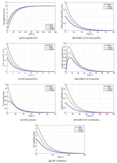
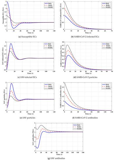
First strategy (Stability of ${\mathsf{\Delta }}_0$): $({\xi }_V,{\xi }_P,{\eta }_Z,{\eta }_M)=(0.001,0.001,0.01,0.02)$. These values gives ${\Re }_1=0.0744<1$ and ${\Re }_2=0.1922<1$. It is shown in Figure 1 that the trajectories starting with initials IS(I)-IS(III) tend to the equilibrium, ${\mathsf{\Delta }}_0=(10,0,0,0,0,0,0)$. This supports the global stability results given in Theorem 1. In this strategy, both influenza and COVID-19 will be cleared. In fact, making ${\Re }_1\le 1$ and ${\Re }_2\le 1$ can be achieved in one or more of the following ways: (i) applying two antiviral drugs for blocking SARS-CoV-2 and IAV infections with drug efficacies of ${ϵ}_V$ and ${ϵ}_P$, respectively, where $0\le {ϵ}_V\le 1$ and $0\le {ϵ}_P\le 1$; then, the parameters ${\xi }_V$ and ${\xi }_P$ will be reduced to $(1-{ϵ}_V){\xi }_V$ and $(1-{ϵ}_P){\xi }_P$, respectively; (ii) applying two antiviral drugs for blocking the replication of SARS-CoV-2 and IAV with drug efficacies of ${\epsilon }_V$ and ${\epsilon }_P$, respectively, where $0\le {\epsilon }_V\le 1$ and $0\le {\epsilon }_P\le 1$. Then, the parameters ${\theta }_V$ and ${\theta }_P$ will be reduced to $(1-{\epsilon }_V){\theta }_V$ and $(1-{\epsilon }_P){\theta }_P$, respectively.

Figure 1. Solutions of system (1)–(7) when ${\Re }_1\le 1$ and ${\Re }_2\le 1$ (first strategy).

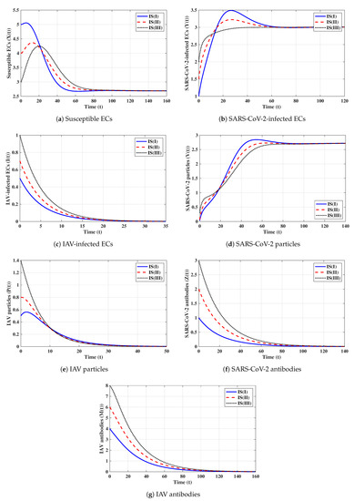
Second strategy (Stability of ${\mathsf{\Delta }}_1$): $({\xi }_V,{\xi }_P,{\eta }_Z,{\eta }_M)=(0.05,0.001,0.002,0.02)$. This selection provides ${\Re }_1=3.7215>1$, ${\Re }_3=0.1431<1$, and ${\Re }_2/{\Re }_1=0.0516<1$. The equilibrium ${\mathsf{\Delta }}_1$ exists with ${\mathsf{\Delta }}_1=(2.69,3.008,0,2.72,0,0,0)$. Figure 2 shows that the trajectories initiated with IS(I)-IS(III) converge to ${\mathsf{\Delta }}_1$, and this result agrees with Theorem 2. This strategy suggests that a COVID-19 mono-infection with an inactive antibody response will be established.

Figure 2. Solutions of system (1)–(7) when ${\Re }_1>1,{\Re }_2/{\Re }_1\le 1$, and ${\Re }_3\le 1$ (second strategy).

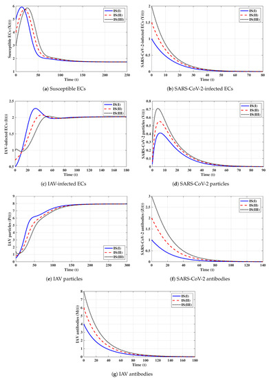
Third strategy (Stability of ${\mathsf{\Delta }}_2$): $({\xi }_V,{\xi }_P,{\eta }_Z,{\eta }_M)=(0.005,0.03,0.01,0.001)$. This gives ${\Re }_2=5.7647>1$, ${\Re }_4=0.2306<1$, and ${\Re }_1/{\Re }_2=0.0646<1$. The numerical solution confirms that ${\mathsf{\Delta }}_2=\left(1.73,0,2.03,0,7.94,0,0\right)$ exists. It can be observed from Figure 3 that the solutions initiated with IS(I)-IS(III) converge to ${\mathsf{\Delta }}_2$, and this result agrees with Theorem 3. This strategy suggests that an influenza mono-infection with an inactive antibody response will be established.

Figure 3. Solutions of system (1)–(7) when ${\Re }_2>1,{\Re }_1/{\Re }_2\le 1$, and ${\Re }_4\le 1$ (third strategy).

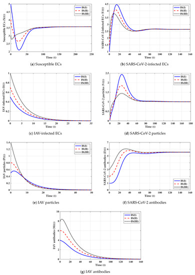
Fourth strategy (Stability of ${\mathsf{\Delta }}_3$): $({\xi }_V,{\xi }_P,{\eta }_Z,{\eta }_M)=(0.09,0.002,0.05,0.05)$. This yields ${\Re }_3=2.3924>1$ and ${\Re }_5=0.1373<1$. Figure 4 illustrates that the solutions tend to ${\mathsf{\Delta }}_3=(3.57,2.64,0,1,0,5.57,0)$ regardless of the initial states. This result supports the global stability result given in Theorem 4. This strategy shows that a COVID-19 mono-infection with an activated SARS-CoV-2-specific antibody response will be attained.

Figure 4. Solutions of system (1)–(7) when ${\Re }_3>1$ and ${\Re }_5\le 1$ (fourth strategy).

Fifth strategy (Stability of ${\mathsf{\Delta }}_4$): $({\xi }_V,{\xi }_P,{\eta }_Z,{\eta }_M)=(0.01,0.1,0.01,0.02)$. The values of ${\Re }_4$ and ${\Re }_6$ are computed as ${\Re }_4=3.8432>1$ and ${\Re }_6=0.1489<1$. Thus, ${\mathsf{\Delta }}_4$ exists with ${\mathsf{\Delta }}_4=(2,0,1.96,0,2,0,7.11)$. The numerical solutions with initials IS(I)-IS(III) tend to ${\mathsf{\Delta }}_4$ (see Figure 5). This shows the global stability of ${\mathsf{\Delta }}_4$ given in Theorem 5. In this strategy, an influenza mono-infection with a stimulated IAV-specific antibody response will be achieved.

Figure 5. Solutions of system (1)–(7) when ${\Re }_4>1$ and ${\Re }_6\le 1$ (fifth strategy).

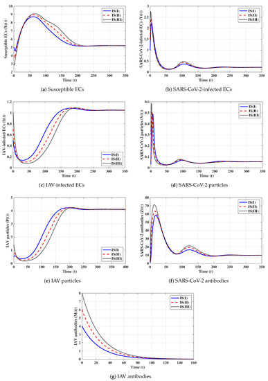
Sixth strategy (Stability of ${\mathsf{\Delta }}_5$): $({\xi }_V,{\xi }_P,{\eta }_Z,{\eta }_M)=(0.09,0.01,0.9,0.001)$. Then, we calculate ${\Re }_5=1.7469>1$, ${\Re }_8=0.2112<1$, and ${\Re }_1/{\Re }_2=3.486>1$. The numerical results displayed in Figure 6 establish that ${\mathsf{\Delta }}_5=(5.2,0.21,1.05,0.06,4.11,9.94,0)$ exists and that it is GAS; this agrees with the result of Theorem 6. This result suggests that a co-infection with influenza and COVID-19 with only an active SARS-CoV-2-specific antibody response will be attained.

Figure 6. Solutions of system (1)–(7) when ${\Re }_5>1,{\Re }_1/{\Re }_2>1$, and ${\Re }_8\le 1$ (sixth strategy).

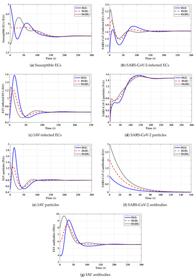
Seventh strategy (Stability of ${\mathsf{\Delta }}_6$): $({\xi }_V,{\xi }_P,{\eta }_Z,{\eta }_M)=(0.04,0.05,0.01,0.05)$. We compute ${\Re }_6=1.654>1$, ${\Re }_7=0.5133<1$, and ${\Re }_2/{\Re }_1=3.2272>1$. We find that the equilibrium ${\mathsf{\Delta }}_6=\left(3.36,1.63,0.66,1.47,0.8,0,5.57\right)$ exists. Figure 7 draws the numerical solutions of the DDEs with initials IS(I)-IS(III). It is shown that ${\mathsf{\Delta }}_6$ is GAS, and this supports the result of Theorem 7. This strategy leads to a co-infection with influenza and COVID-19 with only an active IAV-specific antibody response.

Figure 7. Solutions of system (1)–(7) when ${\Re }_6>1,{\Re }_2/{\Re }_1>1$, and ${\Re }_7\le 1$ (seventh strategy).

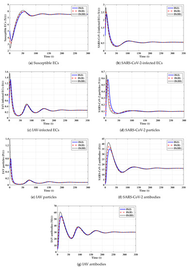
Eighth strategy 8 (Stability of ${\mathsf{\Delta }}_7$): $({\xi }_V,{\xi }_P,{\eta }_Z,{\eta }_M)=(0.09,0.09,0.5,0.5)$. This selection gives ${\Re }_7=5.0594>1$ and ${\Re }_8=13.0621>1$. Figure 8 shows that ${\mathsf{\Delta }}_7=(7.55,0.56,0.27,0.1,0.08,16.24,30.16)$ exists and that it is GAS according to Theorem 8. This strategy leads to the case of co-infection with influenza and COVID-19 in which both types of antibody responses are active.

Figure 8. Solutions of system (1)–(7) when ${\Re }_7>1$ and ${\Re }_8>1$ (eighth strategy).

6.2. Effect of Antiviral Treatment on the Dynamics of Influenza and COVID-19 Co-Infection

We consider two antiviral drugs for SARS-CoV-2 and IAV with drug efficacies of ${ϵ}_V$ and ${ϵ}_P$, respectively, where $0\le {ϵ}_V\le 1$ and $0\le {ϵ}_P\le 1$. Then, the parameters ${\xi }_V$ and ${\xi }_P$ will be changed to $(1-{ϵ}_V){\xi }_V$ and $(1-{ϵ}_P){\xi }_P$, respectively. Moreover, ${\Re }_1$ and ${\Re }_2$ become functions of ${ϵ}_V$ and ${ϵ}_P$, respectively, when all other parameters are fixed:

$${\Re }_1\left({ϵ}_V\right)=\frac{(1-{ϵ}_V)e^{-{\alpha }_1{\tau }_1-{\alpha }_2{\tau }_2}{X}_0{\theta }_V{\xi }_V}{{\lambda }_V{\beta }_Y},{\Re }_2\left({ϵ}_P\right)=\frac{(1-{ϵ}_P)e^{-{\alpha }_3{\tau }_3-{\alpha }_4{\tau }_4}{X}_0{\theta }_P{\xi }_P}{{\lambda }_P{\beta }_I}.$$

To make ${\Re }_1\le 1$ and ${\Re }_2\le 1$, the effectiveness of ${ϵ}_V$ and ${ϵ}_P$ has to satisfy

$$\begin{array}{cc}\hfill {ϵ}_V^{min}& \le {ϵ}_V\le 1,{ϵ}_V^{min}=max\left\{0,1-\frac{e^{{\alpha }_1{\tau }_1+{\alpha }_2{\tau }_2}{\lambda }_V{\beta }_Y}{X_0{\theta }_V{\xi }_V}\right\},\hfill \\ \hfill {ϵ}_P^{min}& \le {ϵ}_P\le 1,{ϵ}_P^{min}=max\left\{0,1-\frac{e^{{\alpha }_3{\tau }_3+{\alpha }_4{\tau }_4}{\lambda }_P{\beta }_I}{X_0{\theta }_P{\xi }_P}\right\}.\hfill \end{array}$$

It follows that, if ${ϵ}_V^{min}\le {ϵ}_V\le 1$ and ${ϵ}_P^{min}\le {ϵ}_P\le 1$, then ${\mathsf{\Delta }}_0$ is GAS, and both influenza and COVID-19 are cleared. Therefore, if real data from patients co-infected with influenza and COVID-19 are used, the model’s parameters can be estimated and the model can be used to determine the minimum drug efficacies required to eliminate both SARS-CoV-2 and IAV from the body.

6.3. Effects of Time Delays on the Dynamics of Influenza and COVID-19 Co-Infection

In this subsection, we analyze the impacts of time delays with various delay parameters ${\tau }_i,$$i=1,2,3,4$. We fix the parameters ${\xi }_V=0.13$, ${\xi }_P=0.1,$${\eta }_Z=0.3$, and ${\eta }_M=0.5$. Let us consider the following scenarios:

$$\begin{array}{ccccc}\hfill \mathrm{S}1:& {\tau }_1=0.1,\hfill & {\tau }_2=0.3,\hfill & {\tau }_3=0.5,\hfill & {\tau }_4=0.8,\hfill \\ \hfill \mathrm{S}2:& {\tau }_1=1,\hfill & {\tau }_2=0.9,\hfill & {\tau }_3=13,\hfill & {\tau }_4=14,\hfill \\ \hfill \mathrm{S}3:& {\tau }_1=1.2348,\hfill & {\tau }_2=1.2348,\hfill & {\tau }_3=14.9787,\hfill & {\tau }_4=14.9787,\hfill \\ \hfill \mathrm{S}4:& {\tau }_1=3,\hfill & {\tau }_2=4,\hfill & {\tau }_3=20,\hfill & {\tau }_4=25.\hfill \end{array}$$

From the above values, we solve the system (1)–(7) under the following initial condition:

$$\begin{array}{ccc}\hfill \mathrm{IS}\left(\mathrm{IV}\right)& :& (X\left(u\right),Y\left(u\right),I\left(u\right),V\left(u\right),P\left(u\right),Z\left(u\right),M\left(u\right))=\left(7,0.6,0.5,0.05,0.05,7,8\right),\hfill \\ \hfill u& \in & \left[-{\tau }^{*},0\right].\hfill \end{array}$$

The numerical results are displayed in Figure 9. We note that time delays can significantly increase the concentration of susceptible ECs and reduce the concentrations of other factors. Since ${\Re }_1$ and ${\Re }_2$ are given in (16), they depend on ${\tau }_i,$$i=1,2,3,4$ when all other parameters are fixed. We observe from Table 3 that ${\Re }_1$ and ${\Re }_2$ decrease if ${\tau }_i$ increases; hence, the stability of ${\mathsf{\Delta }}_0$ will be changed.

Figure 9. Effects of delay parameters ${\tau }_i,$$i=1,2,3,4$, on the trajectories of system (1)–(7).

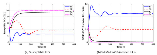
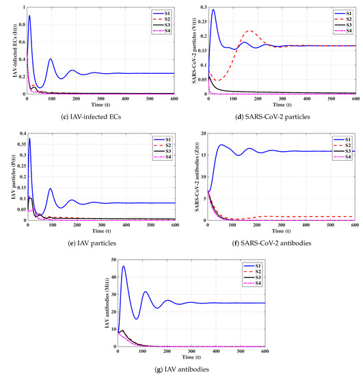
Table 3. The variation in ${\Re }_1$ and ${\Re }_2$ with respect to the delay parameters.

Delay Parameters	${\mathit{\Re }}_1$	${\mathit{\Re }}_2$
${\tau }_1=0.1,{\tau }_2=0.3,{\tau }_3=0.5$ and ${\tau }_4=0.8$	$7.92$	$17.56$
${\tau }_1=0.5,{\tau }_2=0.6,{\tau }_3=10$ and ${\tau }_4=11$	$3.93$	$2.45$
${\tau }_1=1,$${\tau }_2=0.9,$${\tau }_3=13$ and ${\tau }_4=14,$	$1.77$	$1.34$
${\tau }_1={\tau }_2=1.2348$ and ${\tau }_3={\tau }_4=14.9787,$	$1.0$	$1.0$
${\tau }_1=2,$${\tau }_2=3,$${\tau }_3=15$ and ${\tau }_4=16$	$0.08$	$0.9$
${\tau }_1=3,$${\tau }_2=4,$${\tau }_3=20$ and ${\tau }_4=25.$	$0.011$	$0.22$

Now, we need to calculate the critical value of the time delays that makes the system stable around the equilibrium point ${\mathsf{\Delta }}_0$. Let ${\tau }_{12}={\tau }_1={\tau }_2$ and ${\tau }_{34}={\tau }_3={\tau }_4,$ and we write ${\Re }_1\left({\tau }_{12}\right)$ and ${\Re }_2\left({\tau }_{34}\right)$ as:

$${\Re }_1\left({\tau }_{12}\right)=\frac{e^{-\left({\alpha }_1+{\alpha }_2\right){\tau }_{12}}{X}_0{\theta }_V{\xi }_V}{{\beta }_Y{\lambda }_V},{\Re }_2\left({\tau }_{34}\right)=\frac{e^{-\left({\alpha }_3+{\alpha }_4\right){\tau }_{34}}{X}_0{\theta }_P{\xi }_P}{{\beta }_I{\lambda }_P}.$$

Clearly, when all other parameters are fixed, ${\Re }_1$ and ${\Re }_2$ are decreasing functions of ${\tau }_{12}$ and ${\tau }_{34}$, respectively. Let us calculate ${\tau }_{12}^{min}$ and ${\tau }_{34}^{min}$ such that ${\Re }_1\left({\tau }_{12}^{min}\right)=1$ and ${\Re }_2\left({\tau }_{34}^{min}\right)=1$ as:

$$\begin{array}{cc}\hfill {\tau }_{12}^{min}& =max\left\{0,\frac{1}{{\alpha }_1+{\alpha }_2}ln\left(\frac{X_0{\theta }_V{\xi }_V}{{\beta }_Y{\lambda }_V}\right)\right\},\hfill \\ \hfill {\tau }_{34}^{min}& =max\left\{0,\frac{1}{{\alpha }_3+{\alpha }_4}ln\left(\frac{X_0{\theta }_P{\xi }_P}{{\beta }_I{\lambda }_P}\right)\right\}.\hfill \end{array}$$

Consequently,

$$\begin{array}{cc}\hfill {\Re }_1\left({\tau }_{12}\right)& \le 1,\mathrm{for}\mathrm{all}{\tau }_{12}\ge {\tau }_{12}^{min},\hfill \\ \hfill {\Re }_2\left({\tau }_{34}\right)& \le 1,\mathrm{for}\mathrm{all}{\tau }_{34}\ge {\tau }_{34}^{min}.\hfill \end{array}$$

Therefore, ${\mathsf{\Delta }}_0$ is GAS when ${\tau }_{12}\ge {\tau }_{12}^{min}$ and ${\tau }_{34}\ge {\tau }_{34}^{min}$. Using the values of the parameters, we get ${\tau }_{12}=1.2348$ and ${\tau }_{34}=14.9787$. It follows that:

(i) If ${\tau }_{12}\ge 1.2348$ and ${\tau }_{34}\ge 14.9787,$ then ${\Re }_1\left({\tau }_{12}\right)\le 1$, ${\Re }_2\left({\tau }_{34}\right)\le 1$, and ${\mathsf{\Delta }}_0$ is GAS.

(ii) If ${\tau }_{12}<1.2348$ or ${\tau }_{34}<14.9787,$ then ${\Re }_1\left({\tau }_{12}\right)>1$ or ${\Re }_2\left({\tau }_{34}\right)>1$, and ${\mathsf{\Delta }}_0$ will lose its stability.

We note that time delays can play a similar role to that of antiviral drugs. This can guide researchers to create new treatments for influenza and COVID-19 co-infection that work to prolong time delays.

7. Conclusions

Influenza and COVID-19 co-infection cases were reported in recent works (see, e.g., [5,9,10,11]). Mathematical models can be helpful for understanding the dynamics of influenza and COVID-19 co-infection within a host. In this paper, we developed and examined a system of DDEs to describe the in-host dynamics of influenza and COVID-19 co-infection under the effects of humoral immunity. The model considered the interactions among susceptible ECs, SARS-CoV-2-infected ECs, IAV-infected ECs, SARS-CoV-2 particles, IAV particles, SARS-CoV-2 antibodies, and IAV antibodies. The model included four time delays: ${\tau }_1$ and ${\tau }_3$ for the delays between the entries of SARS-CoV-2 and IAV into ECs and the start of production of immature SARS-CoV-2 and IAV virions, respectively, and ${\tau }_2$ and ${\tau }_4$ for the maturation delays of newly released SARS-CoV-2 and IAV virions, respectively. We showed the non-negativity and ultimate boundedness of the solutions. We deduced that the system had eight equilibria, and their existence and stability were governed by eight threshold parameters (${\Re }_i$, $i=1,2,\cdots ,8$). We used the Lyapunov method to prove the global stability of the equilibria. We carried out some numerical simulations and showed that they agreed with the theoretical results. We addressed the effects of antiviral drugs and time delays on the co-infection dynamics. We showed that both antiviral drugs and time delays had the same effect in eradicating co-infection from the body. This can guide scientists and pharmaceutical companies in synthesizing new drugs that prolong time delays. Our proposed model can be useful for determining the minimum drug doses that are required to eliminate both SARS-CoV-2 and IAV infections from the body. Moreover, the model can be used to describe the in-host dynamics of co-infection with two or more viral strains or co-infections with SARS-CoV-2 (or IAV) and other respiratory viruses.

The model presented in this article can be extended to include several biological aspects, such as viral mutation [61], stochastic interactions [62], and reaction diffusion [63].

References

- World Health Organization (WHO). Coronavirus Disease (COVID-19), Weekly Epidemiological Update (18 December 2022). 2022. Available online: https://www.who.int/publications/m/item/covid-19-weekly-epidemiological-update (accessed on 21 December 2022).
- Iuliano, A.D.; Roguski, K.M.; Chang, H.H.; Muscatello, D.J.; Palekar, R.; Tempia, S.; Cohen, C.; Gran, J.M.; Schanzer, D.; Cowling, N.J.; et al. Estimates of global seasonal influenza-associated respiratory mortality: A modelling study. Lancet 2018, 391, 1285–1300. [Google Scholar] [CrossRef] [PubMed]
- Hancioglu, B.; Swigon, D.; Clermont, G. A dynamical model of human immune response to influenza A virus infection. J. Theor. Biol. 2007, 246, 70–86. [Google Scholar] [CrossRef] [PubMed]
- Varga, Z.; Flammer, A.J.; Steiger, P.; Haberecker, M.; Andermatt, R.; Zinkernagel, A.S.; Mehra, M.P.; Schuepbach, R.A.; Ruschitzka, F.; Moch, H.; et al. Endothelial cell infection and endotheliitis in COVID-19. Lancet 2020, 395, 1417–1418. [Google Scholar] [CrossRef] [PubMed]
- Ozaras, R. Influenza and COVID-19 coinfection: Report of six cases and review of the literature. J. Med. Virol. 2020, 92, 2657–2665. [Google Scholar] [CrossRef]
- World Health Organization (WHO). Influenza Update No. 428, (19 September 2022). 2022. Available online: https://www.who.int/publications/m/item/influenza-update-n-428 (accessed on 21 December 2022).
- World Health Organization (WHO). Coronavirus Disease (COVID-19), Vaccine Tracker. 2022. Available online: https://covid19.trackvaccines.org/agency/who/ (accessed on 21 December 2022).
- Nuwarda, R.F.; Alharbi, A.A.; Kayser, V. An overview of influenza viruses and vaccines. Vaccines 2021, 9, 1032. [Google Scholar] [CrossRef]
- Zhu, X.; Ge, Y.; Wu, T.; Zhao, K.; Chen, Y.; Wu, B.; Zhu, F.; Zhu, B.; Cui, L. Co-infection with respiratory pathogens among COVID-2019 cases. Virus Res. 2020, 285, 198005. [Google Scholar] [CrossRef]
- Ding, Q.; Lu, P.; Fan, Y.; Xia, Y.; Liu, M. The clinical characteristics of pneumonia patients coinfected with 2019 novel coronavirus and influenza virus in Wuhan, China. J. Med. Virol. 2020, 92, 1549–1555. [Google Scholar] [CrossRef]
- Wang, G.; Xie, M.; Ma, J.; Guan, J.; Song, Y.; Wen, Y.; Fang, D.; Wang, M.; Tian, D.-a.; Li, P.; et al. Is Co-Infection with Influenza Virus a Protective Factor of COVID-19? 2020. Available online: https://papers.ssrn.com/sol3/papers.cfm?abstract_id=3576904 (accessed on 21 December 2022).
- Wang, M.; Wu, Q.; Xu, W.; Qiao, B.; Wang, J.; Zheng, H.; Jiang, S.; Mei, J.; Wu, Z.; Deng, Y.; et al. Clinical diagnosis of 8274 samples with 2019-novel coronavirus in Wuhan. MedRxiv 2020. [Google Scholar] [CrossRef]
- Lansbury, L.; Lim, B.; Baskaran, V.; Lim, W.S. Co-infections in people with COVID-19: A systematic review and meta-analysis. J. Infect. 2020, 81, 266–275. [Google Scholar] [CrossRef]
- Ghaznavi, H.; Shirvaliloo, M.; Sargazi, S.; Mohammadghasemipour, Z.; Shams, Z.; Hesari, Z.; Shahraki, O.; Nazarlou, Z.; Sheervalilou, R.; Shirvalilou, S. SARS-CoV-2 and influenza viruses: Strategies to cope with coinfection and bioinformatics perspective. Cell Biol. Int. 2022, 46, 1009–1020. [Google Scholar] [CrossRef]
- Khorramdelazad, H.; Kazemi, M.H.; Najafi, A.; Keykhaee, M.; Emameh, R.Z.; Falak, R. Immunopathological similarities between COVID-19 and influenza: Investigating the consequences of co-infection. Microb. Pathog. 2021, 152, 104554. [Google Scholar] [CrossRef] [PubMed]
- Xiang, X.; Wang, Z.H.; Ye, L.L.; He, X.L.; Wei, X.S.; Ma, Y.L.; Li, H.; Chen, L.; Wang, X.-r.; Zhou, Q. Co-infection of SARS-COV-2 and influenza A virus: A case series and fast review. Curr. Med. Sci. 2021, 41, 51–57. [Google Scholar] [CrossRef]
- Nowak, M.D.; Sordillo, E.M.; Gitman, M.R.; Mondolfi, A.E.P. Coinfection in SARS-CoV-2 infected patients: Where are influenza virus and rhinovirus/enterovirus? J. Med. Virol. 2020, 92, 1699. [Google Scholar] [CrossRef]
- Pinky, L.; Dobrovolny, H.M. SARS-CoV-2 coinfections: Could influenza and the common cold be beneficial? J. Med. Virol. 2020, 92, 2623–2630. [Google Scholar] [CrossRef]
- Pinky, L.; Dobrovolny, H.M. Coinfections of the respiratory tract: Viral competition for resources. PLoS ONE 2016, 11, e0155589. [Google Scholar] [CrossRef] [PubMed]
- Hashemi, S.A.; Safamanesh, S.; Ghasemzadeh-moghaddam, H.; Ghafouri, M.; Azimian, A. High prevalence of SARS-CoV-2 and influenza A virus (H1N1) coinfection in dead patients in Northeastern Iran. J. Med. Virol. 2021, 93, 1008–1012. [Google Scholar] [CrossRef]
- Smith, A.M.; Ribeiro, R.M. Modeling the viral dynamics of influenza A virus infection. Crit. Rev. Immunol. 2010, 30, 291–298. [Google Scholar] [CrossRef] [PubMed]
- Beauchemin, C.A.; Handel, A. A review of mathematical models of influenza A infections within a host or cell culture: Lessons learned and challenges ahead. BMC Public Health 2011, 11, S7. [Google Scholar] [CrossRef] [PubMed]
- Canini, L.; Perelson, A.S. Viral kinetic modeling: State of the art. J. Pharmacokinet. Pharmacodyn. 2014, 41, 431–443. [Google Scholar] [CrossRef] [PubMed]
- Handel, A.; Liao, L.E.; Beauchemin, C.A. Progress and trends in mathematical modelling of influenza A virus infections. Curr. Opin. Syst. Biol. 2018, 12, 30–36. [Google Scholar] [CrossRef]
- Baccam, P.; Beauchemin, C.; Macken, C.A.; Hayden, F.G.; Perelson, A. Kinetics of influenza A virus infection in humans. J. Virol. 2006, 80, 7590–7599. [Google Scholar] [CrossRef]
- Saenz, R.A.; Quinlivan, M.; Elton, D.; MacRae, S.; Blunden, A.S.; Mumford, J.A.; Daly, J.M.; Digard, P.; Cullinane, A.; Grenfell, B.T.; et al. Dynamics of influenza virus infection and pathology. J. Virol. 2010, 84, 3974–3983. [Google Scholar] [CrossRef] [PubMed]
- Lee, H.Y.; Topham, D.J.; Park, S.Y.; Hollenbaugh, J.; Treanor, J.; Mosmann, T.R.; Jin, X.; Ward, B.M.; Miao, H.; Holden-Wiltse, J.; et al. Simulation and prediction of the adaptive immune response to influenza A virus infection. J. Virol. 2009, 83, 7151–7165. [Google Scholar] [CrossRef]
- Tridane, A.; Kuang, Y. Modeling the interaction of cytotoxic T lymphocytes and influenza virus infected epithelial cells. MBE 2010, 7, 171–185. [Google Scholar] [PubMed]
- Hernandez-Vargas, E.A.; Wilk, E.; Canini, L.; Toapanta, F.R.; Binder, S.C.; Uvarovskii, A.; Ross, T.M.; Guzmán, C.A.; Perelson, A.S.; Meyer-Hermann, M. Effects of aging on influenza virus infection dynamics. J. Virol. 2014, 88, 4123–4131. [Google Scholar] [CrossRef] [PubMed]
- Li, K.; McCaw, J.M.; Cao, P. Modelling within-host macrophage dynamics in influenza virus infection. J. Theor. Biol. 2021, 508, 110492. [Google Scholar] [CrossRef] [PubMed]
- Chang, D.B.; Young, C.S. Simple scaling laws for influenza A rise time, duration, and severity. J. Theor. Biol. 2007, 246, 621–635. [Google Scholar] [CrossRef]
- Handel, A.; Longini, I.M., Jr.; Antia, R. Towards a quantitative understanding of the within-host dynamics of influenza A infections. J. R. Soc. Interface 2010, 7, 35–47. [Google Scholar] [CrossRef]
- Handel, A.; Longini, I.M., Jr.; Antia, R. Neuraminidase inhibitor resistance in influenza: Assessing the danger of its generation and spread. PLoS Comput. 2007, 3, e240. [Google Scholar] [CrossRef]
- Beauchemin, C.A.; McSharry, J.J.; Drusano, G.L.; Nguyen, J.T.; Went, G.T.; Ribeiro, R.M.; Perelson, A.S. Modeling amantadine treatment of influenza A virus in vitro. J. Theor. Biol. 2008, 254, 439–451. [Google Scholar] [CrossRef]
- Hernandez-Vargas, E.A.; Velasco-Hernandez, J.X. In-host mathematical modelling of COVID-19 in humans. Annu. Rev. Control 2020, 50, 448–456. [Google Scholar] [CrossRef] [PubMed]
- Li, C.; Xu, J.; Liu, J.; Zhou, Y. The within-host viral kinetics of SARS-CoV-2. MBE 2020, 17, 2853–2861. [Google Scholar] [CrossRef]
- Ke, R.; Zitzmann, C.; Ho, D.D.; Ribeiro, R.M.; Perelson, A.S. In vivo kinetics of SARS-CoV-2 infection and its relationship with a person’s infectiousness. Proc. Natl. Acad. Sci. USA 2021, 118, e2111477118. [Google Scholar] [CrossRef] [PubMed]
- Sadria, M.; Layton, A.T. Modeling within-host SARS-CoV-2 infection dynamics and potential treatments. Viruses 2021, 13, 1141. [Google Scholar] [CrossRef] [PubMed]
- Ghosh, I. Within host dynamics of SARS-CoV-2 in humans: Modeling immune responses and antiviral treatments. SN Comput. Sci. 2021, 2, 482. [Google Scholar] [CrossRef] [PubMed]
- Du, S.Q.; Yuan, W. Mathematical modeling of interaction between innate and adaptive immune responses in COVID-19 and implications for viral pathogenesis. J. Med. Virol. 2020, 92, 1615–1628. [Google Scholar] [CrossRef] [PubMed]
- Hattaf, K.; Yousfi, N. Dynamics of SARS-CoV-2 infection model with two modes of transmission and immune response. MBE 2020, 17, 5326–5340. [Google Scholar] [CrossRef]
- Mondal, J.; Samui, P.; Chatterjee, A.N. Dynamical demeanour of SARS-CoV-2 virus undergoing immune response mechanism in COVID-19 pandemic. Eur. Phys. J. Spec. Top. 2022, 231, 3357–3370. [Google Scholar] [CrossRef]
- Almoceraa, A.E.S.; Quiroz, G.; Hernandez-Vargas, E.A. Stability analysis in COVID-19 within-host model with immune response. CNSNS 2021, 95, 105584. [Google Scholar] [CrossRef]
- Leon, C.; Tokarev, A.; Bouchnita, A.; Volpert, V. Modelling of the innate and adaptive immune response to SARS viral infection, cytokine storm and vaccination. Vaccines 2023, 11, 127. [Google Scholar] [CrossRef]
- Gonçalves, A.; Bertr, J.; Ke, R.; Comets, E.; De Lamballerie, X.; Malvy, D.; Pizzorno, A.; Terrier, O.; Calatrava, M.R.; Mentré, F.; et al. Timing of antiviral treatment initiation is critical to reduce SARS-CoV-2 viral load. CPT Pharmacomet. Syst. Pharmacol. 2020, 9, 509–514. [Google Scholar] [CrossRef] [PubMed]
- Abuin, P.; Anderson, A.; Ferramosca, A.; Hernandez-Vargas, E.A.; Gonzalez, A.H. Characterization of SARS-CoV-2 dynamics in the host. Annu. Rev. Control 2020, 50, 457–468. [Google Scholar] [CrossRef] [PubMed]
- Chhetri, B.; Bhagat, V.M.; Vamsi, D.K.K.; Ananth, V.S.; Prakash, D.B.; Mandale, R.; Muthusamy, S.; Sanjeevi, C.B. Within-host mathematical modeling on crucial inflammatory mediators and drug interventions in COVID-19 identifies combination therapy to be most effective and optimal. Alex. Eng. J. 2021, 60, 2491–2512. [Google Scholar] [CrossRef]
- Elaiw, A.M.; Alsaedi, A.J.; Agha, A.D.A.; Hobiny, A.D. Global stability of a humoral immunity COVID-19 model with logistic growth and delays. Mathematics 2022, 10, 1857. [Google Scholar] [CrossRef]
- Mahiout, L.A.; Bessonov, N.; Kazmierczak, B.; Volpert, V. Mathematical modeling of respiratory viral infection and applications to SARS-CoV-2 progression. Math. Methods Appl. Sci. 2023, 46, 1740–1751. [Google Scholar] [CrossRef]
- dePillis, L.; Caffrey, R.; Chen, G.; Dela, M.D.; Eldevik, L.; McConnell, J.; Shabahang, S.; Varvel, S.A. A mathematical model of the within-host kinetics of SARS-CoV-2 neutralizing antibodies following COVID-19 vaccination. J. Theor. Biol. 2023, 556, 111280. [Google Scholar] [CrossRef]
- Nath, B.J.; Dehingia, K.; Mishra, V.N.; Chu, Y.-M.; Sarmah, H.K. Mathematical analysis of a within-host model of SARS-CoV-2. Adv. Differ. Equ. 2021, 2021, 113. [Google Scholar] [CrossRef]
- Hattaf, K.; Karimi, E.; Ismail, M.; Mohsen, A.A.; Hajhouji, Z.; El Younoussi, M.; Yousfi, N. Mathematical modeling and analysis of the dynamics of RNA viruses in presence of immunity and treatment: A case study of SARS-CoV-2. Vaccines 2023, 11, 201. [Google Scholar] [CrossRef]
- Elaiw, A.M.; Alsulami, R.S.; Hobiny, A.D. Modeling and stability analysis of within-host IAV/SARS-CoV-2 coinfection with antibody immunity. Mathematics 2022, 10, 4382. [Google Scholar] [CrossRef]
- Elaiw, A.M.; Alsulami, R.S.; Hobiny, A.D. Global dynamics of IAV/SARS-CoV-2 coinfection model with eclipse phase and antibody immunity. Math. Biosci. Eng. 2023, 20, 3873–3917. [Google Scholar] [CrossRef]
- Hale, J.K.; Lunel, S.V. Introduction to Functional Differential Equations; Springer Science & Business Media: New York, NY, USA, 1993. [Google Scholar]
- Korobeinikov, A. Global properties of basic virus dynamics models. Bull. Math. Biol. 2004, 66, 879–883. [Google Scholar] [CrossRef] [PubMed]
- Korobeinikov, A. Global properties of infectious disease models with nonlinear incidence. Bull. Math. Biol. 2007, 69, 1871–1886. [Google Scholar] [CrossRef] [PubMed]
- Barbashin, E.A. Introduction to the Theory of Stability; Wolters-Noordhoff: Groningen, The Netherlands, 1970. [Google Scholar]
- LaSalle, J.P. The Stability of Dynamical Systems; SIAM: Philadelphia, PA, USA, 1976. [Google Scholar]
- Lyapunov, A.M. The General Problem of the Stability of Motion; Taylor & Francis Ltd.: London, UK, 1992. [Google Scholar]
- Bellomo, N.; Burini, D.; Outada, N. Pandemics of mutating virus and society: A multi-scale active particles approach. Philos. Trans. A Math. Phys. Eng. Sci. 2022, 380, 20210161. [Google Scholar] [CrossRef] [PubMed]
- Gibelli, L.; Elaiw, A.M.; Alghamdi, M.A.; Althiabi, A.M. Heterogeneous population dynamics of active particles: Progression, mutations, and selection dynamics. Math. Model. Methods Appl. Sci. 2017, 27, 617–640. [Google Scholar] [CrossRef]
- Bellomo, N.; Outada, N.; Soler, J.; Tao, Y.; Winkler, M. Chemotaxis and cross diffusion models in complex environments: Modeling towards a multiscale vision. Math. Model. Methods Appl. Sci. 2022, 32, 713–792. [Google Scholar] [CrossRef]
Disclaimer/Publisher’s Note: The statements, opinions and data contained in all publications are solely those of the individual author(s) and contributor(s) and not of MDPI and/or the editor(s). MDPI and/or the editor(s) disclaim responsibility for any injury to people or property resulting from any ideas, methods, instructions or products referred to in the content. |
© 2023 by the authors. Licensee MDPI, Basel, Switzerland. This article is an open access article distributed under the terms and conditions of the Creative Commons Attribution (CC BY) license (https://creativecommons.org/licenses/by/4.0/).