Direct Power Series Approach for Solving Nonlinear Initial Value Problems

Abstract

In this research, a new approach for solving fractional initial value problems is presented. The main goal of this study focuses on establishing direct formulas to find the coefficients of approximate series solutions of target problems. The new method provides analytical series solutions for both fractional and ordinary differential equations or systems directly, without complicated computations. To show the reliability and efficiency of the presented technique, interesting examples of systems and fractional linear and nonlinear differential equations of ordinary and fractional orders are presented and solved directly by the new approach. This new method is faster and better than other analytical methods in establishing many terms of analytic solutions. The main motivation of this work is to introduce general new formulas that express the series solutions of some types of differential equations in a simple way and with less calculations compared to other numerical power series methods, that is, there is no need for differentiation, discretization, or taking limits while constructing the approximate solution.

1. Introduction

Fractional calculus is a generalization of classical calculus that studies integrals and derivatives of a non-integer order. Many definitions of FC have been introduced by scientists such as Leibniz, Liouville, Riemann, Grunwald, and Michele Caputo. More details on FC theories and applications can be found in [1,2,3,4,5,6]. Recently, many studies have been published that use the fractional derivative in modeling and analyzing new problems in various branches of science such as mathematical physics and engineering [7,8,9].

There are different methods for solving fractional differential equations. One of them is the residual power series method (RPSM), an efficient analytical technique for treating different types of fractional differential equations and systems. It is based on the generalized Taylor series formula and uses the power series for the functions, which gives an analytical series solution in the form of a convergent series [10,11,12,13,14]. On the other hand, researchers have invented many new methods based on the RPSM, and some of them combine the Laplace transform with the RPSM to obtain the Laplace residual power series method, while others use the Laplace transform with the idea of a power series and others, as in [15,16,17,18,19,20]. Recently, new transformations have been used to solve fractional differential equations, as in [20,21,22,23,24,25,26,27,28]. All these methods provide analytical series solutions to initial value problems, but the techniques differ between them [29,30,31].

In this article, we introduce the direct power series method (DPSM), which is a new numerical method that does not require integral transformations or differentiation. This new technique solves linear and nonlinear ordinary and fractional differential equations. It saves researchers effort and time in determining the coefficients of the analytical series expansions obtained through their work. It provides reliable and efficient solutions compared to other methods. This method depends on simple substitutions made on a target equation or system of differential equations that directly compute the coefficients of the power series expansion for the unknown functions. Furthermore, the substitutions in this article solve some time-fractional differential equations or systems that can be solved by power series methods. In addition, researchers can discover a new mathematical playground with this method.

In literature, there are many analytical and approximate methods for solving fractional differential equations, such as [32,33,34]. All of these techniques require long computations and efforts. With DPSM, we do not require these complicated operations, such as differentiation, discretization, and others, and we can find a general term of the solution directly with simple replacements. The novelty of this work is precisely obvious in the proposed method and its speediness and simplicity in presenting analytical series solutions that converge rapidly to the exact ones. The strength of DPSM is its ability to be programmed and provide many terms of a series solution in comparison to other numerical methods. DPSM can help researchers study the series solutions of new equations and systems with less time and effort spent computing approximate solutions using other methods.

In addition, many illustrative examples have been solved by DPSM. These examples have previously been solved by other numerical methods in the literature, and we achieve the same results faster. Further, other methods were too difficult to apply or took a long time to arrive at the solution; however, with DPSM, the steps to identify the solutions are fully shown and the calculations with software are even easier than the calculations for other power series methods.

This article is structured as follows: The second section illustrates preliminary information about FC. The main theorem of this research, and the steps of DPSM, are presented in section three. Finally, numerical examples and figures are presented in the fourth section.

2. Preliminaries

In this section, important definitions and properties of FC are presented. In addition, definitions and theorems of the fractional power series are introduced, which can be found in [10,11,12,13,14,15].

Definition 1. 

The Caputo fractional derivative operator of order α of the function$y\left(t\right)$, is defined by

$$D^{\alpha }\left[y\left(t\right)\right]=\{\begin{array}{c}\frac{1}{\Gamma \left(n-\alpha \right)}{{\displaystyle \int }}_0^t\frac{y^{\left(m\right)}\left(\xi \right)}{{\left(t-\xi \right)}^{\alpha +1-m}}d\xi , m-1<\alpha <m, m\in \mathbb{N}.\\ \frac{d^m}{d{t}^m}y\left(t\right), \alpha =m.\end{array}$$

(1)

Lemma 1. 

The following properties are important for Caputo definition

i.	$D^{\alpha }c=0$ ( $c$ is an arbitrary constant), $m-1<\alpha \le m$, $m\in \mathbb{N}$.
ii.	$D^{\alpha }{t}^{\beta }=\frac{\mathsf{\Gamma }\left(\mathsf{\beta }+1\right)}{\mathsf{\Gamma }\left(\beta +1-\alpha \right)}{t}^{\beta -\alpha },m-1<\alpha <m, \beta >m-1, m, n\in \mathbb{N}, \beta \in ℝ.$
iii.	$D^{k\alpha }{t}^{n\alpha }=\{\begin{array}{c}\frac{\mathsf{\Gamma }\left(n\mathsf{\alpha }+1\right)}{\mathsf{\Gamma }\left(\left(n-k\right)\alpha +1\right)}{t}^{\left(n-k\right)\alpha }, n\ge k\hfill \\ 0 , n<k\end{array},m-1<\alpha <m, k,m,n\in \mathbb{N}.$
iv.	$D^{k\alpha }\left({\displaystyle {\displaystyle \sum }_{n=0}^{\infty }}\frac{a_n{\left(\gamma t\right)}^{n\alpha }}{\mathsf{\Gamma }\left(n\alpha +1\right)}\right)={\displaystyle {\displaystyle \sum }_{n=0}^{\infty }}\frac{{\gamma }^{\left(n+k\right)\alpha }{a}_{n+k}{t}^{n\alpha }}{\mathsf{\Gamma }\left(n\alpha +1\right)}, m-1<\alpha <m, m,k,n\in \mathbb{N}.$

The following two theorems introduce a fractional power series representation and some related convergence analysis.

Theorem 1 [11]. 

Suppose that $y\left(t\right)$has a fractional power series representation at $t_0=0$, of the form

$$y\left(t\right)={\displaystyle \sum }_{n=0}^{\infty }\frac{a_n{t}^{n\alpha }}{\Gamma \left(n\alpha +1\right)},$$

(2)

where $m-1<\alpha \le m$ and $0\le t<R$, $m\in \mathbb{N},$ and $R\in ℝ$, where $R$ is the radius of convergence. If $D^{n\alpha }y\left(t\right)$ is continuous on $\left(0, R\right),$ then the coefficients of the equation $a_n$ and $\forall n=0, 1, \dots$ are given by:

$$a_n=D_t^{n\alpha }y\left(0\right).$$

(3)

Theorem 2 [11]. 

There are three cases for the convergence of the fractional power series ${\displaystyle \sum }_{n=0}^{\infty }\frac{a_n{t}^{n\alpha }}{\Gamma \left(n\alpha +1\right)}$as bellow

• For $t=0$, the series converges and the radius of convergence is equal to zero.
• For all $t\ge 0$, the series converges and the radius of convergence is equal to $\infty$.
• For $0\le t\le R$, the series converges, and for $t>R$, the series diverges where $R$ is a positive real number. Herein, $R$ is radius of convergence for the fractional power series.

3. Algorithm of DPSM

Numerical methods, such as the power series methods, are approximate techniques used to find numerical solutions to difficult problems such as nonlinear differential equations. The main idea of the power series approach, depends on expressing the solution in a form of an infinite series, and obtaining the series coefficients. Hence, to obtain efficient approximate solutions, we should find many terms (coefficients) of the series expansion.

In this section, we present a new technique, DPSM, which could be used to solve linear and nonlinear differential equations of ordinary or fractional order and systems. We present the main theorem in this new approach, that states the replacements that should be made in using the DPSM.

3.1. Main Theorem in DPSM

The following theorem presents the main theorem of DPSM in which we introduce the main replacements that will be applied to the target equations to apply the new method.

Theorem 3. 

Suppose that $y\left(t\right)$and $f\left(t\right)$have the fractional power series representations, such as

$$y\left(t\right)={\displaystyle \sum }_{n=0}^{\infty }\frac{a_n{t}^{n\alpha }}{\Gamma \left(n\alpha +1\right)} \mathrm{and} f\left(t\right)={\displaystyle \sum }_{m=0}^{\infty }\frac{b_m{t}^{m\alpha }}{\Gamma \left(m\alpha +1\right)},$$

where $y\left(t\right)$ and $f\left(t\right)$ are analytical functions, and $a_n$, $b_m$ are the coefficients of $\frac{t^{n\alpha }}{\Gamma \left(n\alpha +1\right)}$ and $\frac{t^{m\alpha }}{\Gamma \left(m\alpha +1\right)}$ for the functions $y\left(t\right)$ and $f\left(t\right),$ respectively. Then, $\forall n=0, 1,\cdots$ and $m=0,1,2,\cdots$, and then we can determine:

(i)	$a_{n+k}$ is the coefficient of $\frac{t^{n\alpha }}{\mathsf{\Gamma }\left(n\alpha +1\right)}$ in the series expansion of $D^{k\alpha }y\left(t\right)$ for any $k=0, 1, \cdots$.
(ii)	${\gamma }^{\left(n+k\right)\alpha }{a}_{n+k}$ is the coefficient of $\frac{t^{n\alpha }}{\mathsf{\Gamma }\left(n\alpha +1\right)}$ in the series expansion of $D^{k\alpha }y\left(\gamma t\right)$ for any $k=0, 1, \cdots$ and $\gamma \in ℝ$.
(iii)	${\displaystyle {\displaystyle \sum }_{i=0}^n}\frac{a_i{b}_{n-i}\mathsf{\Gamma }\left(n\alpha +1\right)}{\mathsf{\Gamma }\left(i\alpha +1\right)\mathsf{\Gamma }\left(\left(n-i\right)\alpha +1\right)}\mathrm{is} \mathrm{the} \mathrm{coefficient} \mathrm{of} \frac{t^{n\alpha }}{\mathsf{\Gamma }\left(n\alpha +1\right)} \mathrm{in} \mathrm{the} \mathrm{series}$ $\mathrm{expansion} \mathrm{of} y\left(t\right)f\left(t\right).$
(iv)	${\displaystyle {\displaystyle \sum }_{i=0}^n}\frac{{\beta }^{i\alpha }{\gamma }^{\left(n-i\right)\alpha }{a}_i{b}_{n-i}\mathsf{\Gamma }\left(n\alpha +1\right)}{\mathsf{\Gamma }\left(i\alpha +1\right)\mathsf{\Gamma }\left(\left(n-i\right)\alpha +1\right)}\mathrm{is} \mathrm{the} \mathrm{coefficient} \mathrm{of} \frac{t^{n\alpha }}{\mathsf{\Gamma }\left(n\alpha +1\right)} \mathrm{in} \mathrm{the} \mathrm{series}$ $\mathrm{expansion} \mathrm{of} y\left(\beta \mathrm{t}\right)f\left(\mathsf{\gamma }\mathrm{t}\right), \mathrm{where} \beta \mathrm{and} \gamma \in ℝ.$
(v)	${\displaystyle {\displaystyle \sum }_{i=0}^n}\frac{{\beta }^{\left(i+k\right)\alpha }{\gamma }^{\left(n-i+m\right)\alpha }{a}_{i+k}{b}_{n-i+m}\Gamma \left(n\alpha +1\right)}{\Gamma \left(i\alpha +1\right)\Gamma \left(\left(n-i\right)\alpha +1\right)}\mathrm{is} \mathrm{the} \mathrm{coefficient} \mathrm{of}\frac{t^{n\alpha }}{\mathsf{\Gamma }\left(n\alpha +1\right)} \mathrm{in} \mathrm{the}$ $\mathrm{series} \mathrm{expansion} \mathrm{of} D^{k\alpha }y\left(\mathsf{\beta }\mathrm{t}\right)D^{m\alpha }f\left(\mathsf{\gamma }\mathrm{t}\right), \mathrm{where} \beta$,$\gamma \in ℝ, \mathrm{and} \forall k=0, 1, \cdots .$

Proof of (i). 

Substituting the series expansion of $y\left(t\right)$ into $D^{k\alpha }y\left(t\right)$, we obtain

$$D^{k\alpha }y\left(t\right)=D^{k\alpha }\left({\displaystyle \sum }_{n=0}^{\infty }\frac{a_n{t}^{n\alpha }}{\Gamma \left(n\alpha +1\right)}\right).$$

□

Using part (iv) of Lemma 1, we obtain

$$D^{k\alpha }y\left(t\right)={\displaystyle \sum }_{n=k}^{\infty }\frac{a_n{t}^{\left(n-k\right)\alpha }}{\Gamma \left(\left(n-k\right)\alpha +1\right)}.$$

(4)

Thus, the series expansion (4) can be written as

$$D^{k\alpha }y\left(t\right)={\displaystyle \sum }_{n=0}^{\infty }\frac{a_{n+k}{t}^{n\alpha }}{\Gamma \left(n\alpha +1\right)}.$$

Proof of (ii). 

Substituting the series expansion of $y\left(\gamma t\right)$ into $D^{k\alpha }y\left(\gamma t\right)$, we obtain

$$D^{k\alpha }y\left(\gamma t\right)=D^{k\alpha }\left({\displaystyle \sum }_{n=0}^{\infty }\frac{a_n{\left(\gamma t\right)}^{n\alpha }}{\Gamma \left(n\alpha +1\right)}\right).$$

□

Using part (iv) of Lemma 1, we obtain

$$D^{k\alpha }y\left(\gamma t\right)={\displaystyle \sum }_{n=k}^{\infty }\frac{{\gamma }^{n\alpha }{a}_n{t}^{\left(n-k\right)\alpha }}{\Gamma \left(\left(n-k\right)\alpha +1\right)}.$$

(5)

Thus, Equation (5) can be written as

$$D^{k\alpha }y\left(\gamma t\right)={\displaystyle \sum }_{n=0}^{\infty }\frac{{\gamma }^{\left(n+k\right)\alpha }{a}_{n+k}{t}^{n\alpha }}{\Gamma \left(n\alpha +1\right)}.\mathsf{\Psi }$$

Proof of (iii). 

Multiplying the series expansion of $y\left(t\right) \mathrm{and} f\left(t\right)$, we obtain

$$y\left(t\right)f\left(t\right)=\left({\displaystyle \sum }_{i=0}^{\infty }\frac{a_i{t}^{i\alpha }}{\Gamma \left(i\alpha +1\right)}\right)\left({\displaystyle \sum }_{j=0}^{\infty }\frac{b_j{t}^{j\alpha }}{\Gamma \left(j\alpha +1\right)}\right).$$

(6)

□

Equation (6) can be simplified as

$$y\left(t\right)f\left(t\right)={\displaystyle \sum }_{i=0}^{\infty }{\displaystyle \sum }_{j=0}^{\infty }\frac{a_i{b}_j{t}^{\left(i+j\right)\alpha }}{\Gamma \left(i\alpha +1\right)\Gamma \left(j\alpha +1\right)},$$

which can be rewritten as

$$y\left(t\right)f\left(t\right)={\displaystyle \sum }_{n=0}^{\infty }\frac{\left({{\displaystyle \sum }}_{i=0}^n\frac{a_i{b}_{n-i}\Gamma \left(n\alpha +1\right)}{\Gamma \left(i\alpha +1\right)\Gamma \left(\left(n-i\right)\alpha +1\right)}\right)t^{n\alpha }}{\Gamma \left(n\alpha +1\right)}.\mathsf{\Psi }$$

Proof of (iv). 

Multiplying the series expansion of $y\left(\beta t\right) \mathrm{and} f\left(\gamma t\right)$, we obtain

$$y\left(\beta t\right)f\left(\gamma t\right)=\left({\displaystyle \sum }_{i=0}^{\infty }\frac{a_i{\left(\beta t\right)}^{i\alpha }}{\Gamma \left(i\alpha +1\right)}\right)\left({\displaystyle \sum }_{j=0}^{\infty }\frac{b_j{\left(\gamma t\right)}^{j\alpha }}{\Gamma \left(j\alpha +1\right)}\right).$$

(7)

□

Equation (7) can be written as

$$y\left(\beta t\right)f\left(\gamma t\right)={\displaystyle \sum }_{i=0}^{\infty }{\displaystyle \sum }_{j=0}^{\infty }\frac{a_i{b}_j{\beta }^{i\alpha }{\gamma }^{j\alpha }{t}^{\left(i+j\right)\alpha }}{\Gamma \left(i\alpha +1\right)\Gamma \left(j\alpha +1\right)},$$

which can be simplified as

$$y\left(\beta t\right)f\left(\gamma t\right)={\displaystyle \sum }_{n=0}^{\infty }\frac{\left({{\displaystyle \sum }}_{i=0}^n\frac{{\beta }^{i\alpha }{\gamma }^{\left(n-i\right)\alpha }{a}_i{b}_{n-i}\Gamma \left(n\alpha +1\right)}{\Gamma \left(i\alpha +1\right)\Gamma \left(\left(n-i\right)\alpha +1\right)}\right)t^{n\alpha }}{\Gamma \left(n\alpha +1\right)}.\mathsf{\Psi }$$

(8)

Proof of (v). 

Substituting the series expansion of $y\left(\beta t\right) \mathrm{and} f\left(\gamma t\right)$ into $D^{k\alpha }y\left(\beta t\right) D^{m\alpha }f\left(\gamma t\right)$, we obtain

$$D^{k\alpha }y\left(\beta t\right)D^{m\alpha }f\left(\gamma t\right)=D^{k\alpha }\left({\displaystyle \sum }_{i=0}^{\infty }\frac{a_i{\left(\beta t\right)}^{i\alpha }}{\mathsf{\Gamma }\left(i\alpha +1\right)}\right)D^{m\alpha }\left({\displaystyle \sum }_{j=0}^{\infty }\frac{b_j{\left(\gamma t\right)}^{j\alpha }}{\mathsf{\Gamma }\left(j\alpha +1\right)}\right).$$

(9)

□

Using part (ii) of Lemma 1, Equation (9) can be written as

$$D^{k\alpha }y\left(\beta t\right)D^{m\alpha }f\left(\gamma t\right)=\left({\displaystyle \sum }_{i=0}^{\infty }\frac{{\mathsf{\beta }}^{\left(i+k\right)\alpha }{a}_{i+k}{t}^{i\alpha }}{\mathsf{\Gamma }\left(i\alpha +1\right)}\right)\left({\displaystyle \sum }_{j=0}^{\infty }\frac{{\mathsf{\gamma }}^{\left(\mathrm{j}+\mathrm{m}\right)\mathsf{\alpha }}{b}_{j+m}{t}^{j\alpha }}{\mathsf{\Gamma }\left(j\alpha +1\right)}\right),$$

which can be simplified as

$$D^{k\alpha }y\left(\beta t\right)D^{m\alpha }f\left(\gamma t\right)={\displaystyle \sum }_{i=0}^{\infty }{\displaystyle \sum }_{j=0}^{\infty }\frac{{\mathsf{\beta }}^{\left(i+k\right)\alpha }{\mathsf{\gamma }}^{\left(\mathrm{j}+\mathrm{m}\right)\mathsf{\alpha }}{a}_{i+k}{b}_{j+m}{t}^{\left(i+j\right)\alpha }}{\mathsf{\Gamma }\left(i\alpha +1\right)\mathsf{\Gamma }\left(j\alpha +1\right)}.$$

(10)

Equation (10) can be written as

$$D^{k\alpha }y\left(\beta t\right)D^{m\alpha }f\left(\gamma t\right)={\displaystyle \sum }_{n=0}^{\infty }\frac{\left({{\displaystyle \sum }}_{i=0}^n\frac{{\mathsf{\beta }}^{\left(i+k\right)\alpha }{\mathsf{\gamma }}^{\left(n-i+m\right)\alpha }{a}_{i+k}{b}_{n-i+m}\mathsf{\Gamma }\left(n\alpha +1\right)}{\mathsf{\Gamma }\left(i\alpha +1\right)\mathsf{\Gamma }\left(\left(n-i\right)\alpha +1\right)}\right)t^{n\alpha }}{\mathsf{\Gamma }\left(n\alpha +1\right)}.$$

The proof is complete.

3.2. Algorithm of DPSM

To illustrate the new method, we consider the fractional differential equation of the following form:

$$L\left[y\left(t\right)\right]+\mathcal{N}\left[y\left(t\right)\right]=0,$$

(11)

where $L$ and $\mathcal{N}$ denote linear and nonlinear differential operators, respectively.

The methodology of DPSM in solving initial value problems depends on expressing the solution of Equation (11) in the series form:

$$y\left(t\right)={\displaystyle \sum }_{n=0}^{\infty }\frac{a_n{t}^{n\alpha }}{\mathsf{\Gamma }\left(n\alpha +1\right)}.$$

(12)

Now, we must find the coefficients $a_n$’s of the series expansion in Equation (12). To apply DPSM, we consider some special cases of the linear and nonlinear operators in (11) to handle some types of differential equations. Our goal is to identify general terms of the coefficients $a_n$’s based on the target equation, noting that Equation (11) may be a system of differential equations. The main idea of DPSM is to replace each term in the given differential equation by a suitable expression from Theorem 3, and then simplify the obtained series expansion and solve the obtained algebraic equation for the coefficients $a_n\prime s$. These replacements can be applied for one or more of differential equations of ordinary or fractional orders. Following that, we obtain a recurrence relation in which we substitute $n=0,1,\cdots$ to obtain the coefficients $a_0,a_1,\cdots$ of the series solution.

Now, to simplify the procedure of the method, we present the steps of DPSM in the below algorithm, as follows:

Step 1. Do the replacements in Theorem 3—depending on the form of the target equation—and replace each term of the equation with its suitable coefficient $a_n$ of $\frac{t^{n\alpha }}{\mathsf{\Gamma }\left(n\alpha +1\right)}$.

Step 2. Define a general form of the solution directly by taking the higher index $a_{n+k}$ to the left-hand side and the others into the right-hand side:

$$a_{n+k}=f\left(a_{n+k-1}, a_{n+k-2}, \dots ,a_0\right).$$

Step 3. Take the values of $n$, step by step as $n=0$, and then as $n=1$…, recursively, and find the coefficients of the approximate solution, as you need to obtain good approximations.

4. Numerical Examples

In this section, we illustrate the steps of the new method by presenting examples and solving them with DPSM. We also present figures and tables to illustrate the efficiency, reliability, and simplicity of the new method.

Example 1. 

Consider the linear fractional differential equation

$$D^{\alpha }y\left(t\right)=y\left(t\right)+1$$

(13)

with the initial condition (IC)

$$y\left(0\right)=0.$$

(14)

Solution. 

To solve this equation by the DPSM, we need to write the fractional power series representation of

$$f\left(t\right)=1={\displaystyle \sum }_{n=0}^{\infty }\frac{b_n{t}^{n\alpha }}{\Gamma \left(n\alpha +1\right)},$$

(15)

where $b_0=1$ and $b_1=b_2=\cdots =0.$

In addition, we assume that

$$y\left(t\right)={\displaystyle \sum }_{n=0}^{\infty }\frac{a_n{t}^{n\alpha }}{\mathsf{\Gamma }\left(n\alpha +1\right)}.$$

(16)

From the IC, we obtain $a_0=0$.

Now, applying the replacements from Theorem 3 to Equation (13), one can obtain

$$\begin{array}{c}{D}^{\alpha }y\left(t\right)\leftrightarrow a_{n+1},\\ y\left(t\right)\leftrightarrow a_n,\end{array}$$

and

$$1\leftrightarrow b_n$$

to obtain the recurrence relation

$$a_{n+1}=a_n+b_n \mathrm{and} \forall n=0,1,\cdots .$$

Now, for $n=0,$ we obtain

$$a_1=a_0+b_0=1.$$

For $n=1,$ we obtain

$$a_2=a_1+b_1=1.$$

For $n=2,$ we obtain

$$a_3=a_2+b_2=1.$$

The patterns of the coefficients $a_n$ are obvious, and the solution to Equation (13) with the IC (14) is given by

$$y\left(t\right)={\displaystyle \sum }_{n=1}^{\infty }\frac{t^{n\alpha }}{\mathsf{\Gamma }\left(n\alpha +1\right)}=E_{\alpha }\left(t^{\alpha }\right)-1,$$

(17)

where $E_{\alpha }\left(t^{\alpha }\right)$ is the Mittag-Leffler function.

Substituting $\alpha =1$ in Equation (13), we obtain the ODE

$$y^{\prime }\left(t\right)=y\left(t\right)+1,$$

which has the exact solution

$$y\left(t\right)=e^t-1,$$

which is identical to our result, and placing $\alpha =1$ into Equation (17), we obtain the same result, as follows:

$$-1+{\displaystyle \sum }_{n=1}^{\infty }\frac{t^n}{\mathsf{\Gamma }\left(n+1\right)}=e^t-1.$$

Example 2. 

Consider the fractional pantograph equation of the form

$$D^{\alpha }y\left(t\right)=ay\left(t\right)+{\displaystyle \sum }_{i=1}^L{b}_{i}y\left(p_{i}t\right)+{\displaystyle \sum }_{i=1}^m{r}_i{D}^{\alpha }y\left(q_{i}t\right)+g\left(t\right),$$

(18)

where $\alpha \in \left(0,1\right]$ and $p_i, q_i\in \left(0,1\right)$, $g\left(t\right)$ and $y\left(t\right)$ are analytic functions.

Solution. 

Applying the replacements of Theorem 3 on Equation (18), we obtain

$$\begin{array}{c}{D}^{\alpha }y\left(t\right)\leftrightarrow C_{n+1},\\ y\left(t\right)\leftrightarrow C_n,\\ y\left(p_{i}t\right)\leftrightarrow C_n{p}_i^{n\alpha }, \mathrm{and}\\ D^{\alpha }y\left(q_{i}t\right)\leftrightarrow C_{n+1}{q}_i^{\left(n+1\right)\alpha } ,\end{array}$$

and we assume that

$$g\left(t\right)={\displaystyle \sum }_{n=0}^{\infty }\frac{D^{n\alpha }g\left(0\right)t^{n\alpha }}{\mathsf{\Gamma }\left(n\alpha +1\right)} .$$

Hence, by replacing $g \mathrm{with} D^{n\alpha }g\left(0\right)$ in Equation (18), we obtain the recurrence relation by using Theorem 3:

$$C_{n+1}=a{C}_n+{\displaystyle \sum }_{i=1}^L{b}_i{C}_n{p}_i^{n\alpha }+{\displaystyle \sum }_{i=1}^m{r}_i{C}_{n+1}{q}_i^{\left(n+1\right)\alpha }+D^{n\alpha }g\left(0\right).$$

(19)

Hence,

$$C_{n+1}=\frac{a{C}_n+{{\displaystyle \sum }}_{i=1}^L{b}_i{C}_n{p}_i^{n\alpha }+\left(D_t^{n\alpha }g\right)\left(0\right)}{1-{{\displaystyle \sum }}_{i=1}^m{r}_i{q}_i^{\left(n+1\right)\alpha }},n>0.$$

(20)

The general solution can be written as

$$y\left(t\right)=c_0+\frac{c_1{t}^{\alpha }}{\mathsf{\Gamma }\left(\alpha +1\right)}+\frac{c_2{t}^{\alpha 2}}{\mathsf{\Gamma }\left(2\alpha +1\right)}+\cdots ,$$

which is the same result obtained in [24] using the Laplace residual power series method.

Herein, we see the simplicity of using DPSM to solve fractional differential equations.

Example 3. 

Consider the following non-linear pantograph equation

$$D_t^{\alpha }y\left(t\right)=\frac{1}{2}y\left(t\right)+\frac{1}{2^{1-\alpha }}y\left(\frac{t}{2}\right)D_t^{\alpha }y\left(\frac{t}{2}\right), t\ge 0, and 0<\alpha \le 1$$

(21)

subject to the IC

$$y\left(0\right)=1.$$

Solution. 

To solve Equation (21) by the DPSM, apply the replacements from Theorem 3 on Equation (21), as

$$\begin{array}{c}{D}^{\alpha }y\left(t\right)\leftrightarrow a_{n+1},\\ y\left(t\right)\leftrightarrow a_n,\end{array}$$

and

$$y\left(\frac{t}{2}\right)D_t^{\alpha }y\left(\frac{t}{2}\right)\leftrightarrow {\displaystyle \sum }_{i=0}^n\frac{{\left(\frac{1}{2}\right)}^i{\left(\frac{1}{2}\right)}^{n-i+1}{a}_i{a}_{n-i+1}\mathsf{\Gamma }\left(n\alpha +1\right)}{\mathsf{\Gamma }\left(i\alpha +1\right)\mathsf{\Gamma }\left(\left(n-i\right)\alpha +1\right)}$$

to obtain

$$\begin{array}{cc}{a}_{n+1}& =\frac{1}{2}{a}_n+\frac{1}{2^{1-\alpha }}{\displaystyle {\displaystyle \sum }_{i=0}^n}\frac{{\left(\frac{1}{2}\right)}^i{\left(\frac{1}{2}\right)}^{n-i+1}{a}_i{a}_{n-i+1}\mathsf{\Gamma }\left(n\alpha +1\right)}{\mathsf{\Gamma }\left(i\alpha +1\right)\mathsf{\Gamma }\left(\left(n-i\right)\alpha +1\right)}\\ & =\frac{1}{2^{n\alpha +1}-1}\left(2^{n\alpha }{a}_n+{\displaystyle {\displaystyle \sum }_{i=1}^n}\frac{a_i{a}_{n-i+1}\mathsf{\Gamma }\left(n\alpha +1\right)}{\mathsf{\Gamma }\left(i\alpha +1\right)\mathsf{\Gamma }\left(\left(n-i\right)\alpha +1\right)}\right).\end{array}$$

Now, we have if:

$$\begin{array}{cc}n=0\to a_1& =1, \mathrm{we} \mathrm{can} \mathrm{obtain}:\\ n=1\to a_2& =\frac{1}{2^{1\alpha +1}-1}\left(2^{1\alpha }{a}_1+{\displaystyle {\displaystyle \sum }_{i=1}^1}\frac{a_i{a}_{1-i+1}\mathsf{\Gamma }\left(\alpha +1\right)}{\mathsf{\Gamma }\left(i\alpha +1\right)\mathsf{\Gamma }\left(\left(1-i\right)\alpha +1\right)}\right)=\frac{2^{\alpha }+1}{2^{\alpha +1}-1}.\\ n=2\to a_3& =\frac{1}{2^{2\alpha +1}-1}\left(2^{2\alpha }{a}_2+\frac{a_1{a}_2\mathsf{\Gamma }\left(2\alpha +1\right)}{{\mathsf{\Gamma }}^2\left(\alpha +1\right)}+a_2{a}_1\right)\\ & =\frac{2^{\alpha }+1}{\left(2^{2\alpha +1}-1\right)\left(2^{\alpha +1}-1\right)}\left(2^{2\alpha }+\frac{\mathsf{\Gamma }\left(2\alpha +1\right)}{{\mathsf{\Gamma }}^2\left(\alpha +1\right)}+1\right)=\frac{a_2}{2^{2\alpha +1}-1}\left(2^{2\alpha }+\frac{\mathsf{\Gamma }\left(2\alpha +1\right)}{{\mathsf{\Gamma }}^2\left(\alpha +1\right)}+1\right).\\ n=3\to a_4& =\frac{1}{2^{3\alpha +1}-1}\left(2^{3\alpha }{a}_3+\frac{\left(a_1{a}_3+a_2^2\right)\mathsf{\Gamma }\left(3\alpha +1\right)}{\mathsf{\Gamma }\left(\alpha +1\right)\mathsf{\Gamma }\left(2\alpha +1\right)}+a_1{a}_3\right)\\ & =\frac{a_3}{2^{3\alpha +1}-1}\left(2^{3\alpha }+\frac{\mathsf{\Gamma }\left(3\alpha +1\right)}{\mathsf{\Gamma }\left(\alpha +1\right)\mathsf{\Gamma }\left(2\alpha +1\right)}+1\right)+\frac{a_2^2}{2^{3\alpha +1}-1}\left(\frac{\mathsf{\Gamma }\left(3\alpha +1\right)}{\mathsf{\Gamma }\left(\alpha +1\right)\mathsf{\Gamma }\left(2\alpha +1\right)}\right).\\ n=4\to a_5& =\frac{a_4}{2^{4\alpha +1}-1}\left(2^{4\alpha }+1+\frac{\mathsf{\Gamma }\left(4\alpha +1\right)}{\mathsf{\Gamma }\left(\alpha +1\right)\mathsf{\Gamma }\left(3\alpha +1\right)}\right)+\frac{a_2{a}_3}{2^{4\alpha +1}-1}\left(\frac{\mathsf{\Gamma }\left(4\alpha +1\right)}{\mathsf{\Gamma }\left(\alpha +1\right)\mathsf{\Gamma }\left(3\alpha +1\right)}+\frac{\mathsf{\Gamma }\left(4\alpha +1\right)}{{\mathsf{\Gamma }}^2\left(2\alpha +1\right)}\right).\end{array}$$

The solution of Equation (21) can be expressed as

$$y\left(t\right)=a_0+\frac{a_1{t}^{\alpha }}{\mathsf{\Gamma }\left(\alpha +1\right)}+\frac{a_2{t}^{2\alpha }}{\mathsf{\Gamma }\left(2\alpha +1\right)}+\cdots .$$

The exact solution to the ordinary form of Equation (21) can be obtained by placing $\alpha =1$ into (21) to obtain the solution $y\left(t\right)=e^t$, which is identical to our result.

Example 4 [25]. 

Consider the following system

$$\begin{array}{c}{D}^{\alpha }{y}_1\left(t\right)=y_1\left(t\right),\\ D^{\alpha }{y}_2\left(t\right)=2{\left(y_1\left(t\right)\right)}^2, \mathrm{and}\\ D^{\alpha }{y}_3\left(t\right)=3y_1\left(t\right)y_2\left(t\right), \end{array}$$

(22)

and subject it to the ICs $y_1\left(0\right)=1, y_2\left(0\right)=1,$ and $y_3\left(0\right)=0$, where the exact solution to system (23), with $\alpha =1,$ is $y_1=e^t, y_2=e^{2t},$ and $y_3=e^{3t}-1$.

Solution. 

The solution by DPSM can be obtained by applying the replacements of Theorem 3, to find the general solution directly.

$$\begin{array}{c}{D}^{\alpha }{y}_1\left(t\right)\leftrightarrow a_{n+1},\\ D^{\alpha }{y}_2\left(t\right)\leftrightarrow b_{n+1},\\ D^{\alpha }{y}_3\left(t\right)\leftrightarrow c_{n+1},\\ y_1\left(t\right)\leftrightarrow a_n,\\ y_1^2\left(t\right)\leftrightarrow {\displaystyle {\displaystyle \sum }_{i=0}^n}\frac{a_i{a}_{n-i}\mathsf{\Gamma }\left(n\alpha +1\right)}{\mathsf{\Gamma }\left(i\alpha +1\right)\mathsf{\Gamma }\left(\left(n-i\right)\alpha +1\right)},\end{array}$$

and

$$y_1\left(t\right)y_2\left(t\right)\leftrightarrow {\displaystyle \sum }_{i=0}^n\frac{a_i{b}_{n-i}\mathsf{\Gamma }\left(n\alpha +1\right)}{\mathsf{\Gamma }\left(i\alpha +1\right)\mathsf{\Gamma }\left(\left(n-i\right)\alpha +1\right)}.$$

Then, we obtain the following recurrence relations for $n=1,2,\cdots$, as follows:

$$\begin{array}{c}{a}_{n+1}=a_n,\\ b_{n+1}=2{\displaystyle \sum }_{i=0}^n\frac{a_i{a}_{n-i}\mathsf{\Gamma }\left(n\alpha +1\right)}{\mathsf{\Gamma }\left(i\alpha +1\right)\mathsf{\Gamma }\left(\left(n-i\right)\alpha +1\right)}, \mathrm{and}\\ c_{n+1}=3{\displaystyle {\displaystyle \sum }_{i=0}^n}\frac{a_i{b}_{n-i}\mathsf{\Gamma }\left(n\alpha +1\right)}{\mathsf{\Gamma }\left(i\alpha +1\right)\mathsf{\Gamma }\left(\left(n-i\right)\alpha +1\right)}.\end{array}$$

(23)

From $a_{n+1}=a_n,$ we obtain $a_0=a_1=a_2=\cdots =1$, and so on, and

$$y_1\left(t\right)={\displaystyle \sum }_{n=0}^{\infty }\frac{t^{n\alpha }}{\mathsf{\Gamma }\left(n\alpha +1\right)}=E_{\alpha }\left(\mathrm{t}\right),$$

where $E_{\alpha }\left(\mathrm{t}\right)$ is the Mittag-Leffler function.

From this,

$$b_{n+1}=2{\displaystyle \sum }_{i=0}^n\frac{a_i{a}_{n-i}\mathsf{\Gamma }\left(n\alpha +1\right)}{\mathsf{\Gamma }\left(i\alpha +1\right)\mathsf{\Gamma }\left(\left(n-i\right)\alpha +1\right)}=2{\displaystyle \sum }_{i=0}^n\frac{\mathsf{\Gamma }\left(n\alpha +1\right)}{\mathsf{\Gamma }\left(i\alpha +1\right)\mathsf{\Gamma }\left(\left(n-i\right)\alpha +1\right)}.$$

Now, we have if:

$$\begin{array}{c}n=0\to b_1=2.\\ n=1\to b_2=2\left(2\right)=4.\\ n=2\to b_3=2\left(2+\frac{\mathsf{\Gamma }\left(2\alpha +1\right)}{{\mathsf{\Gamma }}^2\left(\alpha +1\right)}\right).\\ n=3\to b_4=2\left(2+\frac{2\mathsf{\Gamma }\left(3\alpha +1\right)}{\mathsf{\Gamma }\left(2\alpha +1\right)\mathsf{\Gamma }\left(\alpha +1\right)}\right).\\ n=4\to b_5=2\left(2+\frac{2\mathsf{\Gamma }\left(4\alpha +1\right)}{\mathsf{\Gamma }\left(3\alpha +1\right)\mathsf{\Gamma }\left(\alpha +1\right)}+\frac{\mathsf{\Gamma }\left(4\alpha +1\right)}{{\mathsf{\Gamma }}^2\left(2\alpha +1\right)}\right).\\ n=5\to b_6=2\left(2+\frac{2\mathsf{\Gamma }\left(5\alpha +1\right)}{\mathsf{\Gamma }\left(4\alpha +1\right)\mathsf{\Gamma }\left(\alpha +1\right)}+\frac{2\mathsf{\Gamma }\left(5\alpha +1\right)}{\mathsf{\Gamma }\left(3\alpha +1\right)\mathsf{\Gamma }\left(2\alpha +1\right)}\right).\end{array}$$

Hence,

$$\begin{array}{cc}{y}_2\left(t\right)& ={\displaystyle {\displaystyle \sum }_{n=0}^{\infty }}\frac{b_n{t}^{n\alpha }}{\mathsf{\Gamma }\left(n\alpha +1\right)}\\ & =1+2\frac{t^{\alpha }}{\mathsf{\Gamma }\left(\alpha +1\right)}+4\frac{t^{2\alpha }}{\mathsf{\Gamma }\left(2\alpha +1\right)}+2\left(2+\frac{\mathsf{\Gamma }\left(2\alpha +1\right)}{{\mathsf{\Gamma }}^2\left(\alpha +1\right)}\right)\frac{t^{3\alpha }}{\mathsf{\Gamma }\left(3\alpha +1\right)}\\ & +2\left(2+\frac{2\mathsf{\Gamma }\left(3\alpha +1\right)}{\mathsf{\Gamma }\left(2\alpha +1\right)\mathsf{\Gamma }\left(\alpha +1\right)}\right)\frac{t^{4\alpha }}{\mathsf{\Gamma }\left(4\alpha +1\right)}\\ & +2\left(2+\frac{2\mathsf{\Gamma }\left(4\alpha +1\right)}{\mathsf{\Gamma }\left(3\alpha +1\right)\mathsf{\Gamma }\left(\alpha +1\right)}+\frac{\mathsf{\Gamma }\left(4\alpha +1\right)}{{\mathsf{\Gamma }}^2\left(2\alpha +1\right)}\right)\frac{t^{5\alpha }}{\mathsf{\Gamma }\left(5\alpha +1\right)}\\ & +2\left(2+\frac{2\mathsf{\Gamma }\left(5\alpha +1\right)}{\mathsf{\Gamma }\left(4\alpha +1\right)\mathsf{\Gamma }\left(\alpha +1\right)}+\frac{2\mathsf{\Gamma }\left(5\alpha +1\right)}{\mathsf{\Gamma }\left(3\alpha +1\right)\mathsf{\Gamma }\left(2\alpha +1\right)}\right)\frac{t^{6\alpha }}{\mathsf{\Gamma }\left(6\alpha +1\right)}+\cdots .\end{array}$$

Finally, from the recurrence relation

$$c_{n+1}=3{\displaystyle \sum }_{i=0}^n\frac{a_i{b}_{n-i}\mathsf{\Gamma }\left(n\alpha +1\right)}{\mathsf{\Gamma }\left(i\alpha +1\right)\mathsf{\Gamma }\left(\left(n-i\right)\alpha +1\right)},$$

then, we have if:

$$\begin{array}{cc}n& =0\to c_1=3.\\ n& =1\to c_2=3\left(2+1\right)=9.\\ n& =2\to c_3=3\left(1+4+2\frac{\mathsf{\Gamma }\left(2\alpha +1\right)}{{\mathsf{\Gamma }}^2\left(\alpha +1\right)}\right)=3\left(5+\frac{2\mathsf{\Gamma }\left(2\alpha +1\right)}{{\mathsf{\Gamma }}^2\left(\alpha +1\right)}\right).\\ n& =3\to \\ c_4& =3\left(1+2\left(2+\frac{\mathsf{\Gamma }\left(2\alpha +1\right)}{{\mathsf{\Gamma }}^2\left(\alpha +1\right)}\right)+\frac{\left(4+2\right)\mathsf{\Gamma }\left(3\alpha +1\right)}{\mathsf{\Gamma }\left(2\alpha +1\right)\mathsf{\Gamma }\left(\alpha +1\right)}\right)=15+\frac{6\mathsf{\Gamma }\left(2\alpha +1\right)}{{\mathsf{\Gamma }}^2\left(\alpha +1\right)}+\frac{18\mathsf{\Gamma }\left(3\alpha +1\right)}{\mathsf{\Gamma }\left(2\alpha +1\right)\mathsf{\Gamma }\left(\alpha +1\right)} .\\ n& =4\to \\ c_5& =3\left(1+4+\frac{4\mathsf{\Gamma }\left(3\alpha +1\right)}{\mathsf{\Gamma }\left(2\alpha +1\right)\mathsf{\Gamma }\left(\alpha +1\right)}+\frac{\left(2+4+\frac{2\mathsf{\Gamma }\left(2\alpha +1\right)}{{\mathsf{\Gamma }}^2\left(\alpha +1\right)}\right)\mathsf{\Gamma }\left(4\alpha +1\right)}{\mathsf{\Gamma }\left(3\alpha +1\right)\mathsf{\Gamma }\left(\alpha +1\right)}+\frac{4\mathsf{\Gamma }\left(4\alpha +1\right)}{{\mathsf{\Gamma }}^2\left(2\alpha +1\right)}\right)\\ & =15+\frac{12\mathsf{\Gamma }\left(3\alpha +1\right)}{\mathsf{\Gamma }\left(2\alpha +1\right)\mathsf{\Gamma }\left(\alpha +1\right)}+\frac{18\mathsf{\Gamma }\left(4\alpha +1\right)}{\mathsf{\Gamma }\left(3\alpha +1\right)\mathsf{\Gamma }\left(\alpha +1\right)}+\frac{6\mathsf{\Gamma }\left(2\alpha +1\right)\mathsf{\Gamma }\left(4\alpha +1\right)}{{\mathsf{\Gamma }}^3\left(\alpha +1\right)\mathsf{\Gamma }\left(3\alpha +1\right)}\\ & +\frac{12\mathsf{\Gamma }\left(4\alpha +1\right)}{{\mathsf{\Gamma }}^2\left(2\alpha +1\right)}.\\ n& =5\to \\ c_6& =3(1+2(2+\frac{2\mathsf{\Gamma }\left(4\alpha +1\right)}{\mathsf{\Gamma }\left(3\alpha +1\right)\mathsf{\Gamma }\left(\alpha +1\right)}+\frac{\mathsf{\Gamma }\left(4\alpha +1\right)}{{\mathsf{\Gamma }}^2\left(2\alpha +1\right)})\\ & +\left(2\left(2+\frac{2\mathsf{\Gamma }\left(3\alpha +1\right)}{\mathsf{\Gamma }\left(2\alpha +1\right)\mathsf{\Gamma }\left(\alpha +1\right)}\right)+2\right)\frac{\mathsf{\Gamma }\left(5\alpha +1\right)}{\mathsf{\Gamma }\left(4\alpha +1\right)\mathsf{\Gamma }\left(\alpha +1\right)}\\ & +\left(2\left(2+\frac{\mathsf{\Gamma }\left(2\alpha +1\right)}{{\mathsf{\Gamma }}^2\left(\alpha +1\right)}\right)+4\right)\frac{\mathsf{\Gamma }\left(5\alpha +1\right)}{\mathsf{\Gamma }\left(3\alpha +1\right)\mathsf{\Gamma }\left(2\alpha +1\right)})\\ & =15+\frac{12\mathsf{\Gamma }\left(3\alpha +1\right)}{\mathsf{\Gamma }\left(2\alpha +1\right)\mathsf{\Gamma }\left(\alpha +1\right)}+\frac{6\mathsf{\Gamma }\left(4\alpha +1\right)}{{\mathsf{\Gamma }}^2\left(2\alpha +1\right)}+\frac{18\mathsf{\Gamma }\left(5\alpha +1\right)}{\mathsf{\Gamma }\left(4\alpha +1\right)\mathsf{\Gamma }\left(\alpha +1\right)}\\ & +\frac{12\mathsf{\Gamma }\left(3\alpha +1\right)\mathsf{\Gamma }\left(5\alpha +1\right)}{\mathsf{\Gamma }\left(4\alpha +1\right)\mathsf{\Gamma }\left(2\alpha +1\right){\mathsf{\Gamma }}^2\left(\alpha +1\right)}+\frac{24\mathsf{\Gamma }\left(5\alpha +1\right)}{\mathsf{\Gamma }\left(3\alpha +1\right)\mathsf{\Gamma }\left(2\alpha +1\right)}+\frac{6\mathsf{\Gamma }\left(5\alpha +1\right)}{\mathsf{\Gamma }\left(3\alpha +1\right){\mathsf{\Gamma }}^2\left(\alpha +1\right)}.\end{array}$$

Hence,

$$\begin{array}{cc}{y}_3\left(t\right)& ={\displaystyle {\displaystyle \sum }_{n=0}^{\infty }}\frac{c_n{t}^{n\alpha }}{\mathsf{\Gamma }\left(n\alpha +1\right)}\\ & =3\frac{t^{\alpha }}{\mathsf{\Gamma }\left(\alpha +1\right)}+9\frac{t^{2\alpha }}{\mathsf{\Gamma }\left(2\alpha +1\right)}+\left(15+\frac{6\mathsf{\Gamma }\left(2\alpha +1\right)}{{\mathsf{\Gamma }}^2\left(\alpha +1\right)}\right)\frac{t^{3\alpha }}{\mathsf{\Gamma }\left(3\alpha +1\right)}\\ & +\left(15+\frac{6\mathsf{\Gamma }\left(2\alpha +1\right)}{{\mathsf{\Gamma }}^2\left(\alpha +1\right)}+\frac{18\mathsf{\Gamma }\left(3\alpha +1\right)}{\mathsf{\Gamma }\left(2\alpha +1\right)\mathsf{\Gamma }\left(\alpha +1\right)}\right)\frac{t^{4\alpha }}{\mathsf{\Gamma }\left(4\alpha +1\right)}\\ & +(15+\frac{12\mathsf{\Gamma }\left(3\alpha +1\right)}{\mathsf{\Gamma }\left(2\alpha +1\right)\mathsf{\Gamma }\left(\alpha +1\right)}+\frac{18\mathsf{\Gamma }\left(4\alpha +1\right)}{\mathsf{\Gamma }\left(3\alpha +1\right)\mathsf{\Gamma }\left(\alpha +1\right)}+\frac{6\mathsf{\Gamma }\left(2\alpha +1\right)\mathsf{\Gamma }\left(4\alpha +1\right)}{{\mathsf{\Gamma }}^3\left(\alpha +1\right)\mathsf{\Gamma }\left(3\alpha +1\right)}\\ & +\frac{12\mathsf{\Gamma }\left(4\alpha +1\right)}{{\mathsf{\Gamma }}^2\left(2\alpha +1\right)})\frac{t^{5\alpha }}{\mathsf{\Gamma }\left(5\alpha +1\right)}\\ & +(15+\frac{12\mathsf{\Gamma }\left(3\alpha +1\right)}{\mathsf{\Gamma }\left(2\alpha +1\right)\mathsf{\Gamma }\left(\alpha +1\right)}+\frac{6\mathsf{\Gamma }\left(4\alpha +1\right)}{{\mathsf{\Gamma }}^2\left(2\alpha +1\right)}+\frac{18\mathsf{\Gamma }\left(5\alpha +1\right)}{\mathsf{\Gamma }\left(4\alpha +1\right)\mathsf{\Gamma }\left(\alpha +1\right)}\\ & +\frac{12\mathsf{\Gamma }\left(3\alpha +1\right)\mathsf{\Gamma }\left(5\alpha +1\right)}{\mathsf{\Gamma }\left(4\alpha +1\right)\mathsf{\Gamma }\left(2\alpha +1\right){\mathsf{\Gamma }}^2\left(\alpha +1\right)}+\frac{24\mathsf{\Gamma }\left(5\alpha +1\right)}{\mathsf{\Gamma }\left(3\alpha +1\right)\mathsf{\Gamma }\left(2\alpha +1\right)}\\ & +\frac{6\mathsf{\Gamma }\left(5\alpha +1\right)}{\mathsf{\Gamma }\left(3\alpha +1\right){\mathsf{\Gamma }}^2\left(\alpha +1\right)})\frac{t^{6\alpha }}{\mathsf{\Gamma }\left(6\alpha +1\right)}+\cdots .\end{array}$$

We note that here, for $y_1$, we obtain the exact value, but the values of $y_2$ and $y_3$ have been found for the sixth approximation, and by using the Mathematica 13 software program, the error is considered in the following table for the twelfth approximation. The CPU time spent to complete Table 1 below was $\left(0.0002855\right)$ s, and to complete Table 2, it was $0.0002676$ s, and for Table 3, it was $0.0002676$ s.

Table 1. Error analysis of $y_1\left(t\right)$ for Example 4 on $\left[0,1\right]$.

$\mathit{t}$	Exact Solution	Solution by DPSM	$\left|{\mathit{y}}_1\left(\mathit{t}\right)-{\mathit{y}}_{1,12}\left(\mathit{t}\right)\right|$
$0.16$	$1.17351$	$1.17351$	$4.44089\times {10}^{-16}$
$0.32$	$1.37713$	$1.37713$	$2.22045\times {10}^{-16}$
$0.48$	$1.61607$	$1.61607$	$1.22125\times {10}^{-14}$
$0.64$	$1.89648$	$1.89648$	$5.0826\times {10}^{-13}$
$0.8$	$2.22554$	$2.22554$	$9.3614\times {10}^{-12}$
$0.96$	$2.6117$	$2.6117$	$1.01377\times {10}^{-10}$

Table 2. Error analysis of $y_2\left(t\right)$ for Example 4 on $\left[0,1\right]$.

$\mathit{t}$	Exact Solution	Solution by DPSM	$\left|{\mathit{y}}_2\left(\mathit{t}\right)-{\mathit{y}}_{2,12}\left(\mathit{t}\right)\right|$
$0.16$	$1.37713$	$1.37713$	$2.22045\times {10}^{-16}$
$0.32$	$1.89648$	$1.89648$	$5.0826\times {10}^{-13}$
$0.48$	$2.6117$	$2.6117$	$1.01377\times {10}^{-10}$
$0.64$	$3.59664$	$3.59664$	$4.37325\times {10}^{-9}$
$0.8$	$4.95303$	$4.95303$	$8.1568\times {10}^{-8}$
$0.96$	$6.82096$	$6.82096$	$8.95355\times {10}^{-7}$

Table 3. Error analysis of $y_3\left(t\right)$ for Example 4 on $\left[0,1\right]$.

$\mathit{t}$	Exact Solution	Solution by DPSM	$\left|{\mathit{y}}_3\left(\mathit{t}\right)-{\mathit{y}}_{3,12}\left(\mathit{t}\right)\right|$
$0.16$	$0.616074$	$0.616074$	$1.21014\times {10}^{-14}$
$0.32$	$1.6117$	$1.6117$	$1.01378\times {10}^{-10}$
$0.48$	$3.2207$	$3.2207$	$2.04739\times {10}^{-8}$
$0.64$	$5.82096$	$5.82096$	$8.95355\times {10}^{-7}$
$0.8$	$10.0232$	$10.0232$	$1.69419\times {10}^{-5}$
$0.96$	$16.8143$	$16.8143$	$1.88814\times {10}^{-4}$

Moreover, we note that the obtained numerical results are identical to those obtained by the Laplace residual power series method [12].

The following figures illustrate the exact solutions, approximate solutions, and exact errors of $y_1,y_{2,}$ and $y_3$. The CPU time spent to complete Figure 1, Figure 2 and Figure 3 respectively, are $\left(0.032174\right)$ and $\left(0.0156867\right)$ s, (0.1422075) and (0.158477) s, and (0.5517424) and (0.7638421) s.

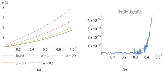
Figure 1. Profile of (a) exact and approximate solutions (b) absolute errors regarding $y_1$ for Example 4.

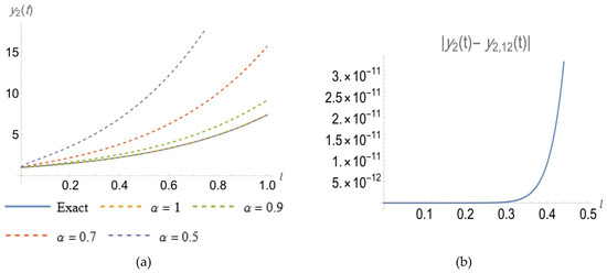
Figure 2. Profile of (a) exact and approximate solutions (b) absolute errors regarding $y_2$ for Example 4.

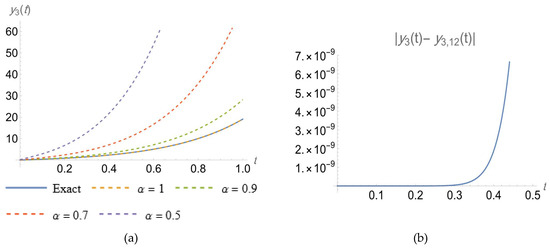
Figure 3. Profile of (a) exact and approximate solutions (b) absolute errors regarding $y_3$ for Example 4.

Example 5 [27]. 

Consider the following nonlinear system of fractional differential equations

$$\begin{array}{c}{D}^{\alpha }{y}_1\left(t\right)=-1002 y_1\left(t\right)+1000 y_2^2\left(t\right) \mathrm{and}\\ D^{\alpha }{y}_2\left(t\right)=y_1\left(t\right)-y_2\left(t\right)-y_2^2\left(t\right),\end{array}$$

(24)

with the ICs $y_1\left(0\right)=1$ and $y_2\left(0\right)=1, \mathrm{respectively}$.

The exact solutions to system (24) with $\alpha =1$ are $y_1\left(t\right)=e^{-2t} \mathrm{and} y_2\left(t\right)=e^{-t}.$

Solution. 

To solve system (24) using DPSM, apply the replacements from Theorem 3 on Equation (24), to obtain

$$\begin{array}{c}{D}^{\alpha }{y}_1\left(t\right)\leftrightarrow a_{n+1},\\ D^{\alpha }{y}_2\left(t\right)\leftrightarrow b_{n+1},\\ y_1\left(t\right)\leftrightarrow a_n,\\ y_2\left(t\right)\leftrightarrow b_n,\end{array}$$

and

$$y_2^2\left(t\right)\leftrightarrow {\displaystyle \sum }_{i=0}^n\frac{b_i{b}_{n-i}\mathsf{\Gamma }\left(n\alpha +1\right)}{\mathsf{\Gamma }\left(i\alpha +1\right)\mathsf{\Gamma }\left(\left(n-i\right)\alpha +1\right)},$$

where

$$\begin{array}{c}{a}_{n+1}=-1002a_n+1000{\displaystyle \sum }_{i=0}^n\frac{b_i{b}_{n-i}\mathsf{\Gamma }\left(n\alpha +1\right)}{\mathsf{\Gamma }\left(i\alpha +1\right)\mathsf{\Gamma }\left(\left(n-i\right)\alpha +1\right)} \mathrm{and}\\ b_{n+1}=a_n-b_n-{\displaystyle {\displaystyle \sum }_{i=0}^n}\frac{b_i{b}_{n-i}\mathsf{\Gamma }\left(n\alpha +1\right)}{\mathsf{\Gamma }\left(i\alpha +1\right)\mathsf{\Gamma }\left(\left(n-i\right)\alpha +1\right)}.\end{array}$$

(25)

Now, we have if:

$$\begin{array}{cc}n=0\to a_1& =-1002\left(1\right)+1000\left(1^2\right)=-2.\\ \hfill b_1& =1-1-\left(1^2\right)=-1.\hfill \\ n=1\to a_2& =-1002\left(-2\right)+1000\left(-2\right)=4.\\ \hfill b_2& =-2+1-\left(-2\right)=1,\hfill \\ n=2\to a_3& =-1002\left(4\right)+1000\left(\frac{\mathsf{\Gamma }\left(2\alpha +1\right)}{{\mathsf{\Gamma }}^2\left(\alpha +1\right)}+2\right)=-2008+1000\frac{\mathsf{\Gamma }\left(2\alpha +1\right)}{{\mathsf{\Gamma }}^2\left(\alpha +1\right)}.\\ \hfill b_3& =4-1-\left(\frac{\mathsf{\Gamma }\left(2\alpha +1\right)}{{\mathsf{\Gamma }}^2\left(\alpha +1\right)}+2\right)=1-\frac{\mathsf{\Gamma }\left(2\alpha +1\right)}{{\mathsf{\Gamma }}^2\left(\alpha +1\right)}.\hfill \\ n=3\to a_4& =-1002\left(-2008+1000\frac{\mathsf{\Gamma }\left(2\alpha +1\right)}{{\mathsf{\Gamma }}^2\left(\alpha +1\right)}\right)\\ & +1000\left(2-2\frac{\Gamma \left(2\alpha +1\right)}{{\Gamma }^2\left(\alpha +1\right)}-2\frac{\mathsf{\Gamma }\left(3\alpha +1\right)}{\mathsf{\Gamma }\left(\alpha +1\right)\mathsf{\Gamma }\left(2\alpha +1\right)}\right)\\ & =2014016-1004000\frac{\mathsf{\Gamma }\left(2\alpha +1\right)}{{\mathsf{\Gamma }}^2\left(\alpha +1\right)}-2000\frac{\mathsf{\Gamma }\left(3\alpha +1\right)}{\mathsf{\Gamma }\left(\alpha +1\right)\mathsf{\Gamma }\left(2\alpha +1\right)}.\\ \hfill b_4& =-2008+1000\frac{\mathsf{\Gamma }\left(2\alpha +1\right)}{{\mathsf{\Gamma }}^2\left(\alpha +1\right)}-1+\frac{\mathsf{\Gamma }\left(2\alpha +1\right)}{{\mathsf{\Gamma }}^2\left(\alpha +1\right)}-2+2\frac{\mathsf{\Gamma }\left(2\alpha +1\right)}{{\mathsf{\Gamma }}^2\left(\alpha +1\right)}\hfill \\ & +2\frac{\mathsf{\Gamma }\left(3\alpha +1\right)}{\mathsf{\Gamma }\left(\alpha +1\right)\mathsf{\Gamma }\left(2\alpha +1\right)}\\ & =-2011+1003\frac{\mathsf{\Gamma }\left(2\alpha +1\right)}{{\mathsf{\Gamma }}^2\left(\alpha +1\right)}+2\frac{\mathsf{\Gamma }\left(3\alpha +1\right)}{\mathsf{\Gamma }\left(\alpha +1\right)\mathsf{\Gamma }\left(2\alpha +1\right)}.\\ n=4\to a_5& =-1002\left(2014016-1004000\frac{\mathsf{\Gamma }\left(2\alpha +1\right)}{{\mathsf{\Gamma }}^2\left(\alpha +1\right)}-2000\frac{\mathsf{\Gamma }\left(3\alpha +1\right)}{\mathsf{\Gamma }\left(\alpha +1\right)\mathsf{\Gamma }\left(2\alpha +1\right)}\right)\\ & +1000(-4022+2006\frac{\mathsf{\Gamma }\left(2\alpha +1\right)}{{\mathsf{\Gamma }}^2\left(\alpha +1\right)}+\frac{\mathsf{\Gamma }\left(4\alpha +1\right)}{{\mathsf{\Gamma }}^2\left(2\alpha +1\right)}+4\frac{\mathsf{\Gamma }\left(3\alpha +1\right)}{\mathsf{\Gamma }\left(\alpha +1\right)\mathsf{\Gamma }\left(2\alpha +1\right)}\\ & -2\frac{\mathsf{\Gamma }\left(4\alpha +1\right)}{\mathsf{\Gamma }\left(\alpha +1\right)\mathsf{\Gamma }\left(3\alpha +1\right)}+2\frac{\mathsf{\Gamma }\left(2\alpha +1\right)\mathsf{\Gamma }\left(4\alpha +1\right)}{{\mathsf{\Gamma }}^3\left(\alpha +1\right)\mathsf{\Gamma }\left(3\alpha +1\right)})\\ & =-2022066032+1008014000\frac{\mathsf{\Gamma }\left(2\alpha +1\right)}{{\mathsf{\Gamma }}^2\left(\alpha +1\right)}+2008000\frac{\mathsf{\Gamma }\left(3\alpha +1\right)}{\mathsf{\Gamma }\left(\alpha +1\right)\mathsf{\Gamma }\left(2\alpha +1\right)}\\ & +1000\frac{\mathsf{\Gamma }\left(4\alpha +1\right)}{{\mathsf{\Gamma }}^2\left(2\alpha +1\right)}-2000\frac{\mathsf{\Gamma }\left(4\alpha +1\right)}{\mathsf{\Gamma }\left(\alpha +1\right)\mathsf{\Gamma }\left(3\alpha +1\right)}+2000\frac{\mathsf{\Gamma }\left(2\alpha +1\right)\mathsf{\Gamma }\left(4\alpha +1\right)}{{\mathsf{\Gamma }}^3\left(\alpha +1\right)\mathsf{\Gamma }\left(3\alpha +1\right)}.\\ \hfill b_5& =2014016-1004000\frac{\mathsf{\Gamma }\left(2\alpha +1\right)}{{\mathsf{\Gamma }}^2\left(\alpha +1\right)}-2000\frac{\mathsf{\Gamma }\left(3\alpha +1\right)}{\mathsf{\Gamma }\left(\alpha +1\right)\mathsf{\Gamma }\left(2\alpha +1\right)}\hfill \\ & -\left(-2011+1003\frac{\mathsf{\Gamma }\left(2\alpha +1\right)}{{\mathsf{\Gamma }}^2\left(\alpha +1\right)}+2\frac{\mathsf{\Gamma }\left(3\alpha +1\right)}{\mathsf{\Gamma }\left(\alpha +1\right)\mathsf{\Gamma }\left(2\alpha +1\right)}\right)\\ & -(-4022+2006\frac{\mathsf{\Gamma }\left(2\alpha +1\right)}{{\mathsf{\Gamma }}^2\left(\alpha +1\right)}+\frac{\mathsf{\Gamma }\left(4\alpha +1\right)}{{\mathsf{\Gamma }}^2\left(2\alpha +1\right)}+4\frac{\mathsf{\Gamma }\left(3\alpha +1\right)}{\mathsf{\Gamma }\left(\alpha +1\right)\mathsf{\Gamma }\left(2\alpha +1\right)}\\ & -2\frac{\mathsf{\Gamma }\left(4\alpha +1\right)}{\mathsf{\Gamma }\left(\alpha +1\right)\mathsf{\Gamma }\left(3\alpha +1\right)}+2\frac{\mathsf{\Gamma }\left(2\alpha +1\right)\mathsf{\Gamma }\left(4\alpha +1\right)}{{\mathsf{\Gamma }}^3\left(\alpha +1\right)\mathsf{\Gamma }\left(3\alpha +1\right)})\\ & =2020049-1007009\frac{\mathsf{\Gamma }\left(2\alpha +1\right)}{{\mathsf{\Gamma }}^2\left(\alpha +1\right)}-2006\frac{\mathsf{\Gamma }\left(3\alpha +1\right)}{\mathsf{\Gamma }\left(\alpha +1\right)\mathsf{\Gamma }\left(2\alpha +1\right)}\\ & -\frac{\mathsf{\Gamma }\left(4\alpha +1\right)}{{\mathsf{\Gamma }}^2\left(2\alpha +1\right)}+2\frac{\mathsf{\Gamma }\left(4\alpha +1\right)}{\mathsf{\Gamma }\left(\alpha +1\right)\mathsf{\Gamma }\left(3\alpha +1\right)}-2\frac{\mathsf{\Gamma }\left(2\alpha +1\right)\mathsf{\Gamma }\left(4\alpha +1\right)}{{\mathsf{\Gamma }}^3\left(\alpha +1\right)\mathsf{\Gamma }\left(3\alpha +1\right)}\end{array}$$

The approximate solutions to system (24) can be written as:

$$\begin{array}{cc}{y}_1& ={\displaystyle {\displaystyle \sum }_{n=0}^{\infty }}\frac{a_n{t}^{n\alpha }}{\mathsf{\Gamma }\left(n\alpha +1\right)}\\ & =1-\frac{2t^{\alpha }}{\mathsf{\Gamma }\left(\alpha +1\right)}+\frac{4t^{2\alpha }}{\mathsf{\Gamma }\left(2\alpha +1\right)}\\ & +\left(-2008+\frac{1000\mathsf{\Gamma }\left(2\alpha +1\right)}{{\mathsf{\Gamma }}^2\left(\alpha +1\right)}\right)\frac{t^{3\alpha }}{\mathsf{\Gamma }\left(3\alpha +1\right)}\\ & +(2014016-\frac{1004000\mathsf{\Gamma }\left(2\alpha +1\right)}{{\mathsf{\Gamma }}^2\left(\alpha +1\right)}\\ & -\frac{2000\mathsf{\Gamma }\left(3\alpha +1\right)}{\mathsf{\Gamma }\left(\alpha +1\right)\mathsf{\Gamma }\left(2\alpha +1\right)})\frac{t^{4\alpha }}{\mathsf{\Gamma }\left(4\alpha +1\right)}\\ & +(-2022066032+\frac{1008014000\mathsf{\Gamma }\left(2\alpha +1\right)}{{\mathsf{\Gamma }}^2\left(\alpha +1\right)}\\ & +\frac{2008000\mathsf{\Gamma }\left(3\alpha +1\right)}{\mathsf{\Gamma }\left(\alpha +1\right)\mathsf{\Gamma }\left(2\alpha +1\right)}+\frac{1000\mathsf{\Gamma }\left(4\alpha +1\right)}{{\mathsf{\Gamma }}^2\left(2\alpha +1\right)}\\ & -\frac{2000\mathsf{\Gamma }\left(4\alpha +1\right)}{\mathsf{\Gamma }\left(\alpha +1\right)\mathsf{\Gamma }\left(3\alpha +1\right)}\\ & +\frac{2000\mathsf{\Gamma }\left(2\alpha +1\right)\mathsf{\Gamma }\left(4\alpha +1\right)}{{\mathsf{\Gamma }}^3\left(\alpha +1\right)\mathsf{\Gamma }\left(3\alpha +1\right)})\frac{t^{5\alpha }}{\mathsf{\Gamma }\left(5\alpha +1\right)}+\cdots .\\ y_2& ={\displaystyle {\displaystyle \sum }_{n=0}^{\infty }}\frac{b_n{t}^{n\alpha }}{\mathsf{\Gamma }\left(n\alpha +1\right)}\\ & =1-\frac{t^{\alpha }}{\mathsf{\Gamma }\left(\alpha +1\right)}+\frac{t^{2\alpha }}{\mathsf{\Gamma }\left(2\alpha +1\right)}\\ & +\left(1-\frac{\mathsf{\Gamma }\left(2\alpha +1\right)}{{\mathsf{\Gamma }}^2\left(\alpha +1\right)}\right)\frac{t^{3\alpha }}{\mathsf{\Gamma }\left(3\alpha +1\right)}\\ & +(-2011+\frac{1003\mathsf{\Gamma }\left(2\alpha +1\right)}{{\mathsf{\Gamma }}^2\left(\alpha +1\right)}\\ & +\frac{2\mathsf{\Gamma }\left(3\alpha +1\right)}{\mathsf{\Gamma }\left(\alpha +1\right)\mathsf{\Gamma }\left(2\alpha +1\right)})\frac{t^{4\alpha }}{\mathsf{\Gamma }\left(4\alpha +1\right)}\\ & +(2020049-\frac{1007009\mathsf{\Gamma }\left(2\alpha +1\right)}{{\mathsf{\Gamma }}^2\left(\alpha +1\right)}\\ & -\frac{2006\mathsf{\Gamma }\left(3\alpha +1\right)}{\mathsf{\Gamma }\left(\alpha +1\right)\mathsf{\Gamma }\left(2\alpha +1\right)}-\frac{\mathsf{\Gamma }\left(4\alpha +1\right)}{{\mathsf{\Gamma }}^2\left(2\alpha +1\right)}\\ & +\frac{2\mathsf{\Gamma }\left(4\alpha +1\right)}{\mathsf{\Gamma }\left(\alpha +1\right)\mathsf{\Gamma }\left(3\alpha +1\right)}\\ & -\frac{2\mathsf{\Gamma }\left(2\alpha +1\right)\mathsf{\Gamma }\left(4\alpha +1\right)}{{\mathsf{\Gamma }}^3\left(\alpha +1\right)\mathsf{\Gamma }\left(3\alpha +1\right)})\frac{t^{5\alpha }}{\mathsf{\Gamma }\left(5\alpha +1\right)}+\cdots .\end{array}$$

This problem is introduced in [26] and the authors computed the second approximation only, but using DPSM, the steps are shown completely until the fifth approximation, which is more accurate. The solutions calculated by the Mathematica program were computed to the twelfth approximation, and the errors are considered in the below tables.

Moreover, we note that the numerical results are identical to that obtained by the Laplace residual power series method [12]. The CPU time spent to complete Table 4 below was $0.0004346$ s, and to complete Table 5, it was $0.005228$ s.

Table 4. Error analysis of $y_1\left(t\right)$ for Example 5 on $\left[0,1\right]$.

	Exact Solution	Solution by DPSM	$\left|{\mathit{y}}_1\left(\mathit{t}\right)-{\mathit{y}}_{1,12}\left(\mathit{t}\right)\right|$
$0.16$	$0.726149$	$0.726149$	$0$
$0.32$	$0.527292$	$0.527292$	$4.63962\times {10}^{-13}$
$0.48$	$0.382893$	$0.382893$	$8.83733\times {10}^{-11}$
$0.64$	$0.278037$	$0.278037$	$3.64122\times {10}^{-9}$
$0.8$	$0.201897$	$0.201897$	$6.48591\times {10}^{-8}$
$0.96$	$0.146607$	$0.146607$	$6.79809\times {10}^{-7}$

Table 5. Error analysis of $y_2\left(t\right)$ for Example 5 on $\left[0,1\right]$.

	Exact Solution	Solution by DPSM	$\left|{\mathit{y}}_2\left(\mathit{t}\right)-{\mathit{y}}_{2,12}\left(\mathit{t}\right)\right|$
$0.16$	$0.852114$	$0.852114$	$2.22045\times {10}^{-16}$
$0.32$	$0.726149$	$0.726149$	$0$
$0.48$	$0.618783$	$0.618783$	$1.13243\times {10}^{-14}$
$0.64$	$0.527292$	$0.527292$	$4.63962\times {10}^{-13}$
$0.8$	$0.449329$	$0.449329$	$\mathrm{8.8.34971}\times {10}^{-12}$
$0.96$	$0.382893$	$0.382893$	$8.83733\times {10}^{-11}$

The following figures illustrate the exact solutions, approximate solutions, and the exact errors of $y_1$ and $y_2$. The CPU time that is spent to complete Figure 4 and Figure 5, respectively, are $\left(0.1274689\right) \mathrm{and} \left(0.049291\right) \mathrm{s} \mathrm{and} \left(0.1531077\right) \mathrm{and} \left(0.17544980\right)$ s.

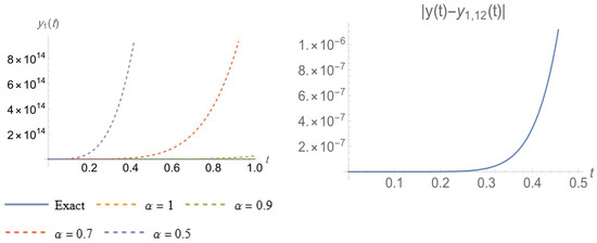
Figure 4. Profile of exact and approximate solutions and absolute errors regarding $y_1$ for Example 5.

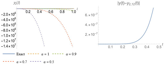
Figure 5. Profile of exact and approximate solutions and absolute errors regarding $y_2$ for Example 5.

Example 6 [27]. 

Consider the three-dimensional pantograph equations

$$\begin{array}{c}{y}_1^{\prime }\left(t\right)=2y_2\left(\frac{t}{2}\right)+y_3\left(t\right)-t\cos \left(\frac{t}{2}\right) ,\\ y_2^{\prime }\left(t\right)=1-t\sin t-2y_3^2\left(\frac{t}{2}\right), \mathrm{and}\\ y_3^{\prime }=y_2\left(t\right)-y_1\left(t\right)-t\cos t \end{array}$$

(26)

with the ICs $y_1\left(0\right)=-1, y_2\left(0\right)=0, \mathrm{and} y_3\left(0\right)=0, \mathrm{respectively}$.

Solution. 

To solve system (26) by DPSM, first let us write Tayler series of the functions

$$\begin{array}{cc}f\left(t\right)& =-t\cos \frac{t}{2} \Rightarrow f\left(t\right)=-t+\frac{3}{4}{\frac{t}{3!}}^3-\frac{5}{16}{\frac{t}{5!}}^5+\dots ,\\ g\left(t\right)& =1-t\sin t\Rightarrow g\left(t\right)\\ & =1-2{\frac{t}{2}}^2+4{\frac{t}{4}}^4-6{\frac{t}{6}}^6+\cdots , \mathrm{and}\\ h\left(t\right)& =-t\cos \mathrm{t}\Rightarrow h\left(t\right)=-t+\frac{3t^3}{3!}-\frac{5t^5}{5!}+\cdots .\end{array}$$

Then,

$$\begin{array}{c}{f}_0=f_2=f_4=f_6=f_8=0,\\ f_1=-1, f_3=\frac{3}{4}, f_5=\frac{-5}{16}, f_7=\frac{7}{64}, f_9=\frac{-9}{256},\\ g_0=1, g_2=-2, g_4=4, g_6=-6, g_8=8 ,\\ g_1=g_3=g_5=g_7=g_9=0,\end{array}$$

and

$$\begin{array}{c}{h}_0=h_2=h_4=h_6=h_8=0,\\ h_1=-1, h_3=3, h_5=-5, h_7=7, h_9=-9.\end{array}$$

Using DPSM, the solution is obtained after applying the replacements in Theorem 3, as follows:

$$\begin{array}{c}{y}_1^{\prime }\left(t\right)\leftrightarrow a_{n+1},\\ y_2^{\prime }\left(t\right)\leftrightarrow b_{n+1},\\ y_3^{\prime }\left(t\right)\leftrightarrow c_{n+1},\\ y_1\left(t\right)\leftrightarrow a_n,\\ y_2\left(t\right)\leftrightarrow b_n,\\ y_3\left(t\right)\leftrightarrow c_n,\\ y_2\left(\frac{t}{2}\right)\leftrightarrow {\left(\frac{1}{2}\right)}^n{b}_n,\end{array}$$

and

$$y_3^2\left(\frac{t}{2}\right)\leftrightarrow {\left(\frac{1}{2}\right)}^n{\displaystyle \sum }_{i=0}^n\frac{c_i{c}_{n-i}n!}{i!\left(n-i\right)!}.$$

where,

$$\begin{array}{c}{a}_{n+1}=2{\left(\frac{1}{2}\right)}^n{b}_n+c_n+f_n.\\ b_{n+1}=g_n-2{\left(\frac{1}{2}\right)}^n{\displaystyle {\displaystyle \sum }_{i=0}^n}\frac{c_i{c}_{n-i}n!}{i!\left(n-i\right)!}.\\ c_{n+1}=b_n-a_n+h_n.\end{array}$$

(27)

Now,

For $n=0,$ $a_1=0+0+0=0.$ $b_1=1-0=1.$ $c_1=0-\left(-1\right)+0=1.$	For $n=1,$ $a_2=2{\left(\frac{1}{2}\right)}^{1}1+1-1=1.$ $b_2=0-0=0.$ $c_2=1-0-1=0.$
For $n=2,$ $a_3=0+0+0=0.$ $b_3=-2-2{\left(\frac{1}{2}\right)}^2\left(\frac{1\left(2!\right)}{1!1!}\right)=-3.$ $c_3=0-1+0=-1.$	For $n=3,$ $a_4=2{\left(\frac{1}{2}\right)}^3\left(-3\right)+\left(-1\right)+\frac{3}{4}=-1.$ $b_4=0-0=0.$ $c_4=-3-0+3=0.$
For $n=4,$ $a_5=0+0+0=0.$ $b_5=4-2{\left(\frac{1}{2}\right)}^4\left(\frac{2\left(-1\right)\left(4!\right)}{1!3!}\right)=5.$ $c_5=0-\left(-1\right)+0=1.$	For $n=5,$ $a_6=2{\left(\frac{1}{2}\right)}^5\left(5\right)+1-\frac{5}{16}=1.$ $b_6=0-0=0.$ $c_6=5-0-5=0.$
For $n=6,$ $a_7=0+0+0=0.$ $b_7=-6-2{\left(\frac{1}{2}\right)}^6\left(\frac{\left(2\right)\left(1\right)}{1!5!}+\frac{{\left(-1\right)}^2}{3!3!}\right)6!=-7.$ $c_7=0-1+0=-1.$	For $n=7,$ $a_8={\left(\frac{1}{2}\right)}^6\left(-7\right)+-1+\frac{7}{64}=-1.$ $b_8=0-{\left(\frac{1}{2}\right)}^6\left(0\right)=0.$ $c_8=-7-0+7=0.$
For $n=8,$ $a_9={\left(\frac{1}{2}\right)}^7\left(0\right)+0+0=0.$ $b_9=8-{\left(\frac{1}{2}\right)}^7\left(\frac{2\left(1\right)\left(-1\right)8!}{1!7!}+\frac{2\left(1\right)\left(-1\right)8!}{3!5!}\right)=9.$ $c_9=0-\left(-1\right)+0=1.$	For $n=9,$ $a_{10}={\left(\frac{1}{2}\right)}^8\left(9\right)+1-\frac{9}{256}=1.$ $b_{10}=0-{\left(\frac{1}{2}\right)}^8\left(0\right)=0.$ $c_{10}=9-0-9=0$.

Then,

$$\begin{array}{c}{y}_{1,10}\left(t\right)={\displaystyle {\displaystyle \sum }_{n=0}^{10}}\frac{a_n{t}^n}{n!}=-1+\frac{t^2}{2!}-\frac{t^4}{4!}+\frac{t^6}{6!}-\frac{t^8}{8!}+\frac{t^{10}}{10!}.\\ y_{2,10}\left(t\right)={\displaystyle {\displaystyle \sum }_{n=0}^{10}}\frac{b_n{t}^n}{n!}=t-3\frac{t^3}{3!}+5\frac{t^5}{5!}-7\frac{t^7}{7!}+9\frac{t^9}{9!}.\\ y_{3,10}\left(t\right)={\displaystyle {\displaystyle \sum }_{n=0}^{10}}\frac{c_n{t}^n}{n!}=t-\frac{t^3}{3!}+\frac{t^5}{5!}-\frac{t^7}{7!}+\frac{t^9}{9!}.\end{array}$$

(28)

In the following tables, Table 6, Table 7 and Table 8, we present the tenth approximate solutions of $y_1,y_2$ and $y_3$ respectively by the DPSM.

Table 6. Error analysis of $y_1\left(t\right)$ for Example 6 on $\left[0,1\right]$.

	Exact Solution	Solution by DPSM	$\left|{\mathit{y}}_1\left(\mathit{t}\right)-{\mathit{y}}_{1,10}\left(\mathit{t}\right)\right|$	$\left|\frac{{\mathit{y}}_1\left(\mathit{t}\right)-{\mathit{y}}_{1,10}\left(\mathit{t}\right)}{{\mathit{y}}_1\left(\mathit{t}\right)}\right|$
$0.2$	$-0.980067$	$-0.980067$	$0$	$0$
$0.4$	$-0.921061$	$-0.921061$	$3.5083\times {10}^{-14}$	$3.80898\times {10}^{-14}$
$0.6$	$-0.825336$	$-0.825336$	$4.53548\times {10}^{-12}$	$5.49532\times {10}^{-12}$
$0.8$	$-0.696707$	$-0.696707$	$1.42961\times {10}^{-10}$	$2.05195\times {10}^{-10}$
$1$	$-0.540302$	$-0.540302$	$2.07625\times {10}^{-9}$	$3.84276\times {10}^{-9}$

Table 7. Error analysis of $y_2\left(t\right)$ for Example 6 on $\left[0,1\right]$.

	Exact Solution	Solution by DPSM	$\left|{\mathit{y}}_2\left(\mathit{t}\right)-{\mathit{y}}_{2,10}\left(\mathit{t}\right)\right|$	$\left|\frac{{\mathit{y}}_2\left(\mathit{t}\right)-{\mathit{y}}_{2,10}\left(\mathit{t}\right)}{{\mathit{y}}_2\left(\mathit{t}\right)}\right|$
$0.2$	$0.196013$	$0.196013$	$5.66214\times {10}^{-15}$	$2.88865\times {10}^{-14}$
$0.4$	$0.368424$	$0.368424$	$1.15443\times {10}^{-11}$	$3.13343\times {10}^{-11}$
$0.6$	$0.495201$	$0.495201$	$9.9705\times {10}^{-10}$	$2.01342\times {10}^{-9}$
$0.8$	$0.557365$	$0.557365$	$2.35572\times {10}^{-8}$	$4.22653\times {10}^{-8}$
$1$	$0.540302$	$0.540302$	$2.73497\times {10}^{-7}$	$5.06192\times {10}^{-7}$

Table 8. Error analysis of $y_3\left(t\right)$ for Example 6 on $\left[0,1\right]$.

	Exact Solution	Solution by DPSM	$\left|{\mathit{y}}_3\left(\mathit{t}\right)-{\mathit{y}}_{3,10}\left(\mathit{t}\right)\right|$	$\left|\frac{{\mathit{y}}_3\left(\mathit{t}\right)-{\mathit{y}}_{3,10}\left(\mathit{t}\right)}{{\mathit{y}}_3\left(\mathit{t}\right)}\right|$
$0.2$	$0.198669$	$0.198669$	$5.55112\times {10}^{-16}$	$2.79415\times {10}^{-15}$
$0.4$	$0.389418$	$0.389418$	$1.04966\times {10}^{-12}$	$2.69546\times {10}^{-12}$
$0.6$	$0.564642$	$0.564642$	$9.06788\times {10}^{-11}$	$1.60595\times {10}^{-10}$
$0.8$	$0.717356$	$0.717356$	$2.14316\times {10}^{-9}$	$2.98758\times {10}^{-9}$
$1$	$0.841471$	$0.841471$	$2.48923\times {10}^{-8}$	$2.95819\times {10}^{-8}$

In addition, the errors and relative errors are illustrated in the tables up to the tenth approximations. The CPU time spent to complete Table 6 was $0.0330754$ s, and to complete Table 7, it was $0.0001189$ s, and for Table 8, it was $0.0001083 \mathrm{s}.$

The following figures (Figure 6, Figure 7 and Figure 8) show graphs of the approximate solutions using DPSM, with different values of $k$ (approximate levels), for $y_1, y_{2,}$ and $y_3,$ respectively. The CPU time spent to complete Figure 6, Figure 7 and Figure 8, respectively, was 0.0351227, $0.0348473, \mathrm{and} 0.0352323$ s.

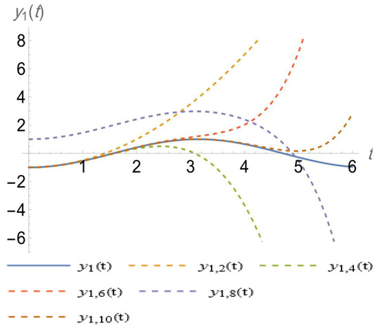
Figure 6. Plots of the exact solution for $y_1\left(t\right)$ and the solution using DPSM for $y\left(t\right)$, with $k=2,4,6,8,10$ for Example 6 on [0,6], where $y_1\left(t\right)$ and $y_{1,k}\left(t\right)$ are represented, respectively, by straight and dashed lines.

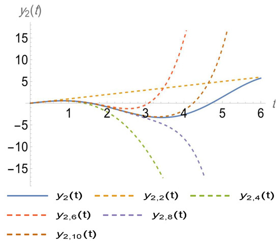
Figure 7. Plots of the exact solution for $y_2\left(t\right)$ and the solution using DPSM for $y_{2,k}\left(t\right)$, with $k=2,4,6,8,10$ for Example 6 on [0,6], where $y_2\left(t\right)$ and $y_{2,k}\left(t\right)$ are represented, respectively, by straight and dashed lines.

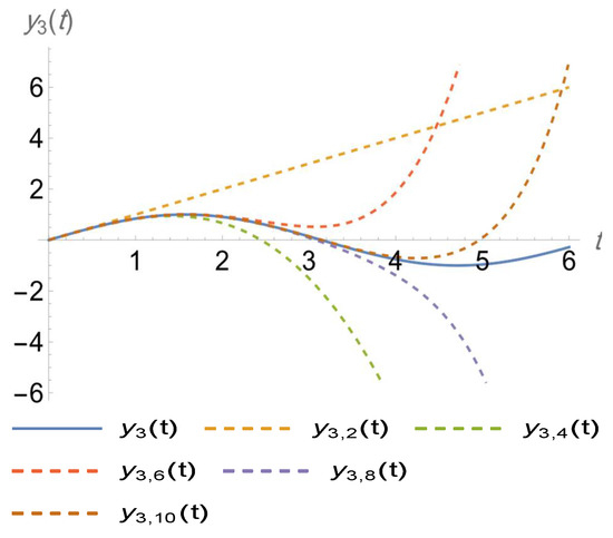
Figure 8. Plots of the exact solution for $y_3\left(t\right)$ and the solution using DPSM for $y_{3,k}\left(t\right)$, with $k=2,4,6,8,10$ for Example 6 on [0,6], where $y_3\left(t\right)$ and $y_{3,k}\left(t\right)$ are represented, respectively, by straight and dashed lines.

5. Remarks and Discussion

In this section, we introduce remarks and discussion about the presented method.

• The new technique, DPSM, depends on obtaining numerical series solutions to differential equations using the idea of the power series method.
• The method is applicable and efficient in finding approximate solutions to differential equations of different types.
• There is no need to compute limits or derivatives through the applications.
• The method can be easily programmed by computer software.
• DPSM saves time and effort for researchers in obtaining analytical solutions.
• DPSM requires no linearization or discretization to apply, which is different from other analytical methods.
• We can obtain many terms of the approximate solution using the general term that we obtain using DPSM for the target equation.
• Unlike other analytical methods, DPSM can guarantee finding a general term of the series solution.
• All the numerical results in this article were obtained using the Mathematica 13 software.
• DPSM provides the same results as those obtained by other power series methods, which guarantees its reliability, but it is faster and simpler than other methods.

6. Conclusions

In different types of sciences, such as mathematics, physics, engineering statics, etc., there are large numbers of equations and systems that need to be solved. Mathematicians have created and developed many analytical and numerical methods to obtain the right answer exactly or approximately. Power series methods, such as RPSM, the Laplace residual power series method, and many others, provide precise solutions, and sometimes, they provide the exact solution. However, these methods require many steps each time, especially when solving nonlinear equations and systems. This article introduces a new method, called DPSM, that presents series solutions to some types of problems directly and without long computations. This method is simple compared to other methods and it provides more accurate results than other power series methods because it can generate many terms of the series solution that could be easily programmed to be found more quickly by computer software (Mathematica). DPSM is a simple method that calculates the coefficients of the power series expansion directly, without hard calculations. The obtained results demonstrate the applicability and efficiency of the proposed method. In the future, we will pay attention to obtaining new formulas to solve linear and nonlinear PDEs of fractional orders.

References

- Almeida, R.; Torres, D.F. Necessary and sufficient conditions for the fractional calculus of variations with Caputo derivatives. Commun. Nonlinear Sci. Numer. Simul. 2011, 16, 1490–1500. [Google Scholar] [CrossRef]
- Podlubny, I. Fractional Differential Equations; Elsevier: Amsterdam, The Netherlands, 1999. [Google Scholar]
- Mainardi, F. Fractional Calculus and Waves in Linear Viscoelasticity; Imperial College Press: London, UK, 2010. [Google Scholar]
- Kumar, S.; Kumar, R.; Osman, M.S.; Samet, B.A. Wavelet based numerical scheme for fractional order SEIR epidemic of measles by using Genocchi polynomials. Numer. Methods Partial. Differ. Equ. 2021, 37, 1250–1268. [Google Scholar] [CrossRef]
- Matlob, M.A.; Jamali, Y. The concepts and applications of fractional order differential calculus in modeling of viscoelastic systems: A primer. Crit. Rev. Biomed. Eng. 2019, 47, 249–276. [Google Scholar] [CrossRef] [PubMed]
- Kumar, P.; Qureshi, S. Laplace-Carson integral transform for exact solutions of non-integer order initial value problems with Caputo operator. J. Appl. Math. Comput. Mech. 2020, 19, 57–66. [Google Scholar] [CrossRef]
- D’Elia, M.; Du, Q.; Glusa, C.; Gunzburger, M.; Tian, X.; Zhou, Z. Numerical methods for nonlocal and fractional models. Acta Numer. 2020, 29, 1–124. [Google Scholar] [CrossRef]
- Kilbas, A.; Srivasfava, H.; Trujillo, J. Theory and Applications of Fractional Differential Equation. In North-Holland Mathematics Studies; Elsevier Science BV: Amsterdam, The Netherlands, 2006. [Google Scholar]
- Baleanu, D.; Diethelm, K.; Scalas, E.; Trujillo, J.J. Fractional Calculus: Models and Numerical Methods; World Scientific: Singapore, 2012; Volume 3. [Google Scholar]
- Zhang, Y.; Kumar, A.; Kumar, S.; Baleanu, D.; Yang, X.J. Residual power series method for time-fractional Schrödinger equations. J. Nonlinear Sci. Appl. 2016, 9, 5821–5829. [Google Scholar] [CrossRef]
- Burqan, A.; Saadeh, R.; Qazza, A. ARA-Residual Power Series Method for Solving Partial Fractional Differential Equations. Alex. Eng. J. 2022, 62, 47–62. [Google Scholar] [CrossRef]
- Qazza, A.; Burqan, A.; Saadeh, R. Application of ARA Residual Power Series Method in Solving Systems of Fractional Differential Equations. Math. Probl. Eng. 2022, 2022, 6939045. [Google Scholar] [CrossRef]
- Kumar, S.; Kumar, A.; Baleanu, D. Two analytical methods for time-fractional nonlinear coupled Boussinesq–Burger’s equations arise in propagation of shallow water waves. Nonlinear Dyn. 2016, 85, 699–715. [Google Scholar] [CrossRef]
- Kumar, A.; Kumar, S.; Singh, M. Residual power series method for fractional Sharma-Tasso-Olever equation. Commun. Numer. Anal. 2016, 10, 1–10. [Google Scholar] [CrossRef]
- El-Ajou, A.; Arqub, O.A.; Zhour, Z.A.; Momani, S. New results on fractional power series: Theories and applications. Entropy 2013, 15, 5305–5323. [Google Scholar] [CrossRef]
- Shokooh, A.; Suárez, L. A comparison of numerical methods applied to a fractional model of damping materials. J. Vib. Control 1999, 5, 331–354. [Google Scholar] [CrossRef]
- Alquran, M.; Ali, M.; Alsukhour, M.; Jaradat, I. Promoted residual power series technique with Laplace transform to solve some time-fractional problems arising in physics. Results Phys. 2020, 19, 103667. [Google Scholar] [CrossRef]
- Wu, G.C.; Baleanu, D. Variational iteration method for fractional calculus—A universal approach by Laplace transform. Adv. Differ. Equ. 2013, 1, 18. [Google Scholar] [CrossRef]
- Thongmoon, M.; Pusjuso, S. The numerical solutions of differential transform method and the Laplace transform method for a system of differential equations. Nonlinear Anal. Hybrid Syst. 2010, 4, 425–431. [Google Scholar] [CrossRef]
- Diethelm, K.; Ford, N.J.; Freed, A.D.; Luchko, Y. Algorithms for the fractional calculus: A selection of numerical methods. Comput. Methods Appl. Mech. Eng. 2005, 194, 743–773. [Google Scholar] [CrossRef]
- Ezz-Eldien, S.S. On solving systems of multi-pantograph equations via spectral tau method. Appl. Math. Comput. 2018, 321, 63–73. [Google Scholar] [CrossRef]
- Abu-Gdairi, R. Analytical Solution of Nonlinear Fractional Gradient-Based System Using Fractional Power Series Method. Int. J. Anal. Appl. 2022, 20, 51. [Google Scholar] [CrossRef]
- Ahmed, S.A.; Qazza, A.; Saadeh, R. Exact Solutions of Nonlinear Partial Differential Equations via the New Double Integral Transform Combined with Iterative Method. Axioms 2022, 11, 247. [Google Scholar] [CrossRef]
- Eriqat, T.; El-Ajou, A.; Moa’ath, N.O.; Al-Zhour, Z.; Momani, S. A new attractive analytic approach for solutions of linear and nonlinear neutral fractional pantograph equations. Chaos Solitons Fractals 2020, 138, 109957. [Google Scholar] [CrossRef]
- Alquran, M.; Alsukhour, M.; Ali, M.; Jaradat, I. Combination of Laplace transform and residual power series techniques to solve autonomous n-dimensional fractional nonlinear systems. Nonlinear Eng. 2021, 10, 282–292. [Google Scholar] [CrossRef]
- Rani, A.; Saeed, M.; Ul-Hassan, Q.M.; Ashraf, M.; Khan, M.Y.; Ayub, K. Solving system of differential equations of fractional order by homotopy analysis method. J. Sci. Arts 2017, 17, 457–468. [Google Scholar]
- Komashynska, I.; Al-Smadi, M.; Al-Habahbeh, A.; Ateiwi, A. Analytical Approximate Solutions of Systems of Multi-pantograph Delay Differential Equations Using Residual Power-series Method. Aust. J. Basic Appl. Sci. 2014, 8, 664–675. [Google Scholar]
- Nieto, J.J. Solution of a fractional logistic ordinary differential equation. Appl. Math. Lett. 2022, 123, 107568. [Google Scholar] [CrossRef]
- Hattaf, K. On the stability and numerical scheme of fractional differential equations with application to biology. Computation 2022, 10, 97. [Google Scholar] [CrossRef]
- Agarwal, R.P.; Benchohra, M.; Hamani, S. Boundary value problems for fractional differential equations. Georgian Math. J. 2009, 16, 401–411. [Google Scholar] [CrossRef]
- Weilbeer, M. Efficient Numerical Methods for Fractional Differential Equations and Their Analytical Background. Ph.D. Thesis, Technical University of Braunschweig, Braunschweig, Germany, 2006. [Google Scholar]
- Ismail, G.; Abdl-Rahim, H.; Ahmad, H.; Chu, Y. Fractional residual power series method for the analytical and approximate studies of fractional physical phenomena. Open Phys. 2020, 18, 799–805. [Google Scholar] [CrossRef]
- Chen, S.B.; Soradi-Zeid, S.; Alipour, M.; Chu, Y.M.; Gomez-Aguilar, J.F.; Jahanshahi, H. Optimal control of nonlinear time-delay fractional differential equations with Dickson polynomials. Fractals 2021, 29, 2150079. [Google Scholar] [CrossRef]
- Chu, Y.M.; Hani, E.H.B.; El-Zahar, E.R.; Ebaid, A.; Shah, N.A. Combination of Shehu decomposition and variational iteration transform methods for solving fractional third order dispersive partial differential equations. Numer. Methods Partial Differ. Equ. 2021. [Google Scholar] [CrossRef]
Disclaimer/Publisher’s Note: The statements, opinions and data contained in all publications are solely those of the individual author(s) and contributor(s) and not of MDPI and/or the editor(s). MDPI and/or the editor(s) disclaim responsibility for any injury to people or property resulting from any ideas, methods, instructions or products referred to in the content. |
© 2023 by the authors. Licensee MDPI, Basel, Switzerland. This article is an open access article distributed under the terms and conditions of the Creative Commons Attribution (CC BY) license (https://creativecommons.org/licenses/by/4.0/).