Dynamics Analysis of a Discrete-Time Commensalism Model with Additive Allee for the Host Species

Abstract

We propose and study a class of discrete-time commensalism systems with additive Allee effects on the host species. First, the single species with additive Allee effects is analyzed for existence and stability, then the existence of fixed points of discrete systems is given, and the local stability of fixed points is given by characteristic root analysis. Second, we used the center manifold theorem and bifurcation theory to study the bifurcation of a codimension of one of the system at non-hyperbolic fixed points, including flip, transcritical, pitchfork, and fold bifurcations. Furthermore, this paper used the hybrid chaos method to control the chaos that occurs in the flip bifurcation of the system. Finally, the analysis conclusions were verified by numerical simulations. Compared with the continuous system, the similarities are that both species’ densities decrease with increasing Allee values under the weak Allee effect and that the host species hastens extinction under the strong Allee effect. Further, when the birth rate of the benefited species is low and the time is large enough, the benefited species will be locally asymptotically stabilized. Thus, our new finding is that both strong and weak Allee effects contribute to the stability of the benefited species under certain conditions.

1. Introduction

Interactions between different species play a crucial role in shaping and maintaining balance within ecosystems. Interspecies interactions hold the potential to deliver mutual advantages, inflict harm, or yield no discernible impact on each of the participating species. These interactions are categorized by paired outcomes, symbolized as a positive, negative, or neutral result [1]. Commensal relationships, where one species gains a benefit while the other is unaffected, are often cited in the ecological literature, yet they receive surprisingly limited attention in research. In ecosystems, both commensalism and mutualism models involve positive interactions between populations. There is no harm in commensalism, in which one side is beneficial, while the other side is not beneficial and harmless.

A Belgian zoologist named Pierre-Joseph van Beneden was the pioneer in situating commensalism within a biological context. He contrasted commensalism with two other types of interactions: parasitism and mutualism [1]. In mutualism, species are interdependent and both benefit, while in commensalism, one species gains advantages without strong dependency or notable harm to the other. Despite its milder impact, commensalism adds complexity to ecological relationships and community organization. According to [2,3], depending on the population density, in some cases, the mutualism relationship shifts to a resemblance closer to commensalism, e.g., the relation among the carnivorous plant Roridula dentata and hemipteran Pameridae marlothii. The larvae of midges and mosquitoes that live on pitcher plants exhibit a commensalism relationship. Midges, as upstream resource consumers, produce large quantities of bacteria and particles that contribute to the growth of mosquitoes. However, the experiments in [4] showed that mosquitoes do not affect midges. There is a symbiotic relationship between the two. Hari Prasad [5] pointed out that small green epiphytes that grow on other plants prepare themselves for survival by occupying the space of other plants to absorb the water and minerals that the roots obtain from the air. In turn, plants are unaffected. Squirrels burrow intooak trees for living space and food storage. Yet, the oak is neither beneficial nor harmful. To avoid it enemies, the clownfish will choose to hide in the tentacles of the sea anemone, and the tentacles are not affected by the clownfish, and so on.

From the standpoint of mathematical modeling, the investigation of the commensalism system was pioneered by Sun and Wei [6] in 2003. They were the first to explore this area using a two-species model. Over the past few years, an increasing number of researchers have directed their focus towards utilizing mathematical modeling methods to explore the commensalism model among populations (see [7,8,9,10,11,12,13,14,15,16,17] and the references therein). Afterwards, Han et al. [18] proposed a continuous time Lotka–Volterra-type commensalism system as follows:

$$\left\{\begin{array}{c}{\displaystyle \frac{\mathrm{d}x}{\mathrm{d}t}={\displaystyle x\left(b_1-a_{11}x\right)+a_{12}xy,}}\hfill \\ {\displaystyle }\hfill \\ {\displaystyle \frac{\mathrm{d}y}{\mathrm{d}t}=y\left(b_2-a_{22}y\right),}\hfill \end{array}\right.$$

(1)

where $x\left(0\right)>0,y\left(0\right)>0$ and $t\in [0,\infty )$. $x\left(t\right)$ and $y\left(t\right)$ denote the population densities of the commensal and host, respectively, at time t; $b_1$ and $b_2$ denote the intrinsic growth rates of the two species, respectively; $a_{11}$ and $a_{22}$ denote the intraspecific competition coefficient of the commensal and host; $a_{12}>0$ denotes the coefficient of influence that the host produces in the commensal. We should notice that $b_1,a_{11},a_{12},b_2,a_{22}$ are positive constants. The authors’ study showed that Model (1) has a globally stable coexistence fixed point. Next, feedback control is considered by adding control variables. The results showed that the position of the coexistence fixed point is altered without affecting its global steady-state properties.

After that, many scholars began to consider the effects of various factors based on the system (1) and analyze the dynamic behaviors of the corresponding systems, for example periodic solutions [19,20], harvesting [21,22,23,24,25], the Allee effect [26,27,28], and delay [29,30]. In [19], the authors investigated a modified commensal symbiosis model with Michaelis–Menten-type harvesting and observed positive periodic solutions. In [20], Chen et al. presented another discrete commensal symbiosis model with a Hassell–Varley-type functional response. Their study revealed a positive periodic solution of the system, which is both locally and globally stable. Considering a Lotka–Volterra-type commensal model subject to the Allee effect on the unaffected species, which occurs at a low population density, Xinyu Guan [27] observed that the Allee effect has no influence on the final densities of the unaffected species and the benefited species. The study involved numerical simulations that demonstrated a considerable elongation in the time required for the system subjected to an Allee effect to attain its stable steady-state solution, implying that the Allee effect has an unstable effect on the system. In [28], the authors explored a discrete-time commensal symbiosis model and observed period-doubling bifurcation phenomenon around the interior equilibrium state.

According to previous studies by W.C. Allee, population density has a positive impact on reproduction in a wide range of terrestrial and aquatic species. It could potentially contribute to the prolonged survival of the species in unfavorable environments and provide increased protection against harmful substances [31,32]. When the population density drops below a specific threshold or when the population is too diminutive, the task of finding a mate can become more challenging. Similarly, in species where group activities such as fending off predators or searching for sustenance are impeded due to low population densities, these activities become less proficient. This positive correlation between population size and individual fitness is termed the Allee effect. In the past few years, populations from various ecosystems have become low or even at risk of becoming endangered due to escalating human predation, heightened occurrences of natural disasters, and rising global temperatures. In such situations, the populations may have trouble mating, foraging, and fending off natural enemies. Previous mathematical studies have shown that Allees add more complexity to the system’s dynamic behavior [33,34]. In 2022, He et al. [11] proposed the following continuous-time commensalism system incorporating an additive Allee to the host:

$$\left\{\begin{array}{c}{\displaystyle \frac{\mathrm{d}x}{\mathrm{d}t}=x\left(r-bx\right)+cxy,}\hfill \\ {\displaystyle }\hfill \\ {\displaystyle \frac{\mathrm{d}y}{\mathrm{d}t}=y\left(d-ey-\frac{m}{y+a}\right),}\hfill \end{array}\right.$$

(2)

where all of the parameters are positive constants and initial values are $x\left(0\right)>0,y\left(0\right)>0$, and $t\in [0,\infty )$, the same as the previous definition in [11]. He et al. [11] gave the existence and local stability of equilibrium points, then proved that, under suitable conditions, $E_r(\frac{r}{b},0)$ and $E_1^{*}(x_1^{*},y_1)$ are globally asymptotically stable, respectively. There are saddle-node bifurcation at $E_3^{*}(x_3^{*},y_3)$, $E_3(0,y_3)$ and transcritical bifurcation at $E_0(0,0)$, $E_r(\frac{r}{b},0)$, respectively.

In recent years, discrete-time systems have also been one of the hotspots of scholars’ research. The reason is that populations with non-overlapping generations are better described by difference equations, which are also easier to simulate numerically. Discrete-time systems also have more topological classifications and bifurcations at fixed points than corresponding continuous-time systems, with a codimension of one, such as flip, transcritical, pitchfork, fold, and Neimark–Sacker bifurcations, and a codimension of two, such as 1:1 and 1:2, and fold–flip bifurcations, e.g., [35,36,37,38,39,40,41]. To the best of the authors’ knowledge, limited research has been conducted on discrete models incorporating additive Allee effects, highlighting an ongoing need for such investigations. In this work, we explored the qualitative behavior of the continuous-time commensal model (2) by converting it into a discrete-time model.

Transformation is the first step in reducing the parameters, and it uses $x=\frac{d}{b}\overline{x},y=\frac{d}{e}\overline{y},$$t=\frac{\tau }{d}$. Then, the bars are removed, and System (2) can be transformed as

$$\left\{\begin{array}{c}{\displaystyle \frac{\mathrm{d}x}{\mathrm{d}\tau }=x\left(\alpha -x+\beta y\right),}\hfill \\ {\displaystyle }\hfill \\ {\displaystyle \frac{\mathrm{d}y}{\mathrm{d}\tau }=y\left(1-y-\frac{M}{y+A}\right),}\hfill \end{array}\right.$$

(3)

where $\alpha =\frac{r}{d},\beta =\frac{c}{e},M=\frac{me}{d^2},$ and $A=\frac{ae}{d}$. The initial value is $x\left(0\right)>0,y\left(0\right)>0$ and $\tau \in [0,\infty )$. By using the piecewise constant parameter method [42] to discretize the system (3), we have

$$\left\{\begin{array}{c}{\displaystyle \frac{1}{x\left(\tau \right)}\frac{\mathrm{d}x}{\mathrm{d}\tau }=\alpha -x\left(\left[\tau \right]\right)+\beta y\left(\left[\tau \right]\right),}\hfill \\ {\displaystyle }\hfill \\ {\displaystyle \frac{1}{y\left(\tau \right)}\frac{\mathrm{d}y}{\mathrm{d}\tau }=1-y\left(\left[\tau \right]\right)-\frac{M}{y\left(\right[\tau \left]\right)+A},}\hfill \end{array}\right.$$

(4)

where $0\le n\le \tau <n+1$ and $\left[\tau \right]$ is the round-down function. First, the simple rounding function operation can be used to determine that the right-hand side of the ordinary differential Equation (4) is a constant value, when other parameters are fixed. Secondly, the integral of the interval n to $\tau$ is performed on both sides of the equation at the same time, and when $\tau$ tends to $n+1$, the following is acquired:

$$\left\{\begin{array}{c}{\displaystyle ln\frac{x(n+1)}{x\left(n\right)}=\alpha -x\left(n\right)+\beta y\left(n\right),}\hfill \\ {\displaystyle }\hfill \\ {\displaystyle ln\frac{y(n+1)}{y\left(n\right)}=1-y\left(n\right)-\frac{M}{y\left(n\right)+A},}\hfill \end{array}\right.$$

for $n=\{0,1,2,\dots \}$, so we obtain the following a discrete-time commensalism mode with the additive Allee effect for the host species:

$$\left\{\begin{array}{c}{\displaystyle x_{n+1}=x_{n}exp(\alpha -x_n+\beta y_n),}\hfill \\ {\displaystyle y_{n+1}=y_{n}exp(1-y_n-\frac{M}{y_n+A}),}\hfill \end{array}\right.$$

where $x\left(n\right)$: = $x_n$ and $y\left(n\right)$: = $y_n$, $n=\{0,1,2,\dots \}$.

The discrete-time commensalism system is now defined by mapping

$$F:\left(\genfrac{}{}{0pt}{}{x}{y}\right)\to \left(\genfrac{}{}{0pt}{}{xexp(\alpha -x+\beta y)}{yexp(1-y-\frac{M}{y+A})}\right).$$

(5)

Then, the discrete-time single-species mode with the additive Allee is expressed as

$$f:y\to yexp\left(1-y-\frac{M}{y+A}\right),$$

(6)

where $\frac{M}{y+A}$ represents the additive Allee. The Allee effect in the map (5) and the map (6) is weak when $0<M<A$. The Allee effect in the map (5) and the map (6) is strong when $M>A$.

In this paper, Section 2 provides the existence and local stability of the map (6) at fixed points. Then, Section 3 provides the existence and local stability of the map (5) at fixed points. Section 3.3 gives the bifurcation of different types of a codimension of one under certain conditionals including flip, fold, transcritical, and pitchfork bifurcations. Moreover, Section 3.4 provides a chaos-control system for the occurrence of chaos due to bifurcation. Finally, the correctness of the numerical simulations verifies the conclusions.

2. Dynamics Analysis of Map (6)

2.1. The Existence of Fixed Point

The fixed points of the map (6) satisfy the equations as follows:

$$y=yexp\left(1-y-\frac{M}{y+A}\right).$$

Obviously, 0 is a trivial fixed point of the map (6). Further, the positive fixed point of the map (6) needs to solve $1-y-\frac{M}{y+A}=0$, and we can obtain the following equation with the same solution through simplification:

$$G\left(y\right)=y^2+(A-1)y+M-A=0.$$

(7)

Let $△\left(M\right)$ be the discriminant function of $G\left(y\right)$, then, according to the discriminant formula of the quadratic function, we have

$$△\left(M\right)={(A-1)}^2-4(M-A)={(A+1)}^2-4M.$$

Let $M^{*}$ be the zero point of $△\left(M\right)$, then

$$M^{*}=\frac{{(A+1)}^2}{4}\ge A.$$

Thus, if $0<M<M^{*},△\left(M\right)>0,$ then (7) has two roots of $y_1=\frac{1-A-\sqrt{△}}{2}$ and $y_2=\frac{1-A+\sqrt{△}}{2}$; if $M=M^{*},△\left(M\right)=0$, then (7) has a double-root denoted by $y_3=\frac{1-A}{2}$; when $M>M^{*},△\left(M\right)<0,$ then (7) has no root. Then, we obtain the following result.

Theorem 1.

The map always has a fixed point 0, regardless of how the parameters are altered in the map (6). The parameter requirements for the existence of positive fixed points are then stated:

(1) 

$\left(Case1:0<M<A,i.e.,weakAllee\right)$ Existence of a positive fixed point $y_2$ in the map (6).

(2) 

$\left(Case2:M=A\right)$.

(i) 

Map (6) has a positive fixed point $y_2$ if $0<A<1.$

(ii) 

Map (6) has no other fixed point if $A\ge 1.$

(3) 

$\left(Case3:M>A,i.e.,strongAllee\right)$.

(i) 

Map (6) has two positive fixed points $y_1$ and $y_2$ if and only if $0<A<1$ and $M<M^{*}.$

(ii) 

Map (6) has a positive fixed point $y_3$ if and only if $0<A<1$ and $M=M^{*}.$

(iii) 

Map (6) has no other fixed point if either $\left(0<A<1andM>M^{*}\right)$ or $A\ge 1.$

2.2. The Stability of Fixed Points $0,y_1,y_2$, and $y_3$

Firstly, it is easy to see that the map (6) at a fixed point y satisfies

$$\frac{\mathrm{d}f}{\mathrm{d}y}=\left(1+y\left(-1+\frac{M}{{\left(y+A\right)}^2}\right)\right)exp\left(1-y-\frac{M}{y+A}\right).$$

Then, by a simple computation, we have

$$\begin{array}{cc}\hfill \frac{\mathrm{d}f}{\mathrm{d}y}\left(0\right)& =exp\left(1-\frac{M}{A}\right),\hfill \\ \hfill \frac{\mathrm{d}f}{\mathrm{d}y}\left(y_i\right)& =1+y_i\left(-1+\frac{M}{{\left(y_i+A\right)}^2}\right)i=1,2,3.\hfill \end{array}$$

So, when $0<M<A,\frac{\mathrm{d}f}{\mathrm{d}y}\left(0\right)>1$, the trivial fixed point 0 is a source; when $M>A,\frac{\mathrm{d}f}{\mathrm{d}y}\left(0\right)\in (0,1)$, the trivial fixed point 0 is a sink that is locally asymptotically stable; when $M=A,\frac{\mathrm{d}f}{\mathrm{d}y}\left(0\right)=1$, the trivial fixed point 0 is non-hyperbolic.

Secondly, according to Theorem 1, if the positive fixed point $y_i,i=1,2,3$ exists, we can obtain

$$\begin{array}{cc}\hfill \frac{\mathrm{d}f}{\mathrm{d}y}\left(y_i\right)& =1+y_i\left(-1+\frac{M}{{\left(y_i+A\right)}^2}\right)\hfill \\ \hfill & =1-\left(1-\frac{M}{y_i+A}\right)+\frac{M{y}_i}{{(y_i+A)}^2}\hfill \\ \hfill & =\frac{M(A+2y_i)}{{(y_i+A)}^2},\hfill \end{array}$$

and then,

$$\begin{array}{cc}\hfill \frac{\mathrm{d}}{\mathrm{d}{y}_i}\left(\frac{\mathrm{d}f}{\mathrm{d}y}\left(y_i\right)\right)& =-\frac{2M{y}_i}{{(y_i+A)}^3}<0.\hfill \end{array}$$

Thus, it follows that $y_i$ is a rigorously decreasing function of $\frac{\mathrm{d}f}{\mathrm{d}y}\left(y_i\right)$. From Theorem 1, when $M=M^{*}$ and $A\in (0,1)$, there is a positive fixed point $y_3$. By a direct computation, we have

$$\begin{array}{cc}\hfill \frac{\mathrm{d}f}{\mathrm{d}y}\left(y_3\right)& =\frac{M^{*}(A+2y_3)}{{(y_3+A)}^2}=1.\hfill \end{array}$$

Furthermore, it is possible to verify $y_1<y_3<y_2$. Namely, $\frac{\mathrm{d}f}{\mathrm{d}y}\left(y_1\right)>1>\frac{\mathrm{d}f}{\mathrm{d}y}\left(y_2\right).$ Hence, the positive fixed point $y_1$ is always the source; the positive fixed point $y_3$ is always non-hyperbolic.

Now, in order to compare $\frac{\mathrm{d}f}{\mathrm{d}y}\left(y_2\right)$ to $-1$, we have

$$\begin{array}{cc}\hfill \frac{\mathrm{d}f}{\mathrm{d}y}\left(y_2\right)-(-1)& =2+y_2\left(-1+\frac{M}{{\left(y_2+A\right)}^2}\right)\hfill \\ \hfill & =\frac{M(A+2y_2)}{{(y_2+A)}^2}+1>0.\hfill \end{array}$$

So, by the above analysis, the positive fixed point $y_2$ is a sink. Thus, we have the following result.

Theorem 2.

When $M<A$, i.e., a weak Allee, or ($M=A$ and $0<A<1$), the map (6) has a unique positive fixed point $y_2$ that is globally asymptotically stable.

Proof. 

From Theorem 1(1) and (2)(i), the map (6) has a unique positive fixed point $y_2$. Firstly, let $f\left(y\right)=yexp\left(1-y-\frac{M}{y+A}\right)$. Then, let us construct a Lyapunov function as

$$V\left(y\right)=\frac{1}{2}\left(y^2-{\mathit{y}}_2^2\right)-{\mathit{y}}_2^{2}ln\frac{y}{y_2}.$$

Then, find the first derivative of $V\left(y\right)$. We can obtain

$$\begin{array}{cc}\hfill \frac{\mathrm{d}\left(\mathrm{V}\right(y\left)\right)}{\mathrm{d}y}& =y-\frac{y_2^2}{y}\hfill \\ & =\frac{(y+y_2)(y-y_2)}{y},\hfill \end{array}$$

then, if $0<y<y_2,\frac{\mathrm{d}\left(\mathrm{V}\right(y\left)\right)}{\mathrm{d}y}<0$, then $V\left(y\right)$ is strictly monotonically decreasing with respect to y; if $y>y_2,\frac{\mathrm{d}\left(\mathrm{V}\right(y\left)\right)}{\mathrm{d}y}>0$, then $V\left(y\right)$ is an increasing function with respect to y. Thus, $V\left(y\right)$ has a minimum value $V\left(y_2\right)=0$. Obviously, $V\left(y\right)$ is positive definite for any $y>0$ and for $y\ne y_2$.

$V\left(y\right)$ derives the solution of the map (6), and we have:

$$\begin{array}{cc}\hfill \mathsf{\Delta }\mathrm{V}\left(y\right)& =\mathrm{V}\left(f\right(y\left)\right)-\mathrm{V}\left(y\right)\hfill \\ \hfill & =\frac{1}{2}\left(f^2\left(y\right)-{\mathit{y}}_2^2\right)-{\mathit{y}}_2^{2}ln\frac{f\left(y\right)}{y_2}-\left[\frac{1}{2}\left(y^2-{\mathit{y}}_2^2\right)-{\mathit{y}}_2^{2}ln\frac{y}{y_2}\right]\hfill \\ \hfill & =\frac{1}{2}\left\{{\left[yexp\left(1-y-\frac{M}{y+A}\right)\right]}^2-{\mathit{y}}_2^2\right\}-{\mathit{y}}_2^{2}ln\frac{yexp\left(1-y-\frac{M}{y+A}\right)}{y_2}\hfill \\ \hfill & -\left[\frac{1}{2}\left(y^2-{\mathit{y}}_2^2\right)-{\mathit{y}}_2^{2}ln\frac{y}{y_2}\right]\hfill \\ \hfill & =\frac{1}{2}{y}^2\left\{exp\left[2\left(1-y-\frac{M}{A+y}\right)\right]-1\right\}-{\mathit{y}}_2^2\left(1-y-\frac{M}{A+y}\right).\hfill \end{array}$$

To prove that the map (6) is globally stable is to prove that $\mathsf{\Delta }\mathrm{V}\left(y\right)$ is negative definite for all $y>0$ and for $y\ne y_2$. To test this condition, we require that $\mathsf{\Delta }\mathrm{V}\left(y\right)$ has a unique global maximum at $y=y_2$, which is difficult to prove using pure analysis. For the specific parameter, this can often be performed computationally; first, we consider whether $y=y_2$ is the local maximum of $\mathsf{\Delta }\mathrm{V}\left(y\right)$, and we calculate:

$$\begin{array}{cc}\hfill \frac{\mathrm{d}\left(\mathsf{\Delta }\mathrm{V}\right(y\left)\right)}{\mathrm{d}y}& =y\left\{exp\left[2\left(1-y-\frac{M}{A+y}\right)\right]-1\right\}-{\mathit{y}}_2^2\left(-1+\frac{M}{{(A+y)}^2}\right)\hfill \\ \hfill & + y^{2}exp\left[2\left(1-y-\frac{M}{A+y}\right)\right]\left(-1+\frac{M}{{(A+y)}^2}\right)\hfill \\ \hfill & =0,ify=y_2,\hfill \\ \hfill \frac{{\mathrm{d}}^2\left(\mathsf{\Delta }\mathrm{V}\left(y\right)\right)}{\mathrm{d}{y}^2}& =exp\left[2\left(1-y-\frac{M}{A+y}\right)\right]-1-\frac{2y^{2}M}{{(A+y)}^3}exp\left[2\left(1-y-\frac{M}{A+y}\right)\right]\hfill \\ \hfill & + 2y^{2}exp\left[2\left(1-y-\frac{M}{A+y}\right)\right]{\left(-1+\frac{M}{{(A+y)}^2}\right)}^2\hfill \\ \hfill & + 4yexp\left[2\left(1-y-\frac{M}{A+y}\right)\right]\left(-1+\frac{M}{{(A+y)}^2}\right)+\frac{2{\mathit{y}}_2^{2}M}{{(A+y)}^3}\hfill \\ \hfill & =2y_2\left(-1+\frac{M}{{(A+{\mathit{y}}_2)}^2}\right)\left[2+{\mathit{y}}_2\left(-1+\frac{M}{{(A+{\mathit{y}}_2)}^2}\right)\right]ify=y_2,\hfill \\ \hfill & =2\left(\frac{\mathrm{d}f}{\mathrm{d}y}\left(y_2\right)-1\right)\left(\frac{\mathrm{d}f}{\mathrm{d}y}\left(y_2\right)+1\right)ify=y_2,\hfill \\ \hfill & <0ify=y_2.\hfill \end{array}$$

Hence, if $M<A$ or $M=A$ and $0<A<1$, there is a unique positive fixed point $y_2$, and $\mathsf{\Delta }\mathrm{V}\left(y\right)$ has global maximum at $y=y_2$. Then, Theorem 2 is proven. □

Moreover, when $M=1,A=4$ and $y\in (0,2.5)$, then V and $\mathsf{\Delta }\mathrm{V}\left(y\right)$ are drawn by calculation in Figure 1. Obviously, $\mathsf{\Delta }\mathrm{V}\left(y\right)$ is negative definite.

Figure 1. V and $\mathsf{\Delta }\mathrm{V}\left(y\right)$ function with $M=1,A=4$ and $y\in [0,2.5]$.

Theorem 3.

 (The case of a strong Allee, i.e., $M>A$) Let y be a solution of the map (6) and the initial value $y\left(0\right)>0$. Then, we have:

(1) 

When $M<M^{*}$ and $0<A<1$, the map (6) has two positive fixed points $y_1$ and $y_2$:

(i) 

If $0<y\left(0\right)<y_1$, then ${\displaystyle \underset{n\to \infty }{lim}y\left(n\right)=0}$.

(ii) 

If $y_1<y\left(0\right)$, then ${\displaystyle \underset{n\to \infty }{lim}y\left(n\right)=y_2}$.

(2) 

Moreover, when $M=M^{*}$ and $0<A<1$:

(i) 

If $0<y\left(0\right)<y_3$, then ${\displaystyle \underset{n\to \infty }{lim}y\left(n\right)=0}$.

(ii) 

If $y_3<y\left(0\right)$, then ${\displaystyle \underset{n\to \infty }{lim}y\left(n\right)=y_3}$.

(3) 

When $M^{*}<M$ and $0<A<1$ or $A\ge 1$, then ${\displaystyle \underset{n\to \infty }{lim}y\left(n\right)=0}$.

Proof. 

Map (6) can be simplified as follows:

$$\begin{array}{cc}\hfill y& \to yexp\left(1-y-\frac{M}{y+A}\right)\hfill \\ \hfill & \to yexp\left[\frac{1}{y+A}\left(-y^2-(A-1)y+A-M\right)\right]\hfill \\ \hfill & \to yexp\left(\frac{Q\left(y\right)}{y+A}\right),\hfill \end{array}$$

where $Q\left(y\right):=-y^2-(A-1)y+A-M$. Further, when $A<M<M^{*}$ and $0<A<1$, if $y_2>y\left(0\right)>y_1$, we have $Q\left(y\right)>0$, then $y_2>f\left(y\right)>y$ (in Figure 2b,d); if $y\left(0\right)>y_2$, i.e., $Q\left(y\right)<0$, then $y>f\left(y\right)>y_2$ (in Figure 2a,b,d). Thus, if $y\left(0\right)>y_1$, the fixed point $y_2$ is globally asymptotically stable. In other cases, if $A<M<M^{*},0<A<1$, and $0<y\left(0\right)<y_1$, i.e., $Q\left(y\right)<0$, then $0<f\left(y\right)<y$ (in Figure 2c). When $M=M^{*}$ and $0<A<1$, i.e., $Q\left(y\right)\le 0$, then, if $0<y\left(0\right)<y_3$, $0<f\left(y\right)<y$ (in Figure 2f); if $y_3<y\left(0\right),$ then $y_3<f\left(y\right)<y$ (in Figure 2e). When $M>M^{*}$ and $0<A<1$ or $M>A$ and $A\ge 1$, i.e., $Q\left(y\right)<0$, then $0<f\left(y\right)<y$ (in Figure 2g,h). Then, the result follows. □

Figure 2. Positive fixed point existence diagram for map (6). (a) If $M=0.54,A=0.5$, the map (6) has two positive fixed points $y_1=0.1,y_2=0.4$. (b–d) Local diagrams with $y\in [0,0.5],y\in [0,0.1]$ and $y\in [0.1,0.5]$ corresponding to (a), respectively. (e) If $M=0.5625,A=0.5$, the map (6) has a unique positive fixed point $y_3=0.25$. (f) Local diagrams with $y\in [0,0.25]$ corresponding to (e), respectively. (g) If $M=1,A=0.5$, the map (6) has no positive fixed point. (h) If $M=3,A=2$, the map (6) also has no positive fixed point.

Table 1 gives the above analysis.

Table 1. Fixed point of the map (6).

Parameter Conditions		Existence	Stability
$0<M<A$		$0,y_2$	0 source, $y_2$ sink
$M=A$	0 < A < 1	$0,y_2$	0 non-hyperbolic, $y_2$ sink
	$A\ge 1$	0	0 non-hyperbolic
$A<M<M^{*}$	0 < A < 1	0, $y_1,y_2$	0 sink, $y_1$ source,  $y_2$ sink
	$A\ge 1$	0	0 sink
$M=M^{*}$	$0<A<1$	$y_3$	0 sink,  $y_3$ non-hyperbolic
	$A\ge 1$	0	0 sink
$M>M^{*}$		0	0 sink

3. Dynamics Analysis of Map (5)

3.1. Existence and Local Stability of Fixed Points

The fixed points of the map (5) satisfy the equations as follows:

$$\left\{\begin{array}{c}x=xexp(\alpha -x+\beta y),\hfill \\ y=yexp(1-y-\frac{M}{y+A}).\hfill \end{array}\right.$$

Obviously, $E_0(0,0)$ and $E_1(\alpha ,0)$ are two boundary fixed points of the map (5). Further, the other fixed points of the map (5) are summed up in Table 2. Let $E_{2i}(0,y_i),i=1,2,3$ be the boundary fixed point of the extinction of the commensal species and $E_{3i}^{*}(x_i^{*},y_i),i$ = 1, 2, 3 be the fixed points of the coexistence of the two populations, where $x_i^{*}=\alpha +\beta y_i.$

Table 2. Boundary and positive fixed point of the map (5)’s existence.

Parameter Conditions		Existence
0 < M < A		$E_{22},E_{32}^{*}$
M = A	0 < A < 1	$E_{22},E_{32}^{*}$
	$A\ge 1$	no other fixed points
$A<M<M^{*}$	0 < A < 1	$E_{21},E_{22},E_{31}^{*},E_{32}^{*}$
	$A\ge 1$	no other fixed points
$M=M^{*}$	$0<A<1$	$E_{23},E_{33}^{*}$
	$A\ge 1$	no other fixed points
$M>M^{*}$		no other fixed points

Remark 1.

To prepare for the prospect of bifurcations, we offer the following observations:

(1) 

If $M=M^{*}and0<A<1,$ then $y_1=0,y_2=1-A>0$;

(2) 

If $A=1and0<M<M^{*}=A,$ then $y_1<0,y_2=\sqrt{1-M}>0;$

(3) 

If $A=1andM=M^{*}=A,$ then $y_1=y_2=y_3=0.$

At any fixed point $E(x,y),$ the Jacobian matrix of the map (5) is given as

$$J\left(E\right)=\left(\begin{array}{cc}{\displaystyle \left(1-x\right){\Gamma }_1}& {\displaystyle \beta x{\Gamma }_1}\\ {\displaystyle 0}& {\displaystyle {\Gamma }_2}\end{array}\right),$$

where ${\Gamma }_1=exp\left(\alpha -x-\beta y\right),{\Gamma }_2=\left(1+y(-1+\frac{M}{{\left(y+A\right)}^2})\right)exp\left(1-y-\frac{M}{y+A}\right).$ Let the eigenvalues of the matrix $J\left(E\right)$ be ${\lambda }_1$ and ${\lambda }_2$.

We classify fixed points topologically and examine their local stability by [43].

Definition 1.

A fixed point $E(x,y)$ of the map (5) is called:

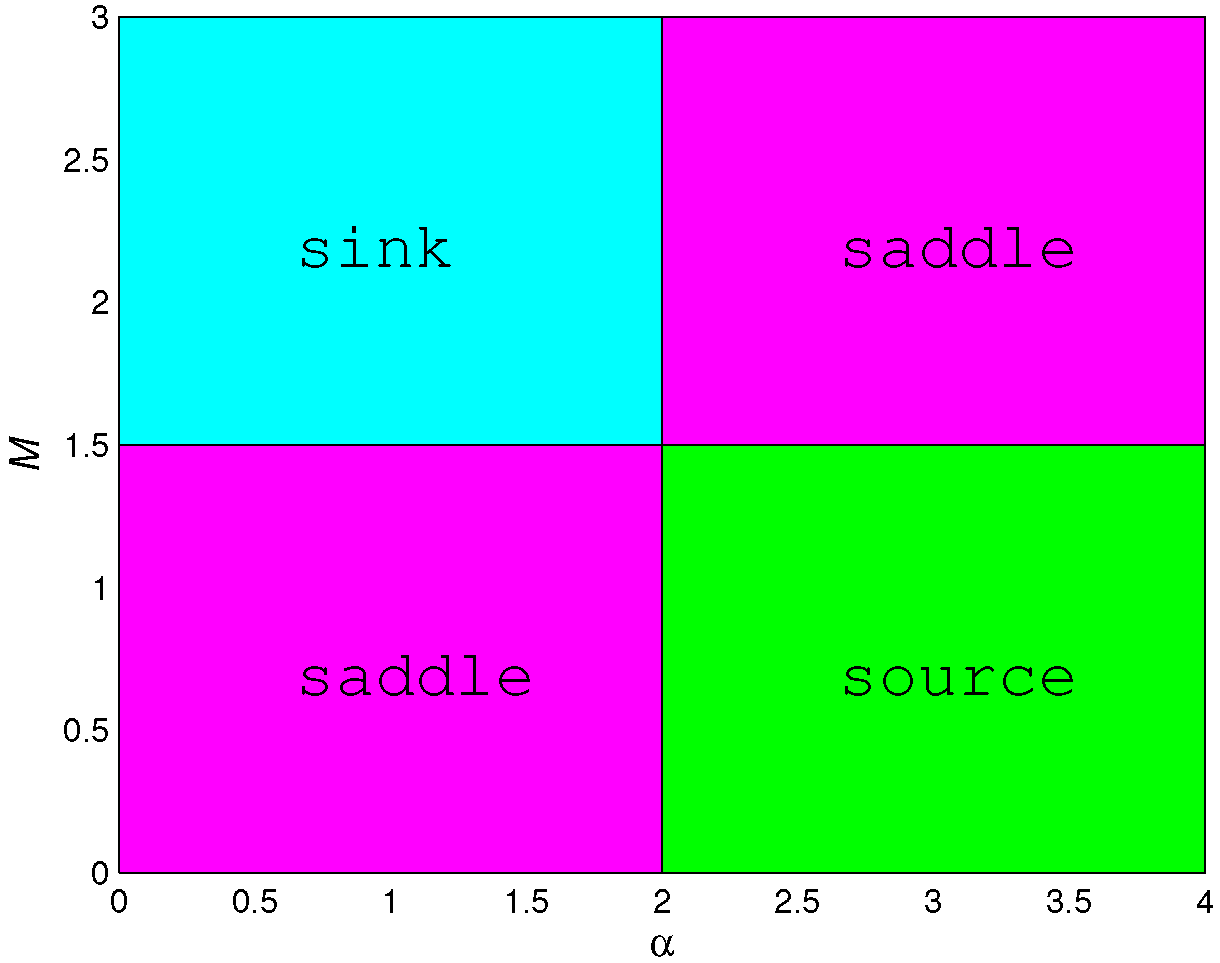
(1) 

A sink if $|{\lambda }_1| <1$ and $|{\lambda }_2| <1,$ and it is locally asymptotically stable;

(2) 

A source if $|{\lambda }_1| >1$ and $|{\lambda }_2| >1,$ and it is unstable;

(3) 

A saddle if $|{\lambda }_1| >1$ and $|{\lambda }_2| <1$ (or $|{\lambda }_1| <1$ and $|{\lambda }_2| >1);$

(4) 

Non-hyperbolic if either $\left|{\lambda }_1\right| =1or|{\lambda }_2| =1$.

Now, using Definition 1, we topologically categorize fixed points and discuss their local stability.

Note that, when $M=0$,

$$J\left(E_0\right)=\left(\begin{array}{cc}{\displaystyle e^{\alpha }}& {\displaystyle 0}\\ {\displaystyle 0}& {\displaystyle \mathrm{e}}\end{array}\right),J\left(E_1\right)=\left(\begin{array}{cc}{\displaystyle 1-\alpha }& \alpha \beta \\ 0& {\displaystyle \mathrm{e}}\end{array}\right),$$

and for the case $M>0$,

$$J\left(E_0\right)=\left(\begin{array}{cc}{\mathrm{e}}^{\alpha }& 0\\ 0& {\mathrm{e}}^{1-\frac{M}{A}}\end{array}\right),J\left(E_1\right)=\left(\begin{array}{cc}1-\alpha & \alpha \beta \\ 0& {\mathrm{e}}^{1-\frac{M}{A}}\end{array}\right).$$

Thus, the following conclusion can be drawn.

Theorem 4.

Assume that $M=0,$ and we have the following description:

(1) 

$E_0(0,0)$ is always a source since two eigenvalues are ${\mathrm{e}}^{\alpha }>1$ and $\mathrm{e}>1.$

(2) 

Two eigenvalues of $E_1(\alpha ,0)$ are $1-\alpha <1$ and $\mathrm{e}>1$. Then, $E_1(\alpha ,0)$ is:

(i) 

A saddle when $0<\alpha <2;$

(ii) 

A source when $\alpha >2;$

(iii) 

Non-hyperbolic when $\alpha =2.$

By Theorem 4(iii), the two eigenvalues of $J\left(E_1\right)$ are ${\lambda }_1=-1,{\lambda }_2=e$; hence, $E_1$ is non-hyperbolic. The conditions that satisfy Theorem 4(iii) for the set ${\Omega }_{E_f}$ are written as follows:

$${\Omega }_{{\mathit{E}}_{\mathit{f}}}=\{(\alpha ,\beta )\in {\mathbb{R}}^2:\alpha =2,\beta >0\}.$$

Choose the bifurcation parameter $\alpha$, and set it to $\alpha =2+\rho$. A suitably tiny perturbation term is $\rho$. According to a quick calculation, the center manifold of the map (5) in ${\Omega }_{E_f}$ is $y=0$. In this instance, the map (5) may be expressed as $x\to -x-\rho x+\frac{1}{6}{x}^3+\frac{1}{2}\rho x^2+O\left({(\left|x\right|+\left|\rho \right|)}^3\right)$. As a result, at $E_1$, a flip bifurcation is formed.

Figure 3 depicts the bifurcation diagram of the numerical simulation for $\beta =0,\alpha \in [0,4]$, and $x\in [0,20]$. Figure 3 shows that, when $0<\alpha <2$, the shape of the map (5) is stable; when $\alpha >2$, the map (5) turns over due to instability and provides stable biperiodic solutions. A chaotic set is produced as $\alpha$ rises.

Figure 3. Flip bifurcation diagrams of commensal species at initial value $(x_0,y_0)=(0.5,0.3)$ with $M=0$ and $\alpha \in [0,4]$.

Theorem 5.

Assume that $M>0$; in this case, the two eigenvalues of the map (5) at fixed point $E_0(0,0)$ are $e^{\alpha }$ and $e^{1-\frac{A}{M}},$then $E_0(0,0)$ is:

(1) 

A source if $0<M<A;$

(2) 

A saddle if $M>A;$

(3) 

Non-hyperbolic if $M=A$.

Theorem 6.

The two eigenvalues of the map (5) at the fixed point $E_1\left(\alpha ,0\right)$ are $1-\alpha$ and $e^{1-\frac{A}{M}}$; consequently, $E_1(\alpha ,0)$ is:

(1) 

A sink if and only if $0<\alpha <2$ and $M>A$;

(2) 

A source if and only if $\alpha >2$ and $0<M<A$;

(3) 

A saddle if and only if $0<\alpha <2$ and $0<M<A$ or $\alpha >2$ and $M>A$;

(4) 

Non-hyperbolic if $M=A$ or $\alpha =2$.

Proof. 

At the boundary fixed point $E_1(\alpha ,0)$, whose eigenvalues are $1-\alpha <1$ and $e^{1-\frac{A}{M}}>0,$ it is simple to see that

$$1-\alpha \left\{\begin{array}{cc}>-1\hfill & \mathrm{if} 0<\alpha <2,\hfill \\ =-1\hfill & \mathrm{if} \alpha =2,\hfill \\ <-1\hfill & \mathrm{if} \alpha >2.\hfill \end{array}\right.$$

and

$$e^{1-\frac{A}{M}}\left\{\begin{array}{cc}>1\hfill & \mathrm{if} 0<M<A,\hfill \\ =1\hfill & \mathrm{if} M=A,\hfill \\ \in \left(0,1\right)\hfill & \mathrm{if} M>A.\hfill \end{array}\right.$$

Then, the result follows. □

Figure 4 displays the topological classification of the map (5) at boundary fixed point $E_1(\alpha ,0)$ when $\beta =1,A=1.5,\alpha \in [0,4]$, and $M\in [0,3]$.

Figure 4. Topological classification at $E_1(\alpha ,0)$ with $\beta =1,A=1.5,\alpha \in [0,4]$, and $M\in [0,3]$.

Now, we give the Jacobian matrix of the map (5) at the boundary fixed points $E_{2i}\left(0,y_i^{}\right)\left(i=1,2,3\right)$ as follows:

$$J\left(E_{2i}\right)=\left(\begin{array}{cc}{\mathrm{e}}^{\alpha +\beta y_i}& 0\\ 0& J_i\end{array}\right),$$

where $J_i=1+y_i\left(-1+\frac{M}{{(y_i+A)}^2}\right)$. Clearly, the two eigenvalues of $J\left(E_{2i}\right)$ are $e^{\alpha +\beta y_i}>1$ and $J_i$. Note that $J_i$ was analyzed in Section 2.2. Then, we have $J_1>1,J_2\in (-1,1)$ and $J_3=1$. Thus, we obtain the following conclusions:

Theorem 7.

(1) 

When $A<M<M^{*}$ and $0<A<1,$ the boundary fixed point $E_{21}$ exists in the map (5), and the eigenvalues of $J\left(E_{21}\right)$ are $e^{\alpha +\beta y_1}>1$ and $J_1>1$. So, the fixed point $E_{21}$ is always a source.

(2) 

When the boundary fixed point $E_{22}$ exists, the eigenvalues of $J\left(E_{22}\right)$ are $e^{\alpha +\beta y_2}>1$ and $|J_2|<1$. So, the fixed point $E_{22}$ is always a saddle.

(3) 

When $M=M^{*}$ and $0<A<1,$ the boundary fixed point $E_{23}$ exists in the map (5), and the eigenvalues of $J\left(E_{23}\right)$ are $e^{\alpha +\beta y_3}>1$ and $J_3=1.$ Consequently, $E_{23}$ is always non-hyperbolic.

Next, the Jacobian matrix at positive points $E_{3i}^{*}\left(x_i^{*},y_i\right)\left(i=1,2,3\right)$ is obtained as

$$J\left(E_{3i}^{*}\right)=\left(\begin{array}{cc}1-x_i^{*}& \beta x_i^{*}\\ 0& J_i\end{array}\right),$$

where $x_i^{*}=\alpha +\beta y_i$, whose eigenvalues are $1-x_i^{*}<1$, and $J_i$ was analyzed above. Then, we obtain

$$1-x_i^{*}\left\{\begin{array}{cc}>-1\hfill & \mathrm{if} 0<x_i^{*}<2,\hfill \\ =-1\hfill & \mathrm{if} x_i^{*}=2,\hfill \\ <-1\hfill & \mathrm{if} x_i^{*}>2.\hfill \end{array}\right.$$

This is equivalent to the following two situations.

(1)

If $0<\alpha <2$, we have

$$x_i^{*}\left\{\begin{array}{cc}<2\hfill & \mathrm{if} 0<\beta <{\beta }_i^{*},\hfill \\ =2\hfill & \mathrm{if} \beta ={\beta }_i^{*},\hfill \\ >2\hfill & \mathrm{if} \beta >{\beta }_i^{*}.\hfill \end{array}\right.$$

where ${\beta }_i^{*}=\frac{2-\alpha }{y_i},(i=1,2,3).$

(2)

If $\alpha \ge 2$, we have $1-x_i^{*}<-1$, which is equivalent to $x_i^{*}>2$.

As a consequence of the above analysis, we have:

Theorem 8.

(1) 

When $E_{31}^{*}(x_{31}^{*},y_1)$ exists, it is:

(i) 

A saddle if and only if $0<\alpha <2$ and $0<\beta <{\beta }_1^{*}$;

(ii) 

A source if and only if $0<\alpha <2$ and $\beta >{\beta }_1^{*}$ or $\alpha >2$;

(iii) 

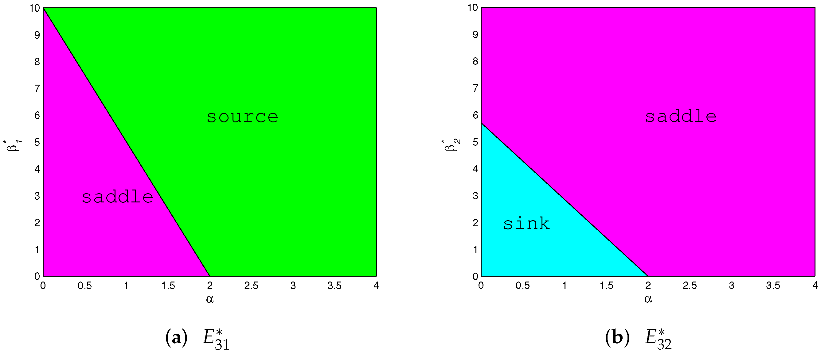
Non-hyperbolic if and only if $0<\alpha <2$ and $\beta ={\beta }_1^{*}$, where ${\beta }_1^{*}=\frac{2-\alpha }{y_1}.$

(2) 

When $E_{32}^{*}(x_{32}^{*},y_2)$ exists, it is:

(i) 

A sink if and only if $0<\alpha <2$ and $0<\beta <{\beta }_2^{*}$;

(ii) 

A saddle if and only if $0<\alpha <2$ and $\beta >{\beta }_2^{*}$ or $\alpha >2$;

(iii) 

Non-hyperbolic if and only if $0<\alpha <2$ and $\beta ={\beta }_2^{*}$, where ${\beta }_2^{*}=\frac{2-\alpha }{y_2}.$

(3) 

When $E_{33}^{*}(x_{33}^{*},y_3)$ exists and $0<\alpha <2$, it is always non-hyperbolic, where ${\beta }_3^{*}=\frac{2-\alpha }{y_3}.$

When $M=0.52,A=0.45,\alpha \in [0,4]$ and ${\beta }_i^{*}\in [0,10],$ Figure 5 shows the topological classification of the map (5) at positive fixed points $E_{3i}(x_i^{*},y_i)(i=1,2)$.

Figure 5. Topological classification of the $\alpha -{\beta }_i^{*}$ plane at $E_{3i}(x_i^{*},y_i)$ with $M=0.52,A=0.45$, $\alpha \in [0,4]$, and ${\beta }_i^{*}\in [0,10],(i=1,2)$.

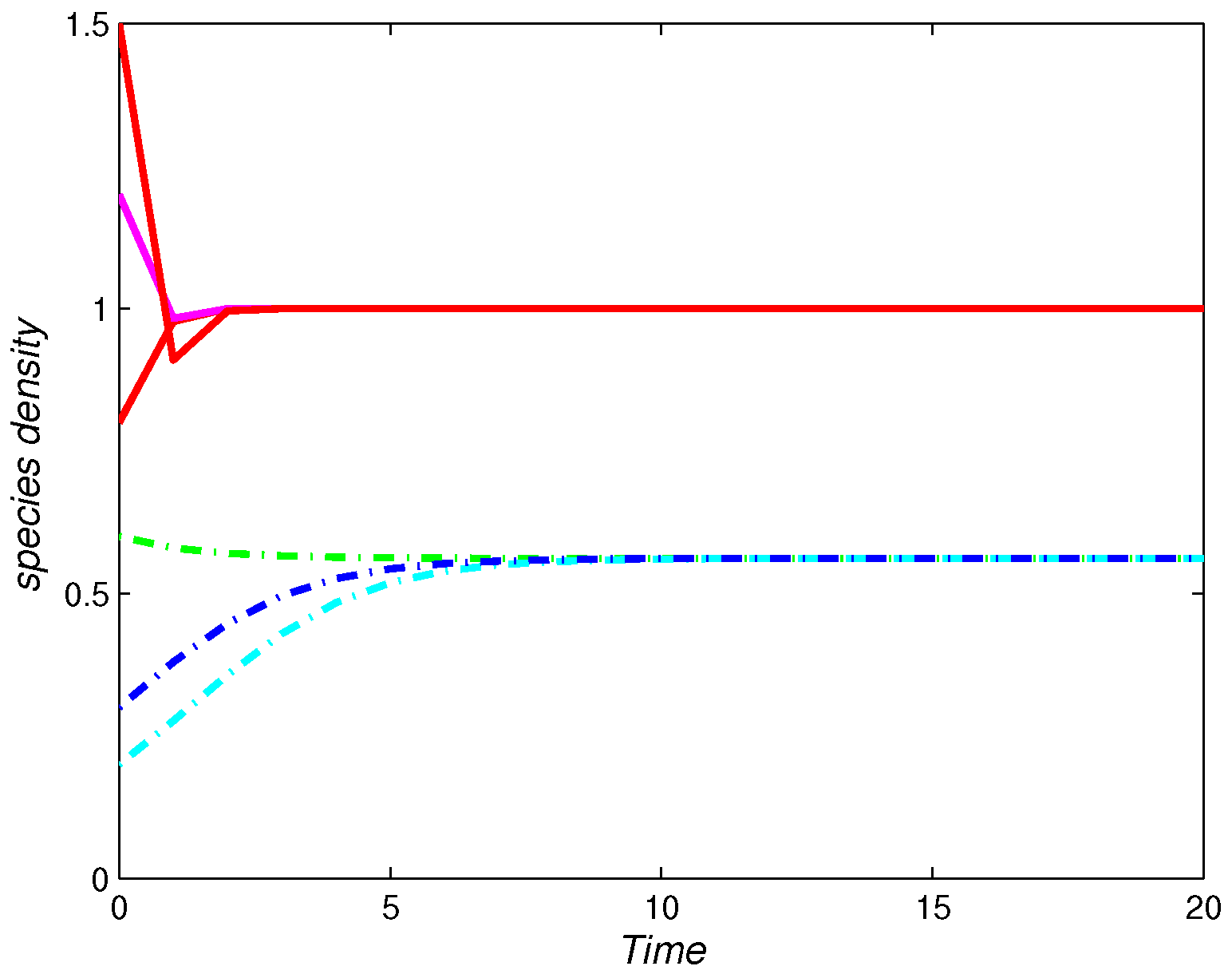
3.2. Global Stability of Positive Fixed Point $E_{32}^{*}$

Firstly, we give two lemmas in [37].

Lemma 1.

Suppose that the sequences $x\left(n\right)$ satisfy $x\left(n\right)>0$ and

$$x(n+1)\le x\left(n\right)exp\left(a-bx\left(n\right)\right),n\in \mathbb{N},$$

where a and b are positive constants. Then,

$$\underset{n\to +\infty }{lim\; sup}x\left(n\right)\le \frac{exp(a-1)}{b}:=M.$$

Lemma 2.

Suppose that the sequences $x\left(n\right)$ satisfy $x\left(n\right)>0$ and

$$x(n+1)\ge x\left(n\right)exp\left(a-bx\left(n\right)\right),n\in \mathbb{N},$$

where a and b are positive constants. Then,

$$\underset{n\to +\infty }{lim\; inf}x\left(n\right)\ge \frac{a}{b}exp\left(a-bM\right),$$

where M was given by Lemma 2.

Secondly, from Theorem 2, we obtain that, if $0<M<AorM=A,0<A<1$ holds, $y\left(n\right)$ is any positive solution of the map (6), then

$$\underset{n\to \infty }{lim}y\left(n\right)=y_2.$$

(8)

Now, we consider a system as follows:

$$x_1(n+1)=x_1\left(n\right)exp\left(\alpha +\beta y_2-x_1\left(n\right)\right),$$

(9)

where $x_1\left(n\right)=\alpha +\beta y_2$ is any positive solution of System (9). We obtain the following result.

Theorem 9.

If

$$\begin{array}{c}\hfill 0<M<A,or(M=A,0<A<1)and0<\alpha +\beta y_2<ln2+1\end{array}$$

(10)

holds, the positive fixed point $E_{32}^{*}(x_2^{*},y_2)$ of the map (5) is globally attractive. In other words,

$$\underset{n\to +\infty }{lim}[x\left(n\right)-x_1\left(n\right)]=0,$$

where $x_1\left(n\right)$ is any positive solution of System (9).

Proof. 

From (8), for any sufficiently small $\epsilon >0$, there is an integer $N_1$ such that, if $n>N_1$, then

$$y_2-\epsilon <y_n<y_2+\epsilon .$$

(11)

In order to prove ${lim}_{n\to +\infty }[x\left(n\right)-x_1\left(n\right)]=0,$ let

$$x\left(n\right)=x_1\left(n\right)exp\left[k\left(n\right)\right].$$

Then, by using the differential mean value theorem, the first equation of (5) can be expressed as

$$\begin{array}{ccc}k(n+1)\hfill & =\hfill & lnx\left(n\right)+\alpha -x\left(n\right)+\beta y\left(n\right)-ln{x}_1(n+1)\hfill \\ \hfill & =\hfill & k\left(n\right)(1-x_1\left(n\right)exp\left[\theta \left(n\right)k\left(n\right)\right])+\beta (y_n-y_2),\hfill \end{array}$$

(12)

where $\theta \left(n\right)\in [0,1]$, and $x_1\left(n\right)exp\left[{\theta }_1\left(n\right)k\left(n\right)\right]$ lies in the range of $x_1\left(n\right)$ to $x\left(n\right)$. Now, our primary purpose is to prove

$$\underset{n\to +\infty }{lim}{k}_1\left(n\right)=0.$$

because of $x\left(n\right)exp\left[\alpha +\beta (y_2-\epsilon )-x\left(n\right)\right]\le x(n+1)\le x\left(n\right)exp\left[\alpha +\beta (y_2+\epsilon )-x\left(n\right)\right],$ then with the help of Lemmas 1 and 2, we obtain

$$\begin{array}{cc}\hfill \underset{n\to +\infty }{lim\; sup}x\left(n\right)& \le exp\left(\alpha +\beta (y_2+\epsilon )-1\right):=U_1,\hfill \\ \hfill \underset{n\to +\infty }{lim\; inf}x\left(n\right)& \ge (\alpha +\beta (y_2+\epsilon ))exp\left[\alpha +\beta (y_2+\epsilon )-U_1\right]\hfill \\ \hfill & \ge (\alpha +\beta (y_2-\epsilon ))exp\left[\alpha +\beta (y_2-\epsilon )-U_1\right]:=V_1.\hfill \end{array}$$

In addition, from (9), Lemmas 1 and 2, we obtain

$$\begin{array}{cc}\hfill \underset{n\to +\infty }{lim\; sup}{x}_1\left(n\right)& \le exp[\alpha +\beta y_2-1]:=U_2\le U_1,\hfill \\ \hfill \underset{n\to +\infty }{lim\; inf}{x}_1\left(n\right)& \ge (\alpha +\beta y_2)exp\left[\alpha +\beta y_2-U_2\right]\hfill \\ \hfill & \ge (\alpha +\beta y_2)exp\left[\alpha +\beta y_2-U_1\right]\hfill \\ \hfill & \ge (\alpha +\beta (y_2-\epsilon )exp\left[\alpha +\beta (y_2-\epsilon )-U_1\right]:=V_1.\hfill \end{array}$$

Thus, for any sufficiently small $\epsilon >0$, there is an integer $N_2>N_1$ such that, if $n\ge N_2$, then

$$V_1-\epsilon \le x\left(n\right),x_1\left(n\right)\le U_1+\epsilon ,n\ge N_2.$$

(13)

Suppose that

$$\lambda =max\left\{|1-V_1|,|1-U_1|\right\}.$$

Then, for any sufficiently small $\epsilon >0$, we suppose

$${\lambda }_{\epsilon }=max\left\{|1-(V_1-\epsilon )|,|1-(U_1+\epsilon )|\right\}.$$

(14)

From (11)–(14), we obtain

$$\begin{array}{cc}\hfill \left|k\right(n+1\left)\right|& \le max\left\{|1-(V_1-\epsilon )|,|1-(U_1+\epsilon )|\right\}\left|k\left(n\right)\right|+\beta \epsilon \hfill \\ \hfill & ={\lambda }_{\epsilon }+\beta \epsilon ,n\ge N_2.\hfill \end{array}$$

Then, we obtain the following inequality:

$$\left|k\left(n\right)\right|\le {\lambda }_{\epsilon }^{n-N_2}\left|k\left(N_2\right)\right|+\frac{1-{\lambda }_{\epsilon }^{n-N_2}}{1-{\lambda }_{\epsilon }}\beta \epsilon ,n\ge N_2.$$

(15)

Since ${\lambda }_{\epsilon }<1$ and $\epsilon$ is sufficiently small, we can have ${lim}_{n\to +\infty }k\left(n\right)=0$, i.e., ${lim}_{n\to +\infty }\left[x\left(n\right)-x_1\left(n\right)\right]=0$ holds when ${\lambda }_1<1$. Notice that

$$1-U_1<1-V_1<1,$$

then ${\lambda }_1<1$ is equivalent to

$$1-U_1>-1,$$

i.e.,

$$0<\alpha +\beta (y_2+\epsilon )<1+ln2.$$

(16)

Since $\epsilon$ is sufficiently small when (10) holds, we obtain (16), so ${lim}_{n\to +\infty }\left[x\left(n\right)-x_1\left(n\right)\right]=0$. Thus, this completes the proof of Theorem 9. □

3.3. Bifurcation Analysis of a Codimension of One

According to the prior analysis of the map (5) at fixed points, in this section, the center manifold theorem is used to reduce dimensionality, and then, bifurcation theory is employed to investigate the bifurcations of a codimension of one at non-hyperbolic fixed points by [44,45].

3.3.1. Bifurcation at the Fixed Point $E_0(0,0)$

Theorem 10.

When parameters $(\alpha ,\beta ,M,A)\in {\Omega }_{\mathit{E}0}=\{(\alpha ,\beta ,M,A)\in {\mathbb{R}}^4:\alpha >0,\beta >0,M=A,A>0\}$, $E_0$ is a non-hyperbolic fixed point. Furthermore, we find that the map (5) will undergo:

(1) 

A transcritical bifurcation when parameters $(\alpha ,\beta ,M,A)\in {\Omega }_{\mathit{E}{0}_{\mathit{TR}}}=\{(\alpha ,\beta ,M,A)\in {\mathbb{R}}^4:\alpha >0,\beta >0,M=A,A\ne 1\}$ hold;

(2) 

A pitchfork bifurcation when $(\alpha ,\beta ,M,A)\in {\Omega }_{\mathit{E}{0}_{\mathit{PF}}}=\{(\alpha ,\beta ,M,A)\in {\mathbb{R}}^4:\alpha >0,\beta >0,M=A=1\}$ holds.

Proof. 

By Theorem 5, the two eigenvalues of $J\left(E_0\right)$ are ${\lambda }_1=e^{\alpha }>1,{\lambda }_2=1$, and the fixed point $E_0$ is called non-hyperbolic if $(\alpha ,\beta ,M,A)\in {\Omega }_{\mathit{E}0}$. We choose M as the bifurcation parameter, and $\rho$ is the perturbation parameter near A, satisfying $M=A+\rho$. Then, through an iterative operation, we can easily calculate that the center manifold of the map (5) is given as $x=0$ and that the constrained map (5) can be represented as $y\to y-\frac{(A-1)}{A}{y}^2-\frac{1}{A}y\rho +\frac{(A^2-2A-1)}{2A^2}{y}^3+\frac{1}{A}{y}^2\rho +\frac{1}{2A^2}y{\rho }^2+O\left({(\left|y\right|+\left|\rho \right|)}^3\right)$. If $(\alpha ,\beta ,M,A)\in {\Omega }_{\mathit{E}{0}_{\mathit{TR}}}=\{(\alpha ,\beta ,M,A)\in {\mathbb{R}}^4:\alpha >0,\beta >0,M=A,A\ne 1\}$ holds, thus the map (5) undergoes a transcritical bifurcation at $E_0(0,0)$; if $(\alpha ,\beta ,M,A)\in {\Omega }_{\mathit{E}{0}_{\mathit{PF}}}=\{(\alpha ,\beta ,M,A)\in {\mathbb{R}}^4:\alpha >0,\beta >0,M=A=1\}$, then the map (5) undergoes a pitchfork bifurcation at $E_0(0,0)$. □

3.3.2. Bifurcation around Boundary Fixed Point $E_1(\alpha ,0)$

Theorem 11.

The map (5) at $E_1(\alpha ,0)$ has:

(i) 

A transcritical bifurcation or a pitchfork bifurcation, whose boundary fixed point $E_1(\alpha ,0)$ is non-hyperbolic, if parameter $(\alpha ,\beta ,M,A)\in {\Omega }_{\mathit{E}{1}_{\mathit{TR}}}=\{(\alpha ,\beta ,M,A)\in {\mathbb{R}}^4:\alpha \ne 2,\beta >0,M=A,A\ne 1\}$ or ${\Omega }_{\mathit{E}{1}_{\mathit{PF}}}=\{(\alpha ,\beta ,M,A)\in {\mathbb{R}}^4:\alpha \ne 2,$ $\beta >0,M=A=1\}$, respectively;

(ii) 

A flip bifurcation if $(\alpha ,\beta ,M,A)\in {\Omega }_{\mathit{E}{1}_{\mathit{FB}}}=\{(\alpha ,\beta ,M,A)\in {\mathbb{R}}^4:\alpha =2,\beta >0,M\ne A,A>0\}$.

Proof. 

$\left(i\right)$According to Theorem 6(4), when the parameters satisfy the conditions $(\alpha ,\beta ,$$M,A)\in {\Omega }_{\mathit{E}{1}_{\mathit{TR}}}=\{(\alpha ,\beta ,M,A)\in {\mathbb{R}}^4:\alpha \ne 2,\beta >0,M=A,A\ne 1\}$, one eigenvalue of the Jacobian matrix $J\left(E_1\right)$ is $1-\alpha$ and the other is 1. First, we choose M as the bifurcation parameter. Set $\mu =M-A$, where $\left|\mu \right|\ll 1$, and it is a new variable. Next, we translate System (5) to the originwith $u=x-\alpha ,v=y-0$ and perform the Taylor expansion, leading to

$$\left(\begin{array}{c}{\displaystyle u}\\ {\displaystyle v}\end{array}\right)\to \left(\begin{array}{cc}1-\alpha & \alpha \beta \\ 0& 1\end{array}\right)\left(\begin{array}{c}{\displaystyle u}\\ {\displaystyle v}\end{array}\right)+\left(\begin{array}{c}{\displaystyle f_1(u,v,\mu )}\\ {\displaystyle f_2(u,v,\mu )}\end{array}\right);$$

(17)

here,

$$\begin{array}{cc}\hfill f_1(u,v,\mu )& =z_{11}uv+z_{20}{u}^2+z_{02}{v}^2+z_{21}{u}^{2}v+z_{12}u{v}^2+z_{30}{u}^3\hfill \\ \hfill & + z_{03}{v}^3+O\left({(\left|u\right|+\left|v\right|+\left|\mu \right|)}^3\right),\hfill \\ \hfill f_2(u,v,\mu )& =b_{20}{v}^2+b_{11}v\mu +b_{30}{v}^3+b_{21}{v}^2\mu +b_{12}v{\mu }^2\hfill \\ \hfill & + O\left({(\left|u\right|+\left|v\right|+\left|\mu \right|)}^3\right),\hfill \end{array}$$

and

$$\begin{array}{cc}\hfill z_{11}& =-(\alpha -1)\beta ,z_{20}=\frac{(\alpha -2)}{2},z_{02}=\frac{\alpha {\beta }^2}{2},\hfill \\ \hfill z_{21}& =\frac{(\alpha -2)\beta }{2},z_{12}=-\frac{(\alpha -1){\beta }^2}{2},z_{30}=-\frac{(\alpha -3)}{6},\hfill \\ \hfill z_{03}& =-\frac{\alpha {\beta }^3}{6},b_{20}=-\frac{(A-1)}{A},b_{11}=-\frac{1}{A},\hfill \\ \hfill b_{30}& =\frac{(A^2-2A-1)}{2A^2},b_{21}=\frac{1}{A},b_{12}=\frac{1}{2A^2}.\hfill \end{array}$$

The matrix of the linear part of the map (17) can be expressed as:

$$J\left(E_1\right)=\left(\begin{array}{cc}1-\alpha & \alpha \beta \\ 0& 1\end{array}\right).$$

Choose invertible matrix T:

$$T=\left(\begin{array}{cc}1& \beta \\ 0& 1\end{array}\right).$$

Apply the following matrix transformation to the map (17):

$${\displaystyle \left(\begin{array}{c}{\displaystyle u}\\ {\displaystyle v}\end{array}\right)=T\left(\begin{array}{c}{\displaystyle U}\\ {\displaystyle V}\end{array}\right).}$$

(18)

Therefore, the map (17) becomes

$$\left(\begin{array}{c}{\displaystyle U}\\ {\displaystyle V}\end{array}\right)\to \left(\begin{array}{cc}1-\alpha & 0\\ 0& 1\end{array}\right)\left(\begin{array}{c}{\displaystyle U}\\ {\displaystyle V}\end{array}\right)+\left(\begin{array}{c}{\displaystyle G_1(U,V,\mu )}\\ {\displaystyle G_2(U,V,\mu )}\end{array}\right),$$

(19)

where

$$\begin{array}{cc}\hfill G_1(U,V,\mu )& =z_{20}{U}^2+\left(2\beta z_{20}+z_{11}\right)UV+\left(z_{20}{\beta }^2-b_{20}\beta +z_{11}\beta +z_{02}\right)V^2\hfill \\ \hfill & - \beta b_{11}V\mu +(3\beta z_{30}+z_{21})U^{2}V+(3{\beta }^2{z}_{30}+2\beta z_{21}+z_{12})U{V}^2\hfill \\ \hfill & + z_{30}{U}^3+\left(z_{30}{\beta }^3+z_{21}{\beta }^2-b_{30}\beta +z_{12}\beta +z_{03}\right)V^3-b_{12}\beta V{\mu }^2\hfill \\ \hfill & - b_{21}\beta V^2\mu +O\left({(\left|U\right|+\left|V\right|+\left|\mu \right|)}^3\right),\hfill \\ \hfill G_2(U,V,\mu )& =b_{20}{V}^2+b_{11}V\mu +b_{30}{V}^3+b_{21}{V}^2\mu +b_{12}V{\mu }^2+O\left({(\left|U\right|+\left|V\right|+\left|\mu \right|)}^3\right).\hfill \end{array}$$

Then, to study the stability of $(U,V)=(0,0)$ near $\mu =0$, we can indirectly study a system of one-parameter equations limited to a center manifold. It can be defined as follows:

$$W^c(0,0,0)=\left\{(U,V,\mu )\in {\mathbb{R}}^3:U=g(V,\mu ),g(0,0)=0,Dg(0,0)=0\right\}$$

with V and $\mu$ small. Take

$$g(V,\mu )=g_1{\mu }^2+g_{2}V\mu +g_3{V}^2+O\left(\right(\left|V\right|+{\left|\mu \right|)}^3).$$

(20)

Then, we have

$$N\left(g(V,\mu )\right)=g(V+G_2(g(V,\mu ),V,\mu ),\mu )-(1-\alpha )g(V,\mu )-G_1(g(V,\mu ),V,\mu ))=0.$$

(21)

Substituting (20) into (21) and comparing the coefficients of ${\mu }^2,V\mu$ and $V^2$ of (21), we obtain

$$g_1=0,g_2=\frac{\beta }{\alpha A},g_3=\frac{\beta (A-1)}{A\alpha }.$$

Thus, the map restricted to the center manifold $W^c(0,0,0)$ is written as

$$F_1:V\to V+b_{20}{V}^2+b_{11}V\mu +b_{30}{V}^3+b_{21}{V}^2\mu +b_{12}V{\mu }^2+O\left(\right(\left|V\right|+{\left|\mu \right|)}^3).$$

We can see that

$$\begin{array}{cc}\hfill & F_1(0,0)=0,\frac{\partial F_1}{\partial V}(0,0)=1,\frac{\partial F_1}{\partial \mu }(0,0)=0,\hfill \\ \hfill & \frac{{\partial }^2{F}_1}{\partial V\partial \mu }(0,0)=b_{11}=-\frac{1}{A}\ne 0,\frac{{\partial }^2{F}_1}{\partial V^2}(0,0)=2b_{20}=-\frac{2(A-1)}{A}.\hfill \end{array}$$

Hence, the map (5) undergoes a transcritical bifurcation at $E_1$ because of $\frac{{\partial }^2{F}_1}{\partial V^2}(0,0)\ne 0$ if $(\alpha ,\beta ,M,A)\in {\Omega }_{\mathit{E}{1}_{\mathit{TR}}}$. Moreover, when $(\alpha ,\beta ,M,A)\in {\Omega }_{\mathit{E}{1}_{\mathit{PF}}}=\{(\alpha ,\beta ,M,A)\in {\mathbb{R}}^4:\alpha \ne 2,$ $\beta >0,M=A=1\}$, a direct calculation leads to $\frac{{\partial }^2{F}_1}{\partial V^2}(0,0)=0$ and $\frac{{\partial }^3{F}_1}{\partial V^3}(0,0)=-6$; from [45] the map (5) will pass through a pitchfork bifurcation at $E_1$.

$\left(ii\right)$ From Theorem 6(4), when $(\alpha ,\beta ,M,A)\in {\Omega }_{\mathit{E}{1}_{\mathit{FB}}}=\{(\alpha ,\beta ,M,A)\in {\mathbb{R}}^4:\alpha =2,$ $\beta >0,M\ne A,A>0\}$ holds, it is evident that, for the non-hyperbolic $E_1(\alpha ,0)$, ${\lambda }_1=-1$ and ${\lambda }_2=exp(1-\frac{M}{A})\ne 1$. Taking $\alpha$ as a bifurcation parameter and assuming $\epsilon$ that is a sufficiently small perturbation parameter, namely $∥\epsilon ∥\ll 1$, then, the perturbations corresponding to System (5) are mapped as follows:

$$\left(\begin{array}{c}{\displaystyle x}\\ {\displaystyle y}\end{array}\right)\to \left(\begin{array}{c}{\displaystyle x{\mathrm{e}}^{2+\epsilon -x+\beta y}}\\ {\displaystyle y{\mathrm{e}}^{1-y-\frac{M}{y+A}}}\end{array}\right).$$

(22)

Then, we shift $E_1$ in the map (12) to (0,0) using a transformation $u=x-(2+\epsilon ),v=y-0$, which leads to

$$\left(\begin{array}{c}{\displaystyle u}\\ {\displaystyle v}\end{array}\right)\to \left(\begin{array}{cc}{\displaystyle -1}& {\displaystyle 2\beta }\\ {\displaystyle 0}& {\displaystyle {\lambda }_2}\end{array}\right)\left(\begin{array}{c}{\displaystyle u}\\ {\displaystyle v}\end{array}\right)+\left(\begin{array}{c}{\displaystyle f_3(u,v,\epsilon )}\\ {\displaystyle f_4(u,v,\epsilon )}\end{array}\right);$$

(23)

here,

$$\begin{array}{cc}\hfill f_3(u,v,\epsilon )& ={\beta }^2{v}^2-\beta uv+\beta v\epsilon -u\epsilon +\frac{1}{6}{u}^3+\frac{1}{2}{u}^2\epsilon -\beta uv\epsilon -\frac{1}{2}{\beta }^{2}u{v}^2\hfill \\ \hfill & + \frac{1}{3}{\beta }^3{v}^3+\frac{1}{2}{\beta }^2{v}^2\epsilon +O\left({(\left|u\right|+\left|v\right|+\left|\epsilon \right|)}^3\right),\hfill \\ \hfill f_4(u,v,\epsilon )& =-\frac{(A^2-M){\lambda }_2}{A^2}{v}^2+\frac{(A^4-2M{A}^2-2MA+M^2){\lambda }_2}{2A^4}{v}^3\hfill \\ \hfill & + O\left({(\left|u\right|+\left|v\right|+\left|\epsilon \right|)}^3\right).\hfill \end{array}$$

Taking the map (23) at origin $(0,0)$, the Jacobian matrix is

$$J\left(E_1\right)=\left(\begin{array}{cc}{\displaystyle -1}& {\displaystyle 2\beta }\\ {\displaystyle 0}& {\displaystyle {\lambda }_2}\end{array}\right).$$

Invertible matrices T are constructed as follows:

$$T=\left(\begin{array}{c}\begin{array}{cc}1& \frac{2\beta }{1+{\lambda }_2}\\ 0& 1\end{array}\end{array}\right).$$

With the transformation

$${\displaystyle \left(\begin{array}{c}{\displaystyle u}\\ {\displaystyle v}\end{array}\right)=T\left(\begin{array}{c}{\displaystyle X}\\ {\displaystyle Y}\end{array}\right),}$$

(24)

the map (23) becomes

$$\left(\begin{array}{c}{\displaystyle X}\\ {\displaystyle Y}\end{array}\right)\to \left(\begin{array}{cc}-1& 0\\ 0& {\lambda }_2\end{array}\right)\left(\begin{array}{c}{\displaystyle X}\\ {\displaystyle Y}\end{array}\right)+\left(\begin{array}{c}{\displaystyle G_3(X,Y,\epsilon )}\\ {\displaystyle G_4(X,Y,\epsilon )}\end{array}\right),$$

(25)

where

$$\begin{array}{cc}\hfill G_3(X,Y,\epsilon )& =-\beta XY-X\epsilon +\left({\beta }^2-\frac{2{\beta }^2}{1+{\lambda }_2}+\frac{2\beta {\lambda }_2(A^2-M)}{A^2(1+{\lambda }_2)}\right)Y^2+\left(\beta -\frac{2\beta }{1+{\lambda }_2}\right)Y\epsilon \hfill \\ \hfill & + \frac{1}{6}{X}^3+\frac{\beta }{1+{\lambda }_2}{X}^{2}Y+\left(\frac{2{\beta }^2}{{(1+{\lambda }_2)}^2}-\frac{{\beta }^2}{2}\right){\mathit{XY}}^2+\left(\frac{2\beta }{1+{\lambda }_2}-\beta \right)XY\epsilon \hfill \\ \hfill & + \left(\frac{4{\beta }^3}{3{(1+{\lambda }_2)}^3}-\frac{{\beta }^3}{1+{\lambda }_2}+\frac{{\beta }^3}{3}-\frac{\beta {\lambda }_2(A^4-2A^{2}M-2AM+M^2)}{A^4(1+{\lambda }_2)}\right)Y^3\hfill \\ \hfill & + \frac{1}{2}{X}^2\epsilon +\left(\frac{2{\beta }^2}{{(1+{\lambda }_2)}^2}-\frac{2{\beta }^2}{1+{\lambda }_2}+\frac{{\beta }^2}{2}\right)Y^2\epsilon +O\left({(\left|X\right|+\left|Y\right|+\left|\epsilon \right|)}^3\right),\hfill \\ \hfill G_4(X,Y,\epsilon )& =-\frac{(A^2-M){\lambda }_2}{A^2}{V}^2+\frac{(A^4-2A^{2}M-2AM+M^2){\lambda }_2}{2A^4}{V}^3\hfill \\ \hfill & + O\left({(\left|X\right|+\left|Y\right|+\left|\epsilon \right|)}^3\right).\hfill \end{array}$$

According to the center manifold theory, $(X,Y)=(0,0)$ is stable for $\epsilon =0$ and can be determined as follows:

$$W^c(0,0,0)=\left\{(X,Y,\epsilon )\in {\mathbb{R}}^3:Y=g(X,\epsilon ),g(0,0)=0,Dg(0,0)=0\right\}$$

with small $\epsilon$ and X. Assuming that

$$g(X,\epsilon )=g_1{\epsilon }^2+g_{2}X\epsilon +g_3{X}^2+O\left({(\left|X\right|+\left|\epsilon \right|)}^3\right),$$

(26)

$g(X,\epsilon )$ must satisfy the following relation:

$$N\left(g(X,\epsilon )\right)=g(-X+G_3(X,g(X,\epsilon ),\epsilon ),\epsilon )-{\lambda }_{2}g(X,\epsilon )-G_4(X,g(X,\epsilon ),\epsilon )=0.$$

(27)

Substituting (26) into (27) and comparing the coefficients of ${\epsilon }^2,X\epsilon$ and $X^2$ in (27), we obtain

$${\mathit{g}}_1={\mathit{g}}_2={\mathit{g}}_3=0.$$

Consequently, the map restricted to the center manifold $W^c(0,0,0)$ is expressed as

$$F_2:X\to -X-X\epsilon +\frac{1}{6}{X}^3+\frac{1}{2}{X}^2\epsilon +O\left({(\left|X\right|+\left|\epsilon \right|)}^3\right).$$

From [44], it can be seen that the conditions for flip bifurcation to occur are:

$$\begin{array}{cc}\hfill {\alpha }_1& =\left[\frac{\partial F_2}{\partial \epsilon }+2\frac{{\partial }^2{F}_2}{\partial X\partial \epsilon }\right](0,0)=-2\ne 0,\hfill \\ \hfill {\alpha }_2& =\left[\frac{1}{2}{\left(\frac{{\partial }^2{F}_2}{\partial X^2}\right)}^2+\frac{1}{3}\left(\frac{{\partial }^3{F}_2}{\partial X^3}\right)\right](0,0)=\frac{1}{3}\ne 0.\hfill \end{array}$$

Thus, by [44], the system (5) undergoes a flip bifurcation if $(\alpha ,\beta ,M,A)\in {\Omega }_{\mathit{E}{1}_{\mathit{FB}}}$ holds at $E_1(\alpha ,0)$. □

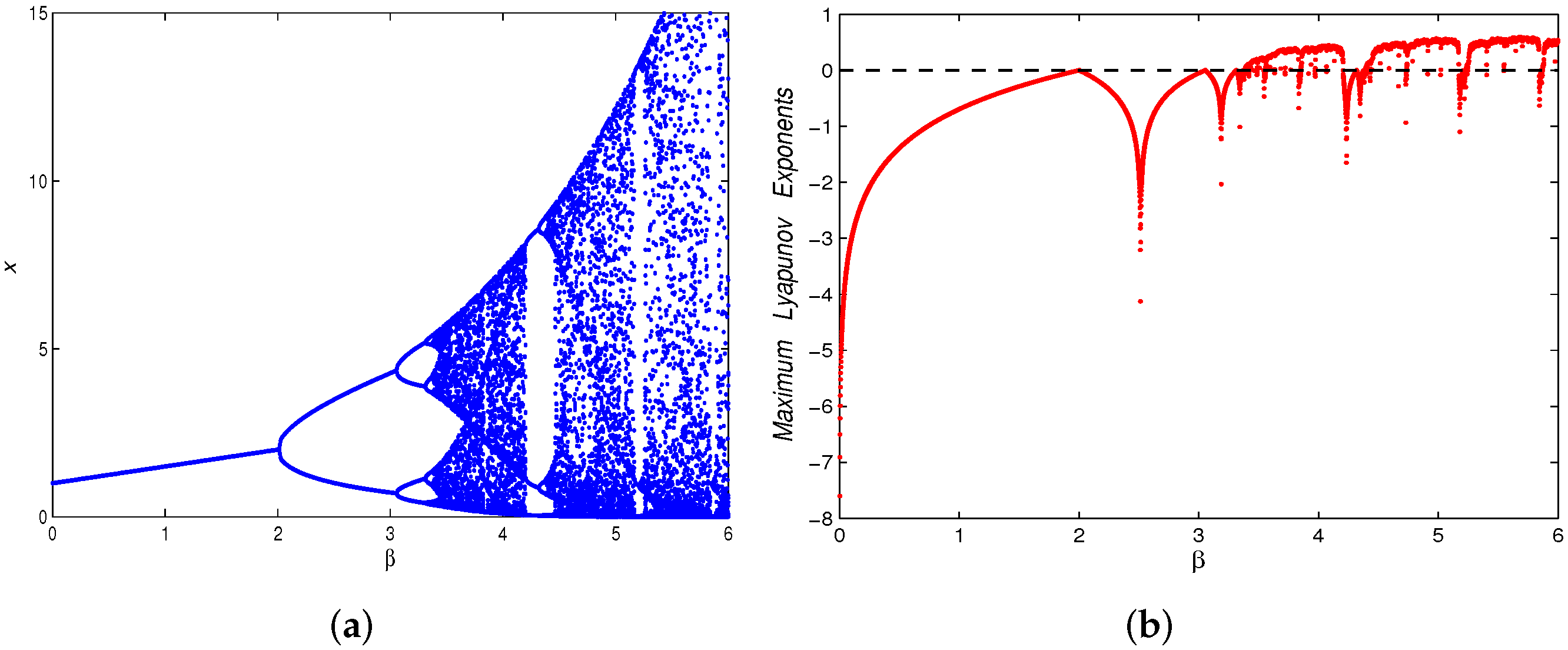
3.3.3. Bifurcation Analysis of Positive Fixed Point $E_{3j}^{*}(x_j^{*},y_j)(j=2,3)$

Theorem 12.

If $E_{3j}^{*}(x_j^{*},y_j)(j=2,3)$ exists, the map (5) has:

(a) 

A flip bifurcation for parameter $(\alpha ,\beta ,M,A)\in {\Omega }_{\mathit{E}{32}_{\mathit{FB}}}=\{(\alpha ,\beta ,M,A)\in {\mathbb{R}}^4:0<\alpha <2,$ $\beta ={\beta }_2^{*},M\ne M^{*},0<A<1\}$ at $E_{32}^{*}(x_2^{*},y_2)$.

(b) 

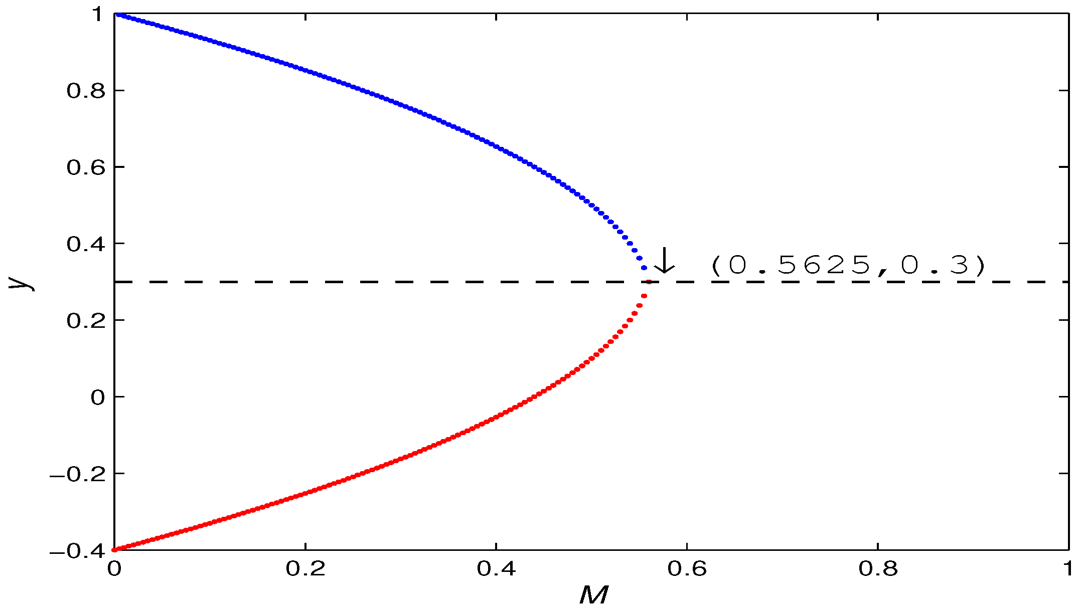
A fold bifurcation for parameter $(\alpha ,\beta ,M,A)\in {\Omega }_{\mathit{E}{33}_{\mathit{FOB}}}=\{(\alpha ,\beta ,M,A)\in {\mathbb{R}}^4:0<\alpha <2,$ $M=M^{*},0<A<1,\beta >0and\beta \ne {\beta }_3^{*}\}$ at $E_{33}^{*}(x_3^{*},y_3)$. In addition, with the increase of M, the number of positive fixed points of the map (5) has a 2-1-0 change. That is, when $M<M^{*}$, there are $E_{31}^{*}(x_1^{*},y_1)$ and $E_{32}^{*}(x_2^{*},y_2)$; when $M=M^{*}$, there is a unique positive fixed point $E_{33}^{*}(x_3^{*},y_3)$, and when $M>M^{*}$ the positive fixed point disappears.

Proof. 

$\left(a\right)$ From Theorem 8$\left(2\right)\left(iii\right)$, we can easily obtain that, when $(\alpha ,\beta ,M,A)\in {\Omega }_{\mathit{E}{32}_{\mathit{FB}}}=\{(\alpha ,\beta ,M,A)\in {\mathbb{R}}^4:0<\alpha <2,\beta ={\beta }_2^{*},0<A<1,M\ne M^{*}\}$, ${\lambda }_1=-1,|{\lambda }_2|=|1 + y_2(-1+\frac{M}{{(y_2+A)}^2})|<1$. Then, to obtain the flip bifurcation, we regard $\beta$ as the bifurcation parameter and shift the fixed point $E_{32}^{*}(x_2^{*},y_2)$ to $(0,0)$ through a transformation $u=x-x_2^{*},v=y-y_2$ and $\delta =\beta -{\beta }_2^{*}$; here, $|\delta \parallel \ll 1$ and is a sufficiently small new variable. We then have

$$\left(\begin{array}{c}{\displaystyle u}\\ {\displaystyle v}\end{array}\right)\to \left(\begin{array}{cc}{a}_{001}& {\mathit{a}}_{010}\\ 0& {\mathit{b}}_{010}\end{array}\right)\left(\begin{array}{c}{\displaystyle u}\\ {\displaystyle v}\end{array}\right)+\left(\begin{array}{c}{\displaystyle f_5(u,v,\delta )}\\ {\displaystyle f_6(u,v,\delta )}\end{array}\right);$$

(28)

here,

$$\begin{array}{cc}\hfill f_5(u,v,\delta )& =a_{210}{u}^{2}v+a_{201}{u}^2\delta +a_{120}u{v}^2+a_{102}u{\delta }^2+a_{021}{v}^2\delta +a_{012}v{\delta }^2+a_{110}uv\hfill \\ \hfill & + a_{300}{u}^3+a_{101}u\delta +a_{011}v\delta +a_{020}{v}^2+a_{111}uv\delta +a_{200}{u}^2+a_{003}{\delta }^3\hfill \\ \hfill & + a_{002}{\delta }^2+a_{030}{v}^3+O\left({(\left|u\right|+\left|v\right|+\left|\delta \right|)}^3\right)\hfill \\ \hfill f_6(u,v,\delta )& =b_{020}{v}^2+b_{030}{v}^3+O\left({(\left|u\right|+\left|v\right|+\left|\delta \right|)}^3\right),\hfill \end{array}$$

and

$$\begin{array}{cc}\hfill a_{100}& =1-x_2^{*},a_{001}=x_2^{*}{y}_2,a_{010}=x_2^{*}{\beta }_2^{*},\hfill \\ \hfill a_{210}& =\frac{{\beta }_2^{*}(x_2^{*}-2)}{2},a_{201}=\frac{y_2(x_2^{*}-2)}{2},a_{120}=-\frac{{{\beta }_2^{*}}^2(x_2^{*}-1)}{2},\hfill \\ \hfill a_{102}& =-\frac{y_2^2(x_2^{*}-1)}{2},a_{021}=\frac{x_2^{*}{\beta }_2^{*}({\beta }_2^{*}{y}_2+2)}{2},a_{012}=\frac{x_2^{*}{y}_2({\beta }_2^{*}{y}_2+2)}{2},\hfill \\ \hfill a_{110}& =-{\beta }_2^{*}(x_2^{*}-1),a_{300}=-\frac{x_2^{*}}{6}+\frac{1}{2},a_{101}=-y_2(x_2^{*}-1),\hfill \\ \hfill a_{011}& =x_2^{*}({\beta }_2^{*}{y}_2+1),a_{020}=\frac{x_2^{*}{{\beta }_2^{*}}^2}{2},a_{111}=(1-x_2^{*})(1+{\beta }_2^{*}{y}_2),\hfill \\ \hfill a_{200}& =\frac{x_2^{*}}{2}-1,a_{003}=\frac{x_2^{*}{y}_2^3}{6},a_{002}=\frac{x_2^{*}{y}_2^2}{2},a_{030}=\frac{{x_2^{*}}^3}{6},\hfill \\ \hfill b_{010}& =-\frac{1}{{(A+y_2)}^2}(A^2{y}_2+2A{y}_2^2+y_2^3-A^2-2A{y}_2-M{y}_2-y_2^2),\hfill \\ \hfill b_{020}& =\frac{1}{2{(A+y_2)}^4}(A^4{y}_2+4A^3{y}_2^2+6A^2{y}_2^3+4A{y}_2^4+y_2^5-2A^4\hfill \\ \hfill & - 8A^3{y}_2-2A^{2}M{y}_2-12A^2{y}_2^2-4AM{y}_2^2-8A{y}_2^3-2M{y}_2^3\hfill \\ \hfill & - 2y_2^4+2A^{2}M+2AM{y}_2+M^2{y}_2),\hfill \\ \hfill b_{030}& =\frac{1}{6{(A+y_2)}^6}(A^6{y}_2+6A^5{y}_2^2+15A^4{y}_2^3+20A^3{y}_2^4+15A^2{y}_2^5+6A{y}_2^6\hfill \\ \hfill & - 18A^5{y}_2-3A^{4}M{y}_2-45A^4{y}_2^2-12A^{3}M{y}_2^2-60A^3{y}_2^3-18A^{2}M{y}_2^3\hfill \\ \hfill & - 12AM{y}_2^4-18A{y}_2^5+y_2^7-3A^6-3M{y}_2^5-3y_2^6+6A^{4}M+18A^{3}M{y}_2\hfill \\ \hfill & + 3A^2{M}^2{y}_2+18A^{2}M{y}_2^2+6A{M}^2{y}_2^2+6AM{y}_2^3+3M^2{y}_2^3+6A^{3}M\hfill \\ \hfill & - 45A^2{y}_2^4-3A^2{M}^2+12A^{2}M{y}_2+6AM{y}_2^2-M^3{y}_2+3M^2{y}_2^2).\hfill \end{array}$$

The linearization matrix for the map (28) is

$$J\left(E_{32}^{*}\right)=\left(\begin{array}{cc}{\mathit{a}}_{100}& {\mathit{a}}_{010}\\ 0& {\mathit{b}}_{010}\end{array}\right).$$

Find an invertible matrix T, for instance

$$T=\left(\begin{array}{cc}{\mathit{a}}_{010}& {\mathit{a}}_{010}\\ -1-{\mathit{a}}_{100}& {\lambda }_2-{\mathit{a}}_{100}\end{array}\right)$$

and make the transformation:

$$\left(\begin{array}{c}u\\ v\end{array}\right)=T\left(\begin{array}{c}X\\ Y\end{array}\right),$$

(29)

the map (18) yields

$$\left(\begin{array}{c}{\displaystyle X}\\ {\displaystyle Y}\end{array}\right)\to \left(\begin{array}{cc}-1& 0\\ 0& {\lambda }_2\end{array}\right)\left(\begin{array}{c}{\displaystyle X}\\ {\displaystyle Y}\end{array}\right)+\left(\begin{array}{c}{\displaystyle G_5(X,Y,\delta )}\\ {\displaystyle G_6(X,Y,\delta )}\end{array}\right),$$

(30)

where

$$\begin{array}{cc}\hfill G_5(X,Y,\delta )& =K_{300}{X}^3+K_{210}{X}^{2}Y+K_{201}{X}^2\delta +K_{200}{X}^2+K_{120}X{Y}^2+K_{111}XY\delta \hfill \\ \hfill & + K_{110}XY+K_{102}X{\delta }^2+K_{101}X\delta +K_{030}{Y}^3+K_{020}{Y}^2+K_{021}{Y}^2\delta \hfill \\ \hfill & + K_{012}Y{\delta }^2+K_{011}Y\delta +K_{003}{\delta }^3+K_{002}{\delta }^2+O\left({(\left|X\right|+\left|Y\right|+\left|\delta \right|)}^3\right),\hfill \\ \hfill G_6(X,Y,\delta )& =C_{300}{X}^3+C_{210}{X}^{2}Y+C_{200}{X}^2+C_{120}X{Y}^2+C_{110}XY+C_3{Y}^3+C_2{Y}^2\hfill \\ \hfill & + O\left({(\left|X\right|+\left|Y\right|+\left|\delta \right|)}^3\right),\hfill \end{array}$$

where

$$\begin{array}{cc}\hfill K_{300}& =a_{030}{\Gamma }^3+a_{120}{a}_{010}{\Gamma }^2+a_{210}{a}_{010}^2\Gamma +a_{300}{a}_{010}^3,\hfill \\ \hfill K_{210}& =3a_{030}\mathsf{\Theta }{\Gamma }^2+a_{120}{a}_{010}{\Gamma }^2+2a_{120}{a}_{010}\Gamma \mathsf{\Theta }+3a_{210}{a}_{010}^2\Gamma +3a_{300}{a}_{010}^3,\hfill \\ \hfill K_{201}& =a_{021}{\Gamma }^2+a_{111}{a}_{010}\Gamma +a_{201}{a}_{010}^2,\hfill \\ \hfill K_{200}& =a_{020}{\Gamma }^2+a_{110}{a}_{010}\Gamma +a_{200}{a}_{010}^2,\hfill \\ \hfill K_{120}& =3a_{030}\Gamma {\mathsf{\Theta }}^2+2a_{120}{a}_{010}\Gamma \mathsf{\Theta }+a_{210}{a}_{010}^2\Gamma +a_{120}{a}_{010}{\mathsf{\Theta }}^2+2a_{210}{a}_{010}^2\mathsf{\Theta }+3a_{300}{a}_{010}^3,\hfill \\ \hfill K_{111}& =2a_{021}\mathsf{\Theta }\Gamma +a_{111}{a}_{010}\Gamma +a_{111}{a}_{010}\mathsf{\Theta }+2a_{201}{a}_{010}^2,\hfill \\ \hfill K_{110}& =2a_{020}\mathsf{\Theta }\Gamma +a_{110}{a}_{010}\Gamma +a_{110}{a}_{010}\mathsf{\Theta }+2a_{200}{a}_{010}^2,\hfill \\ \hfill K_{102}& =a_{012}\Gamma +a_{102}{a}_{010},K_{101}=a_{011}\Gamma +a_{010}{a}_{101},\hfill \\ \hfill K_{030}& =a_{030}{\mathsf{\Theta }}^3+a_{120}{a}_{010}{\mathsf{\Theta }}^2+a_{210}{a}_{010}^2\mathsf{\Theta }+a_{300}{a}_{010}^3,\hfill \\ \hfill K_{021}& =a_{021}{\mathsf{\Theta }}^2+a_{111}{a}_{010}\mathsf{\Theta }+a_{201}{a}_{010}^2,\hfill \\ \hfill K_{020}& =a_{020}\mathsf{\Theta }+a_{110}{a}_{010}\mathsf{\Theta }+a_{200}{a}_{010}^2,\hfill \\ \hfill K_{012}& =\mathsf{\Theta }{a}_{012}+a_{010}{a}_{102},\hfill \\ \hfill K_{011}& =a_{011}\mathsf{\Theta }+a_{010}{a}_{101},K_{003}=a_{003},\hfill \\ \hfill K_{002}& =a_{002},C_{300}=b_{030}{\Gamma }^3,\hfill \\ \hfill C_{210}& =3b_{030}\mathsf{\Theta }{\Gamma }^2,C_{200}=b_{020}{\Gamma }^2,C_{120}=3b_{030}{\mathsf{\Theta }}^2\Gamma ,\hfill \\ \hfill C_{110}& =2b_{020}\mathsf{\Theta }\Gamma ,C_{003}=b_{030}{\mathsf{\Theta }}^3,C_{002}=b_{020}{\mathsf{\Theta }}^2,\hfill \\ \hfill \Gamma & =(-1-a_{100}),\mathsf{\Theta }={\lambda }_2-a_{100}.\hfill \end{array}$$

According to the center manifold theory, a one-parameter simplified system of equations restricted to the manifold determines the stability of $(X,Y)=(0,0)$ in the neighborhood of $\delta =0$, given by

$$W^c(0,0,0)=\left\{(X,Y,\delta )\in {\mathbb{R}}^3:Y=g(X,\delta ),g(0,0)=0,Dg(0,0)=0\right\}$$

with X and $\delta$ sufficiently small. Moreover, let

$$g(X,\delta )=g_1\delta +g_2{\mathit{X}}^2+g_3\mathit{X}\delta +g_4{\delta }^2+O\left(\right(\left|X\right|+{\left|\delta \right|)}^3);$$

(31)

thus,

$$N\left(g(X,\delta )\right)=g(-X+G_5(X,g(X,\delta ),\delta ),\delta )-{\lambda }_{2}g(X,\delta )-G_6(X,g(X,\delta ),\delta )=0.$$

(32)

From (31) and (32), we obtain

$$\begin{array}{cc}\hfill {\mathit{g}}_1& =0,{\mathit{g}}_2=\frac{C_{200}}{1-{\lambda }_2},{\mathit{g}}_3=\frac{C_{110}{g}_1}{1+{\lambda }_2},{\mathit{g}}_4=\frac{C_{002}{g}_1^2}{1-{\lambda }_2}.\hfill \end{array}$$

Hence, the map restricted to the center manifold becomes

$$\begin{array}{cc}\hfill F_3:X& \to -X+{\mathit{s}}_0\delta +s_1{X}^2+s_{2}X\delta +s_3{\delta }^2+s_4{X}^2\delta +s_{5}X{\delta }^2\hfill \\ \hfill & + s_6{X}^3+s_7{\delta }^3+O\left({(\left|X\right|+\left|\delta \right|)}^3\right).\hfill \end{array}$$

where

$$\begin{array}{cc}\hfill s_0& =0,s_1=K_{200},s_2=K_{101},s_3=K_{002},s_4=K_{201}-\frac{C_{200}{K}_{011}}{{\lambda }_2-1},\hfill \\ \hfill {\mathrm{s}}_5& =K_{102},s_6=K_{300}-\frac{K_{110}{C}_{200}}{{\lambda }_2-1},{\mathrm{s}}_7=K_{003}.\hfill \end{array}$$

We give the following two transversal conditions in [44]:

$$\begin{array}{cc}\hfill {\alpha }_1& =\left[\frac{{\partial }^2{F}_3}{\partial X\partial \delta }+\frac{1}{2}\frac{\partial F_3}{\partial \delta }\frac{{\partial }^2{F}_3}{\partial X^2}\right](0,0)=s_2+s_0{s}_1\ne 0,\hfill \\ \hfill {\alpha }_2& =\left[\frac{1}{6}\left(\frac{{\partial }^3{F}_3}{\partial X^3}\right)+{\left(\frac{1}{2}\frac{{\partial }^2{F}_3}{\partial X^2}\right)}^2\right](0,0)=s_6+s_1^2\ne 0.\hfill \end{array}$$

Therefore, a flip bifurcation occurs when $(\alpha ,\beta ,M,A)\in {\Omega }_{\mathit{E}{32}_{\mathit{FB}}}$ at the fixed point $E_{32}^{*}(x_2^{*},y_2)$.

$\left(b\right)$ From Theorem 8(3), it is easy to obtain that, when $(\alpha ,\beta ,M,A)\in {\Omega }_{\mathit{E}{33}_{\mathit{FOB}}}=\{(\alpha ,\beta ,M,A)\in {\mathbb{R}}^4:0<\alpha <2,M=M^{*},0<A<1,\beta >0and\beta \ne {\beta }_3^{*}\}$, $|{\lambda }_1| =|1 - x_3^{*}|\ne 1,{\lambda }_2=1$. Now, we select M as the bifurcation parameter. Take $\zeta =M-M^{*}$, $\left|\zeta \right|\ll 1$, and it is a new variable. We transform the fixed point $E_{33}^{*}(x_3^{*},\frac{1-A}{2})$ of the map (5) to $(0,0)$ with $u=x-x_3^{*},v=y-\frac{1-A}{2}$, and then, the map (5) becomes

$$\left(\begin{array}{c}{\displaystyle u}\\ {\displaystyle \zeta }\\ {\displaystyle v}\end{array}\right)\to \left(\begin{array}{ccc}1-x_3^{*}& 0& \beta x_3^{*}\\ 0& 1& 0\\ 0& \frac{A-1}{1+A}& 1\end{array}\right)\left(\begin{array}{c}{\displaystyle u}\\ {\displaystyle \zeta }\\ {\displaystyle v}\end{array}\right)+\left(\begin{array}{c}{\displaystyle f_7(u,v,\zeta )}\\ {\displaystyle 0}\\ {\displaystyle f_8(u,v,\zeta )}\end{array}\right),$$

(33)

where

$$\begin{array}{cc}\hfill f_7(u,v,\zeta )& =\left(\frac{{\mathit{x}}_3^{*}}{2}-1\right)u^2+\frac{{\beta }^2{\mathit{x}}_3^{*}}{2}{v}^2-\beta ({\mathit{x}}_3^{*}-1)uv+\left(\frac{1}{2}-\frac{{\mathit{x}}_3^{*}}{6}\right)u^3+\frac{{\beta }^3{\mathit{x}}_3^{*}}{6}{v}^3\hfill \\ \hfill & + \frac{\beta ({\mathit{x}}_3^{*}-2)}{2}{u}^{2}v-\frac{{\beta }^2({\mathit{x}}_3^{*}-1)}{2}u{v}^2+O\left({(\left|u\right|+\left|v\right|+\left|\zeta \right|)}^3\right),\hfill \\ \hfill f_8(u,v,\zeta )& =\frac{A-1}{1+A}{v}^2-\frac{4A}{{(1+A)}^2}v\zeta -\frac{A-1}{{(1+A)}^2}{\zeta }^2-\frac{4A}{{(1+A)}^2}{v}^3\hfill \\ \hfill & - \frac{2(A^2-4A-1)}{{(1+A)}^3}{v}^2\zeta +\frac{2(3A-1)}{{(1+A)}^3}v{\zeta }^2+\frac{2(A-1)}{3{(1+A)}^3}{\zeta }^3\hfill \\ \hfill & + O\left({(\left|u\right|+\left|v\right|+\left|\zeta \right|)}^3\right).\hfill \end{array}$$

The coefficient matrix is given by

$$J\left(E_{33}^{*}\right)=\left(\begin{array}{ccc}1-x_3^{*}& 0& \beta x_3^{*}\\ 0& 1& 0\\ 0& \frac{A-1}{1+A}& 1\end{array}\right).$$

Convertthe matrix $J\left(E_{33}^{*}\right)$ in (33) into the normal form with matrix translation as follows:

$$\left(\begin{array}{c}u\\ \zeta \\ v\end{array}\right)=T\left(\begin{array}{c}X\\ \eta \\ Y\end{array}\right),$$

(34)

where

$$T=\left(\begin{array}{ccc}\beta & -\frac{\beta }{x_3^{*}}& 1\\ 0& \frac{1+A}{A-1}& 0\\ 1& 0& 0\end{array}\right)$$

is an invertible matrix. From (33) and (34), we have

$$\left(\begin{array}{c}{\displaystyle X}\\ {\displaystyle \eta }\\ {\displaystyle Y}\end{array}\right)\to \left(\begin{array}{ccc}1& 1& 0\\ 0& 1& 0\\ 0& 0& 1-x_3^{*}\end{array}\right)\left(\begin{array}{c}{\displaystyle X}\\ {\displaystyle \eta }\\ {\displaystyle Y}\end{array}\right)+\left(\begin{array}{c}{\displaystyle G_7(X,Y,\eta )}\\ {\displaystyle 0}\\ {\displaystyle G_8(X,Y,\eta )}\end{array}\right),$$

(35)

where

$$\begin{array}{cc}\hfill G_7(X,Y,\eta )& =p_{101}X\eta +p_{200}{X}^2+p_{102}X{\eta }^2+p_{300}{X}^3+p_{201}{X}^2\eta +p_{002}{\eta }^2\hfill \\ \hfill & + p_{003}{\eta }^3+O\left({(\left|X\right|+\left|Y\right|+\left|\eta \right|)}^3\right),\hfill \\ \hfill G_8(X,Y,\eta )& =m_{300}{X}^3+m_{201}{X}^2\eta +m_{200}{X}^2+m_{102}X{\eta }^2+m_{101}X\eta \hfill \\ \hfill & + m_{020}{Y}^2+m_{021}{Y}^2\eta +m_{011}Y\eta +m_{012}Y{\eta }^2+m_{002}{\eta }^2\hfill \\ \hfill & + m_{111}XY\eta +m_{120}X{Y}^2+m_{003}{\eta }^3+O\left(\right(\left|X\right|+\left|Y\right|+{\left|\eta \right|)}^3),\hfill \end{array}$$

and

$$\begin{array}{cc}\hfill p_{101}& =-\frac{4A}{(1+A)(A-1)},p_{200}=\frac{A-1}{1+A},\hfill \\ \hfill p_{102}& =-\frac{2(-1+3A)}{(1+A){(A-1)}^2},p_{300}=-\frac{4A}{{(1+A)}^2},\hfill \\ \hfill p_{201}& =-\frac{2(A^2-4A-1)}{{(1+A)}^2(A-1)},p_{002}=\frac{1}{A-1},\hfill \\ \hfill p_{003}& =\frac{2}{3{(A-1)}^2},m_{300}=\frac{4\beta A}{{(1+A)}^2},\hfill \\ \hfill m_{201}& =\frac{2\beta (A^2-4A-1)}{{(1+A)}^2(A-1)},m_{200}=-\frac{\beta (A-1)}{1+A},\hfill \\ \hfill m_{102}& =\left(\frac{{\beta }^3}{2x_3^{*2}}+\frac{(2-6A)\beta }{(1+A){(A-1)}^2}\right),m_{101}=\left(\frac{{\beta }^2}{x_3^{*}}+\frac{4\beta A}{(1+A)(A-1)}\right),\hfill \\ \hfill m_{020}& =\left(\frac{(1-A)\beta }{4}+\frac{\alpha }{2}-1\right),m_{021}=\frac{\beta \left(\right(A-1)\beta -2\alpha +6)}{(2A-2)\beta -4\alpha },\hfill \\ \hfill m_{011}& =-\frac{\left(\right(A-1)\beta -2\alpha +4)\beta }{(A-1)\beta -2\alpha },m_{012}=\frac{{\beta }^2((A-1)\beta -2\alpha +6)}{{((A-1)\beta -2\alpha )}^2},\hfill \\ \hfill m_{002}& =-\frac{2((A-1)(\alpha +2)\beta -2{\alpha }^2)\beta }{(A-1){((A-1)\beta -2\alpha )}^2},m_{111}=-\left(\beta +\frac{{\beta }^2}{x_3^{*}}\right),m_{120}=\frac{\beta }{2},\hfill \\ \hfill m_{003}& =\frac{8((\alpha +\frac{3}{2}){(A-1)}^2{\beta }^2-3{\alpha }^2(A-1)\beta +2{\alpha }^3)\beta }{3{(A-1)}^2{((A-1)\beta -2\alpha )}^3}.\hfill \end{array}$$

By implementing the center manifold theorem, the stability of the map (35) at $(X,Y)=(0,0)$ in a neighborhood of $\eta =0$ can be approximated as follows:

$$W^c(0,0,0)=\left\{(X,Y,\eta )\in {\mathbb{R}}^3:Y=g(X,\eta ),g(0,0)=0,Dg(0,0)=0\right\}$$

with X and $\eta$ small. Then, assume

$$g(X,\eta )=g_1{X}^2+g_{2}X\eta +g_3{\eta }^2+O\left({(\left|X\right|+\left|\eta \right|)}^3\right),$$

(36)

and $g(X,\eta )$ have the following equation

$$N\left(g(X,\eta )\right)=g(X+\eta +G_7(X,g(X,\eta ),\eta ),\eta )-(1-x_3^{*})g(X,\eta )-G_8(X,g(X,\eta ),\eta )=0.$$

(37)

Substituting (36) into (37) and comparing the coefficients of $X^2,X\eta$, and ${\eta }^2$ in (37), we obtain

$$\begin{array}{cc}\hfill g_1& =\frac{(1-A)\beta }{(A+1)x_3^{*}},\hfill \\ \hfill g_2& =\frac{({(A-1)}^2\beta -4A\alpha )\beta }{(A^2-1)x_3^{*2}}+\frac{2g_1}{x_3^{*}},\hfill \\ \hfill g_3& =\frac{\beta ((\alpha +2)(1-A)\beta +{\alpha }^2)}{2(A-1)x_3^{*3}}-\frac{g_1+g_2}{x_3^{*}}.\hfill \end{array}$$

Thus, the restricted map to the center manifold $W^c(0,0,0)$ is given as

$$\begin{array}{cc}\hfill F_4:X& \to X+\eta +\frac{A-1}{1+A}{X}^2-\frac{4A}{(1+A)(A-1)}X\eta -\frac{1}{A-1}{\eta }^2\hfill \\ \hfill & - \frac{4A}{{(1+A)}^2}{X}^3-\frac{2(A^2-4A-1)}{{(1+A)}^2(A-1)}{X}^2\eta +\frac{2}{3{(A-1)}^2}{\eta }^3\hfill \\ \hfill & + \frac{2(3A-1)}{(1+A){(A-1)}^2}X{\eta }^2+O\left({(\left|X\right|+\left|\eta \right|)}^3\right).\hfill \end{array}$$

We can simply calculate

$$\begin{array}{cc}\hfill & F_4(0,0)=0,\frac{\partial F_4}{\partial X}(0,0)=1,\frac{\partial F_4}{\partial \eta }(0,0)=1,\hfill \\ \hfill & \frac{{\partial }^2{F}_4}{\partial X^2}(0,0)=\frac{2(A-1)}{1+A}\ne 0,\frac{{\partial }^2{F}_4}{\partial X\partial \eta }(0,0)=-\frac{4A}{(1+A)(A-1)}\ne 0,\hfill \end{array}$$

which leads to a fold bifurcation when $(\alpha ,\beta ,M,A)\in {\Omega }_{\mathit{E}{33}_{\mathit{FOB}}}$ at the $E_{33}^{*}(x_3^{*},\frac{1-A}{2})$. □

3.4. Chaos Control

From Theorem 12(a), it can be seen that a flip bifurcation of the map (5) is shown at the coexistence fixed point $E_{32}^{*}=(x_2^{*},y_2)$. This will cause chaos in the system, so we use a hybrid chaos-control method in [46], which is a combination of parameter perturbation and feedback control, to delay or get rid of chaos. First, the control system corresponding to the map (5) is given by

$$\left(\begin{array}{c}{\displaystyle x}\\ {\displaystyle y}\end{array}\right)\to \left(\begin{array}{c}{\displaystyle \rho xexp(\alpha -x+\beta y)+(1-\rho )x)}\\ {\displaystyle \rho yexp(1-y-\frac{M}{y+A})+(1-\rho )y)}\end{array}\right).$$

(38)

where $0<\rho <1$ and $\rho$ is an external control parameter. Moreover, the calculation shows that System (38) and the map (5) have the same fixed points. The linearized Jacobian matrix of the map (38) at fixed point $E_{32}^{*}=(x_2^{*},y_2)$ is

$$J\left(E_{32}^{*}\right)=\left(\begin{array}{cc}1-\rho {\mathit{x}}_2^{*}& \rho {\mathit{x}}_2^{*}\beta \\ 0& 1+\rho y_2\left(-1+\frac{M}{{(y_2+A)}^2}\right)\end{array}\right).$$

Obviously, the two eigenvalues of the Jacobian matrix $J\left(E_{32}^{*}\right)$ are ${\lambda }_1=1-\rho {\mathit{x}}_2^{*}<1$ and ${\lambda }_2=1+\rho y_2\left(-1+\frac{M}{{(y_2+A)}^2}\right)$. According to the previous analysis, $J_2<1$, then $-1+\frac{M}{{(y_2+A)}^2}<0$. We have ${\lambda }_2=1+\rho y_2\left(-1+\frac{M}{{(y_2+A)}^2}\right)<1$. Therefore, with the help of Definition 1(1), the controlled system (38) has the following statement.

Theorem 13.

If and only if

$$\rho {\mathit{x}}_2^{*}<2and\rho {\mathit{y}}_2\left(1-\frac{M}{{({\mathit{y}}_2+A)}^2}\right)<2$$

holds, the coexistence fixed point $E_{32}^{*}(x_2^{*},y_2)$ of the map (38) is locally asymptotically stable.

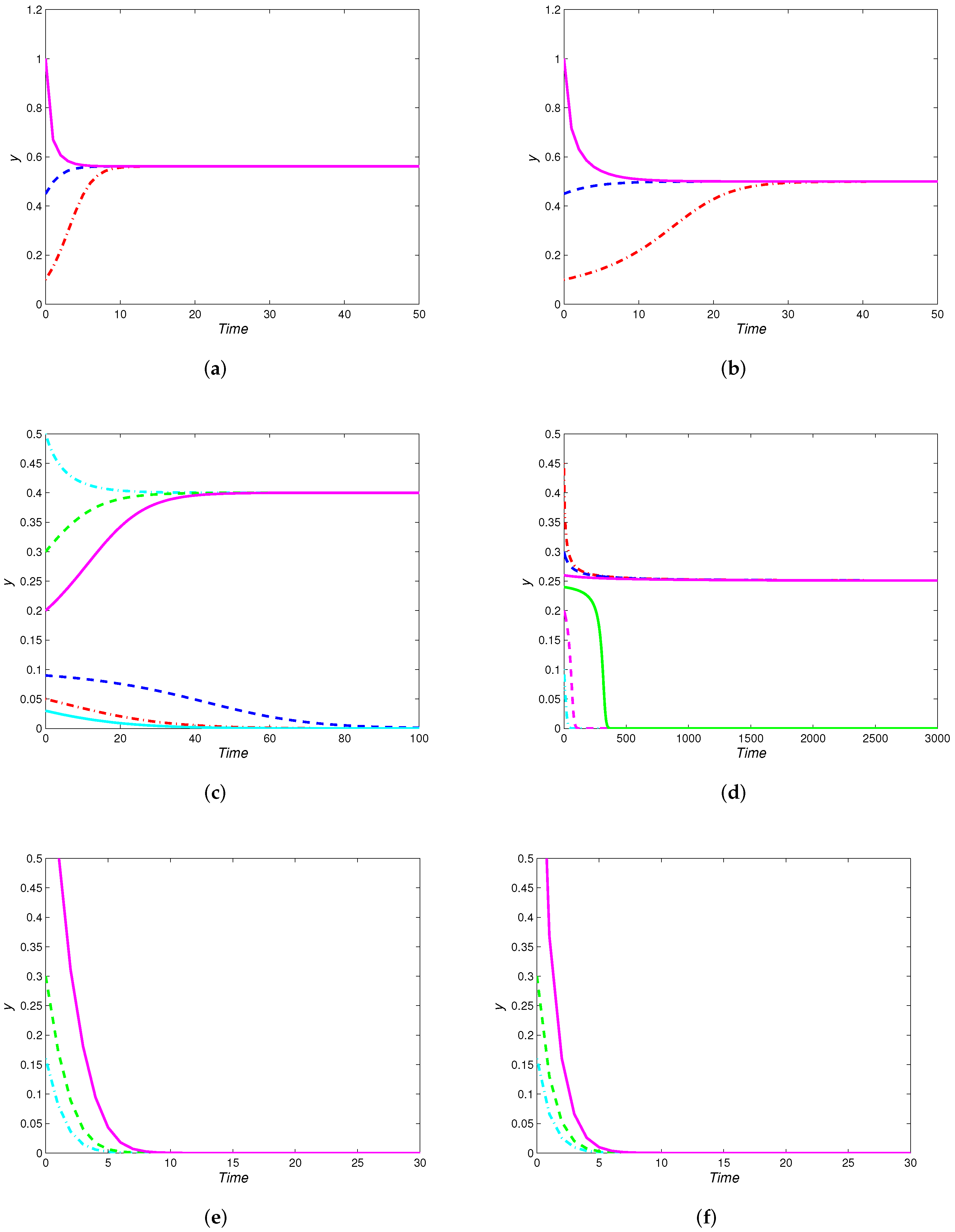
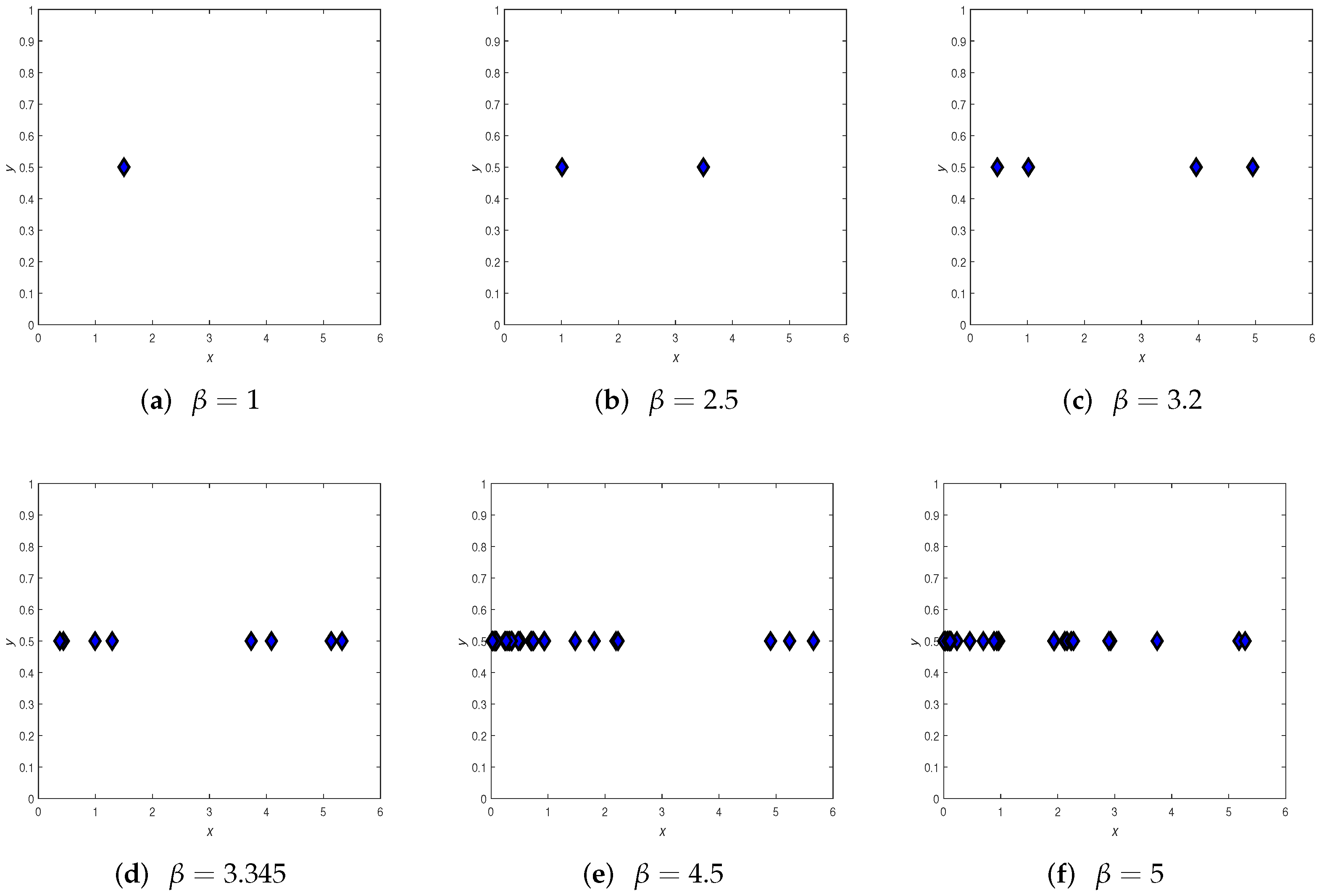
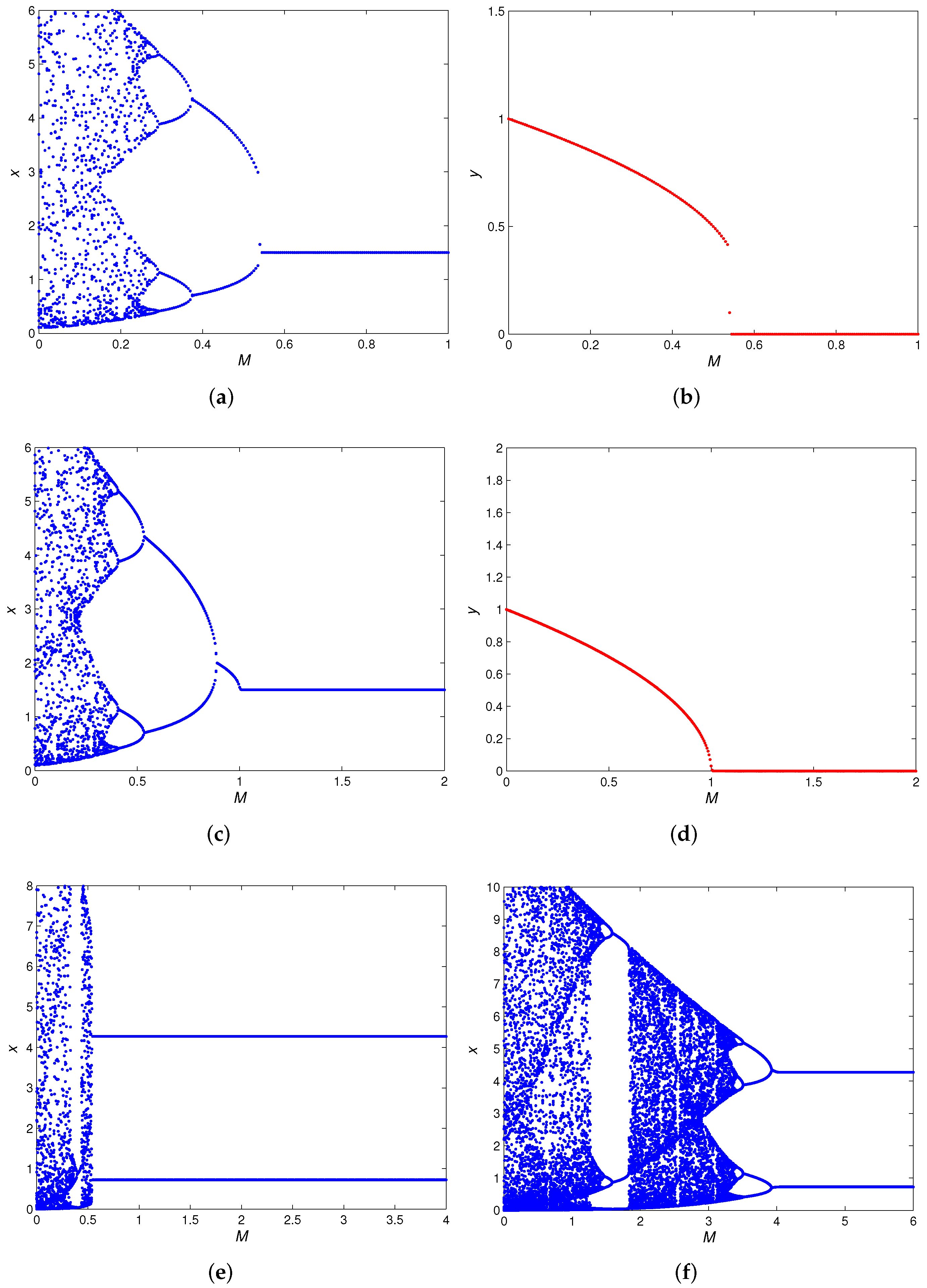
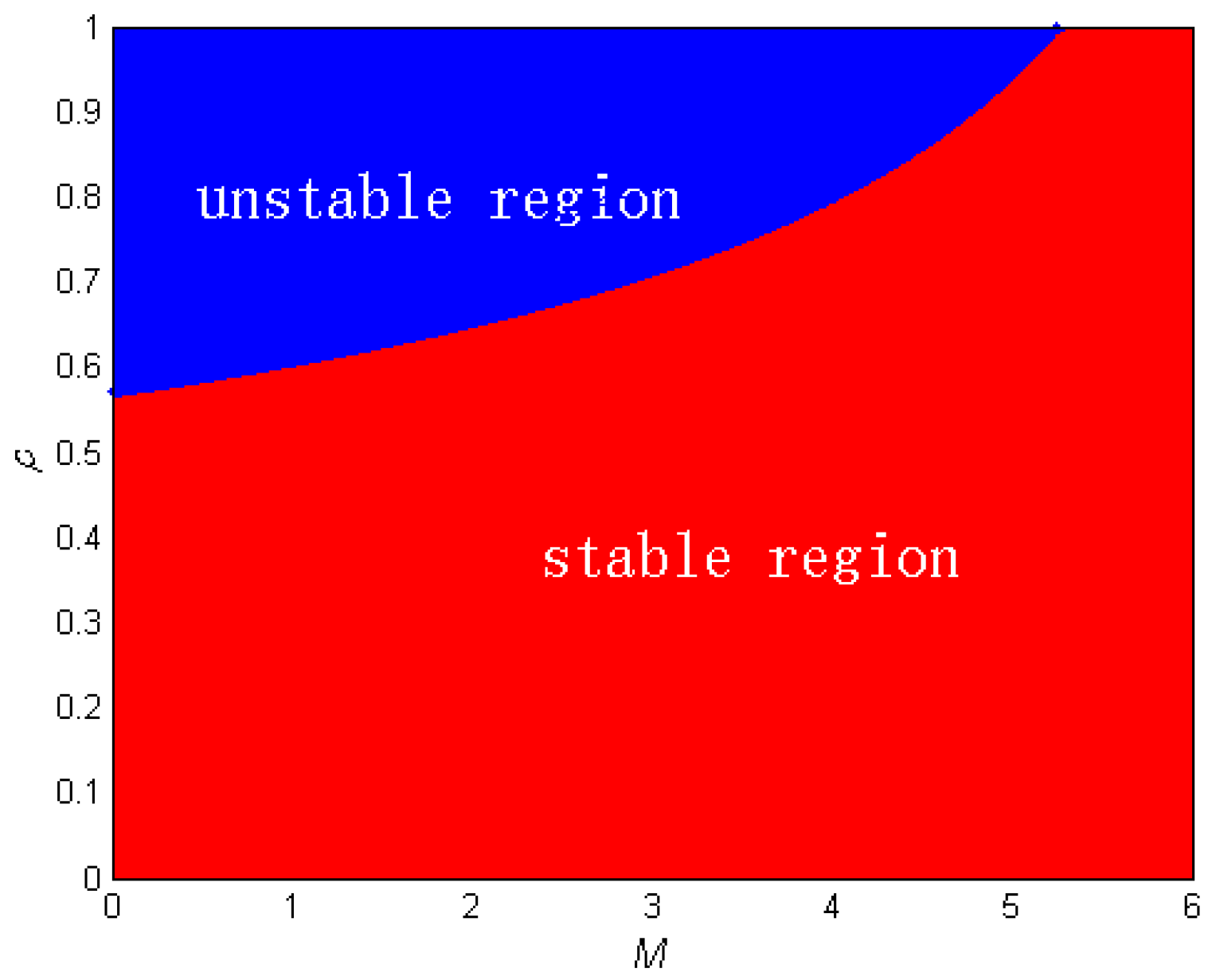
4. Numerical Simulations

In this section, the analysis results obtained above are further studied through numerical simulations.

Case (1): Select different parameters of the map (6), in Table 3, to observe the solution curve in Figure 6.

Table 3. Parameter table.

Parameter	Positive Fixed Point	Initial Value
$M=2,A=4$	$y_2=0.5616$	$y\left(0\right)=0.1,0.5,1$
$M=A=0.5$	$y_2=0.5$	$y\left(0\right)=0.1,0.5,1$
$M=0.54,A=0.5$	$y_1=0.1,y_2=0.4$	$y\left(0\right)=0.09,0.05,0.02,0.2,0.3.0.5$
$M=0.5625,A=0.5$	$y_3=0.25$	$y\left(0\right)=0.09,0.2,0.24,0.26,0.3.0.45$
$M=1,A=0.5$	no	$y\left(0\right)=0.15,0.3,1$
$M=2,A=1$	no	$y\left(0\right)=0.15,0.3,1$

Figure 6. (a) With $M=2,A=4$, and the initial value as $y\left(0\right)=0.1,0.5,1$, the map (6) has positive fixed points $y_2=0.5616$; (b) with $M=A=0.5$ and the initial value as $y\left(0\right)=0.1,0.5,1$, the map (6) has positive fixed points $y_2=0.5$; (c) with $M=0.54,A=0.5$, and the initial value as $y\left(0\right)=0.09,0.05,0.02,0.2,0.3.0.5$, the map (6) has two positive fixed points $y_1=0.1,y_2=0.4$; (d) with $M=0.5625,A=0.5$, and the initial value as $y\left(0\right)=0.09,0.05,0.02,0.2,0.3.0.5$, the map (6) has positive fixed points $y_3=0.25$; (e) with $M=1,A=0.5$, and the initial value as $y\left(0\right)=0.15,0.3,1$, the map (6) has no positive fixed point; (f) with $M=1,A=1$, and the initial value as $y\left(0\right)=0.15,0.3,1$, the map (6) has no positive fixed point.

Case (2): Set parameters $\alpha =\beta =1,M=2,A=4$ and initial values as $\left(x\right(0),y(0\left)\right)=\left(\right(1.5,0.3),(1.2,0.6),(0.8,0.2\left)\right)$ in the map (5). There is a positive fixed point $E_{32}^{*}(1.5616,0.5616)$ and global asymptotic stability by Theorem 9. Figure 7 shows the result.

Figure 7. Stability of the fixed point $E_{32}^{*}$ of the map (5) with $\alpha =\beta =1,M=2,A=4$, and the initial values as $\left(x\right(0),y(0\left)\right)=\left(\right(1.5,0.3),(1.2,0.6),(0.8,0.2\left)\right)$.

Case (3): Set parameters $\alpha =3,\beta =1,A=0.15$ in the map (5). We find that the two eigenvalues of the Jacobian matrix $J\left(E_1\right)$ at the boundary fixed point $E_1(3,0)$ are ${\lambda }_1=-2,$ ${\lambda }_2=1$. Therefore, by Theorem 6, the fixed point $E_1(3,0)$ is non-hyperbolic. According to Theorem 11(i) of the bifurcation analysis, the map (5) has transcritical bifurcation at $E_1$.

Figure 8 is a diagram of the transcritical bifurcation on the $M-y$ plane in the local range of the fixed point $E_1(3,0)$ when $M\in [0,0.331]$, and the other parameters are given in Case (3). From Figure 8, it can be found that, when $M<0.15$, $E_1(3,0)$ is unstable, but when $M>0.15$, there is a stable fixed point $E_1(3,0)$ and an unstable fixed point $E_{31}^{*}(3.425-\frac{\sqrt{1.3225-4M}}{2},0.425-\frac{\sqrt{1.3225-4M}}{2})$.

Figure 8. Transcritical bifurcation diagrams in the $M-y$ plane with $\alpha =3,\beta =1,A=0.15$.

Case (4): Further, based on Case (3), we change the parameter A and let $A=1$. At this time, by Theorem 11(ii), the map (5) generates a pitchfork bifurcation at $E_1(3,0)$. Namely, it is a pitchfork bifurcation point.

Figure 9 is a diagram of the pitchfork bifurcation on the $M-y$ plane in the local area of the fixed point $E_1$. Select the initial value of $x_0=0.5,y_0=0.3,M\in [0,1.5]$, $\alpha =3,$ and $\beta =1$. It can be seen from Figure 9 that the fixed point $E_1$ is unstable, when $M<1$; the stable fixed point $E_1(3,0)$ appears when $M>1$. Additionally, there are two stable fixed points $E_{31}^{*}=(3-\sqrt{1-M},-\sqrt{1-M})$ and $E_{32}^{*}=(3+\sqrt{1-M},\sqrt{1-M})$ when $M<1$; $E_{31}^{*}=(3-\sqrt{1-M},-\sqrt{1-M})$ and $E_{32}^{*}=(3+\sqrt{1-M},\sqrt{1-M})$ coincide to form the double-root $E_{33}^{*}(3,0)$ when $M=1$; $E_{33}^{*}$ disappears when $M>1$.

Figure 9. Pitchfork bifurcation diagrams in the $M-y$ plane with $\alpha =3,\beta =1,A=1$.

Case (5): Set the parameters $\alpha =1,M=0.4,A=0.3$ in the map (5). When $\beta =2$, the corresponding eigenvalues of the matrix $J\left(E_{32}^{*}\right)$ are ${\lambda }_1=-1,{\lambda }_2=0.8125$, respectively. From Theorem 8(2)(iii), $E_{32}^{*}(2,0.5)$ is non-hyperbolic. Further, from Theorem 12(a), the map (5) has a flip bifurcation at $E_{32}^{*}$.

Figure 10a describes the diagram of the flip bifurcation on the $\beta -x$ plane at the initial value $x_0=0.5,y_0=0.3$, $\beta \in [0,6]$, and the other parameters are shown in Case (5). From Figure 10a, the coexistence equilibria $E_{32}^{*}$ are stable when $\beta <2$, and when $\beta =2$, the map (5) is unstable, resulting in a stable two-period solution; when $\beta >3.065$, it will further generate four-dimensional solutions and constantly flip to generate chaotic sets.

Figure 10. (a) Flip bifurcation diagrams on the $\beta -x$ plane with $\alpha =1,M=0.4,A=0.3$; (b) maximum Lyapunov exponents corresponding to (a).

Figure 10b shows the maximum Lyapunov exponents of Figure 10a, and $\beta$ ranges in $[0,6]$. When the exponent value is less than 0, this indicates that the map (5) is stable in the small field of $E_{32}^{*}(2,0.5)$. In other words, when the exponent value is greater than 0, the map (5) is chaotic in the small field of $E_{32}^{*}(2,0.5)$. From Figure 10b, when $\beta$ varies in $[0,2]$, the index is negative, except for $\beta =2$, which is 0. When $\beta$ belongs to $(2,3.345]$, the index is only 0 at $\beta =3.065$ and $\beta =3.345$, and in other cases, the index is negative. When $\beta$ is greater than $3.345$, most of the indices are positive and very few are negative numbers, which indicates that the map (5) produces chaotic behavior near the fixed point $E_{32}^{*}(2,0.5)$. We also give local bifurcation diagrams in Figure 11. Further, when we choose $\beta =1,2.5,3.2,3.345,4.5,5$, the phase diagrams are depicted in Figure 12. As $\beta$ increases, it can be seen from Figure 12 that there will be one point, two points, four points, eight points, etc., gradually becoming chaotic.

Figure 11. Local bifurcation diagrams corresponding to Figure 10a.

Figure 12. Phase diagrams corresponding to Figure 10a.

Case (6): To study the impact of the Allee effect on the dynamic behavior of the map (5), we used the matlab 2017a drawing software to give the bifurcation diagram on the $M-x$ plane and $M-y$. We selected four sets of parameters. (a) Set the parameter $\alpha =1.5,\beta =1.5,A=0.5$, $M\in [0,1]$; (b) set the parameter $\alpha =1.5,\beta =1.5,A=2$, $M\in [0,2]$; (c) set the parameter $\alpha =2.5,\beta =1,A=0.5$, $M\in [0,1]$; (d) set the parameter $\alpha =2.5,\beta =1.5,A=4$, $M\in [0,6]$, taking the initial value $x_0=0.5,y_0=0.3$.

From Figure 13a,c, it is shown that, with the increase of M, it helps the stability of the commensal populations. Further, we also found that a strong Allee effect reduces the species density of the commensal. Figure 13b,d are graphs showing the impact of the Allee effect M on the population density of the host species. It can be seen from Figure 13b,d that, if M increases, the host population is accelerated to extinction. It can be seen from Figure 13e,f that, as M increases, the map (5) moves from chaos to a two-period solution, but the map (5) is unstable.

Figure 13. (a) Bifurcation diagrams in the $M-x$ plane with $\alpha =1.5,\beta =1.5,A=0.5$; (b) bifurcation diagrams in the $M-y$ plane with $\alpha =1.5,\beta =1.5,A=0.5$; (c) bifurcation diagrams in the $M-x$ plane with $\alpha =1.5,\beta =1.5,A=2$; (d) bifurcation diagrams in the $M-y$ plane with $\alpha =1.5,\beta =1.5,$ $A=2$; (e) bifurcation diagrams in the $M-x$ plane with $\alpha =2.5,\beta =1.5,A=0.5$; (f) bifurcation diagrams in the $M-x$ plane with $\alpha =2.5,\beta =1.5,A=4$.

Case (7): Set parameters $\alpha =1,\beta =1,A=0.5$ in the map (5). We can simply calculate ${\beta }_3^{*}=4$. Then, the eigenvalues of the Jacobian matrix $J\left(E_{32}^{*}\right)$ of the map (5) are ${\lambda }_1=-0.25,{\lambda }_2=1$, respectively. By Theorem 8(3), $E_{33}^{*}(1.25,0.25)$ is non-hyperbolic. Through the bifurcation study of Theorem 12(b), a fold bifurcation occurs at coexistence equilibrium $E_{33}^{*}(1.25,0.25)$, which is also called a fold point.

Figure 14 is a diagram of fold bifurcation on the $M-y$ plane within the local range of the fixed point $E_{33}^{*}(1.25,0.25)$. Select the initial value $x_0=0.5,y_0=0.3,M\in (0,1)$, and other parameters are given in Case (7). As M increases from 0 to $0.5625$, the map (5) has an unstable fixed point $E_{31}^{*}=(1.25-\sqrt{1-M},0.25-\sqrt{1-M})$ (shown in red) and a stable fixed point $E_{32}^{*}=(1.25+\sqrt{1-M},0.25+\sqrt{1-M})$ (shown in blue). At $M=0.5625$, System (5) undergoes a fold (also called saddle-node) bifurcation at $E_{33}^{*}(1.25,0.25)$. Then, the fixed point $E_{33}^{*}(1.25,0.25)$ vanishes for $M>0.5625$.

Figure 14. Fold bifurcation diagrams in the $M-y$ plane with $\alpha =1,\beta =1,A=0.5$.

Case (8): Set the parameters $\alpha =2.5,\beta =1,M=0.1,A=4$, and the initial value $x_0=0.5,y_0=0.3$. We can simply calculate $y_2\approx 0.96,x_2^{*}\approx 3.48$, and $\rho x_2^{*}<2$ is equivalent to $\rho <0.57$. Moreover, $\rho y_2(1-\frac{M}{{(y_2+A)}^2})<2$ implies that $\rho <2.04$. So, let us take a smaller $\rho$. From Theorem 13, when $0<\rho <0.57$, it is locally asymptotically stable. Figure 15 shows that when the external control parameters change in the range [0,0.57], the map (5) can be stabilized again. In addition, we set the parameter $\alpha =2.5,\beta =1,A=4$, then the stability region diagram is given of the control system (28) in Figure 16.

Figure 15. Time series of the commensal species for (28) with $\alpha =0.5,\beta =0.5,M=0.2,A=4$. (a) $\rho =0.57$; (b) $\rho =0.58$.

Figure 16. Stability region diagram in the $M-\rho$ plane with $\alpha =2.5,\beta =1,A=4$.

5. Summary

This paper investigated a discrete-time commensalism mode with an additive Allee effect for the host species. First, we gave the existence and local stability of fixed points in the map (6), and we found that, under the weak Allee effect, the system has a unique positive fixed point of global attraction. Under the strong Allee effect, the stability of the system is related to the attraction domain, which has similar properties to the corresponding continuous system. Secondly, we studied the existence and stability of the solutions of the map (5), then gave the possible bifurcation of the map (5) by the center manifold theorem and bifurcation theory. We found that the map (5) has new bifurcation phenomena, such as flip and pitchfork bifurcations, which could not be found in the corresponding continuous-time system. Wei et al. [47] presented a commensal model with additive Allees in the first species and discussed the occurrence of saddle-node bifurcation and transcritical bifurcation. Examining a Lotka–Volterra commensal model featuring an Allee effect within the first species, Lin [48] revealed that heightened Allee effects lead to an escalation in the final population density of the species. In [13], Chen examined a comparable two-species commensal symbiosis model and noted that the Allee effect introduces instability to the system; nevertheless, this effect can be managed and controlled. From our investigation, it was revealed that the Allee increases the system complexity through multiple bifurcations. Recently, the studies by He et al. [11] revealed that, in the case of the weak Allee effect, the additive Allee effect negatively correlated with the final population density of both species. For a strong Allee effect, the additive Allee effect played a significant role in the extinction of the second species. Our study in this domain showed more-complex dynamics in comparison to the continuous-time model (2), which were presented through bifurcation analysis. Through numerical simulations of our proposed model, in the case where the first population had a lower birth rate, we observed that the Allee effect enhanced the stability of the commensal species, while hastening the extinction of the host species (see Figure 13a–d). These intricate and multifaceted dynamic behaviors mark our model as a truly novel contribution. Moreover, the map (5) may also have a fold–flip bifurcation of a codimension of two at fixed point $E_{33}^{*}(x_3^{*},y_3)$, which is something we need to study in the future. When $M=0$, the map (5) has at most four positive fixed points, and only flip bifurcation can occur. When $M\ne 0$, the system may have six positive fixed points, and they may undergo flip, fold, transcritical, pitchfork, and fold–flip bifurcations, which are left for future investigation.

References

- Mathis, K.A.; Bronstein, J.L. Our current understanding of commensalism. Annu. Rev. Ecol. Evol. Syst. 2020, 51, 167–189. [Google Scholar] [CrossRef]
- Leung, T.L.; Poulin, R. Parasitism, commensalism, and mutualism: Exploring the many shades of symbioses. Vie Milieu 2008, 58, 107–115. [Google Scholar]
- Anderson, B.; Midgley, J.J. Density-dependent outcomes in a digestive mutualism between carnivorous Roridula plants and their associated hemipterans. Oecologia 2007, 152, 115–120. [Google Scholar] [CrossRef]
- Heard, S.B. Pitcher-plant midges and mosquitoes: A processing chain commensalism. Ecology 1994, 75, 1647–1660. [Google Scholar] [CrossRef]
- Hari, P.B.; Pattabhi, R.N.C. Discrete model of commensalism between two species. Int. J. Mod. Edu. Comput. Sci. 2012, 8, 40–46. [Google Scholar]
- Sun, G.C.; Wei, W.L. The qualitative analysis of commensal symbiosis model of two populations. Math. Theory Appl. 2003, 23, 65–68. [Google Scholar]
- Chen, F.D.; Chong, Y.B.; Lin, S.J. Global stability of a commensal symbiosis model with Holling II functional response and feedback controls. Wseas Trans. Syst. Contr. 2022, 17, 279–286. [Google Scholar] [CrossRef]
- Wu, R.X.; Li, L.; Lin, Q.F. A Holling type commensal symbiosis model involving Allee effect. Commun. Math. Biol. Neurosci. 2018, 2018, 6. [Google Scholar]
- Chen, B.G. The influence of commensalism on a Lotka–Volterra commensal symbiosis model with Michaelis–Menten type harvesting. Adv. Differ. Equ. 2019, 2019, 43. [Google Scholar] [CrossRef]
- Xu, L.L.; Lin, Q.F.; Lei, C.Q. Dynamic behavior of commensal symbiosis system with both feedback control and Allee effect. J. Shanghai Norm. Univ. 2022, 51, 391–396. [Google Scholar]
- He, X.Q.; Zhu, Z.L.; Chen, J.L.; Chen, F. Dynamical analysis of a Lotka Volterra commensalism model with additive Allee effect. Open Math. 2022, 20, 646–665. [Google Scholar] [CrossRef]
- Georgescu, P.; Maxin, D.; Zhang, H. Global stability results for models of commensalism. Int. J. Biol. 2017, 10, 1750037. [Google Scholar] [CrossRef]
- Chen, B.G. Dynamic behaviors of a commensal symbiosis model involving Allee effect and one party can not survive independently. Adv. Differ. Equ. 2018, 2018, 212. [Google Scholar] [CrossRef]
- Chen, J.H.; Wu, R.X. A commensal symbiosis model with non-monotonic functional response. Math. Biol. Neurosci. 2017, 2017, 5. [Google Scholar]
- Lin, Q.F. Dynamic behaviors of a commensal symbiosis model with non-monotonic functional response and non-selective harvesting in a partial closure. Commun. Math. Biol. Neurosci. 2018, 2018, 4. [Google Scholar]
- Li, T.T.; Lin, Q.X.; Chen, J.H. Positive periodic solution of a discrete commensal symbiosis model with Holling II functional response. Commun. Math. Biol. Neurosci. 2016, 2016, 22. [Google Scholar]
- Xie, X.D.; Miao, Z.S.; Xue, Y.L. Positive periodic solution of a discrete Lotka–Volterra commensal symbiosis model. Commun. Math. Biol. Neurosci. 2015, 2015, 2. [Google Scholar]
- Han, R.Y.; Chen, F.D. Global stability of a commensal symbiosis model with feedback controls. Commun. Math. Biol. Neurosci. 2015, 2015, 15. [Google Scholar]
- Zhou, Q.M.; Lin, S.J.; Chen, F.D.; Wu, R. Positive periodic solution of a discrete Lotka–Volterra commensal symbiosis model with Michaelis–Menten type harvesting. Wseas Trans. Math. 2022, 21, 515–523. [Google Scholar] [CrossRef]
- Chen, S.M.; Chong, Y.B.; Chen, F.D. Periodic solution of a discrete commensal symbiosis model with Hassell–Varley type functional response. Nonauton. Dyn. Syst. 2022, 9, 170–181. [Google Scholar] [CrossRef]
- Xu, L.L.; Xue, Y.L.; Lin, Q.F.; Lei, C. Global attractivity of symbiotic model of commensalism in four populations with Michaelis—Menten type harvesting in the first commensal populations. Axioms 2022, 11, 337. [Google Scholar] [CrossRef]
- Zhu, Z.L.; Wu, R.X.; Chen, F.D.; Li, Z. Dynamic behaviors of a Lotka–Volterra commensal symbiosis model with non-selective Michaelis–Menten type harvesting. IAENG Int. J. Appl. Math. 2020, 50, 1–9. [Google Scholar]
- Liu, Y.; Guan, X.Y.; Xie, X.D.; Lin, Q. On the existence and stability of positive periodic solution of a nonautonomous commensal symbiosis model with Michaelis–Menten type harvesting. Commun. Math. Biol. Neurosci. 2019, 2019, 2. [Google Scholar]
- Jawad, S. Study the dynamics of commensalism interaction with Michaels-Menten type prey harvesting. Al-Nahrain J. Sci. 2022, 25, 45–50. [Google Scholar] [CrossRef]
- Chen, F.D.; Chen, Y.M.; Li, Z.; Chen, L. Note on the persistence and stability property of a commensalism model with Michaelis—Menten harvesting and Holling type II commensalistic benefit. Appl. Math. Lett. 2022, 134, 108381. [Google Scholar] [CrossRef]
- Lei, C.Q. Dynamic behaviors of a Holling type commensal symbiosis model with the first species subject to Allee effect. Commun. Math. Biol. Neurosci. 2019, 2019, 3. [Google Scholar]
- Guan, X.Y. Stability analysis of a Lotka–Volterra commensal symbiosis model involving Allee effect. Ann. Appl. Math. 2018, 34, 364–375. [Google Scholar]
- Seval, I. Stability and period-doubling Bifurcation in a modified commensal symbiosis model with Allee effect. Erzin. Univ. J. Sci. Technol. 2022, 15, 310–324. [Google Scholar]
- Li, T.Y.; Wang, Q.R. Bifurcation analysis for two-species commensalism (amensalism) systems with distributed delays. Int. J. Bifurc. Chaos 2022, 32, 2250133. [Google Scholar] [CrossRef]
- Li, T.Y.; Wang, Q.R. Stability and Hopf bifurcation analysis for a two-species commensalism system with delay. Qual. Theory Dyn. Syst. 2021, 20, 83. [Google Scholar] [CrossRef]
- Allee, W.C. Animal Aggregations, a Study in General Sociology; University of Chicago Press: Chicago, IL, USA, 1931. [Google Scholar]
- Allee, W.C. The Social Life of Animals; William Heinemann: London, UK, 1938. [Google Scholar]
- Gonzalez-Olivares, E.; Mena-Lorca, J.; Rojas-Palma, A.; Flores, J.D. Dynamical complexities in the Leslie-Gower predator-prey model as consequences of the Allee effect on prey. Appl. Math. Model. 2011, 35, 366–381. [Google Scholar] [CrossRef]
- Sun, G.Q. Mathematical modeling of population dynamics with Allee effect. Nonlinear Dyn. 2016, 85, 1–12. [Google Scholar] [CrossRef]
- Zhang, J.H.; Chen, X.Y. Dynamic behaviors of a discrete commensal symbiosis model with Holling type functional response. IAENG Int. J. Appl. Math. 2023, 53, 277–281. [Google Scholar]
- Kundu, K.; Pal, S.; Samanta, S.; Sen, A.; Pal, N. Impact of fear effect in a discrete-time predator-prey system. Bull. Calcutta Math. Soc. 2018, 110, 245–264. [Google Scholar]
- Zhou, Q.M.; Chen, F.D.; Lin, S.J. Complex dynamics analysis of a discrete amensalism system with a cover for the first species. Axioms 2022, 11, 365. [Google Scholar] [CrossRef]
- Zhou, Q.M.; Chen, F.D. Dynamical analysis of a discrete amensalism system with the Beddington—DeAngelis functional response and Allee effect for the unaffected species. Qual. Theory Dyn. Syst. 2023, 22, 16. [Google Scholar] [CrossRef]
- Garai, S.; Pati, N.C.; Pal, N.; Layek, G.C. Organized periodic structures and coexistence of triple attractors in a predator-prey model with fear and refuge. Chaos Solitons Fractals 2022, 165, 112833. [Google Scholar] [CrossRef]
- Zhang, L.; Zhang, C.; He, Z. Codimension-one and codimension-two bifurcations of a discrete predator-prey system with strong Allee effect. Math. Comput. Sim. 2019, 162, 155–178. [Google Scholar] [CrossRef]
- Chen, Q.L.; Teng, Z.D.; Wang, F. Fold–flip and strong resonance bifurcations of a discrete-time mosquito model. Chaos Solitons Fractals 2021, 144, 110704. [Google Scholar] [CrossRef]
- Jiang, H.; Rogers, T.D. The discrete dynamics of symmetric competition in the plane. J. Math. Bio. 1987, 25, 573–596. [Google Scholar] [CrossRef]
- Liu, X.L.; Xiao, D.M. Complex dynamic behaviors of a discrete-time predator-prey system. Chaos Solitons Fractals 2007, 32, 80–94. [Google Scholar] [CrossRef]
- Kuznetsov, Y. Elements of Applied Bifurcation Theory; Springer: New York, NY, USA, 1998. [Google Scholar]
- Winggins, S. Introduction to Applied Nonlinear Dynamical Systems and Chaos; Springer: New York, NY, USA, 2003. [Google Scholar]
- Luo, X.S.; Chen, G.; Wang, B.H.; Fang, J.Q. Hybrid control of period-doubling bifurcation and chaos in discrete nonlinear dynamical systems. Chaos Solitons Fractals 2003, 18, 775–783. [Google Scholar] [CrossRef]
- Wei, Z.; Xia, Y.H.; Zhang, T.H. Stability and bifurcation analysis of a commensal model with additive Allee effect and nonlinear growth rate. Int. J. Bifurc. Chaos 2021, 31, 2150204. [Google Scholar] [CrossRef]
- Lin, Q.F. Allee effect increasing the final density of the species subject to the Allee effect in a Lotka–Volterra commensal symbiosis model. Adv. Differ. Equ. 2018, 2018, 196. [Google Scholar] [CrossRef]