A New Parameterless Filled Function Method for Global Optimization

Abstract

The filled function method is an effective way to solve global optimization problems. However, its effectiveness is greatly affected by the selection of parameters, and the non-continuous or non-differentiable properties of the constructed filled function. To overcome the above-mentioned drawbacks, in this paper, a new parameterless filled function is proposed that is continuous and differentiable. Theoretical proofs have been made to show the properties of the proposed filled function. Based on the new filled function, a filled function algorithm is proposed to solve unconstrained global optimization problems. Experiments are carried out on widely used test problems and an application of supply chain problems with equality and inequality constraints. The numerical results show that the proposed filled function is effective.

1. Introduction

Global optimization is rich in content and widely used subject in mathematics. With the development of science and information technology, global optimization has been widely applied to economic models, finance, image processing, machine designing and so on. Therefore, the theories and methods for global optimization need to be studied deeply. With the efforts of scholars in this field, various methods have been developed for global optimization. However, finding the global optimal solution is usually not easy due to the two properties of the global optimization problems: (1) usually there exists a lot of local optimal solutions, and (2) optimization algorithms are very easy to be trapped in certain local optimal solutions and unable to escape. Therefore, one key problem is how to help the optimization method escapes from local optimal solutions. The filled function method is specifically designed to solve this problem. Now we will introduce some basic information about the filled function method.

The filled function method was first proposed by Ge [1] in which he constructed an auxiliary function named filled function to help the optimization algorithm escape from local optimal solutions. In the following, we will introduce the original definition of the filled function proposed by Ge [1] and its related concepts. In this paper, we consider the following optimization problem:

$$\begin{array}{cc}\hfill & minF\left(x\right)\hfill \\ \hfill s.t.x\in \Omega =[l,u]=& \left\{x\right|l⩽x⩽u,l,u\in R^n\}\hfill \end{array}$$

where n is the dimension of the objective function $F\left(x\right)$, which is continuous and differentiable. $F\left(x\right)$ has a finite number of local optimal solutions $x_1^{*},x_2^{*},\dots ,x_m^{*}$. Suppose $x_k^{*}$ is the local optimal solution found by the optimization algorithm in the $kth$ iteration; the definition of basin $B_k^{*}$ is as follows.

Definition 1.

The basin $B_k^{*}$ of the objective function $F\left(x\right)$ at an isolated minimum (local optimal solution) $x_k^{*}$ refers to the connected domain that contains $x_k^{*}$, and in this domain, the steepest descent trajectory of $F\left(x\right)$ will converge to $x_k^{*}$ starting from any initial point, but outside the basin, the steepest descent trajectory of $F\left(x\right)$ does not converge to $x_k^{*}$.

A basin $B_1^{*}$ at $x_1^{*}$ is lower (or higher) than basin $B_2^{*}$ at $x_2^{*}$ iff

$$F\left(x_1^{*}\right)\le (or>)F\left(x_2^{*}\right)$$

A basin is actually an area that contains one local optimal solution. Within this area, the gradient descent optimization algorithm will converge to the corresponding local optimal solution no matter what the initial point is. One basin is lower than the other basin if its corresponding local optimal solution is smaller (better for minimization problems).

Definition 2.

A function $P(x,x_1^{*})$ is called a filled function of $F\left(x\right)$ at a local minimum $x_1^{*}$ if it satisfies the following properties:

1. 

$x_1^{*}$ is a strictly local maximum of $P(x,x_1^{*})$, and the whole basin $B_1^{*}$ of $F\left(x\right)$ becomes a part of a hill of $P(x,x_1^{*})$.

2. 

$P(x,x_1^{*})$ has no minima or stable points in any basin of $F\left(x\right)$ higher than $B_1^{*}$.

3. 

If $F\left(x\right)$ has a lower basin than $B_1^{*}$, then there is a point $x^{\prime }$ in such a basin that minimizes $P(x,x_1^{*})$ on the line through x and $x_1^{*}$.

From the definition of the filled function, we can see that the three properties together ensure the optimization algorithm escapes from one local optimal solution to a better one. For example, the optimization algorithm is now trapped in a local optimal solution $x_1^{*}$ and can not escape. Now we construct a filled function to help escape $x_1^{*}$. The first property of the filled function will make the local optimal solution $x_1^{*}$ become a local worst solution of the filled function. In this case, when the filled function $P(x,x_1^{*})$ is optimized, it will surely leave the local worst solution; that is, the local optimal solution will escape. Then the second property of the filled function will ensure that when optimizing $P(x,x_1^{*})$, it will not end up at a worse solution than $x_1^{*}$ because there are no minima or stable points in any basin higher than $B_1^{*}$. Instead, the optimization procedure of $P(x,x_1^{*})$ will enter a basin that is better than $B_1^{*}$, if such a basin exists. The overall optimization procedure is as follows: First, it starts from an initial point to optimize the objective function $F\left(x\right)$ and find a locally optimal solution (e.g., $x_1^{*}$). Secondly, a filled function at this point is constructed (e.g., $P(x,x_1^{*})$) and optimized starting from $x_1^{*}$. After the optimization of $P(x,x_1^{*})$, the algorithm will enter a better region (basin) ensured by the properties of the filled function. Thirdly, starting from the new better basin, the algorithm continues to optimize $F\left(x\right)$ to find a better local optimal solution than $x_1^{*}$. Then, repeating the above steps, the algorithm will continuously move from one local optimal solution to better ones till the global optimal solution is found.

2. Related Work

With optimization algorithms extensively used in various fields, more and more efforts are devoted to optimization theory. As a deterministic algorithm for optimization, the filled function method has drawn a lot of attention. The main idea of the filled function method is to locate a current local optimal solution by any local search algorithm and then construct an auxiliary function called the filled function at that local optimal solution. The filled function should have three good properties in order to help it escape from the current local optimal solutions and enter regions that contain better solutions.

The first definition of a filled function was proposed by Ge in ref. [1], in which he constructed a filled function with two parameters:

$$P(x,r,\rho )=\frac{1}{r+F\left(x\right)}exp(-\frac{\parallel x-x_1^{*}{\parallel }^2}{{\rho }^2})$$

(1)

Experiments show this filled function is effective. However, it has two disadvantages: first, this filled function has two adjusting parameters r and $\rho$, the values of the two parameters need to be adjusted in order to ensure the global optimal solution will not be missed in the optimization procedure; secondly, since there is an exponent term in denominator when it gets larger, the function value will become smaller, and thus, the filled function may locate a fake stable point.

In order to improve the efficiency of the filled function method, a lot of effort has been made, and new contributions have been achieved. In ref. [2], a filled function with only one parameter is proposed that also has no exponent term:

$$H\left(x\right)=1/ln[1+f\left(x\right)-f\left(x_1\right)]-a{\parallel x-x_1\parallel }^2$$

(2)

However, this filled function $H\left(x\right)$ is undefined at $f\left(x\right)-f\left(x_1\right)\le -1$. To overcome the discontinuous and non-differential disadvantages of filled function, Liu proposed a class of filled functions that is continuous and differentiable [3]:

$$C(x,a)=-u[F\left(x\right)-F\left(x_1\right)]w^a(\parallel x-x_1^{*}{\parallel }^p)$$

(3)

where u and w are two real functions that are twice continuously differentiable in their domains, satisfying the following conditions:

$$\begin{array}{cc}\hfill & u\left(0\right)=0w\left(0\right)=1/a>0\hfill \\ \hfill & u^{\prime }\left(t\right)>0w^{\prime }\left(t\right)>0,\forall t\in [0,\infty )\hfill \\ \hfill & \underset{t\to 0}{lim}\frac{u\left(t\right)w^{\prime }\left(t\right)}{u^{\prime }\left(t\right)w\left(t\right)}=0\hfill \end{array}$$

(4)

However, this class of filled function is not easy to construct and still contains two parameters to adjust. Afterward, new continuous differentiable filled functions were proposed [4,5,6], yet these filled functions all have one or two parameters. In order to improve the parameter-adjusting problem of the filled function, the authors of [7] proposed a filled function with two parameters and gave a reasonable and effective way to choose the parameters. In ref. [8], the authors proposed a filled function without any parameter. This filled function contains no exponent term and is simple in form; however, it is not a continuous differentiable, which may produce extra local optimal solutions. To overcome this problem, the authors of [9] proposed a continuously differentiable filled function without any adjusting parameter:

$$\begin{array}{cc}\hfill & P(x,x_k^{*})=-{\parallel x-x_k^{*}\parallel }^{2}g(F\left(x\right)-F\left(x_k^{*}\right))\hfill \\ \hfill & g\left(t\right)=\left\{\begin{array}{ccc}1& & t\ge 0\hfill \\ -exp\left(t^2\right)+2& & t<0\hfill \end{array}\right.\hfill \end{array}$$

(5)

Afterward, researchers have proposed more continuous differentiable filled functions without parameters, such as in ref. [10,11,12,13,14]. The authors of [12] proposed a new continuous differentiable filled function without any parameter or exponent term:

$$P(x,x^{*},f\left(x\right))=cosh(1/(1+\left|\right|x-x^{*}{\left|\right|}^2\left)\right)\psi (f\left(x\right)-f\left(x_k^{*}\right))$$

(6)

These parameterless and continuous differentiable filled functions have several advantages. First, more efficient local search algorithms can be applied. Secondly, it is not easy to produce extra fake local optimal solutions. Thirdly, no parameter adjusting is needed. Thus this kind of filled function can improve the efficiency of the performance of filled function methods.

To better enhance the efficiency of filled function methods, a two-stage method with a stretch function was proposed [15]. After a current local minimum is located in the stage of optimizing the objective function, a stretch function is used to make this local minimum higher. Then a filled function is constructed and optimized in the second stage. However, this filled function is not continuous, which means classical efficient local search methods can not be applied to this method.

The authors of [16] proposed a new algorithm based on filled function. First, a multi-dimensional objective function is transformed into one-dimensional functions, and then, for each direction, a filled function is constructed to optimize the one-dimensional function. To overcome the potential failure that only local minimum is found, the authors of [17] proposed a new filled function method. By combing an adaptive strategy of determining the initial points and a narrow valley widening strategy, the ability to escape the local minimum and locate the global minimum is further enhanced. In ref. [18], the authors proposed a new filled function using a smoothing method to eliminate local optimal solutions. Further, an adaptive method is used to determine the step length and shallow valleys.

Now the filled function method is not only used in unconstrained optimization problems but is extended to constrained optimization problems with inequalities, bi-level programming, nonlinear integer programming and non-smooth constrained problems. The authors of [19] proposed a continuous differentiable filled function with one parameter to solve constrained optimization problems. The authors of [20] proposed a single-parameter filled function and applied it to a supply chain problem, which is a nonlinear programming problem with equality and inequality constraints. For bi-level programming with inequality and equality constraints, the authors of [21] first transformed the bi-level programming problem into a single-layer constrained optimization problem and then constructed the filled function combing penalty functions.

The authors of [22] first transformed the original problem into an equivalent constrained optimization problem and then constructed a filled function to solve it.

For the following type of constrained global optimization P:

$$g\left(t\right)=\left\{\begin{array}{c}minf\left(x\right)\hfill \\ s.t.g_i\left(x\right)\le 0,i=1,2,\dots ,m\hfill \\ x\in Z^n\hfill \end{array}\right.$$

(7)

where $Z^n$ is an integer set of $R^n$ and $S=\{x\in Z^n|g_i\left(x\right)\le 0,i=1,2,\dots ,m\}$ is bounded. The authors of [23] proposed a method to transform this constrained problem into a box-constrained integer programming problem and then constructed a filled function to solve it. In ref. [24], the authors proposed a parameterless filled function to solve nonlinear equations with box constraints.

The filled function method is also extended to non-smoothing optimization problems. The authors of [25,26] proposed a one-parameter filled function based on a new definition of filled function for a non-smoothing-constrained programming problem.

Based on the idea of filled function, in this paper, a new parameterless filled function is proposed that is continuous and differentiable. The properties of the new filled function is proven in Section 3. Based on it, a filled function algorithm is also proposed to handle unconstrained optimization problems. Numerical experiments are carried out, and comparisons are made in Section 4.

3. A New Parameterless Filled Function and a Filled Function Algorithm

In this section, a new filled function is proposed with the advantages of being parameterless, continuous and differentiable. The three properties of the proposed filled function are described and proven. Based on it, a new filled function method is designed to solve unconstrained optimization problems.

3.1. A New Parameterless Filled Function and Its Properties

The first definition of the filled function is defined in [1]. However, the third property of the definition is not so clear, e.g., it is not clear where the point $x^{\prime }$ is and where the line is through x and $x_1^{*}$. To make the definition more clear and more strict, some scholars gave several revised definitions of the filled function [27,28]. In this paper, we will use the revised definition from ref. [9] since it is more clear and strict by using the gradient. The revised definition is as follows.

Definition 3.

A function $P(x,x_k^{*})$ is called a filled function of $F\left(x\right)$ at a local minimum $x_k^{*}$ if it satisfies the following properties:

1. 

$x_k^{*}$ is a strictly local maximum of $P(x,x_k^{*})$, and the whole basin $B_k^{*}$ of $F\left(x\right)$ becomes a part of a hill of $P(x,x_k^{*})$.

2. 

For any $x\in {\Omega }_1$, we have $▽P(x,x_k^{*})\ne 0$, where ${\Omega }_1=\{x\in \Omega |F\left(x\right)\ge F\left(x_k^{*}\right),x\ne x_k^{*}\}$.

3. 

If ${\Omega }_2=\{x\in \Omega |F\left(x\right)<F\left(x_k^{*}\right)\}$ is not empty, then there exists $x_k^{{}^{\prime }}\in {\Omega }_2$, such that $x_k^{{}^{\prime }}$ is a local minimum of $P(x,x_k^{*})$.

Now we give a brief explanation of the revised definition of the filled function. Property 1 is the same as the original definition, which turns the local minimum $x_k^{*}$ of the objective function into a local maximum of the filled function. In this case, when optimizing the filled function, it is easy to escape $x_k^{*}$ since it is a local maximum (worst solution for the minimization problem). Property 2 makes sure the optimization procedure will not end up with solutions worse than the current local minimum $x_k^{*}$ because there are no stationary points there. Property 3 means that it is easy for the optimization procedure to end in a region that contains a better solution than the current local minimum because in that region, there exists a local minimum. Therefore, the three properties together will drive the optimization procedure to escape from the current local minimum and enter a better region that contains a better solution.

Based on Definition 3, we design a new parameterless filled function that is also continuous and differentiable:

$$\begin{array}{cc}\hfill & P(x,x_k^{*})=\frac{1}{1+∥x-x_k^{*}∥}·g(F\left(x\right)-F\left(x_k^{*}\right))\hfill \\ \hfill & g\left(t\right)=\left\{\begin{array}{ccc}1& & t\ge 0\hfill \\ t^3+1& & t<0\hfill \end{array}\right.\hfill \end{array}$$

(8)

The new filled function mainly has two advantages. First, it has no parameter to adjust, which makes it easier to apply to different optimization problems. Secondly, the new filled function is continuous and differentiable. Note that continuity and differentiability are two excellent properties of filled function. Compared to filled functions that are not continuous or differentiable, it is easier to optimize since more choices of algorithms, especially more efficient algorithms designed for continuous differentiable functions can be used, and it is also not easy to generate extra local optimal solutions during the optimization. Now, we will first prove that the new filled function is continuously differentiable and then prove that it fulfills the three properties of the definition of the filled function.

Since the only point that may cause the filled function $P(x,x_k^{*})$ to not be continuously differentiable is $t=0$ in $g\left(t\right)$, so if $g\left(t\right)$ is continuously differentiable at $t=0$, the filled function $P(x,x_k^{*})$ is continuously differentiable.

Since $\underset{t\to 0^{+}}{lim}g\left(t\right)=\underset{t\to 0^{-}}{lim}g\left(t\right)=1$, the new filled function $P(x,x_k^{*})$ is continuous.

Since

$$g_{+}^{\prime }\left(0\right)=\underset{t\to 0^{+}}{lim}\frac{g\left(t\right)-g\left(0\right)}{t-0}=\underset{t\to 0^{+}}{lim}\frac{1-1}{t}=0$$

and

$$g_{-}^{\prime }\left(0\right)=\underset{t\to 0^{-}}{lim}\frac{g\left(t\right)-g\left(0\right)}{t-0}=\underset{t\to 0^{-}}{lim}\frac{t^3+1-1}{t}=\underset{t\to 0^{-}}{lim}{t}^2=0.$$

Thus, $g_{+}^{\prime }\left(0\right)=g_{-}^{\prime }\left(0\right)=0$, so the new filled function $P(x,x_k^{*})$ is differentiable. Now we will prove that $P(x,x_k^{*})$ satisfies the three properties of filled function.

Theorem 1.

Suppose $x_k^{*}$ is a local minimum of the objective function $F\left(x\right)$ and $P(x,x_k^{*})$ is the filled function constructed at $x_k^{*}$, then $x_k^{*}$ is a strictly local maximum of $P(x,x_k^{*})$.

Proof. 

Suppose $B_k^{*}$ is the basin containing $x_k^{*}$ (please refer to Definition 1 about basin), since $x_k^{*}$ is a local minimum of $F\left(x\right)$, so $\forall x\in B_k^{*},x\ne x_k^{*}$, we have $F\left(x\right)>F\left(x_k^{*}\right)$. Thus, $F\left(x\right)-F\left(x_k^{*}\right)>0$, in this case $g(F\left(x\right)-F\left(x_k^{*}\right))=1$. According to the construction of the filled function $P(x,x_k^{*})$, we get

$$P(x,x_k^{*})=\frac{1}{1+∥x-x_k^{*}∥}·g(F\left(x\right)-F\left(x_k^{*}\right))=\frac{1}{1+∥x-x_k^{*}∥}<1$$

$$P(x_k^{*},x_k^{*})=\frac{1}{1+∥x_k^{*}-x_k^{*}∥}·g(F\left(x_k^{*}\right)-F\left(x_k^{*}\right))=g\left(0\right)=1$$

Thus, $P(x,x_k^{*})<P(x_k^{*},x_k^{*})$, which means that $x_k^{*}$ is the strict local maximum of $P(x,x_k^{*})$.    □

Theorem 2.

For any $x\in {\Omega }_1$, we have $▽P(x,x_k^{*})\ne 0$, where ${\Omega }_1=\{x\in \Omega |F\left(x\right)\ge F\left(x_k^{*}\right)$, $x\ne x_k^{*}\}$.

Proof. 

Since ${\Omega }_1=\{x\in \Omega |F\left(x\right)\ge F\left(x_k^{*}\right),x\ne x_k^{*}\}$, for any $x\in {\Omega }_1$, we have $F\left(x\right)\ge F\left(x_k^{*}\right)$, thus

$$P(x,x_k^{*})=\frac{1}{1+∥x-x_k^{*}∥}·g(F\left(x\right)-F\left(x_k^{*}\right))=\frac{1}{1+∥x-x_k^{*}∥}$$

and

$$▽P(x,x_k^{*})=-\frac{1}{1+{∥x-x_k^{*}∥}^2}\ne 0$$

This proves Theorem 2.   □

Theorem 3.

If ${\Omega }_2=\{x\in \Omega |F\left(x\right)<F\left(x_k^{*}\right)\}$ is not empty, then there exists $x_k^{{}^{\prime }}\in {\Omega }_2$, such that $x_k^{{}^{\prime }}$ is a local minimum of $P(x,x_k^{*})$.

Proof. 

Since ${\Omega }_2$ is not empty, then $F\left(x\right)$ must have a minimum in ${\Omega }_2$.

Since $P(x,x_k^{*})$ is continuous and differentiable on $R^n$, it must have a minimum, say $x_k^{{}^{\prime }}$ at ${\Omega }_2$. Because $P(x,x_k^{*})$ is differentiable at $x_k^{{}^{\prime }}$, then this minimum $x_k^{{}^{\prime }}$ must be a stationary point, that is, $\nabla P(x_k^{{}^{\prime }},x_k^{*})=0$.

Since ${\Omega }_2$ is not empty, then there exists a point $z\in {\Omega }_2$ such that $P(z,x_k^{*})<0$. Thus $P(x_k^{{}^{\prime }},x_k^{*})\le P(z,x_k^{*})<0$ and $x_k^{{}^{\prime }}\ne x_k^{*}$. Therefore, we know that $x_k^{{}^{\prime }}\notin {\Omega }_1$ (according to the definition of ${\Omega }_1$ from Theorem 2); therefore, $x_k^{{}^{\prime }}\in {\Omega }_2$.   □

3.2. A Filled Function Algorithm to Solve Unconstrained Optimization Problems

Based on the proposed filled function, we design a filled function algorithm to solve unconstrained optimization problems. The steps of the algorithm are as follows.

• Initialization. Randomly generate 10 points in the feasible region and choose the point with the best function value as the initial point $x_0$. Then, set $bestX=x_0$, $bestVal=F\left(x_0\right)$ to record the best solution and its corresponding function value, we set $ϵ=e-10$ as the stopping criteria and $k=1$ as the iteration counter.
• Optimize the objective function $F\left(x\right)$. Starting from the initial point $x_0$, we use the BFGS Quasi-Newton Method as the local search method to optimize the objective function to locate a local optimal point $x_k^{*}$. The main steps of the BFGS method are shown in Algorithm 1.
• Construct the filled function at $x_k^{*}$:

  $$\begin{array}{cc}\hfill & P(x,x_k^{*})=\frac{1}{1+∥x-x_k^{*}∥}·g(F\left(x\right)-F\left(x_k^{*}\right))\hfill \\ \hfill & g\left(t\right)=\left\{\begin{array}{ccc}1& & t\ge 0\hfill \\ t^3+1& & t<0\hfill \end{array}\right.\hfill \end{array}$$

  (9)
• Optimize the filled function $P(x,x_k^{*})$. Set $x_k^{*}$ + $0.1$ as the initial point, and use the BFGS Quasi-Newton Method local search method to optimize the filled function $P(x,x_k^{*})$ to obtain a local minimum point $x_k^{{}^{\prime }}$ of $P(x,x_k^{*})$. It is known from property 3 of the filled function that point $x_k^{{}^{\prime }}$ must lie in a lower basin than $x_k^{*}$.
• Set the point $x_k^{{}^{\prime }}$$+0.1$ as the initial point, and continue to optimize the objective function $F\left(x\right)$ to obtain a new local minimum point $x_{k+1}^{*}$ of $F\left(x\right)$.
• Determine whether $F\left(x_{k+1}^{*}\right)-bestVal$ is less than $-ϵ$. If satisfied, update $bestX$ by $x_{k+1}^{*}$ and $bestVal$ by $F\left(x_{k+1}^{*}\right)$, let $k=k+1$. Go to step 2, otherwise, $bestX$ is the global optimum and the algorithm terminates.

Algorithm 1 Main steps of the BFGS Quasi-Newton Method

1: Given an initial value $x_0$ and an accuracy threshold $ϵ$, set $D_0=I,k:=0$.  2: Determine the direction of the search: $d_k=-D_k·g_k$.  3: set $S_k={\lambda }_k{d}_k$, $X_{k+1}:=X_k+S_k$, and ${\lambda }_k=argminf(X_k+\lambda d_k),\lambda \in R$.  4: if $\parallel g_{k+1}\parallel <ϵ$, then, the algorithm ends.  5: Calculate $y_k=g_{k+1}-g_k$.  6: Calculate $D_{k+1}=(I-\frac{S_k{y}_k^T}{y_k^T{S}_k})D_k(I-\frac{y_k{S}_k^T}{y_k^T{S}_k})+\frac{S_k{S}_k^T}{y_k^T{S}_k}$.  7: let $k:=k+1$, go to Step 2

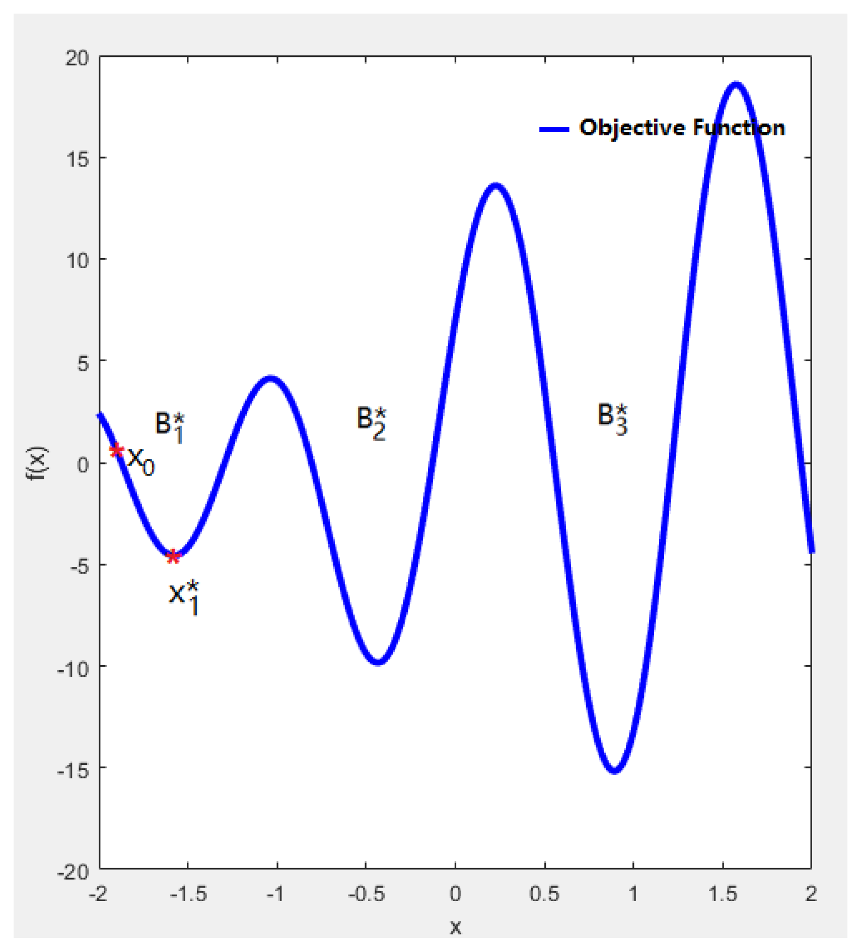
In the following, we use an example to demonstrate the optimization procedure of the filled function algorithm. Figure 1 shows the objective function $f\left(x\right)=x+10sin\left(5x\right)+7cos\left(4x\right)$ with the search region [−2, 2]. From Figure 1, we can see that $f\left(x\right)$ has three basins $B_1^{*}$, $B_2^{*}$ and $B_3^{*}$ in the search region, where $B_3^{*}$ is the lowest basin that contains the global optimal solution. Suppose the optimization procedure starts from $x_0$; using the BFGS local search method we can obtain a local minimal solution $x_1^{*}$ of the objective function $f\left(x\right)$.

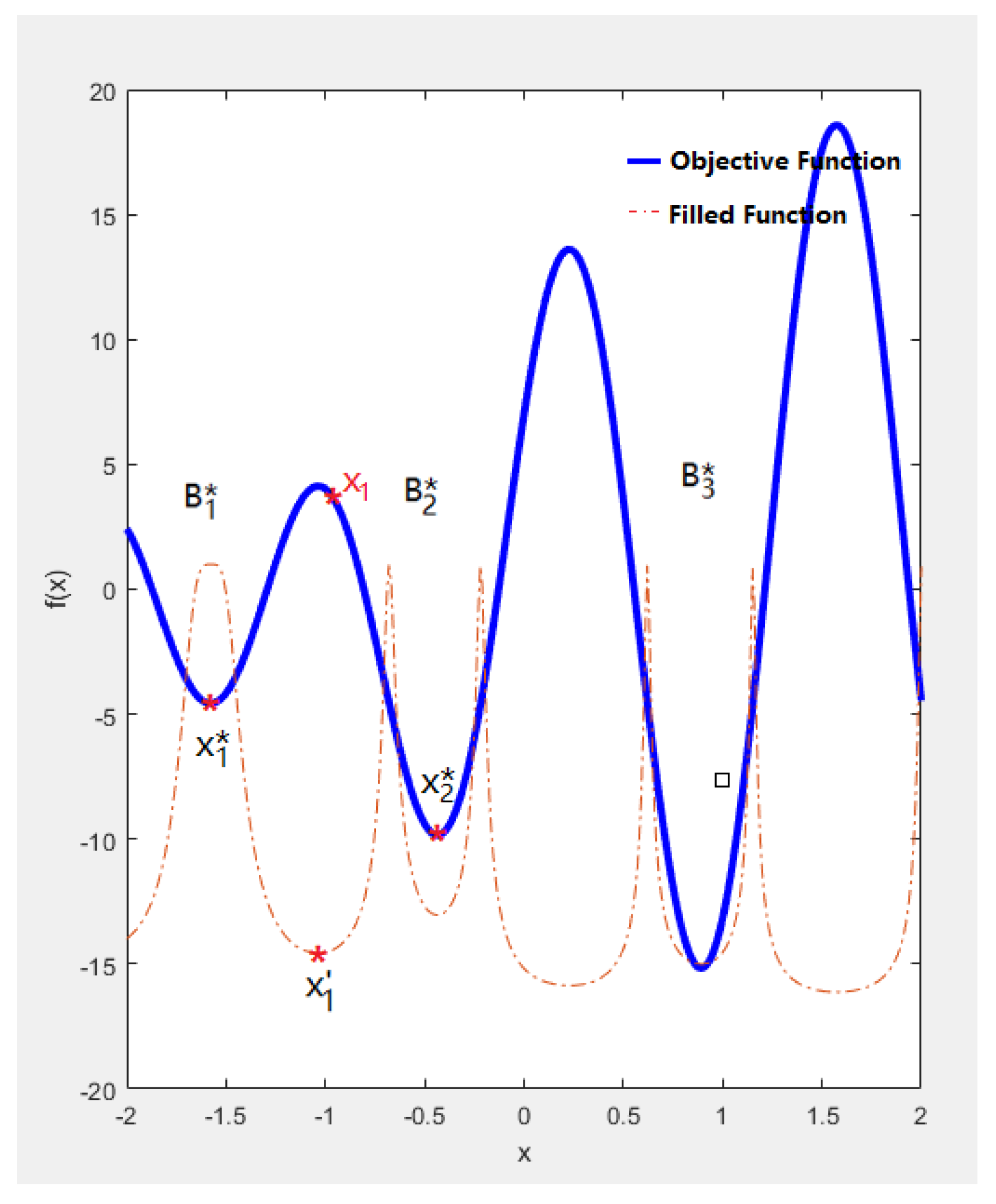
To escape from this local minimum $x_1^{*}$, we construct the filled function $P(x,x_1^{*})$ at $x_1^{*}$, as shown in Figure 2.

From Figure 2, we can see that $x_1^{*}$ is a strictly local maximum (maximal point) of $P(x,x_1^{*})$, which is guaranteed by the definition of the filled function. Therefore, a local search of $P(x,x_1^{*})$, starting from point $x_1^{*}+0.1$, can easily escape from this point and yield a local minima $x_1^{\prime }$ of $P(x,x_1^{*})$. Next, using $x_1(x_1=x_1^{\prime }+0.1)$ as the initial point to optimize the objective function $f\left(x\right)$, we can obtain another local minimal solution $x_2^{*}$ that is better than $x_1^{*}$. At this time, the first iteration is completed.

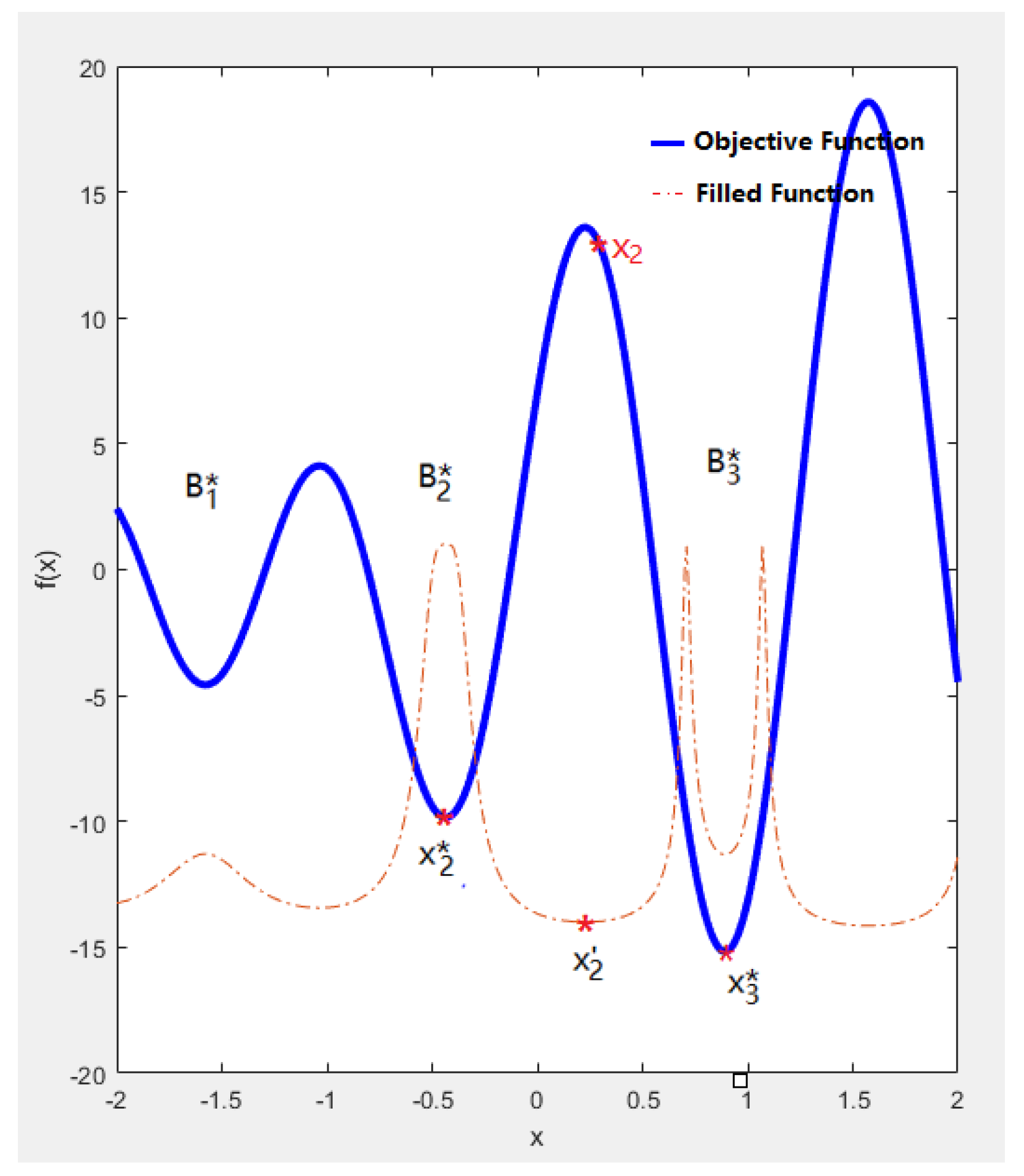
To escape from the local minimum $x_2^{*}$, we repeat the above steps to construct the filled function $P(x,x_2^{*})$ at $x_2^{*}$, as shown in Figure 3.

Similarly, $P(x,x_2^{*})$ peaks at point $x_2^{*}$, which makes it easy to escape from this point. We continue to optimize $P(x,x_2^{*})$ to obtain a local minimal point $x_2^{\prime }$. Then, using $x_2=x_2^{\prime }+0.1$ as the initial point to optimize the objective function $f\left(x\right)$, a new better local optimal solution $x_3^{*}$ is obtained. Now, the second iteration is completed. We continue the above procedure to optimize the objective function and filled function alternately to escape from the current local optimal solution to a better one till the global optimal solution is located.

From the above optimization procedure, we can clearly see that the proposed method can easily and continuously escape from a current local optimal solution to obtain a better one till the global optimal solution is located. This is a good way to overcome the disadvantage of premature convergence of optimization algorithms. Moreover, the proposed method also has three other advantages. First, since the proposed filled function is parameterless; the algorithm has no adjustable parameters to tune for different problems. Secondly, since the new filled function is continuous and differentiable, the proposed algorithm is less apt to produce an extra local minimum while more choices of local search methods, especially the efficient gradient-based ones, can be applied to make the optimization more efficient and effective. Thirdly, once the filled function is designed and constructed, it is easy to implement and apply to different optimization problems.

There are mainly two disadvantages of the filled function method. First, it is not easy to design a good filled function and each time when a local optimal solution is found, the filled function has to be constructed. Secondly, the filled function method becomes less effective when the dimensionality of the problem is large. More research is needed to extend the scope of the filled function method.

4. Numerical Experiments

The proposed filled function algorithm is implemented in Matlab 2021 and tested on wildly used test problems. Comparisons are made with a state-of-the-art filled function algorithm [18], another continuous differentiable filled function algorithm [5] and Ge’s filled function algorithm [1]. The test problems used in this paper are listed as follows.

Test case 1. (The rastrigin function)

$$\begin{array}{c}minF\left(x\right)=x_1^2+x_2^2-cos18x_1-cos18x_2\\ s.t.-3<x_1<3,-3<x_2<3\end{array}$$

The global minimum solution is $x^{*}={(0,0)}^T$, and the corresponding function value is $F\left(x^{*}\right)=-2$.

Test case 2. (Two-dimensional function)

$$\begin{array}{c}minF\left(x\right)={[1-2x_2+csin\left(4\pi x_2\right)-x_1]}^2+{[x_2-0.5sin\left(2\pi x_1\right)]}^2\\ s.t.0<x_1<10,-10<x_2<0\end{array}$$

where $c=0.05,0.2,0.5$. The global minimum solution is $x^{*}={(1,0)}^T$, and the corresponding function value is $F\left(x^{*}\right)=0$ for all values of c.

Test case 3. (Three-hump back camel function)

$$\begin{array}{c}minF\left(x\right)={2x}_1^2-1.05x_1^4+\frac{1}{6}{x}_1^6-x_1{x}_2+x_2^2\\ s.t.-3<x_1<3,-3<x_2<3\end{array}$$

The global minimum solution is $x^{*}={(0,0)}^T$, and the corresponding function value is $F\left(x^{*}\right)=0$.

Test case 4. (Six-hump back camel function)

$$\begin{array}{c}minF\left(x\right)={4x}_1^2-2.1x_1^4+\frac{1}{3}{x}_1^6-x_1{x}_2-4x_2^2+{4x}_2^4\\ s.t.-3<x_1<3,-3<x_2<3\end{array}$$

The global minimum solution is $x^{*}={(\pm 0.0898,\pm 0.7127)}^T$, and the corresponding function value is $F\left(x^{*}\right)=-1.0316$.

Test case 5. (Treccani function)

$$\begin{array}{c}minF\left(x\right)=x_1^4+4x_1^3+4x_1^2+x_2^2\\ s.t.-3<x_1<3,-3<x_2<3\end{array}$$

The global minimum solution is $x^{*}={(-2,0)}^T$ and $x^{*}={(0,0)}^T$, and the corresponding function value is $F\left(x^{*}\right)=0$.

Test case 6. ( Two-dimensional Shubert function)

$$\begin{array}{c}minF\left(x\right)=\left\{\sum _{i=1}^{5}icos\left[\left(i+1\right)x_1+i\right]\right\}\left\{\sum _{i=1}^{5}icos\left[\left(i+1\right)x_2+i\right]\right\}\\ s.t.0<x_1<10,0<x_2<10\end{array}$$

There are multiple local minimum solutions in the feasible region, and the global minimum function value is $F\left(x^{*}\right)=-186.7309$.

Test case 7. ( n-dimensional function)

$$\begin{array}{c}minF\left(x\right)=\frac{\pi }{n}[10{sin}^2\left(\pi x_1\right)+g\left(x\right)+{(x_n-1)}^2]\\ s.t.-10<x_i<10,i=1,2,\dots \dots ,n\end{array}$$

where

$$g\left(x\right)=\sum _{i=1}^{n-1}\left[{(x_i-1)}^2(1+10{sin}^2\left(\pi x_{i+1}\right))\right]$$

The global minimum solution is $x^{*}={(1,1,\dots ,1)}^T$, and the corresponding function value is $F\left(x^{*}\right)=0$ for all values of n.

First, all results obtained by the new filled function algorithm are listed in

Table 1. Results of Problem 1.

	Ours		CDFA
$\mathit{k}$	${\mathit{x}}_{\mathit{k}}^{*}$	${\mathit{f}}_{\mathit{k}}^{*}$	${\mathit{x}}_{\mathit{k}}^{*}$	${\mathit{f}}_{\mathit{k}}^{*}$
1	(${-0.7168,-0.0344)}^T$	−1.2439	/	/
2	(${-0.6938,0.0000)}^T$	−1.5156	/	/
3	($-0.7815\times {10}^{-7},-0.0179\times {10}^{-7}{)}^T$	−2.0000	/	/

,

Table 2. Results of Problem 2 (c = 0.2).

	Ours		CDFA
$\mathit{k}$	${\mathit{x}}_{\mathit{k}}^{*}$	${\mathit{f}}_{\mathit{k}}^{*}$	${\mathit{x}}_{\mathit{k}}^{*}$	${\mathit{f}}_{\mathit{k}}^{*}$
1	${(8.8344,-3.3354)}^T$	9.4093	${(5.7221,-1.8806)}^T$	2.5070
2	${(1.8784,-0.3458)}^T$	$1.9805\times {10}^{-15}$	${(3.7387,-1.2649)}^T$	0.6165
3			${(1.5909,-0.2703)}^T$	$2.8126\times {10}^{-9}$

,

Table 3. Results of Problem 2 (c = 0.5).

	Ours		CDFA
$\mathit{k}$	${\mathit{x}}_{\mathit{k}}^{*}$	${\mathit{f}}_{\mathit{k}}^{*}$	${\mathit{x}}_{\mathit{k}}^{*}$	${\mathit{f}}_{\mathit{k}}^{*}$
1	${(3.9733,-1.7709)}^T$	3.3347	${(0.0420,-0.0948)}^T$	0.5175
2	${(1.4513,0)}^T$	0.2264	(1.0000,0)${}^T$	$5.7949\times {10}^{-16}$
3	${(1.0000,0)}^T$	0

,

Table 4. Results of Problem 2 (c = 0.05).

	Ours		CDFA
$\mathit{k}$	${\mathit{x}}_{\mathit{k}}^{*}$	${\mathit{f}}_{\mathit{k}}^{*}$	${\mathit{x}}_{\mathit{k}}^{*}$	${\mathit{f}}_{\mathit{k}}^{*}$
1	${(4.0604,-2.1833)}^T$	7.2212	${(8.7299,-3.2965)}^T$	9.0733
2	${(1.8513,-0.4021)}^T$	$1.1414\times {10}^{-12}$	${(7.7280,-0.4022)}^T$	6.5031
3			${(1.8513,-0.4021)}^T$	$4.3885\times {10}^{-11}$

,

Table 5. Results of Problem 3.

	Ours		CDFA
$\mathit{k}$	${\mathit{x}}_{\mathit{k}}^{*}$	${\mathit{f}}_{\mathit{k}}^{*}$	${\mathit{x}}_{\mathit{k}}^{*}$	${\mathit{f}}_{\mathit{k}}^{*}$
1	${(-0.2565,-0.4722)}^T$	0.2289	${(-1.7476,-0.8738)}^T$	0.2986
2	${(-0.4064\times {10}^{-7},-0.3367\times {10}^{-7})}^T$	$3.0680\times {10}^{-15}$	${(-0.0000,-0.0000)}^T$	$4.0157\times {10}^{-10}$

,

Table 6. Results of Problem 4.

	Ours		CDFA
$\mathit{k}$	${\mathit{x}}_{\mathit{k}}^{*}$	${\mathit{f}}_{\mathit{k}}^{*}$	${\mathit{x}}_{\mathit{k}}^{*}$	${\mathit{f}}_{\mathit{k}}^{*}$
1	${(0.1021,0.5426)}^T$	−0.8448	${(-1.6071,0.5687)}^T$	2.1043
2	${(0.0898,0.7127)}^T$	−1.0316	${(0.0898,0.7127)}^T$	−1.0316

,

Table 7. Another results of Problem 4.

	Ours		CDFA
$\mathit{k}$	${\mathit{x}}_{\mathit{k}}^{*}$	${\mathit{f}}_{\mathit{k}}^{*}$	${\mathit{x}}_{\mathit{k}}^{*}$	${\mathit{f}}_{\mathit{k}}^{*}$
1	${(0.2434,-0.7892)}^T$	−0.5178	${(1.6071,-0.5687)}^T$	2.1043
2	${(-0.0898,-0.7127)}^T$	−1.0316	${(-0.0898,-0.7127)}^T$	−1.0316

,

Table 8. Results of Problem 5.

	Ours		CDFA
$\mathit{k}$	${\mathit{x}}_{\mathit{k}}^{*}$	${\mathit{f}}_{\mathit{k}}^{*}$	${\mathit{x}}_{\mathit{k}}^{*}$	${\mathit{f}}_{\mathit{k}}^{*}$
1	${(-0.9200,-1.0954)}^T$	2.1871	${(-1.0000,0)}^T$	1.0000
2	${(-0.7800\times {10}^{-8},-0.3252\times {10}^{-8})}^T$	$2.5397\times {10}^{-16}$	${(-0.0000,-0.0000)}^T$	$2.4048\times {10}^{-17}$

,

Table 9. Results of Problem 6.

	Ours		CDFA
$\mathit{k}$	${\mathit{x}}_{\mathit{k}}^{*}$	${\mathit{f}}_{\mathit{k}}^{*}$	${\mathit{x}}_{\mathit{k}}^{*}$	${\mathit{f}}_{\mathit{k}}^{*}$
1	${(1.2424,7.2516)}^T$	−6.0455	${(2.0467,2.0467)}^T$	0
2	${(5.4829,3.7723)}^T$	−52.0504	${(3.2800,4.8581)}^T$	−46.511
3	${(5.4892,4.8581)}^T$	−186.7309	${(4.2760,4.8581)}^T$	−79.411
4			${(5.4892,4.8581)}^T$	−186.7309

,

Table 10. Results of Problem 7 (n = 2).

	Ours		CDFA
$\mathit{k}$	${\mathit{x}}_{\mathit{k}}^{*}$	${\mathit{f}}_{\mathit{k}}^{*}$	${\mathit{x}}_{\mathit{k}}^{*}$	${\mathit{f}}_{\mathit{k}}^{*}$
1	${(-0.9500,-0.0717)}^T$	11.1395	/	/
2	${(1.0000,1.0000)}^T$	$7.7954\times {10}^{-14}$	/	/

,

Table 11. Results of Problem 7 (n = 3).

	Ours		CDFA
$\mathit{k}$	${\mathit{x}}_{\mathit{k}}^{*}$	${\mathit{f}}_{\mathit{k}}^{*}$	${\mathit{x}}_{\mathit{k}}^{*}$	${\mathit{f}}_{\mathit{k}}^{*}$
1	${(-0.5665,-4.3568,-2.8414)}^T$	147.6024	/	/
2	${(1.9900,1.0000,1.0000)}^T$	1.0367	/	/
3	${(1.0000,1.0000,1.0000)}^T$	$1.2257\times {10}^{-13}$	/	/

,

Table 12. Results of Problem 7 (n = 5).

	Ours		CDFA
$\mathit{k}$	${\mathit{x}}_{\mathit{k}}^{*}$	${\mathit{f}}_{\mathit{k}}^{*}$	${\mathit{x}}_{\mathit{k}}^{*}$	${\mathit{f}}_{\mathit{k}}^{*}$
1	${(4.5092,4.9506,-0.8846,-3.0831,5.4416)}^T$	165.8637	/	/
2	${(1.9900,1.0000,1.0000,1.0000,1.0000)}^T$	0.6220	/	/
3	${(1.0000,1.0000,1.0000,1.0000,1.0000)}^T$	$8.6588\times {10}^{-12}$	/	/

,

Table 13. Results of Problem 7 (n = 7).

	Ours		CDFA
$\mathit{k}$	${\mathit{x}}_{\mathit{k}}^{*}$	${\mathit{f}}_{\mathit{k}}^{*}$	${\mathit{x}}_{\mathit{k}}^{*}$	${\mathit{f}}_{\mathit{k}}^{*}$
1	$(2.1849,9.6164,-1.8296,0.5062,$ ${0.1504,4.9519,-5.0729)}^T$	359.2339	$(1.0000,1.0000,1.0000,1.0000,$ ${1.0000,1.0000,1.0000)}^T$	$2.3538\times {10}^{-13}$
2	$(1.0000,1.0000,1.0000,1.0000,$ ${1.0000,1.0000,1.0000)}^T$	$8.2241\times {10}^{-13}$

and

Table 14. Results of Problem 7 (n = 10).

	Ours		CDFA
$\mathit{k}$	${\mathit{x}}_{\mathit{k}}^{*}$	${\mathit{f}}_{\mathit{k}}^{*}$	${\mathit{x}}_{\mathit{k}}^{*}$	${\mathit{f}}_{\mathit{k}}^{*}$
1	$(6.2612,7.8479,2.3710,0.8488,$ $8.7385,0.0580,0.4644,7.5710,$ ${7.2606,2.2505)}^T$	359.2339	$(0.0101,0.0103,0.0103,0.0104,$ $0.0103,0.0102,1.0000,6.0000,$ ${6.0000,6.0000)}^T$	2.6653
2	$(1.0013,0.5326,-0.9803,1.0066,$ $1.0152,0.9937,0.5966,1.0802,$ ${0.9954,-0.1773)}^T$	1.8292	$(1.1615,1.1651,0.4418,0.9258,$ $0.9638,-0.4809,0.9926,6.0000,$ ${6.0000,6.0000)}^T$	2.4443
3	$(1.0000,1.0000,1.0000,1.0000,$ $1.0000,1.0000,1.0000,1.0000,$ ${1.0000,1.0000)}^T$	1.5113 × ${10}^{-13}$	$(1.9900,1.0000,1.0000,1.0000,$ $1.0000,1.0000,1.0000,6.0000,$ ${6.0000,6.0000)}^T$	0.4443
4			$(1.0000,1.0000,1.0000,1.0000,$ $1.0000,1.0000,1.0000,1.0000,$ ${1.0000,1.0000)}^T$	0

. Further, the comparisons are made with another continuous differentiable filled function algorithm, CDFA in [5]. In these tables, we use the following notations:

$x_k^{*}:$ the local minimum of the objective function in the $kth$ iteration.

$f_k^{*}:$ the function value of the objective function at $x_k^{*}$.

$k:$ the iteration counter.

$F_f:$ the total function evaluations of the objective function and the filled function.

CDFA: the filled function algorithm proposed in [5].

FFFA: the filled function algorithm proposed in [18].

Table 1, Table 2, Table 3, Table 4, Table 5, Table 6, Table 7, Table 8, Table 9, Table 10, Table 11, Table 12, Table 13 and Table 14 show the numerical results of the test problems in different test criteria (different parameters and different dimensions) obtained by the proposed filled function algorithm. In these tables, k means the iterations for the filled function algorithm to locate the global minimum solution $x^{*}$, $F\left(x^{*}\right)$ is the corresponding function value and n is the dimension of the test problem.

From the numerical results, we can see that the proposed filled function algorithm can locate all the global minima solutions successfully (some with a precision error of less than ${10}^{-10}$) and within small iterations.

For these test problems, we also listed the results of another continuous differentiable filled function algorithm, CDFA [5]. Since CDFA just carried out parts of the test problems, we use slashes ( / ) to indicate the missed values. From the comparison, we can see that for problem 2 (c = 0.2), we use one less iteration to locate a minimum solution with six orders of magnitude higher accuracy than CDFA. For problem 2 (c = 0.5), although we use one more iteration than CDFA, we successfully located the global minimum 0. For problem 2 (c = 0.05), we use one less iteration and obtain a better result than CDFA. For problem 3 we locate a better result (five orders of magnitude higher accuracy) than CDFA with the same iterations. For problems 5 and 7 (n = 7), our algorithm use one more iteration than CDFA. For problem 6 we use one less iteration to locate the global minimum than CDFA. For problem 7 (n = 10), although we use one less iteration, CDFA located the global minimum 0 while we get $1.51\times {10}^{-13}$. From the above analysis, we can achieve the comparison results that our algorithm has four wins (problem 2 with c = 0.2, c = 0.05, and problems 3 and 6), two losses (problems 5 and 7 with n = 7), and three ties (problem 2 with c = 0.5, and problems 4 and 7 with n = 10) out of the overall ten test problems. Therefore, we come to the conclusion that the proposed filled function algorithm is more effective than CDFA.

Comparisons are also made with a state-of-the-art filled function algorithm, FFFA [18] and Ge’s filled function [1]. The comparison results are listed in

Table 15. The overall comparisons.

$\mathit{No}.$	n	Ours		FFFA		Ge’s Filled Function
		$\mathit{k}$	${\mathit{F}}_{\mathit{f}}$	$\mathit{k}$	${\mathit{F}}_{\mathit{f}}$	$\mathit{k}$	${\mathit{F}}_{\mathit{f}}$
1	2	3	553	2	1255	4	21,276
2	2(c = 0.2)	2	392	3	1997	15	27,500
	2(c = 0.5)	3	470	4	1400	34	54,505
	2(c = 0.05)	2	493	4	3888	35	38,424
3	2	2	378	1	1789	32	92,498
4	2	2	277	1	1792	44	35,171
5	2	2	259	4	2089	14	15,759
6	2	2	484	4	3576	20	103,988
7	2	2	463	3	294	22	107,899
	3	3	962	3	510	6	248,407
	5	2	2287	5	12,681	16	1,229,860
	7	2	2590	2	811	21	1,443,686
	10	5	12,795	3	20,044	16	1,829,898

, where $No.$ is the number of test problems and n is the dimension, $F_f$ refers to the total number of function evaluations consumed to obtain the optimal solutions (minimum solutions for minimization problems).

Since all three filled function algorithms can find the global minimum solutions, we compare their efficiency by the total number of iterations and function evaluations consumed by each algorithm. From Table 15, we can see that for all test problems, our algorithm is much better than Ge’s algorithm. As for the comparison with FFFA, we can see that for test problems 1, 3 and 4, although our algorithm takes one more iteration to get the optimal solution, we use much fewer function evaluations. For problems 2, 5 and 6, our algorithm uses fewer iterations and fewer function evaluations than that of FFFA. For problem 7, we can see that for dimension $n=2$, our algorithm uses fewer iterations but more function evaluations than FFFA, for $n=3$ and $n=7$, our algorithm uses more function evaluations than that of FFFA, but for $n=5$ and $n=10$, our algorithm performs much better than that of FFFA. We can see that for $n=5$ our algorithm uses three fewer iterations and only uses 2287 function evaluations, while FFFA uses 12,681 function evaluations; for $n=10$, our algorithm only uses 12,795 function evaluations (which is nearly half of that of FFFA’s 20,044) to get the global optimal solution. Overall, we come to the conclusion that the filled function algorithm proposed in this paper is more efficient than FFFA. From the numerical results and comparison with the other three filled function algorithms, we come to the conclusion that the new filled function algorithm is effective and efficient for solving unconstrained global optimization problems.

5. An Application of the Filled Function Algorithm

In this section, the proposed filled function algorithm is applied to the supply chain problem. Supply chain problems can be divided into three types, namely manufacturer’s core supply chain, supplier core supply chain and seller core supply chain. In this paper, we mainly consider the manufacturer’s core supply chain. For the manufacturer’s core supply chain, there are multiple suppliers, multiple shippers, multiple generalized transportation methods, multiple sellers and one manufacturer. In this supply chain, the manufacturer uses different raw materials to produce various products that are sold by multiple sellers. The optimization objective of the supply chain is to minimize the total transportation cost.

We suppose there is a supply chain with a manufacturer as the core, one supplier and one kind of raw material required for production. The unit raw material cost of this kind of raw material supplied by the supplier is 2000 USD/t, the maximum supply is 5000 t, and all shippers can deliver it. The manufacturer produces only one product and requires 1.2 t of raw material per ton of product. There are two shippers, both of which can provide services of two generalized modes of transport. There are three sellers, and the order quantity of each seller must be strictly satisfied. The manufacturer initially has no inventory products, the production cost per unit product is 1000 USD, and the maximum production capacity is 4500 t. The relevant unit costs are shown in

Table 16. Unit transportation cost and maximum transportation capacity of shippers.

	Shippers	Shipper 1		Shipper 2
Mode of Transportation		Unit Cost (USD/ton)	Max Capacity (ton)	Unit Cost (USD/ton)	Max Capacity (ton)
Generalized transportion methood 1	Seller 1	220	1000	200	1500
	Seller 2	250		220
	Seller 3	210		210
Generalized transportion methood 2	Seller 1	180	1200	200	1000
	Seller 2	200		210
	Seller 3	210		220

,

Table 17. Sales capacity and unit sales cost.

	Seller 1	Seller 2	Seller 3
unit product cost of sales (USD/ton)	80	90	85
Product Demand (ton)	1000	1200	800

and

Table 18. Unit cost and maximum transportation capacity of shippers.

	Shippers	Shipper 1		Shipper 2
Mode of Transportation		Unit Cost (USD/ton)	Max Capacity (ton)	Unit Cost (USD/ton)	Max Capacity (ton)
Generalized transportion methood 1	supplier 1	180	2000	190	2500
Generalized transportion methood 2	supplier 2	210	2200	220	2000

.

The optimization model used here is:

$$\begin{array}{c}minZC=(216{\beta }_{1111}+252{\beta }_{1121}+228{\beta }_{1211}+264{\beta }_{1221})\times Q+\\ 3700x_{1111}+3740x_{1112}+3695x_{1113}+3660x_{1121}+3690x_{1122}+3695x_{1123}+\\ 3680x_{1211}+3710x_{1212}+3695x_{1213}+3680x_{1221}+3700x_{1222}+3705x_{1223}.\end{array}$$

The constraints are:

$$\begin{array}{cc}\hfill & Q\le 4500\hfill \\ \hfill & x_{1111}+x_{1112}+x_{1113}\le 1000\hfill \\ \hfill & x_{1121}+x_{1122}+x_{1123}\le 1200\hfill \\ \hfill & x_{1211}+x_{1212}+x_{1213}\le 1500\hfill \\ \hfill & x_{1221}+x_{1222}+x_{1223}\le 1000\hfill \\ \hfill & x_{1111}+x_{1121}+x_{1211}+x_{1221}=1000\hfill \\ \hfill & x_{1112}+x_{1122}+x_{1212}+x_{1222}=1200\hfill \\ \hfill & x_{1113}+x_{1123}+x_{1213}+x_{1223}=800\hfill \\ \hfill & 1.2\times Q\le 5000\hfill \\ \hfill & 1.2\times {\beta }_{1111}\times Q\le 2000\hfill \\ \hfill & 1.2\times {\beta }_{1121}\times Q\le 2200\hfill \\ \hfill & 1.2\times {\beta }_{1211}\times Q\le 2500\hfill \\ \hfill & 1.2\times {\beta }_{1221}\times Q\le 2000\hfill \\ \hfill & {\beta }_{1111}+{\beta }_{1121}+{\beta }_{1211}+{\beta }_{1221}=1\hfill \end{array}$$

where:

$$\begin{array}{c}Q=x_{1111}+x_{1112}+x_{1113}+x_{1121}+x_{1122}+x_{1123}+\\ x_{1211}+x_{1212}+x_{1213}+x_{1221}+x_{1222}+x_{1223}.\end{array}$$

where $x_{ijnk}$ are non-negative integers, $k=1,2,3;j=1,2;n=1,2;{\beta }_{1jnl}$ are non-negative numbers. The symbols used in the model are explained as follows:

$ZC$: Total supply chain cost;

$x_{ijnk}$: The number of $i$-th product delivered to the $k$-th seller use the $n$-th generalized transportation method by the $j$-th transporter;

${\beta }_{ijnk}$: The ratio of $j$-th transporter using the $n$-th generalized transportation method from the $l$-th supplier to the $r$-th raw material to the manufacturer’s demand for the kind of raw material.

It can be seen from the model that the objective function is nonlinear, and the constraints of suppliers and the transportation of raw materials are also nonlinear, so the model is a nonlinear mixed integer programming model.

We applied the proposed filled function algorithm to this supply chain model to optimize the total transportation cost. We used MATLAB2021b programming on a 64-bit Windows 10, Intel(R) Core(TM) i5-9400F CPU@2.90 GHz memory personal computer to calculate it, we executed 20 independent runs, and the results are listed in

Table 19. The optimization results.

${\mathit{x}}_{1113}$	${\mathit{x}}_{1121}$	${\mathit{x}}_{1122}$	${\mathit{x}}_{1213}$	${\mathit{x}}_{1222}$	${\mathit{\beta }}_{1111}$	${\mathit{\beta }}_{1211}$	$\mathit{ZC}\left(\mathit{million}\right)$
800	1000	200	0	1000	0.556	0.444	1171.8
423	1000	200	377	1000	0.556	0.444	1171.8
300	1000	200	500	1000	0.556	0.444	1171.8
17	1000	200	783	1000	0.556	0.444	1171.8
2	1000	200	798	1000	0.556	0.444	1171.8

.

Table 19 shows the optimization results of nonzero variables (the values of other variables are all 0). We can see that this supply chain has multiple optimal solutions. By careful observation, we can see that when $x_{1121}$, $x_{1122}$, $x_{1222}$, ${\beta }_{1111}$ and ${\beta }_{1211}$ are fixed to the values shown in Table 19, and $x_{1113}$ and $x_{1213}$ satisfy the following conditions:

$$x_{1113}+x_{1213}=800.$$

Therefore, the minimum transportation cost of this example is USD 1171.8 million. In this case, $x_{1122}=200$ means that the manufacturer in this supply chain should arrange shipper 1 to deliver 200 t of the product to the second seller using the second generalized mode of transportation. ${\beta }_{1211}=0.444$ means that the manufacturer should let shipper 2 complete 44.4 percent of the transportation task using generalized transportation method 2.

We compare our results with the results from ref. [20], the proposed filled function algorithm in this paper finds multiple optimal solutions and takes less computational time. From Table 19, we can see that our algorithm successfully finds five optimal solutions while the algorithm in [20] only finds single optimal solution $x^{*}=$ (0, 0, 800, 0, 1000, 200, 0, 0, 0, 0, 1000, 0), ${\beta }^{*}=(0.556,0,0.444,0)$. Moreover, the average running time of our algorithm is 1106 s, while the running time of [20] is 5128 seconds. Therefore, we can come to the conclusion that the filled function algorithm in this paper is more effective and efficient.

6. Conclusions

In this paper, we design a new filled function method to solve unconstrained global optimization problems. The new filled function has two advantages. First, it has no adjustable parameters to tune for different optimization problems; Secondly, the new filled function is continuous and differentiable, which are very good properties. These good properties mean the filled function is less apt to produce extra fake local minimum during the optimization; further, more choices of local search methods, especially some efficient gradient-based ones, can be applied to make the optimization more efficient and effective. The proposed filled function algorithm is tested on widely used benchmark problems and is also applied to a supply chain problem. Numerical experiments show the algorithm is effective and efficient. However, we also notice that the filled function algorithm become less effective with high dimensional optimization problems. The reason may lie in two aspects: First, the search space grows exponentially with the increase in the distention, and secondly, the local search method is not efficient enough for high dimensional problems. The time complexity of the proposed filled function algorithm is dependent on the local search method adopted. Since the filled function designed in this paper has the advantage of continuous and differentiable, the efficient gradient-based algorithm BFGS Quasi-Newton Method can be used in the proposed model. BFGS is well known for its fast super-linear convergence speed, although its time complexity is $O\left(n^2\right)$. This may be one of the reasons that when the optimization problem grows, its performance degrades. The proposed algorithm mainly helps the optimization process to repeatedly escape from local optimal solutions to better ones to locate the global optimal solution. In this process, a different local search method can be used. In our future work, we will continue to work on this issue and design new and better local search methods to make the filled function algorithm more efficient and perform better on higher dimensional problems.