Advances in Magnetic and Electromagnetic Technique Interpretation

Abstract

Magnetic and electromagnetic techniques have been applied successfully to mineral exploration discovery. Both techniques rely on inferring the distribution of subsurface physical properties based on ground, airborne or borehole field measurements. Consequently, interpretation methods relating field measurements to underground physical properties are key to geophysical method success. Over the last 15 years, with the evolution of computer processing techniques, interpretation methods have matured and have seen numerous developments, from approximate interpretation to 3D inversion. The recent study of the scientific literature on magnetic and electromagnetic interpretation followed by an analysis of the distribution of the publication of these studies publication (and the citation numbers quoted) outline the research on these topics. The majority of studies are on electromagnetism, with an emphasis on numerical modeling, approximations, superparamagnetism, and induced polarization. In magnetics, the most popular studies were on remanence magnetization inversion and Euler deconvolution. Studies applicable to both methods involved 3D inversion, artificial intelligence, and open-source software. The number of citations reveals a different picture than the number of publications, where the same categories are present but magnetic study citations dominate, indicating in general a time lag of 10 years. The results of this review may help direct future research in these areas.

1. Introduction

Magnetic techniques measure variations in the Earth’s magnetic field [1] and interpret these variations as changes in underground mineralogy [2]. Electromagnetic methods (EMs) [3], where natural and electric sources are being used, inform about subsurface conductivity/resistivity [4]. These techniques are widely used for mineral exploration [1,5], and rely on the measurement of an external field to infer properties of the subsurface. This implies that meaningful interpretation of the results is key to the successful application of these techniques. In the past, field anomalies were matched with simple geometrical models, analytic or scaled [6]. However, with the advancement of computer technology, various methods were developed to improve earlier models and better interpret field data. The second decade of the XXIe century, with the significant advances in technology [7,8], was an active period for the development of exploration geophysics-based interpretation. Technological evolution during this decade saw a consolidation of the computer-based advances in hardware: improved processors, increased memory size, and better networking. We also witnessed the increased popularity of Python as an object-oriented computer language, the advent of machine learning (ML), and finally artificial intelligence (AI).

In this paper, we review the impact of this evolution on the interpretation of magnetic and EM techniques over the last 15 years, since Refs. [1,5,9,10] cover the first decade of the 21st century. This review is based on scientific publications in the last fifteen years, principally the following technical journals: Geophysics, Exploration Geophysics, Geophysical Prospecting, and Minerals.

Magnetic- and EM-based interpretations are characterized by various assumptions, including the size of the geophysical survey and the known geology. For the magnetic data, there is an extended range of transformation methods, which enhance the particularities of the underlying geology. For isolated targets, parametric inversions are popular. For the EM methods, there are many proposed approximations, as well as the availability of extensive research on numerical modeling. Some of these methods are applied in EM 1D inversion, while the ultimate inversion is 3D based, presenting particular challenges for the interpretation of magnetic and data. Magnetic inversion is also extended to include remanent magnetization inversion while for EM, Superparamagnetism (SPM) and Induced Polarization (IP) effects have been added to the EM interpretation methods. There has also been research done to joint inversion, with the objective of combining different types of measurements to establish a unique image of the subsurface properties. Artificial intelligence is also becoming a topic of research while open-source software is gaining popularity.

2. Magnetic Transformations

There is a long tradition of developing methods to transform magnetic data into a form more conducive to interpretation. Ref. [11] describes the relations between currently available transformations and vectors and recommend requirements and pitfalls for their practical use. Ref. [12] describes the most commonly used terms for magnetic data and transformations and discusses how these terms should and should not be used.

2.1. Derivatives and Integrals

Derivatives and integrals are commonly used in magnetic interpretation as an intermediate product to enhance the geological response. Ref. [13] shows that, if the magnetization direction is known, the pseudogravity gradient tensor derived from magnetic field data enhances anomalies caused by deep sources in the same way as the gravity gradient tensor. The eigenvectors corresponding to the smallest eigenvalues help in estimating the strike directions of 2D geological structures. Ref. [14] introduces a new derivative operator which is a linear combination of the horizontal and vertical derivatives, normalized by the analytic signal amplitude. Ref. [15] proposes practical techniques to perform 3D and 2D integral transformations, which are accurate and flexible. These techniques transform the potential field components to potential, or potential-field gradient components to potential field components. This transformation is applied in the space domain using cubic B-splines. Ref. [16] re-establishes the relation between vertical and horizontal gradients of potential field data as a Hilbert transform pair. Ref. [17] demonstrates how pseudo-derivatives of different orders can be combined and applied to potential field data to produce a new filtered data set, less sensitive to noise and also shows details about source locations. Ref. [18] uses a variant of the Savitzky–Golay derivative filter to produce a robust method for estimating the second vertical derivative of 2D potential field data.

2.2. Reduction to the Pole

Ref. [19] presents a reformulation of reduction to the pole (RTP) of magnetic data at low latitudes and at the equator using equivalent sources which relocate magnetic anomalies peaks directly over causative bodies. The proposed method addresses both the theoretical difficulty of low-latitude instability and the practical issue of computational cost. Ref. [20] proposes a new transformation using magnetization inversion, investigating whether edge effects at low latitudes could be reduced. To compute RTP near the equator, Ref. [21] develops a novel algorithm based on a simple approximation of the frequency domain RTP operator, which is more efficient than the spatial-domain method and less sensitive to data noise.

2.3. Analytic Signal

To estimate the analytic signal, which is often used as an edge-detection filter, Ref. [22] introduces a modified version which is less dependent on the source magnetization vector for the contact and the dike models. Ref. [23] develops a new approach to study the normalized full gradient, by assessing the entropy of the normalized modulus of the analytic signal at each level of continuation. Ref. [24] develops a transformation from measured magnetic field amplitude to the field component along the geomagnetic field, which can be useful in highly conductive environments. Ref. [25] presents a new method based on the reciprocal of the analytic signal amplitude and its derivatives, to directly estimate the structural indices and location parameters of 2D magnetic data. Ref. [26] proves the existence of an equivalent layer having an all-positive magnetic-moment distribution for the case in which the magnetization direction of this layer is the same as that of the true sources, regardless of their magnetization. Using this constraint, a new iterative method is developed for estimating the total magnetization direction of 3D magnetic sources based on the equivalent-layer technique. Ref. [27] develops a new automatic method for 2D magnetic interpretation based on combinations of analytic signals of the logarithm of different order analytic signals. Ref. [28] proposes a transformation of the analytic-signal amplitude that is simpler to interpret as it gives a field that is independent of the magnetic inclination, dip, and the direction of any remanent magnetization, and can be used to estimate the magnetic susceptibility.

2.4. Edge Detector

Other edge detector techniques have been developed. Ref. [29] presents an edge detector method, based on the tilt angle of the total horizontal gradient, which enhances magnetic anomalies. Ref. [30] proposes the normalized anisotropy variance method, based on the concept of normalized standard deviation, to detect edges of potential-field anomalies. Ref. [31] suggests the modification of the total horizontal derivative and analytic signal filters by combining the amplitude spectra of fractional-order-derivative filters with ad hoc phase spectra. This method is designed for edge detection, particularly of deep sources, and offers effective noise suppression in processing magnetic data. To address the problem of the subsurface magnetization oblique to the geomagnetic field direction, Ref. [32] presents a new method for boundary extraction from magnetic field where the data are represented as a triangulated 3D surface. Using model studies, Ref. [33] quantifies the influences of source parameters on predicted edge locations using existing edge-detection methods. Ref. [34] presents edge-enhanced filters with minimal noise issues.

2.5. Euler Deconvolution

The Euler deconvolution technique helps with locating and identifying magnetic causative bodies. Ref. [35] examines the influence of applying low-pass filtering on magnetic data before estimating Euler deconvolution structural index. Ref. [36] proposes to estimate the Euler deconvolution source location on the normalized source strength. Ref. [37] interprets gridded potential field data by combining the horizontal ratio and Euler method. Ref. [38] develops a new method that minimizes to one per anomaly the number of source location estimates in Euler deconvolution. Ref. [39] proposes a multiridge Euler deconvolution, where Euler deconvolution is applied along ridges of potential fields. Ref. [40] studies the impact of low-pass filtering on structural index and depth estimates. Ref. [41] presents design rules that should be followed when applying Euler deconvolution method yielding misleading results if these rules are not respected. Ref. [42] evaluates a simple new method for depth, location, and dip estimates from RTP magnetic data. Ref. [43] discusses the uses and abuses of the structural index of the Euler method. Ref. [44] converts Euler’s equation to spherical coordinates. Then, for multipole point sources, the Euler equation can be solved directly, for a particular structural index. Ref. [45] estimates the location of thin dykes using a semiautomatic method. Ref. [46] compares methods for estimating magnetic source depths. Ref. [47] estimates the correct structural index to be used in Euler deconvolution using a new criterion. Ref. [48] uses RTP synthetic and field anomalies to estimate limitations of the 3D Euler deconvolution-derived estimates of source dip and volume. Ref. [49] improves solution accuracy of the Euler method by applying it iteratively. Ref. [50] proposes the Ratio-Euler, which does not involve high-order derivative and is more noise resistant. Ref. [51] proposes a generalized source-distance semi-automatic interpretation method and compares it to Euler deconvolution and Tilt-Euler methods. Ref. [52] presents a new version of the popular Euler’s equation method that is less affected by trends and easier to interpret. Ref. [53] reduces the Euler deconvolution forward matrix noise with a linear operator.

2.6. Remanent Magnetization (Remanence)

Magnetic response is affected by the magnetic susceptibility and remanent magnetization of geological bodies, the second being traditionally neglected. For cases where anomalies are affected by significant remanent magnetization, Ref. [54] proposes an interpretation approach based on the normalized source strength, which is calculated from magnetic gradient tensor eigenvectors. Ref. [55] develops a space-domain inversion approach which reduces remanent magnetization effects by using the amplitude of magnetic anomaly, the analytic signal, and the normalized source strength. For estimating the total magnetization direction of a magnetic source, Ref. [56] develops a simple cross-correlation-based method between the vertical derivative of the normalized source strength and the RTP magnetic fields. A similar objective is pursued in Ref. [57] which improves the MAX-MIN method using k-means clustering followed by Wiener filtering. Ref. [58] estimates the source magnetization by comparing the pseudo-gravity and the total gradient data. To interpret the data, Ref. [59] proposes a parameter called modified normalized source strength that is convenient and more stable at low latitudes. To determine the total magnetization direction, Ref. [60] computes the multiple correlation coefficients between the RTP field and the multiple direction-insensitive magnitude transforms.

2.7. Other Filters

Various filters are used in magnetic interpretation approximation. Refs. [61,62] introduce a method for the fast interpretation of magnetic vector and tensor field data, using the concept of potential field migration. Ref. [63] evaluates the data richness (a combination of geologic constraint, interpretability of aeromagnetic data, data acquisition and processing errors) quantitatively, which leads to a quantitative confidence of aeromagnetic map interpretation. Ref. [64] applies the surface curvature to aeromagnetic data, which provides information on the magnetic grid surface geometry and causative sources. Using various combinations of different forms of the local wavenumbers, Ref. [65] proposes an estimation of the depth and nature (structural index) of 2D magnetic sources. By minimizing the mismatch between observed data and an assumed model, Ref. [66] reports the development of an advanced filter for estimating the susceptibility. Ref. [67] introduces a new method for the calculation of the depth, location, and dip of thin dykes from RTP magnetic data. Ref. [68] demonstrates how, by reducing the noise-sensitivity of the wavelet transform, this technique can be used as a semi-automatic interpretation method. Ref. [69] proposes a new method for the interpretation of magnetic gradient tensor data. Ref. [70] develops a technique removing the effect of the magnetization direction on a dike magnetic anomaly, which removes the requirement of applying RTP before interpreting the anomaly. Ref. [71] shows the utility of the curvelet transformation for noise filtering and qualitative delineation of magnetic sources. Using the depth from extreme point imaging technique, Ref. [72] develops a framework for imaging the 3D magnetization vector. Ref. [73] develops a sequential approach to estimate the magnetization vector using normalized source strength inversion and Bayesian Monte Carlo method.

3. Magnetic Modeling and Parametric Inversion

Various magnetic geometrical models have been developed over the years and they have been used in parametric inversion. Ref. [74] revises and summarizes the current forward modeling methods for calculating gravity- and magnetic-field components and partial derivatives associated to a 2D polygonal body. Ref. [75] approximates terrain effects for airborne gravity gradient tensor and total magnetic field with fast Fourier transform technique. Ref. [76] develops a new analytical expression for polyhedron magnetic-gradient tensor. To model self-demagnetization of finite bodies of high magnetic susceptibility and arbitrary shapes, Ref. [77] develops a novel iterative method based on integral equation and Gauss-fast Fourier transform technique. Expressions are developed for the magnetic potential, vector, and gradient tensor due to a triaxial ellipsoid [78] and uniformly magnetized semi-infinite vertical cylinder [79]. To improve the efficiency of numerical simulations of 3D potential field anomalies, Ref. [80] develops an efficient 1D integration algorithm in the space-wavenumber domain. Ref. [81] develops an new analytic formulation for modeling the potential field response of a prism which may have application in 3D modeling.

Ref. [82] develops a simple method to determine, from a residual magnetic anomaly, the geometrical parameters of a buried source. To better characterize the parameters of the source, Ref. [83] develops a new approach involving 2D complex algebra. Ref. [84] uses a simple dike model to develop a non-linear 2D constrained inversion technique for magnetic data collected along flight lines using a simple dike model. Ref. [85] applies the standard particle swarm optimization algorithm to invert 2D magnetic data.

4. EM Approximations

Due to the complexity of EM methods and the data size of airborne electromagnetic (AEM) surveys, approximation methods are still being developed for interpretation. Ref. [86] models the frequency domain EM fields induced inside a conductive homogeneous half-space by an individual horizontal current ring. Ref. [87] proposes to use combinations of spatial gradients to detect a conductive body below conductive overburden or embedded in conductive material. Ref. [88] bases on the method called inverse Q-transform a pseudo-seismic approach to process time domain electromagnetic Method (TDEM) data. Ref. [89] calculates the underground secondary current using the tensor value response of Green’s function to evaluate the EM footprint as the volume of maximum contribution at the EM receiver. Ref. [90] proposes simplifying the display of AEM responses and introduces new tools to present and analyze large data sets. Using a wire loop conductor model, Ref. [91] compares different time domain EM system responses, defining a comprehensive geobandwidth representing the response strength over a range of time constants. Ref. [92] examines the TDEM response of a horizontal wire loop which is located in a conductive half-space. Ref. [93] examines the time-domain underground electric fields in a conductive half-space while the source is an horizontal magnetic dipole located at surface or buried within the earth. Ref. [94] obtains an analytic solution for the finite-length transmitter EM fields located in an homogeneous conducting medium. To extend the concept of smoke-ring which helps in understanding the distribution of currents in the subsurface, Ref. [95] calculates the current distribution in an half-space during a half-sine waveform. Ref. [96] develops analytic formulae for the transient electric field originating from a vertical magnetic dipole source, below a conductive half-space.

Ref. [97] applies to AEM data various common spatial derivatives procedures developed for potential field data. Another simple model parameter is the decay time constant or tau. Ref. [98] proposes the use of EM field ratios to estimate the properties of a mineral deposit while Ref. [99] proposes a new estimation method for the decay time constant. For imaging TDEM data, Ref. [100] develops a new EM field imaging technique based on multi-aperture data as well as Kirchhoff migration. Ref. [101] proposes a rapid method of calculating sensitivity functions of a homogeneous half-space model for various of transient EM configurations. Ref. [102] presents a new approximate forward modeling routine for 1D TDEM responses which can be integrated into an inversion formulation. Ref. [103] proposes a new technique for computing the sensitivity function along a profile by generating the maximum signal-to-noise ratio with a discrete conductor model.

For fixed in-loop EM surveys, Ref. [104] estimates the thin sheet local varying conductance through a simplified solution or through inversion. For borehole data, Ref. [105] estimates the thin sheet conductance from spatial and temporal derivatives. For interpreting AEM data, Ref. [106] compares the energy envelope and the vector magnitude. Ref. [107] develops a method for imaging ground TDEM data and extracting small conductor geometric parameters using secondary field spatial component combinations and Hilbert transforms. Using a dipole approximation, Ref. [108] shows the benefits of multi-component transmitter–receiver systems which allow the determination of target geometry. Ref. [109] proposes to interpret EM data collected in a resistive environment with magnetic dipole sources and apply their method to airborne data. Ref. [110] proposes to invert fixed-loop ground EM surveys with a combination of electric and magnetic dipoles. Using recent developments in spectral modeling, Ref. [111] presents fast 3D approximations of the EM response for simple geometry targets. Based on models of a magnetic dipole source, Ref. [112] proposes a topography correction for central loop helicopter data before 1D or 2D inversion, to improve depth estimations in mountainous areas. Ref. [113] presents a fast imaging technique for VLF EM data interpretation.

Following Ref. [114], who proposed the moment method for interpreting time domain surveys, Ref. [115] develops formulas for the moments of a one-dimensional earth with limited conductance. Ref. [116] proposes an analytic expression for the time integrals of magnetic responses of a rectangular-loop source over a conductive half-space. Ref. [117] extends these results to measurements below surface and is thus applicable to borehole measurements. Ref. [118] presents a rapid interpretation technique of AEM data based on the resistive limit. Ref. [119] develops a parametric thin-sheet variable algorithm for accurately modeling the conductivity structure of mineralization. Refs. [120,121,122] develop analytic expressions allowing the computation of the EM response of a sphere model located under a conductive overburden. Refs. [123,124] present another semi-analytic model of a sphere which is embedded in a layered earth, based on expansions of the spherical and cylindrical function derivatives. Ref. [125] develops a fast magnetostatic algorithm to compute the resistive limit response of an ellipsoidal conductor. From horizontal and vertical on-time EM components, Ref. [126] derives formulas to estimate the parameters of simple geometrical models located in a half-space or two-layer model. Ref. [127] develops a Bayesian framework allowing the inversion for conductors located in a layered earth and informing on the associated uncertainties, such as asserting if the data support a basement conductor model or not. Ref. [128] implements a 2.5D Bayesian inversion to invert ground TEM data.

5. EM Numerical Modeling

Improvements in EM numerical methods include developments in modeling techniques such as:

• Finite-element [129,130,131,132,133,134,135,136,137,138,139,140,141,142,143,144,145,146,147,148,149,150,151,152];
• Finite-difference [153,154,155,156,157];
• Finite-volume [158,159,160,161,162,163];
• Mimetic multiscale [164];
• Mimetic finite-volume [165];
• Hybrid integral equation-finite-element [166];
• Hybrid finite volume-integral equation [167];
• Spectral element method [168,169,170,171];
• Rapid expansion method [172];
• Radiation boundary method [173];
• Mixed space-number domain [174];
• Edge-element basis functions [175].

Ref. [176] compares finite-element and finite-volume while Ref. [177] compares nodal and edge finite-element basis functions. Algorithms for frequency to time-domain transformation are also investigated by Ref. [178]. Ref. [179] develops an inversion algorithm to transform TDEM data into frequency domain.

Refs. [180,181] introduce numerical solutions which include in EM modeling schemes the receiver geometry. This is in contrast with the usual approach, which assumes that measured electric fields are obtained over point-dipoles. Ref. [182] develops a finite-element approach for frequency-domain 3D CSEM forward modeling that can offer accurate EM responses for large-scale complex models. Ref. [183] introduces the meshless generalized finite-difference method, which has as advantages that only a discretization of points is required. Results compare favorably with existing methods. Ref. [184] studies anomalous diffusion of EM fields caused by fractal, porous, and canny rough media with 3D finite-difference models. They observe that the roughness of the media decreases the early-time EM signal and enhances the late-time response, slowing down EM field decay and diffusion.

6. EM 1D Inversion

The EM data size can be astronomic, particularly for airborne surveys. For this reason, and also due to the non-uniqueness inherent in EM inversions, 1D inversion was favored in the past. Ref. [185] studies the effects of inaccurate system description on 1D inverted models of helicopter TDEM data. Ref. [186] tries to reduce EM non-uniqueness due to equivalence for a thin conductive layer. Efforts are focused on improving inverted model lateral variations. Ref. [187] tests three kinds of regularization for 1D inversion of AEM data. Ref. [188] proposes a method for inverting single offset ground multifrequency EM data in 1D and 2D. Ref. [189] proposes a sharp spatially constrained inversion, where vertical and lateral smoothing constraints include sharp reconstruction of boundaries. Ref. [190] optimizes an inversion code for 1D inversion with very large-scale constraints. Ref. [191] develops 1D real-time approximations for circular central-loop configuration TDEM data. Ref. [192] develops a simulated annealing method to invert Semi-airborne Transient Electromagnetic method (SATEM) data with a 1D model. Ref. [193] applies supervised descent method to the 1D inversion of TDEM data. Ref. [194] combines on- and off-time data for inverting shallow structures. Ref. [195] details the use of the Kalman filter algorithm to solve AEM 1D inversion with lateral constraints. Ref. [196] describes a generalization of the well-known Tikhonov’s solution applied to 1D inversion of arbitrary source EM data.

Several authors propose a Bayesian approach to AEM 1D inversion. Ref. [197] develops a Bayesian parametric bootstrap approach which is a compromise between costly computer costs and efficient inversions. Ref. [198] proposes a transdimensional sampling approach to approximate a model of the subsurface. Ref. [199] develops a 2D airborne frequency-domain EM inversion algorithm, combining 1D and 2D inversions in a three-stage process. Ref. [200] proposes to invert in a probabilistic manner at various locations. The results are compared with deterministic inversions, from which the high-credibility regions are selected. Ref. [201] develops an adaptive laterally constrained inversion scheme, introducing user-defined constraints through a multivariate Gaussian prior within a Bayesian framework.

7. 3D Inversion

7.1. Generalities

The objective of geophysical interpretation in mineral exploration is to relate geophysical measurements to geological properties of the subsurface. This can be achieved by developing a 3D model of the subsurface and inferring the geological properties of this model. Ref. [202] shows that this process has evolved on various fronts for magnetic and EM techniques. First, several studies have been conducted either to improve property measurements [203,204,205,206] or to better understand the relations between physical properties and geology [207,208,209,210,211,212,213,214,215,216,217,218]. Second, developments in computer modeling have facilitated continuing improvement in computer performance. For example, Ref. [219] proposes to approximate the Jacobi matrix. Three-dimensional forward modeling can be carried out using rectilinear meshes [220], OcTree meshes [221,222], unstructured tetrahedral meshes [223,224,225,226], and wireframe surfaces [223,227]. The maximum number of cells is generally related to the limitations in computer capacities which are always expanding [228,229,230,231].

7.2. Magnetic

3D inversion techniques were first developed for the potential field methods. Ref. [232] presents a procedure to invert potential-field data by means of a flexible depth-weighting function representing the source field decay. Refs. [233,234,235] develop various approaches, sometimes using c-mean clustering or other clustering technique, to encourage the cell physical property to be near to a prescribed value, which can be dictated by the known statistical petrophysical data. Ref. [236] develops an approximate 3D inversion resolution measure not affected by the recovered model which give more realistic resolving lengths than provided by this model. For weak induced magnetization, Ref. [237] designs a multiple-set method for finding the boundaries of geometric shape of the causative bodies. While investigating self-magnetization effects, Ref. [238] compares total magnetization and magnetic amplitude inversions and show that the magnetic amplitude inversion is preferable for large susceptibility values. Ref. [239] develops two approaches for 3D magnetic sparse inversion taking advantage of outcrop or borehole susceptibility information. Ref. [240] proposes an adjustable exponential stabilizing functional to provide sharp petrophysical boundaries in potential field inversion. Ref. [241] constructs a reference model varying laterally and confined to superficial topography. Ref. [242] develops a magnetic amplitude inversion algorithm when self-demagnetization and remanent magnetization are present. Inversion of vector magnetic data is developed in 2.5D [243] and 3D [244].

7.3. Electromagnetic

3D inversion is quite complex for the EM techniques, particularly if the primary field geometry is different at each transmitter location. Ref. [245] reviews the development and applications of EM technology for mineral exploration, including 3D EM forward modeling and inversion. Strategies have been developed, particularly for airborne EM surveys, to consider multiple meshes to represent the whole model and for detailed inversion. This includes:

• The moving footprint strategy [246];
• The progression from coarse to detail meshes [161,221,247,248,249,250,251];
• A combination of 3D and 1D mesh [252,253];
• Wavelet-based inversion [254];
• Factorization in multisources [255];
• A combination of adaptive octree discretization, space-filing curves, and wavelets [256];
• Compressive inversion [257];
• Parametric hybrid inversion [258];
• Survey decomposition [259];
• Parameterization with block structures [260];
• Triple mesh formulation [261];
• Decoupled inversion and model grids: for model grid, columns of rectangular prisms arbitrarily are discretized in the vertical direction and appropriate horizontal smoothing is applied [262];
• Decoupled meshes for model mesh and Jacobian information [263];
• Backward-Euler direct splitting finite-difference [264];
• Subdomain decomposition [265].

Minimum-structure inversion [202] is still the preferred technique but has been improved in several ways, like by comparing the performance of different iterative solvers [266], mixing $l_p$ norms [267], or realizing stabilizers in a common setting [268]. Ref. [269] investigates a quite-fast convergent algorithm for 3D multipulse transient AEM data inversion based on direct Gauss–Newton optimization. Ref. [270] proposes to invert controlled-source audio MT data using a limited-memory method. Ref. [271] develops two inversion workflows sequentially inverting conductivity and susceptibility models. 3D inversion has also been adapted to semi-airborne EM systems [272]. For the inversion of EM data, Ref. [273] investigates surface geometry inversion.

8. Remanent Magnetization Inversion

Several approaches have been proposed in the last decade to map subsurface magnetization [274]. Ref. [275] stresses the importance of characterizing total and remanent magnetization. Ref. [276] develops two classes of approaches: (1) estimating total magnetization direction followed by incorporating the resultant direction into a known direction inversion algorithm; and (2) the direct inversion of the amplitude of the magnetic vector. Ref. [277] proposes new methods which estimate elementary model parameters from gradient tensor inversion. Ref. [278] proposes a strategy to invert magnetic data acquired over rugged elevation for a strong remanent magnetization source. Ref. [279] develops a 2D sequential inversion method of recovering the magnetization intensity, susceptibility and magnetization direction. Ref. [280] inverts for magnetization vector components, applies self-organizing maps to identify magnetization domains, then estimate direction scatter by a Fisher statistic. Another approach developed by Ref. [234] is to invert the total-field magnetic anomaly to obtain a model which is classified by fuzzy c-main to recover a 3D distribution of magnetization. Refs. [281,282] develop an automated strategy for determining the weighting parameters for clustering, and apply it to the estimation of magnetization directions and uncertainties. Instead Ref. [283] proposes an interaction algorithm to recover the magnetization direction from an estimation of the magnetization intensity. Ref. [284] imposes sparsity assumptions allowed by using a spherical formulation.

Ref. [285] uses the relationship between inclination and declination of the total magnetization direction to estimate the direction of remanent magnetization. Ref. [286] proposes a Fourier domain transformation separating magnetic anomalies into induced and remanent magnetization components. This approach assumes that each isolated source is homogeneous and is characterized by a uniform and specific Koenigsberger ratio. The solution proposed by Refs. [287,288,289,290] is to simultaneously invert induced and remanent magnetization while incorporating Gramian regularization. Ref. [291] quantifies, through parametric bootstrapping and equivalent source method, the 3D magnetization inversion error level. Ref. [292] estimates the total magnetization direction vector for an isolated source using an extension to the standard cross-correlation method while computing the RTP anomaly with the equivalent layer technique. Ref. [293] provides an overview of magnetization inversion state of the art with a set of case studies.

9. SPM and IP

SPM effects were first identified and described in AEM surveys by Ref. [294], with a proposed correction technique. These effects were modeled and predicted on various AEM systems by Refs. [295,296,297,298,299]. Ref. [300] develops analytical expressions for orthogonal SPM responses created by a circular-loop over a magnetically viscous subsurface.

Ref. [301] combines Warburg and exponential decay models to predict inductive IP response. Ref. [302] proposes a new methodology to collect, process, and invert for the distribution of chargeability using inductive sources and observations of magnetic fields in the frequency domain. Ref. [303] develops a new forward modeling technique for modeling chargeability TDEM response in 3D, while Refs. [304,305,306,307,308,309,310] develop procedures for inverting inductive source time domain IP data. Refs. [311,312] describe IP effects on AEM data, while Ref. [313] tests various methods to estimate SPM and IP effects on AEM data. Ref. [314] studies the robustness of inverting airborne TDEM data to extract Cole–Cole parameters using synthetic multiparametric modeling and inversion. Ref. [315] models 3D IP effects on TDEM based on the finite-element method. Ref. [316] explores the effects on the IP response of the switch-off time of the step or the ramp waveforms. To recover the SPM and IP responses of narrow superficial material, Refs. [317,318] use dispersive thin sheet responses to develop data fitting recursive algorithm. Ref. [319] proposes an “airborne IP (AIP) scanner”, based on data metrics and inversion misfit, to indicate locations of definitive AIP signals, areas with potential AIP signals, and areas with not AIP detected. Ref. [320] presents an original approach to invert AEM data for conductivity and chargeability models using a combination of hydrid finite difference and integral equation numerical methods. Ref. [321] analyzes the influence of IP effect on CSEM sounding curve by modeling 1D medium. Ref. [322] simultaneously samples resistivity and pseudochargeability in a Bayesian framework to develop decouple IP effects from TDEM data. Ref. [323] investigates the effect of IP phenomena on electric and magnetic field from a ground-wire TDEM source.

10. Joint and Cooperative Inversion

As inversion of magnetic or EM data is non-unique, there has been an effort to combine the inversion of different data sets to produce a coherent interpretation. Ref. [324] presents various existing methods. Ref. [325] includes first-arrival seismic travel-time and normalized cross-gradient constraints in a data-space joint inversion algorithm of magnetotelluric, gravity and magnetic data. Ref. [326] introduces Gramian spaces of model parameters and Gramian constraints to the joint inversion of multimodal geophysical data. This approach is applied by Ref. [327] to jointly invert potential field data. Ref. [328] develops an algorithm to jointly invert helicopter-borne EM, ground EM, and radiomagnetotelluric. Ref. [329] uses the fussy c-means clustering technique to jointly invert multiple geophysical data sets. Ref. [330] combines joint inversion and geology differentiation to identify geology units consistent with airborne gravity and magnetic data and prior geological information. To interpret airborne geophysical data, Ref. [331] proposes an algorithm of 3D probability geology differentiation using mixed norm joint inversion and physical property measurements. Ref. [332] presents a probabilistic approach for jointly inverting gravity gradient and magnetic data by using a cross-variance matrix to couple the physical property models. Ref. [333] jointly inverts potential field data with an unstructured mesh and Gramian constraints integrated in the objective function. Refs. [334,335] use a Gaussian mixture model in a framework, extended to multiple data sets, for petrophysically and geologically guided geophysical inversion. Ref. [336] applies the level-set method [237] for jointly inverting surface and borehole magnetic data.

11. Artificial Intelligence

In all areas of knowledge, AI has gained impetus, and it is also the case for geophysical exploration. AI has the potential of automating tedious tasks, with sometimes a large gain in time and size of data processed, but needs supervision. Various approaches have been developed over the years, often using generic tools applied to geophysical data. To perform aeromagnetic compensation, Ref. [337] develops a supervised neural network algorithm trained on low-altitude survey data. Ref. [338] estimates location and depth of lineament-type anomalies in aeromagnetic maps using convolutional neural. To estimate locations of magnetic anomalies, Ref. [339] proposes a global optimizing bat algorithm. Ref. [340] presents a novel global optimization algorithm to invert geomagnetic anomalies. Ref. [341] presents a novel algorithm clustering Euler deconvolution depth solutions. Refs. [342,343] propose AI based algorithms to image subsurface susceptibility from magnetic data.

Ref. [344] proposes to automate the process of removing coupling to man-made conductors in transient AEM surveys data using artificial neural network. Ref. [345] uses the wavelet neural network in the development of a three-stage workflow to remove motion-induced noise. Ref. [346] proposes a deep learning method to remove multisource noise in AEM data. Using a deep neural network, Ref. [347] introduces a new imaging method for AEM data. Ref. [348] develops a hybrid workflow, applied to 1D TDEM inversion, that combines deep learning techniques with least-squares optimization methods. Refs. [349,350] develops AEM 1D and 2D interpretation techniques using deep and recurrent neural networks, respectively. Ref. [351] proposes 3D inversion using a convolutional neural network. For frequency-domain AEM data, Ref. [352] proposes a 2D fast imaging method based on the U-net network. Ref. [353] integrates neural networks in an airborne TDEM inversion framework. Ref. [354] uses deep learning in the development of an integrated workflow for inverting airborne TDEM data.

Ref. [355] approximates the mapping from 2D MT response to the resistivity model using a deformable convolutional neural network. Ref. [356] automatically recognizes sferic signals and estimates resistivity from audio MT data using a deep neural convolution network. Ref. [357] filters MT noisy data using a deep learning technique, while Ref. [358] develops a deep temporal convolutional network for the strong elimination of controlled-source EM data. Deep learning is also used by Ref. [359] to accelerate magnetotelluric 2D forward modeling.

For the rapid and objective integration of multi-parameter Earth-science related databases, Ref. [360] uses the fuzzy partitioning Gustafson–Kessel cluster algorithm. Ref. [361] explores porphyry copper deposits in an airborne prospect with the fuzzy ordered weighted averaging method used as a straightforward knowledge-driven approach. Ref. [362] investigates, on a synthetic geological model, the performance of five different clustering methods used to identify geological units characterized by susceptibility, density and conductivity. Ref. [363] combines standard inversions of airborne magnetic and gravity gradient with a deep neural network to produce a cooperative inversion. Ref. [364] proposes a methodology for producing an mineral prospectivity map various geophysical and non-geophysical data sets. Ref. [365] infers surface geological structures from geophysical survey data using an automated approach.

12. Open-Source Software

While software is developed by various organizations, either proprietary, commercially distributed or available through the cloud, there has been a continuous effort to release open source software [366]. A summary of recent open-source programs for magnetic and electromagnetic techniques is given in Table 1.

Table 1. Open-source software with application.

Name	Applications	Language	Reference
SimPEG	Geophysical modeling and inversion	Python	[366,367,368,369,370,371]
PyGMI	Geoscience modeling and interpretation	Python	[372]
Harmonica	Potential field processing, modeling, & inversion	Python	[373]
IGMAS+	Potential field 3D numerical modeling & visualization	Java	[374,375]
GAMS	2D Fourier magnetic data processing	Python	[376]
Monogenic	Monogenic signal attributes	Python	[377,378]
empymod	1D EM dipole source response	Python	[379]
EMmod	1D EM vertical transverse isotropic medium	FORTRAN & Matlab	[380]
fdesign	digital filters for EM modeling	Python	[381]
matlabCSEM	1D EM dipole source response	Matlab	[382]
GA_AEM	Modeling and Inversion of AEM data in 1D	C++	[383]
TransdEM	EM 1D transdimensional Bayesian inversion	Julia	[384]
MTpy	Processing and imaging MT data sets	Python	[385]
sphere	EM Sphere below a conductive overburden	C++ & Python	[386]
MARE2DEM	2D EM Modeling	Fortran & Matlab	[387]
Multicolor-MG	3D natural source Modeling	Fortran	[388]
em3d-MT	3D radio-magnetotelluric Modeling	MATLAB	[389]

In parallel, Python libraries linked to commercial software have been released [390,391].

13. Discussion

13.1. Publications and Citations

The numerous references presented in this paper illustrate that research is very active in this field, as many scientific papers have being published in the last fifteen years. The computer technology advances have lent themselves naturally to solving a plethora of technical problems.

Figure 1, Figure 2, Figure 3 and Figure 4 present the distribution of these technical papers. Figure 1 classifies the papers into different categories and shows that most of the papers are on EM numerical modeling, followed by EM approximations, 3D inversion, SPM and IP, artificial intelligence, and in EM 3D inversion (in descending order). Figure 2 illustrates a preponderance of EM papers, as more papers discuss EM topics than magnetics or combined studies of both methods. We must also note that there are almost as many combined method (magnetic and EM) studies than solely magnetic studies.

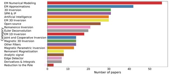
Figure 1. Number of papers classified by categories.

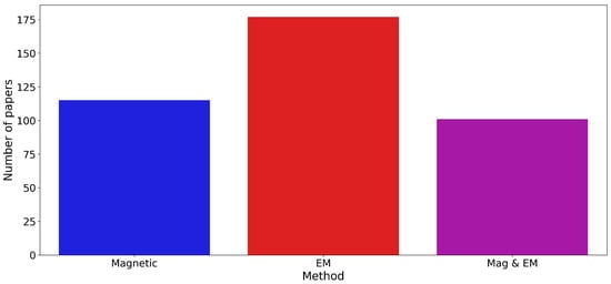
Figure 2. Number of studies by method.

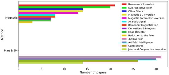
Figure 3. Number of papers on magnetics.

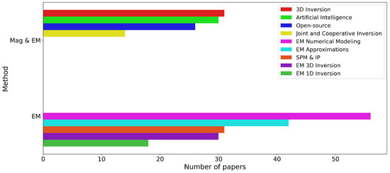
Figure 4. Number of papers on electromagnetics.

Detailed analysis of the distribution of studies on magnetic interpretation is shown in Figure 3, where remanence inversion and Euler deconvolution are the most studied topics. For EM interpretation, numerical modeling and EM approximations are the most popular topics. Among studies applicable to both methods, the largest number of studies discuss 3D inversion and artificial intelligence.

Our analysis of the popularity of the different methods is the following. EM Numerical modeling is by far the most studied problem, and we attribute that to the physical complexity of this problem. EM approximation studies follow, attributed to a corollary of the first observation, being that since EM modeling is complex, there is a clear benefit in EM approximations where the physics is simpler. This is followed by 3D inversion developed for both magnetic and EM. If we combine this number of articles with the number of articles on magnetic 3D inversion of EM 3D inversion, there is more research on 3D inversion than any other method. SPM and IP interpretation have gained popularity in EM interpretation since their observations in EM data. Artificial intelligence is a growing field, followed by open-source software.

In magnetic, remanence magnetization inversion is a growing field with various solutions proposed. This is followed by Euler deconvolution, which is preferred for its simplicity, albeit generating many solutions that must be filtered.

Another metric can be used to evaluate the popularity of these different methods. From Google Scholar, the citation numbers of these papers were estimated for 5 December 2025. Table 2 presents a list of the publications with more than 50 citations. Only one publication comes from the current decade, as all other publications were published between 2010 and 2017. There is a strong predominance of remanent magnetization inversion papers which is reflected in Figure 5 and Figure 6. Figure 5 illustrates that magnetic papers are more cited than EM papers, maybe a reflection of the larger community, while Figure 6 lists the various categories by the number of citations. Remanence magnetic inversion has the first rank, while the Euler deconvolution citation rank improves over its publication rank.

Table 2. Citation numbers (Google Scholar, 3 December 2025) from the publications discussed in this paper, showing only publications with more than 50 citations, sorted by decreasing citation number.

Citations	Reference	Year	Category
342	[276]	2010	Remanent magnetization inversion
274	[275]	2014	Remanent magnetization inversion
189	[277]	2012	Remanent magnetization inversion
103	[41]	2014	Euler Deconvolution
96	[233]	2015	Magnetic 3D Inversion
92	[43]	2014	Euler Deconvolution
84	[246]	2012	EM 3D Inversion
82	[230]	2014	Magnetic 3D Inversion
78	[234]	2016	Magnetic 3D Inversion
78	[293]	2021	Remanent Magnetization Inversion
78	[29]	2013	Edge Detector
74	[14]	2011	Derivatives & Integrals
73	[248]	2012	EM 3D Inversion
72	[62]	2012	Other filters
71	[221]	2014	3D Inversion
68	[54]	2013	Remanent Magnetization
68	[134]	2015	EM Numerical Modeling
67	[202]	2017	3D Inversion
67	[326]	2012	Joint Inversion
67	[38]	2013	Euler Deconvolution
65	[229]	2012	3D Inversion
61	[247]	2012	EM 3D Inversion
61	[74]	2011	Magnetic Modeling
59	[228]	2012	3D Inversion
58	[129]	2011	EM Numerical Modeling
56	[255]	2013	EM 3D Inversion
56	[385]	2014	Open-source
56	[61]	2012	Other filters
55	[101]	2014	EM Approximations
54	[223]	2012	3D Inversion
54	[37]	2013	Euler Deconvolution
53	[190]	2015	EM 1D Inversion
52	[30]	2014	Edge Detector
52	[132]	2014	EM Numerical Modeling
52	[280]	2016	Remanent Magnetization Inversion
51	[82]	2012	Magnetic Modeling

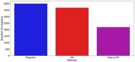
Figure 5. Number of citations by method.

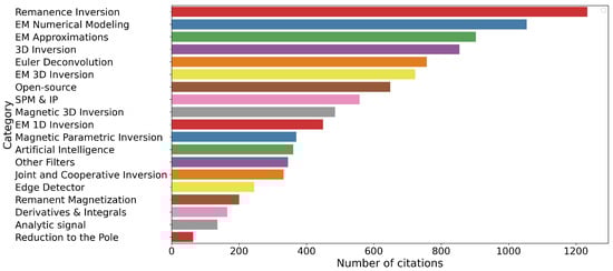
Figure 6. Number of citations for all the categories.

13.2. Challenges and Limitations

In this review, magnetic and EM methods have been treated separately, except for commonality in research or joint inversion, although modern exploration programs would benefit from some integration. The explorationist is faced with two problems that are related. First, which method should they follow among the near 400 publications cited in this paper? Then, which approach would lead to a better integration between magnetics and EM? Before proposing a solution, the following points must be considered.

Magnetic data are obtained from measurements of the variation in the Earth’s magnetic field associated to variation of the magnetic susceptibility and remanence of the subsurface. On the other hand, EM data represent secondary field measurements associated to an EM primary field, modified by the electrical property of the subsurface. First, field physics are completely different for the two methods, Laplace equation and Maxwell’s equations representing magnetic and EM fields respectively. This has a strong impact on field modeling, as EM fields are more difficult to represent numerically than the magnetic field, affecting the mathematical and computer requirements.

Secondly, since different fields are measured, techniques to collect these fields also vary and have evolved with technological evolution. The magnetic field measured can be a scalar or a vector, while EM fields are collected in a variety of transmitter and receiver combinations, in frequency or time domain. This implies the selection of the interpretation technique will be data dependent.

Finally, as pointed out before, the subsurface physical properties associated to these fields are different and characterize different geological environments. This implies that research on physical properties is key to interpretation, as its results can help to control interpretation, mainly by the use of constraint inversions, and improve interpretation relevance.

All these considerations imply that the selection of the method to use must be based on the objectives of the applications and the resources available. In this review, we do not try to compare the different methods presented, as this would require testing these methods on specific benchmarks. Instead, we recommend that the reader examine the theoretical models and examples presented by the authors of these papers and select the most appropriate for their needs. For example, if the object of the geophysical investigation is geological mapping using the magnetic method, then the Euler method, which is designed and more sensitive to discrete bodies, is not a good choice, and an edge detection technique will be more appropriate.

Time and computer resources are an important element of geophysical interpretation. Approximations methods, like magnetic transformations, magnetic modeling, EM approximation and 1D inversion, provide a limited image of the subsurface as their major strength is to work with limited resources (time and computer power). On the contrary, 3D modeling and inversion, particularly for EM methods, require extensive computer resources. Each method has is own strength, which is emphasizes by the examples that are shown for a particular study.

In summary, the validity of the various interpretation methods is determined by the justification of the numerical representation used to represent a geological environment, determined by the model selected, the model discretization, and the mathematical and computer tools available. This should be the criteria on which a given approach should be selected. Regarding the combination of magnetic and EM methods, the same rules apply, which implies that it is still a formidable task for the moment and cannot be applied everywhere.

14. Conclusions

The last fifteen years have seen many developments in the field of geophysical exploration for mineral deposits, particularly in the interpretation of magnetics and EM techniques. This has been mainly driven by advances in technology and geological understanding. The study of publications in magnetic and EM interpretation over these years reveals a strong research preference for EM numerical modeling and approximations, SPM, and IP studies. For magnetics, remanence magnetization inversion and Euler deconvolution are the most studied topics. For studies on 3D inversion, artificial intelligence, and open-source software, which apply to both methods, follow. On the opposite, if we consider the number of citations, magnetic study citations dominate.

One interesting aspect of our research is the observation of the time lag between the publications and the citations. Furthermore, except for the difference between magnetic and EM methods, in general the most popular topics are the most cited. Based on this observation, we propose that this study reflects the research directions in the near future. As technology continues to evolve, it is expected that the pace and complexity of research in these areas will also advance unabated, for the foreseeable future. Technology evolution and a better understanding of geological physical properties, limited by intrinsic physics and geophysical measurements, may lead to a better integration of these methods that would benefit modern exploration programs.

References

- Nabighian, M.N.; Grauch, V.J.S.; Hansen, R.O.; LaFehr, T.R.; Li, Y.; Peirce, J.W.; Phillips, J.D.; Ruder, M.E. The historical development of the magnetic method in exploration. Geophysics 2005, 70, 33ND–61ND. [Google Scholar] [CrossRef]
- Grant, F.S. Aeromagnetics, geology and ore environments, I. Magnetite in igneous, sedimentary and metamorphic rocks: An overview. Geoexploration 1985, 23, 303–333. [Google Scholar] [CrossRef]
- Zhdanov, M.S. Electromagnetic geophysics: Notes from the past and the road ahead. Geophysics 2010, 75, 75A49–75A66. [Google Scholar] [CrossRef]
- Palacky, G.J. Resistivity Characteristics of Geologic Targets. In Electromagnetic Methods in Applied Geophysics: Volume I, Theory; Nabighian, M.N., Ed.; Society of Exploration Geophysicists: Tulsa, OK, USA, 1987; pp. 53–129. [Google Scholar]
- Smith, R. Electromagnetic Induction Methods in Mining Geophysics from 2008 to 2012. Surv. Geophys. 2014, 35, 123–156. [Google Scholar] [CrossRef]
- Telford, W.M.; Geldart, L.P.; Sheriff, R.E.; Keys, D.A. Applied Geophysics; Cambridge University Press: London, UK, 1976. [Google Scholar]
- Hammond, A.C.R. The 20 Biggest Advances in Tech over the Last 20 Years; Foundation of Economic Education: Atlanta, GA, USA, 2020. [Google Scholar]
- Palandrani, P. A Decade of Change: How Tech Evolved in the 2010s an What’s in Store for the 2020s; Nasdaq: New York, NY, USA, 2022. [Google Scholar]
- Nabighian, M.N.; Asten, M.W. Metalliferous mining geophysics—State of the art in the last decade of the 20th century and the beginning of the new millennium. Geophysics 2002, 67, 964–978. [Google Scholar] [CrossRef]
- Vallée, M.A.; Smith, R.S.; Keating, P. Metalliferous mining geophysics—State of the art after a decade in the new millennium. Geophysics 2011, 76, W31–W50. [Google Scholar] [CrossRef]
- Li, X.; Pilkington, M. Attributes of the magnetic field, analytic signal, and monogenic signal for gravity and magnetic interpretation. Geophysics 2016, 81, J79–J86. [Google Scholar] [CrossRef]
- Bates, M.P.; Biegert, E.K.; Reid, A.B. Magnetic data—What am I looking at? Lead. Edge 2024, 43, 210–217. [Google Scholar] [CrossRef]
- Beiki, M.; Pedersen, L.B.; Nazi, H. Interpretation of aeromagnetic data using eigenvector analysis of pseudogravity gradient tensor. Geophysics 2011, 76, L1–L10. [Google Scholar] [CrossRef]
- Cooper, G.R.J.; Cowan, D.R. A generalized derivative operator for potential field data. Geophys. Prospect. 2011, 59, 188–194. [Google Scholar] [CrossRef]
- Wang, B.; Gao, S.S.; Liu, K.H.; Krebes, E.S. High-accuracy practical spline-based 3D and 2D integral transformations in potential-field geophysics. Geophys. Prospect. 2012, 60, 1001–1016. [Google Scholar] [CrossRef]
- Roy, I.G. An alternative approach in establishing relation between vertical and horizontal gradients of 2D potential field. Geophys. Prospect. 2017, 65, 1687–1693. [Google Scholar] [CrossRef]
- Cooper, G.R.J. A modified enhanced horizontal derivative filter for potential field data. Explor. Geophys. 2020, 51, 549–554. [Google Scholar] [CrossRef]
- Roy, I.G. Regularized 2D Savitzky–Golay derivative filter in estimating the second vertical derivative of potential field data. Geophys. Prospect. 2022, 70, 1066–1081. [Google Scholar] [CrossRef]
- Li, Y.; Nabighian, M.; Oldenburg, D.W. Using an equivalent source with positivity for low-latitude reduction to the pole without striation. Geophysics 2014, 79, J81–J90. [Google Scholar] [CrossRef]
- Lelièvre, P.G.; Fournier, D.; Walker, S.E.; Williams, N.C.; Farquharson, C.G. Research Note: A proposed procedure for ameliorating edge effects in magnetic data transformations. Geophys. Prospect. 2020, 68, 1999–2006. [Google Scholar] [CrossRef]
- Luo, Y.; Wu, M. Reduction to the pole near the equator with a Fourier-domain equivalent dipole layer. Geophysics 2023, 88, G115–G124. [Google Scholar] [CrossRef]
- Cooper, G.R.J. Reducing the dependence of the analytic signal amplitude of aeromagnetic data on the source vector direction. Geophysics 2014, 79, J55–J60. [Google Scholar] [CrossRef]
- Florio, G.; Fedi, M. Depth estimation from downward continuation: An entropy-based approach to normalized full gradient. Geophysics 2018, 83, J33–J42. [Google Scholar] [CrossRef]
- Zhen, H.; Li, Y.; Yang, Y. Transformation from total-field magnetic anomaly to the projection of the anomalous vector onto the normal geomagnetic field based on an optimization method. Geophysics 2019, 84, J43–J55. [Google Scholar] [CrossRef]
- Wang, Y.; Luo, X.; Zhang, J. Interpretation of 2D magnetic sources based on the reciprocal of the analytic signal amplitude. Explor. Geophys. 2019, 50, 645–652. [Google Scholar] [CrossRef]
- Reis, A.L.A.; Oliveira, V.C., Jr.; Barbosa, V.C.F. Generalized positivity constraint on magnetic equivalent layers. Geophysics 2020, 85, J99–J110. [Google Scholar] [CrossRef]
- Wang, Y.; Ding, Y.; Ai, H. Estimation of 2D magnetic-source parameters using analytic signals of the logarithm of different order analytic signals. Explor. Geophys. 2022, 53, 314–328. [Google Scholar]
- Smith, R.S.; Roots, E.A.; Vavanur, R. Transformation of magnetic data to the pole and vertical dip and a related apparent susceptibility transform: Exact and approximate approaches. Geophysics 2022, 87, G1–G14. [Google Scholar] [CrossRef]
- Ferreira, F.J.F.; de Souza, J.; de B. e S. Bongiolo, A.; de Castro, L.G. Enhancement of the total horizontal gradient of magnetic anomalies using the tilt angle. Geophysics 2013, 78, J33–J41. [Google Scholar] [CrossRef]
- Zhang, H.L.; Ravat, D.; Marangoni, Y.R.; Hu, X.Y. NAV-Edge: Edge detection of potential-field sources using normalized anisotropy variance. Geophysics 2014, 79, J43–J53. [Google Scholar]
- Arısoy, M.Ö.; Dikmen, Ü. Edge enhancement of magnetic data using fractional-order-derivative filters. Geophysics 2015, 80, J7–J17. [Google Scholar]
- Foks, N.L.; Li, Y. Automatic boundary extraction from magnetic field data using triangular meshes. Geophysics 2016, 81, J47–J60. [Google Scholar] [CrossRef]
- Pilkington, M.; Tschirhart, V. Practical considerations in the use of edge detectors for geologic mapping using magnetic data. Geophysics 2017, 82, J1–J8. [Google Scholar] [CrossRef]
- Cooper, G.R.J. Amplitude-balanced edge detection filters for potential field data. Explor. Geophys. 2023, 54, 544–552. [Google Scholar] [CrossRef]
- Davis, K.; Li, Y.; Nabighian, M.N. Effects of low-pass filtering on the calculated structural index from magnetic data. Geophysics 2011, 76, L23–L28. [Google Scholar] [CrossRef]
- Beiki, M.; Clark, D.A.; Austin, J.R.; Foss, C.A. Estimating source location using normalized magnetic source strength calculated from magnetic gradient tensor data. Geophysics 2012, 77, J23–J37. [Google Scholar] [CrossRef]
- Ma, G. Combination of horizontal gradient ratio and Euler methods for the interpretation of potential field data. Geophysics 2013, 78, J53–J60. [Google Scholar] [CrossRef]
- Melo, F.F.; Barbosa, V.C.F.; Uieda, L.; Oliveira, V.C., Jr.; Silva, J.B.C. Estimating the nature and the horizontal and vertical positions of 3D magnetic sources using Euler deconvolution. Geophysics 2013, 78, J87–J98. [Google Scholar] [CrossRef]
- Florio, G.; Fedi, M. Multiridge Euler deconvolution. Geophys. Prospect. 2014, 62, 333–351. [Google Scholar] [CrossRef]
- Florio, G.; Fedi, M.; Pašteka, R. On the estimation of the structural index from low-pass filtered magnetic data. Geophysics 2014, 79, J67–J80. [Google Scholar] [CrossRef]
- Reid, A.B.; Ebbing, J.; Webb, S.J. Avoidable Euler Errors—The use and abuse of Euler deconvolution applied to potential fields. Geophys. Prospect. 2014, 62, 1162–1168. [Google Scholar] [CrossRef]
- Cooper, G.R.J. The automatic determination of the location, depth, and dip of contacts from aeromagnetic data. Geophysics 2014, 79, J35–J41. [Google Scholar] [CrossRef]
- Reid, A.B.; Thurston, J.B. The structural index in gravity and magnetic interpretation: Errors, uses, and abuses. Geophysics 2014, 79, J61–J66. [Google Scholar] [CrossRef]
- Cooper, G.R.J. Euler deconvolution in a radial coordinate system. Geophys. Prospect. 2014, 62, 1169–1179. [Google Scholar] [CrossRef]
- Cooper, G.R.J. Using the analytic signal amplitude to determine the location and depth of thin dikes from magnetic data. Geophysics 2015, 80, J1–J6. [Google Scholar] [CrossRef]
- Cooper, G.R.J.; Whitehead, R.C. Determining the distance to magnetic sources. Geophysics 2016, 81, J25–J34. [Google Scholar] [CrossRef]
- Melo, F.F.; Barbosa, V.C.F. Correct structural index in Euler deconvolution via base-level estimates. Geophysics 2018, 83, J87–J98. [Google Scholar] [CrossRef]
- Amaral Mota, E.S.; Medeiros, W.E.; Oliveira, R.G. Can Euler deconvolution outline three-dimensional magnetic sources? Geophys. Prospect. 2020, 68, 2271–2291. [Google Scholar] [CrossRef]
- Cooper, G. Iterative Euler deconvolution. Explor. Geophys. 2021, 52, 468–474. [Google Scholar] [CrossRef]
- Huang, L.; Zhang, H.; Li, C.-F.; Feng, J. Ratio-Euler deconvolution and its applications. Geophys. Prospect. 2022, 70, 1016–1032. [Google Scholar] [CrossRef]
- Cooper, G.R.J. A generalized source-distance semi-automatic interpretation method for potential field data. Geophys. Prospect. 2023, 71, 713–721. [Google Scholar] [CrossRef]
- Cooper, G.R.J. Using Euler Deconvolution as Part of a Mineral Exploration Project. Minerals 2024, 14, 393. [Google Scholar] [CrossRef]
- Zhang, H.; Li, H.; Hu, X. An improved weighting Euler deconvolution for noisy data. Geophysics 2025, 90, G129–G138. [Google Scholar] [CrossRef]
- Pilkington, M.; Beiki, M. Mitigating remanent magnetization effects in magnetic data using the normalized source strength. Geophysics 2013, 78, J25–J32. [Google Scholar] [CrossRef]
- Guo, L.; Shi, L.; Meng, X.; Gao, R.; Chen, Z.; Zheng, Y. Apparent magnetization mapping in the presence of strong remanent magnetization: The space-domain inversion approach. Geophysics 2016, 81, J11–J24. [Google Scholar] [CrossRef]
- Zhang, H.; Ravat, D.; Marangoni, Y.R.; Chen, G.; Hu, X. Improved total magnetization direction determination by correlation of the normalized source strength derivative and the reduced-to-pole fields. Geophysics 2018, 83, J75–J85. [Google Scholar] [CrossRef]
- Wang, T.; Liu, S.; Zuo, B.; Hu, X. Improved MAX-MIN method to estimate total magnetization direction using Wiener filtering. Geophysics 2022, 87, G137–G156. [Google Scholar] [CrossRef]
- Hekmatian, M.E. Estimating the direction of source magnetisation through comparison of pseudogravity and total gradient. Explor. Geophys. 2019, 50, 193–209. [Google Scholar] [CrossRef]
- Hu, M.; Yu, P.; Zhang, L.; Zhao, C. Calculation of normalized source strength using second derivatives of the vertical integral of total-field magnetic anomaly. Geophysics 2022, 87, G97–G101. [Google Scholar] [CrossRef]
- Jian, X.; Liu, S.; Hu, X.; Zhang, Y.; Zhu, D.; Zuo, B. A new method to estimate the total magnetization direction from the magnetic anomaly: Multiple correlation. Geophysics 2022, 87, G115–G135. [Google Scholar] [CrossRef]
- Zhdanov, M.S.; Cai, H.; Wilson, G.A. Migration transformation of two-dimensional magnetic vector and tensor fields. Geophys. J. Int. 2012, 189, 1361–1368. [Google Scholar] [CrossRef][Green Version]
- Zhdanov, M.S.; Liu, X.; Wilson, G.A.; Wan, L. 3D migration for rapid imaging of total-magnetic-intensity data. Geophysics 2012, 77, J1–J5. [Google Scholar] [CrossRef]
- Aitken, A.R.A.; Holden, E.-J.; Dentith, M.C. Semiautomated quantification of the influence of data richness on confidence in the geologic interpretation of aeromagnetic maps. Geophysics 2013, 78, J1–J13. [Google Scholar] [CrossRef]
- Lee, M.; Morris, W.; Leblanc, G.; Harris, J. Curvature analysis to differentiate magnetic sources for geologic mapping. Geophys. Prospect. 2013, 61, 572–585. [Google Scholar] [CrossRef]
- Ma, G.; Li, L. Alternative local wavenumber methods to estimate magnetic source parameters. Explor. Geophys. 2013, 44, 264–271. [Google Scholar] [CrossRef]
- Ganguli, S.S.; Nayak, G.K.; Vedanti, N.; Dimri, V.P. A regularized Wiener–Hopf filter for inverting models with magnetic susceptibility. Geophys. Prospect. 2016, 64, 456–468. [Google Scholar] [CrossRef]
- Cooper, G.R.J. Applying the tilt-depth and contact-depth methods to the magnetic anomalies of thin dykes. Geophys. Prospect. 2017, 65, 316–323. [Google Scholar] [CrossRef]
- Cooper, G.R.J. Locating thin dykes using wavelet analysis of their magnetic anomalies. Explor. Geophys. 2019, 50, 554–560. [Google Scholar] [CrossRef]
- Li, J.; Zhang, Y.; Fan, H.; Li, Z.; Liu, M. Estimating the location of magnetic sources using magnetic gradient tensor data. Explor. Geophys. 2019, 50, 600–612. [Google Scholar] [CrossRef]
- de Souza, J.; Saulo Pomponet Oliveira, S.P.; Ferreira, F.J.F. Using parity decomposition for interpreting magnetic anomalies from dikes having arbitrary dip angles, induced and remanent magnetization. Geophysics 2020, 85, J51–J58. [Google Scholar] [CrossRef]
- Amirpour Asl, A.; Shad Manaman, N. Application of the curvelet transform to synthetic and real magnetic data. Explor. Geophys. 2020, 51, 285–299. [Google Scholar] [CrossRef]
- Shu, Y.; Liu, S.; Yan, J.; Zhou, Z.; Cai, H.; Hu, X. Magnetization vector depth from extreme points imaging for magnetic data. Geophysics 2025, 90, G167–G186. [Google Scholar] [CrossRef]
- Sun, S.; Xu, H.; Zhang, Q.; Meng, Q.; Cao, J. Estimation of magnetization directions using a sequential approach with inversion of normalized source strength and Bayesian Monte Carlo method. Geophysics 2025, 90, G109–G127. [Google Scholar] [CrossRef]
- Jia, Z.; Wu, S. Potential fields and their partial derivatives produced by a 2D homogeneous polygonal source: A summary with some revisions. Geophysics 2011, 76, L29–L34. [Google Scholar] [CrossRef]
- Pedersen, L.B.; Bastani, M.; Kamm, J. Gravity gradient and magnetic terrain effects for airborne applications—A practical fast Fourier transform technique. Geophysics 2015, 80, J19–J26. [Google Scholar] [CrossRef]
- Ren, Z.; Chen, H.; Chen, C.; Zhong, Y.; Tang, J. New analytical expression of the magnetic gradient tensor for homogeneous polyhedrons. Geophysics 2019, 84, A31–A35. [Google Scholar] [CrossRef]
- Ouyang, F.; Chen, L. Iterative magnetic forward modeling for high susceptibility based on integral equation and Gauss-fast Fourier transform. Geophysics 2020, 85, J1–J13. [Google Scholar] [CrossRef]
- McKenzie, K.B. The magnetic gradient tensor of a triaxial ellipsoid, its derivation and its application to the determination of magnetisation direction. Explor. Geophys. 2020, 51, 609–641. [Google Scholar] [CrossRef]
- Blair McKenzie, K. The magnetic field and magnetic gradient tensor for a right circular cylinder. Explor. Geophys. 2022, 53, 329–358. [Google Scholar] [CrossRef]
- Dai, S.; Chen, Q.; Li, K.; Ling, J. The forward modeling of 3D gravity and magnetic potential fields in space-wavenumber domains based on an integral method. Geophysics 2022, 87, G83–G96. [Google Scholar] [CrossRef]
- Boulanger, O. 2D fast Fourier transform analytical solutions in all space for all gravity and magnetic components. Geophys. Prospect. 2024, 72, 809–832. [Google Scholar] [CrossRef]
- Abdelrahman, E.S.M.; Abo-Ezz, E.R.; Essa, K.S. Parametric inversion of residual magnetic anomalies due to simple geometric bodies. Explor. Geophys. 2012, 43, 178–189. [Google Scholar] [CrossRef]
- Le Maire, P.; Munschy, M. 2D potential theory using complex algebra: New equations and visualization for the interpretation of potential field data. Geophysics 2018, 83, J1–J13. [Google Scholar] [CrossRef]
- Beiki, M.; Pedersen, L.B. Estimating magnetic dike parameters using a non-linear constrained inversion technique: An example from the Särna area, west central Sweden. Geophys. Prospect. 2012, 60, 526–538. [Google Scholar] [CrossRef]
- Liu, S.; Liang, M.; Hu, X. Particle swarm optimization inversion of magnetic data: Field examples from iron ore deposits in China. Geophysics 2018, 83, J43–J59. [Google Scholar] [CrossRef]
- Machado, M.V.B.; Dias, C.A. Zone of main contribution to the measured signal for a circular current loop source and receiver on the surface of a conductive half-space. Geophys. Prospect. 2012, 60, 1167–1185. [Google Scholar] [CrossRef]
- Smith, R.S. Using combinations of spatial gradients to improve the detectability of buried conductors below or within conductive material. Geophysics 2013, 78, E19–E31. [Google Scholar] [CrossRef]
- Xue, G.Q.; Gelius, L.-J.; Xiu, L.; Qi, Z.P.; Chen, W.Y. 3D pseudo-seismic imaging of transient electromagnetic data—A feasibility study. Geophys. Prospect. 2013, 61, 561–571. [Google Scholar] [CrossRef]
- Yin, C.; Huang, X.; Liu, Y.; Cai, J. Footprint for frequency-domain airborne electromagnetic systems. Geophysics 2014, 79, E243–E254. [Google Scholar] [CrossRef]
- Combrinck, M. Developing an efficient modelling and data presentation strategy for ATDEM system comparison and survey design. Explor. Geophys. 2015, 46, 3–11. [Google Scholar] [CrossRef]
- Hodges, G.; Chen, T. Geobandwidth: Comparing time domain electromagnetic waveforms with a wire loop model. Explor. Geophys. 2015, 46, 58–63. [Google Scholar] [CrossRef]
- Swidinsky, A.; Nabighian, M. On smoke rings produced by a loop buried in a conductive half-space. Geophysics 2015, 80, E225–E236. [Google Scholar] [CrossRef]
- Swidinsky, A.; Nabighian, M. Transient electromagnetic fields of a buried horizontal magnetic dipole. Geophysics 2016, 81, E481–E491. [Google Scholar] [CrossRef]
- Flekkøy, E.G.; Carneiro, M.V. An exact solution for the transient electromagnetic field around a finite-length transmitter. Geophysics 2017, 82, E51–E56. [Google Scholar] [CrossRef]
- Smiarowski, A.; Hodges, G. Transient electromagnetic smoke rings in a half-space during active transmitter excitation. Geophysics 2021, 86, E199–E208. [Google Scholar] [CrossRef]
- Fullagar, P.K. Smoke rings re-visited: An analytic solution for the transient electric field produced by a vertical magnetic dipole on or in a homogeneous conductive half-space. Explor. Geophys. 2022, 53, 591–601. [Google Scholar] [CrossRef]
- Beamish, D. The application of spatial derivatives to non-potential field data interpretation. Geophys. Prospect. 2012, 60, 337–360. [Google Scholar] [CrossRef]
- Guo, K.; Mungall, J.E.; Smith, R.S. The ratio of B-field and dB/dt time constants from time-domain electromagnetic data: A new tool for estimating size and conductivity of mineral deposits. Explor. Geophys. 2013, 44, 238–244. [Google Scholar] [CrossRef]
- Martinez, J.M.; Smith, R.; Diaz Vazquez, D. On the time decay constant of AEM systems: A semi-heuristic algorithm to validate calculations. Explor. Geophys. 2020, 51, 94–107. [Google Scholar] [CrossRef]
- Guo, W.B.; Xue, G.Q.; Li, X.; Liu, Y.A. Correlation analysis and imaging technique of TEM data. Explor. Geophys. 2012, 43, 137–148. [Google Scholar] [CrossRef]
- Christensen, N.B. Sensitivity functions of transient electromagnetic methods. Geophysics 2014, 79, E167–E182. [Google Scholar] [CrossRef]
- Christensen, N.B. Fast approximate 1D modelling and inversion of transient electromagnetic data. Geophys. Prospect. 2016, 64, 162–01631. [Google Scholar] [CrossRef]
- Smith, R.S.; Wasylechko, R. Sensitivity cross-sections in airborne electromagnetic methods using discrete conductors. Explor. Geophys. 2012, 43, 95–103. [Google Scholar] [CrossRef]
- Kolaj, M.; Smith, R. Mapping lateral changes in conductance of a thin sheet using time-domain inductive electromagnetic data. Geophysics 2014, 79, E1–E10. [Google Scholar] [CrossRef][Green Version]
- Kolaj, M.; Smith, R. Robust conductance estimates from spatial and temporal derivatives of borehole electromagnetic data. Geophysics 2014, 79, E115–E123. [Google Scholar] [CrossRef][Green Version]
- Desmarais, J.K.; Smith, R.S. The Total Component (or vector magnitude) and the Energy Envelope as tools to interpret airborne electromagnetic data: A comparative study. J. Appl. Geophys. 2015, 121, 116–127. [Google Scholar] [CrossRef]
- Desmarais, J.K.; Smith, R.S. Combining spatial components and Hilbert transforms to interpret ground-time-domain electromagnetic data. Geophysics 2015, 80, E237–E246. [Google Scholar] [CrossRef]
- Desmarais, J.K.; Smith, R.S. Benefits of using multi-component transmitter–receiver systems for determining geometrical parameters of a dipole conductor from single-line anomalies. Explor. Geophys. 2016, 47, 1–12. [Google Scholar] [CrossRef]
- Desmarais, J.K.; Smith, R.S. Decomposing the electromagnetic response of magnetic dipoles to determine the geometric parameters of a dipole conductor. Explor. Geophys. 2016, 47, 13–23. [Google Scholar] [CrossRef]
- Kolaj, M.; Smith, R.S. Inductive electromagnetic data interpretation using a 3D distribution of 3D magnetic or electric dipoles. Geophysics 2017, 82, E187–E195. [Google Scholar] [CrossRef]
- Macnae, J. 3D-spectral CDIs: A fast alternative to 3D inversion? Explor. Geophys. 2015, 46, 12–18. [Google Scholar] [CrossRef]
- Guillemoteau, J.; Sailhac, P.; Behaegel, M. Modelling an arbitrarily oriented magnetic dipole over a homogeneous half-space for a rapid topographic correction of airborne EM data. Explor. Geophys. 2015, 46, 85–96. [Google Scholar] [CrossRef]
- Singh, A.; Sharma, S.P. Fast imaging of subsurface conductors using very low-frequency electromagnetic data. Geophys. Prospect. 2015, 63, 1355–1370. [Google Scholar] [CrossRef]
- Smith, R.S.; Lee, T.J. The impulse-response moments of a conductive sphere in a uniform field, a versatile and efficient electromagnetic model. Explor. Geophys. 2001, 32, 113–118. [Google Scholar] [CrossRef]
- Lee, T.J.; Smith, R.S. Multiple-order moments of the transient electromagnetic response of a one-dimensional earth with finite conductance—Theory. Explor. Geophys. 2021, 52, 1–15. [Google Scholar] [CrossRef]
- Schaa, R.; Fullagar, P.K. Vertical and horizontal resistive limit formulas for a rectangular-loop source on a conductive half-space. Geophysics 2012, 77, E91–E99. [Google Scholar] [CrossRef]
- Fullagar, P.K.; Schaa, R. Analytic formulas for complete and incomplete first-order TEM moments below ground in a conductive half-space. Geophysics 2020, 86, E1–E11. [Google Scholar] [CrossRef]
- Fullagar, P.K.; Pears, G.A.; Reid, J.E.; Schaa, R. Rapid approximate inversion of airborne TEM. Explor. Geophys. 2015, 46, 112–117. [Google Scholar] [CrossRef]
- Boesen, T.; Auken, E.; Christiansen, A.V.; Fiandaca, G.; Schamper, C. A parallel computing thin-sheet inversion algorithm for airborne time-domain data utilising a variable overburden. Geophys. Prospect. 2018, 66, 1402–1414. [Google Scholar] [CrossRef]
- Desmarais, J.K.; Smith, R.S. Approximate semianalytical solutions for the electromagnetic response of a dipping-sphere interacting with conductive overburden. Geophysics 2016, 81, E265–E277. [Google Scholar] [CrossRef]
- Desmarais, J.K. On closed-form expressions for the approximate electromagnetic response of a sphere interacting with a thin sheet—Part 1: Theory in the frequency and time domain. Geophysics 2019, 84, E189–E198. [Google Scholar]
- Desmarais, J.K. On closed-form expressions for the approximate electromagnetic response of a sphere interacting with a thin sheet—Part 2: Theory in the moment domain, validation, and examples. Geophysics 2019, 84, E199–E207. [Google Scholar] [CrossRef]
- Vallée, M.A. New developments in AEM discrete conductor modelling and inversion. Explor. Geophys. 2015, 46, 97–111. [Google Scholar] [CrossRef]
- Vallée, M.A.; Moussaoui, M. Modelling the electromagnetic response of a sphere located in a layered earth. Explor. Geophys. 2023, 54, 362–375. [Google Scholar] [CrossRef]
- Fullagar, P.K. The resistive limit response of an ellipsoidal conductor: A magnetostatic formulation. Explor. Geophys. 2024, 55, 81–98. [Google Scholar] [CrossRef]
- Bagley, T.; Smith, R.S. Estimating the parameters of simple models from two-component on-time airborne electromagnetic data. Geophysics 2022, 87, JM15–JM27. [Google Scholar]
- Hauser, J.; Gunning, J.; Annetts, D. Probabilistic inversion of airborne electromagnetic data for basement conductors. Geophysics 2016, 81, E389–E400. [Google Scholar] [CrossRef]
- Dai, Q.; Wu, Y.; Yue, J. 2.5D Transient Electromagnetic Inversion Based on the Unstructured Quadrilateral Finite Element Method and a Geological Statistics-Driven Bayesian Framework. Geophysics 2024, 90, WA16. [Google Scholar] [CrossRef]
- Mukherjee, S.; Everett, M.E. 3D controlled-source electromagnetic edge-based finite element modeling of conductive and permeable heterogeneities. Geophysics 2011, 76, F215–F226. [Google Scholar] [CrossRef]
- Farquharson, C.G.; Miensopust, M.P. Three-dimensional finite-element modelling of magnetotelluric data with a divergence correction. J. Appl. Geophys. 2011, 75, 699–710. [Google Scholar] [CrossRef]
- Ansari, S.; Farquharson, C.G. 3D finite-element forward modeling of electromagnetic data using vector and scalar potentials and unstructured grids. Geophysics 2014, 79, E149–E165. [Google Scholar] [CrossRef]
- Cai, H.; Xiong, B.; Han, M.; Zhdanov, M. 3D controlled-source electromagnetic modeling in anisotropic medium using edge-based finite element method. Comput. Geosci. 2014, 73, 164–176. [Google Scholar] [CrossRef]
- Chung, Y.; Son, J.-S.; Lee, T.J.; Kim, H.J.; Shin, C. Three-dimensional modelling of controlled-source electromagnetic surveys using an edge finite-element method with a direct solver. Geophys. Prospect. 2014, 62, 1468–1483. [Google Scholar] [CrossRef]
- Grayver, A.V. Parallel three-dimensional magnetotelluric inversion using adaptive finite-element method. Part I: Theory and synthetic study. Geophys. J. Int. 2015, 202, 584–603. [Google Scholar] [CrossRef]
- Kordy, M.; Wannamaker, P.; Maris, V.; Cherkaev, E.; Hill, G. 3-D magnetotelluric inversion including topography using deformed hexahedral edge finite elements and direct solvers parallelized on SMP computers—Part I: Forward problem and parameter Jacobians. Geophys. J. Int. 2015, 204, 74–93. [Google Scholar] [CrossRef]
- Fu, H.; Wang, Y.; Um, E.S.; Fang, J.; Wei, T.; Huang, X.; Yang, G. A parallel finite-element time-domain method for transient electromagnetic simulation. Geophysics 2015, 80, E213–E224. [Google Scholar] [CrossRef]
- Yin, C.; Zhang, B.; Liu, Y.; Cai, J. A goal-oriented adaptive finite-element method for 3D scattered airborne electromagnetic method modeling. Geophysics 2016, 81, E337–E346. [Google Scholar] [CrossRef]
- Cai, H.; Hu, X.; Xiong, B.; Zhdanov, M.S. Finite-element time-domain modeling of electromagnetic data in general dispersive medium using adaptive Padé series. Comput. Geosci. 2017, 109, 194–205. [Google Scholar] [CrossRef]
- Li, J.; Farquharson, C.G.; Hu, X. 3D vector finite-element electromagnetic forward modeling for large loop sources using a total-field algorithm and unstructured tetrahedral grids. Geophysics 2017, 82, E1–E16. [Google Scholar] [CrossRef]
- Ansari, S.M.; Farquharson, C.G.; MacLachlan, S.P. A gauged finite-element potential formulation for accurate inductive and galvanic modelling of 3-D electromagnetic problems. Geophys. J. Int. 2017, 210, 105–129. [Google Scholar] [CrossRef]
- Li, J.; Lu, X.; Farquharson, C.G.; Hu, X. A finite-element time-domain forward solver for electromagnetic methods with complex-shaped loop sources. Geophysics 2018, 83, E117–E132. [Google Scholar] [CrossRef]
- Xiao, T.; Huang, X.; Wang, Y. Three-dimensional magnetotelluric modelling in anisotropic media using the A-phi method. Explor. Geophys. 2019, 50, 31–41. [Google Scholar] [CrossRef]
- He, G.; Xiao, T.; Wang, Y.; Wang, G. 3D CSAMT modelling in anisotropic media using edge-based finite-element method. Explor. Geophys. 2019, 50, 42–56. [Google Scholar] [CrossRef]
- Bin Zubair Syed, H.; Farquharson, C.G.; MacLachlan, S. Block Preconditioning Techniques for Geophysical Electromagnetics. Siam J. Sci. Comput. 2020, 42, B696–B721. [Google Scholar] [CrossRef]
- Xiao, T.; Wang, Y.; Huang, X.; He, G.; Liu, J. Magnetotelluric responses of three-dimensional conductive and magnetic anisotropic anomalies. Geophys. Prospect. 2020, 68, 1016–1040. [Google Scholar] [CrossRef]
- Li, J.; Hu, X.; Cai, H.; Liu, Y. A finite-element time-domain forward-modelling algorithm for transient electromagnetics excited by grounded-wire sources. Geophys. Prospect. 2020, 68, 1379–1398. [Google Scholar] [CrossRef]
- Tang, W.; Li, Y.; Liu, J.; Deng, J. Three-dimensional controlled-source electromagnetic forward modeling by edge-based finite element with a divergence correction. Geophysics 2021, 86, E367–E382. [Google Scholar] [CrossRef]
- Sun, Q.; Zhang, R.; Hu, Y. Finite-element modeling of time-domain controlled-source electromagnetic survey with weighted Laguerre polynomials. Geophysics 2021, 86, E383–E389. [Google Scholar] [CrossRef]
- Han, X.; Yin, C.; Su, Y.; Zhang, B.; Liu, Y.; Ren, X.; Ni, J.; Farquharson, C.G. 3D Finite-Element Forward Modeling of Airborne EM Systems in Frequency-Domain Using Octree Meshes. IEEE Trans. Geosci. Remote Sens. 2022, 60, 5912813. [Google Scholar] [CrossRef]
- Tang, W.; Liu, J.; Ma, C.; Zhou, F. Fast iterative solver for 3D finite-element modeling of controlled-source electromagnetic responses with vector and scalar potentials. Geophysics 2023, 88, E91–E105. [Google Scholar] [CrossRef]
- Wang, Y.; Guo, R.; Liu, J.; Li, J.; Liu, R.; Chen, H.; Cao, X.; Yin, Z.; Cao, C. A divergence-free vector finite-element method for efficient 3D magnetotelluric forward modeling. Geophysics 2024, 89, E1–E11. [Google Scholar] [CrossRef]
- Liu, M.; Lu, X.; Sun, H.; Liu, S.; Liu, R.; Kong, R.; Zhang, S. 3D nested finite-element magnetotellurics forward modeling. Geophysics 2025, 90, E149–E164. [Google Scholar] [CrossRef]
- Jaysaval, P.; Shantsev, D.; de la Kethulle de Ryhove, S. Fast multimodel finite-difference controlled-source electromagnetic simulations based on a Schur complement approach. Geophysics 2014, 79, E315–E327. [Google Scholar] [CrossRef]
- Li, F.; Cheng, J. 3D finite-difference transient electromagnetic modeling with a whole-space initial field. Geophysics 2023, 88, F15–F27. [Google Scholar] [CrossRef]
- Cabrer, R.; Gallardo, L.A.; Flores, C. Implicit finite-difference time-domain schemes for TDEM modeling in three dimensions. Geophysics 2022, 87, E347–E358. [Google Scholar] [CrossRef]
- Liu, S.; Chen, C.; Sun, H. Fast 3D transient electromagnetic forward modeling using BEDS-FDTD algorithm and GPU parallelization. Geophysics 2022, 87, E359–E375. [Google Scholar] [CrossRef]
- Yang, P.; Mittet, R. Controlled-source electromagnetic modeling using a high-order finite-difference time-domain method on a nonuniform grid. Geophysics 2023, 88, E53–E67. [Google Scholar] [CrossRef]
- Jahandari, H.; Farquharson, C.G. A finite-volume solution to the geophysical electromagnetic forward problem using unstructured grids. Geophysics 2014, 79, E287–E302. [Google Scholar] [CrossRef]
- Jahandari, J.; Farquharson, C.G. Finite-volume modelling of geophysical electromagnetic data on unstructured grids using potentials. Geophys. J. Int. 2015, 202, 1859–1876. [Google Scholar] [CrossRef]
- Caudillo-Mata, L.A.; Haber, E.; Schwarzbach, C. An oversampling technique for the multiscale finite volume method to simulate electromagnetic responses in the frequency domain. Comput. Geosci. 2017, 21, 963–980. [Google Scholar] [CrossRef]
- Ren, X.; Yin, C.; Macnae, J.; Liu, Y.; Zhang, B. 3D time-domain airborne electromagnetic inversion based on secondary field finite-volume method. Geophysics 2018, 83, E219–E228. [Google Scholar] [CrossRef]
- Han, B.; Li, Y.; Li, G. 3D forward modeling of magnetotelluric fields in general anisotropic media and its numerical implementation in Julia. Geophysics 2018, 83, F29–F40. [Google Scholar] [CrossRef]
- Lu, X.; Farquharson, C.G. 3D finite-volume time-domain modeling of geophysical electromagnetic data on unstructured grids using potentials. Geophysics 2020, 85, E221–E240. [Google Scholar] [CrossRef]
- Wilhelms, W.; Schwarzbach, C.; Caudillo-Mata, L.A.; Haber, E. The mimetic multiscale method for Maxwell’s equations. Geophysics 2018, 83, E259–E276. [Google Scholar] [CrossRef]
- Liu, W.; Farquharson, C.G.; Zhou, J.; Li, X. A rational Krylov subspace method for 3D modeling of grounded electrical source airborne time-domain electromagnetic data. J. Geophys. Eng. 2019, 16, 451–462. [Google Scholar] [CrossRef]
- Liu, R.; Guo, R.; Liu, J.; Ma, C.; Guo, Z. A hybrid solver based on the integral equation method and vector finite-element method for 3D controlled-source electromagnetic method modeling. Geophysics 2018, 83, E319–E333. [Google Scholar] [CrossRef]
- Bello, M.A.; Guo, R.; Liu, J. Forward plane-wave electromagnetic model in three dimensions using hybrid finite volume–integral equation scheme. Geophys. Prospect. 2019, 67, 2213–2226. [Google Scholar]
- Huang, X.; Yin, C.; Farquharson, C.G.; Cao, X.; Zhang, B.; Huang, W.; Cai, J. Spectral-element method with arbitrary hexahedron meshes for time-domain 3D airborne electromagnetic forward modeling. Geophysics 2019, 84, E37–E46. [Google Scholar] [CrossRef]
- Yin, C.; Liu, L.; Liu, Y.; Zhang, B.; Qiu, C.; Huang, X. 3D frequency-domain airborne EM forward modelling using spectral element method with Gauss–Lobatto–Chebyshev polynomials. Explor. Geophys. 2019, 50, 461–471. [Google Scholar]
- Huang, X.; Farquharson, C.G.; Yin, C.; Yan, L.; Cao, X.; Zhang, B. A 3D forward-modeling approach for airborne electromagnetic data using a modified spectral-element method. Geophysics 2021, 86, E343–E354. [Google Scholar] [CrossRef]
- Ke, Z.; Liu, L.; Huang, L.; Zhao, Z.; Ji, Y.; Liu, X.; Fang, G. An efficient 2.5-D forward algorithm based on the spectral element method for airborne transient electromagnetics data. Geophys. Prospect. 2023, 71, 1056–1069. [Google Scholar] [CrossRef]
- Liu, Y. Application of perfectly matched layers in 3D transient controlled-source electromagnetic modeling by the rapid expansion method. Geophysics 2020, 85, E15–E26. [Google Scholar] [CrossRef]
- Dehiya, R. 3D forward modeling of controlled-source electromagnetic data based on the radiation boundary method. Geophysics 2021, 86, E143–E155. [Google Scholar] [CrossRef]
- Dai, S.; Zhao, D.; Wang, S.; Li, K.; Jahandari, H. Three-dimensional magnetotelluric modeling in a mixed space-wavenumber domain. Geophysics 2022, 87, E205–E217. [Google Scholar] [CrossRef]
- Zhang, M.; Farquharson, C.G.; Lin, T. Three-dimensional forward modeling and characterization of the responses of the ground-airborne frequency-domain electromagnetic method. J. Appl. Geophys. 2022, 199, 104588. [Google Scholar] [CrossRef]
- Jahandari, H.; Ansari, S.; Farquharson, C.G. Comparison between staggered grid finite-volume and edge-based finite-element modelling of geophysical electromagnetic data on unstructured grids. J. Appl. Geophys. 2017, 138, 185–197. [Google Scholar] [CrossRef]
- Zhang, M.; Farquharson, C.G.; Lin, T. Comparison of nodal and edge basis functions for the forward modelling of three-dimensional frequency-domain wire source electromagnetic data using a potentials formulation. Geophys. Prospect. 2022, 70, 828–843. [Google Scholar] [CrossRef]
- Li, J.; Farquharson, C.G.; Hu, X. Three effective inverse Laplace transform algorithms for computing time-domain electromagnetic responses. Geophysics 2016, 81, E113–E128. [Google Scholar] [CrossRef]
- Weng, A.; Li, D.; Yang, Y.; Li, S.; Li, J.; Li, S. Transforming a time-domain electromagnetic signal to a frequency-domain electromagnetic response using regularization inversion. Geophysics 2017, 82, E287–E295. [Google Scholar] [CrossRef]
- Streich, R.; Becken, M. Electromagnetic fields generated by finite-length wire sources: Comparison with point dipole solutions. Geophys. Prospect. 2011, 59, 361–374. [Google Scholar] [CrossRef]
- Patzer, C.; Tietze, K.; Ritter, O. Elongated horizontal and vertical receivers in three-dimensional electromagnetic modelling and inversion. Geophys. Prospect. 2019, 67, 2227–2244. [Google Scholar] [CrossRef]
- Lit, A.; Ren, Z.; Yao, H.; Tang, J.; Lu, X.; Farquharson, C. A parallel adaptive finite-element approach for 3-D realistic controlled-source electromagnetic problems using hierarchical tetrahedral grids. Geophy. J. Int. 2023, 232, 1866–1885. [Google Scholar]
- Zhang, M.; Farquharson, C.G.; Lin, T. 3-D forward modelling of controlled-source frequency-domain electromagnetic data using the meshless generalized finite-difference method. Geophy. J. Int. 2023, 235, 750–764. [Google Scholar] [CrossRef]
- Gao, R.; Yin, C.; Liang, H.; Liu, Y.; Wang, L.; Su, Y.; Xiong, B. Three-dimensional simulation and characterization of airborne transient electromagnetic response in rough media. Geophysics 2024, 89, E61–E71. [Google Scholar] [CrossRef]
- Christiansen, A.V.; Auken, E.; Viezzoli, A. Quantification of modeling errors in airborne TEM caused by inaccurate system description. Geophysics 2011, 76, F43–F52. [Google Scholar] [CrossRef]
- Sharma, S.P.; Verma, S.K. Solutions of the inherent problem of the equivalence in direct current resistivity and electromagnetic methods through global optimization and joint inversion by successive refinement of model space. Geophys. Prospect. 2011, 59, 760–776. [Google Scholar] [CrossRef]
- Guillemoteau, J.; Sailhac, P.; Béhaegel, M. Regularization strategy for the layered inversion of airborne transient electromagnetic data: Application to in-loop data acquired over the basin of Franceville (Gabon). Geophys. Prospect. 2011, 59, 1132–1143. [Google Scholar] [CrossRef]
- Guillemoteau, J.; Sailhac, P.; Boulanger, C.; Trules, J. Inversion of ground constant offset loop-loop electromagnetic data for a large range of induction numbers. Geophysics 2015, 80, E11–E21. [Google Scholar] [CrossRef]
- Vignoli, G.; Fiandaca, G.; Christiansen, A.V.; Kirkegaard, C.; Auken, E. Sharp spatially constrained inversion with applications to transient electromagnetic data. Geophys. Prospect. 2015, 63, 243–255. [Google Scholar]
- Kirkegaard, C.; Auken, E. A parallel, scalable and memory efficient inversion code for very large-scale airborne electromagnetics surveys. Geophys. Prospect. 2015, 63, 495–507. [Google Scholar]
- Ogunbo, J.N.; Zhang, J.; Zhang, X. Transient electromagnetic search engine for real-time imaging. Geophysics 2017, 82, E277–E285. [Google Scholar] [CrossRef]
- Chen, C.; Sun, H.; Yang, Y. Modeling and inversion of semi-airborne transient electromagnetic data. In Proceedings of the SEG 2019 Workshop: Geophysics for Smart City Development, Beijing, China, 29–31 July 2019. [Google Scholar]
- Guo, R.; Li, M.; Fang, G.; Yang, F.; Xu, S.; Abubakar, A. Application of supervised descent method to transient electromagnetic data inversion. Geophysics 2019, 84, E225–E237. [Google Scholar] [CrossRef]
- Auken, E.; Foged, N.; Andersen, K.R.; Nyboe, N.S.; Christiansen, A.V. On-time modelling using system response convolution for improved shallow resolution of the subsurface in airborne TEM. Explor. Geophys. 2020, 51, 4–13. [Google Scholar]
- Karshakov, E. Iterated extended Kalman filter for airborne electromagnetic data inversion. Explor. Geophys. 2020, 51, 66–73. [Google Scholar] [CrossRef]
- Mogilatov, V.; Goldman, M. Generalized Tikhonov’s algorithm for accurate calculation of one-dimensional transient responses directly in time domain. Geophys. Prospect. 2020, 68, 690–708. [Google Scholar]
- Hauser, J.; Gunning, J.; Annetts, D. Probabilistic inversion of airborne electromagnetic data under spatial constraints. Geophysics 2015, 80, E135–E146. [Google Scholar] [CrossRef]
- Hawkins, R.; Brodie, R.C.; Sambridge, M. Trans-dimensional Bayesian inversion of airborne electromagnetic data for 2D conductivity profiles. Explor. Geophys. 2018, 49, 134–147. [Google Scholar] [CrossRef]
- Boesen, T.; Auken, E.; Christiansen, A.V.; Fiandaca, G.; Kirkegaard, C.; Pfaffhuber, A.A.; Vöge, M. An efficient 2D inversion scheme for airborne frequency-domain data. Geophysics 2018, 83, E189–E201. [Google Scholar] [CrossRef]
- Ray, A.; Symington, N.; Ley-Cooper, Y.; Brodie, R.C. A Quantitative Bayesian Approach for Selecting a Deterministic AEM Inversion Model; Geoscience: Canberra, Australia, 2020. [Google Scholar]
- Li, H.; Di, Q.; Li, K. Adaptive laterally constrained inversion of time-domain electromagnetic data using hierarchical Bayes. Geophysics 2024, 89, E129–E140. [Google Scholar] [CrossRef]
- Farquharson, C.G.; Lelièvre, P.G. Modelling and Inversion for Mineral Exploration Geophysics: A Review of Recent Progress, the Current State-of-the-Art, and Future Directions. In Proceedings of the Exploration 17: Sixth Decennial International Conference on Mineral Exploration, Toronto, ON, Canada, 22–25 October 2017; pp. 51–74. [Google Scholar]
- Schmidt, P.W.; Lackie, M.A. Practical considerations: Making measurements of susceptibility, remanence and Q in the field. Explor. Geophys. 2014, 45, 305–313. [Google Scholar] [CrossRef]
- Parry, D.; Smith, R.S.; Mahmoodi, O. Tools used in mineral exploration for measuring the conductivity and the resistivity in drillholes and on drill core: Observations on their range of sensitivity. Explor. Geophys. 2016, 47, 315–322. [Google Scholar] [CrossRef]
- Deng, D.N.; Smith, R.S. A comparison of magnetic susceptibility meters using samples from the Thompson Nickel Belt, Canada. Preview 2016, 184, 41–44. [Google Scholar] [CrossRef]
- Christensen, N.B.; Lawrie, K.C. A novel approach to comparing AEM inversion results with borehole conductivity logs. Explor. Geophys. 2018, 49, 309–322. [Google Scholar] [CrossRef]
- Smith, R.; Shore, M.; Rainsford, D. How to make better use of physical properties in mineral exploration: The exploration site measurement. Lead. Edge 2012, 31, 330–337. [Google Scholar] [CrossRef]
- Mitchinson, D.; Enkin, R.J.; Hart, C.J.R. Linking Porphyry Deposit Geology to Geophysics via Physical Properties: Adding Value to Geoscience BC Geophysical Data. Geosci. Bc Rep. 2013, 14, 116. [Google Scholar]
- Enkin, R.J. The Rock Physical Property Database of British Columbia, and the distinct petrophysical signature of the Chilcotin basalts. Can. J. Earth Sci. 2014, 51, 327–338. [Google Scholar] [CrossRef]
- Tschirhart, P.; Morris, W. Analysis of petrophysical properties of rocks from the Bathurst Mining Camp: Constraints on gravity and magnetic modeling. Interpretation 2014, 2, SJ133–SJ150. [Google Scholar] [CrossRef]
- Enkin, R.J.; Corriveau, L.; Hayward, N. Metasomatic Alteration Control of Petrophysical Properties in the Great Bear Magmatic Zone (Northwest Territories, Canada). Econ. Geol. 2016, 111, 2073–2085. [Google Scholar] [CrossRef]
- Gaucher, F.E.S.; Smith, R.S. The impact of magnetic viscosity on time-domain electromagnetic data from iron oxide minerals embedded in rocks at Opemiska, Québec, Canada. Geophysics 2017, 82, B165–B176. [Google Scholar] [CrossRef]
- Aguilef, S.; Vargas, J.A.; Yáñez, G. Relationship between bulk mineralogy and induced polarisation responses in iron oxide-copper-gold and porphyry copper mineralisation, northern Chile. Explor. Geophys. 2017, 48, 353–362. [Google Scholar]
- Davis, A.; Hauser, J. Blocking borehole conductivity logs at the resolution of above-ground electromagnetic systems. Geophysics 2020, 85, E67–E77. [Google Scholar]
- Dentith, M.; Enkin, R.J.; Morris, W.; Adams, C.; Bourne, B. Petrophysics and mineral exploration: A workflow for data analysis and a new interpretation framework. Geophys. Prospect. 2020, 68, 178–199. [Google Scholar]
- de Araújo, M.C.; Silva, A.M.; Barbosa, P.F.; Boniatti, J.H.; Früchting, A.; Bouças do Lago, S.; Betancourt, R.H.S. Petrophysics applied in mineralizations, hydrothermal alterations and lithology mapping: A case study from the Zn–Pb (Cu–Ag) epithermal deposit of Santa Maria, Brazil. Geophys. Prospect. 2022, 70, 765–789. [Google Scholar] [CrossRef]
- McNeice, W.; Smith, R.S.; Eshaghi, E. How magnetic susceptibilities measured on outcrops can be used for modelling (and constraining inversions of) aeromagnetic data. Explor. Geophys. 2023, 54, 189–204. [Google Scholar] [CrossRef]
- Eshaghi, E.; Vayavur, R.; Smith, R.C.; Mancuso, C.; Della Justina, F.; Ayer, J. Density and magnetic susceptibility of major rock types within the Abitibi greenstone belt: A compilation with examples of its use in constraining inversion. Explor. Geophys. 2023, 54, 647–669. [Google Scholar] [CrossRef]
- Lei, D.; Ren, H.; Wang, R.; Wang, Z.; Fu, C. Parallel Inversion of 3D Airborne Transient Electromagnetic Data Using an Approximate Jacobi Matrix. Remote Sens. 2024, 16, 1830. [Google Scholar] [CrossRef]
- Li, Y.; Oldenburg, D.W. 3-D inversion of magnetic data. Geophysics 1996, 61, 394–408. [Google Scholar] [CrossRef]
- Haber, E.; Schwarzbach, C. Parallel inversion of large-scale airborne time-domain electromagnetic data with multiple OcTree meshes. Inverse Probl. 2014, 30, 055011. [Google Scholar] [CrossRef]
- Xiao, L.; Fiandaca, G.; Zhang, B.; Auken, E.; Christiansen, A.V. Fast 2.5D and 3D inversion of transient electromagnetic surveys using the octree-based finite-element method. Geophysics 2022, 87, E267–E277. [Google Scholar] [CrossRef]
- Lelièvre, P.; Carter-McAuslan, A.; Farquharson, C.; Hurich, C. Unified geophysical and geological 3D Earth models. Lead. Edge 2012, 31, 322–328. [Google Scholar] [CrossRef]
- Jahandari, H.; Farquharson, C.G. 3-D minimum-structure inversion of magnetotelluric data using the finite-element method and tetrahedral grids. Geophys. J. Int. 2017, 211, 1189–1205. [Google Scholar] [CrossRef]
- Cai, H.; Long, Z.; Lin, W.; Li, J.; Lin, P.; Hu, X. 3D multinary inversion of controlled-source electromagnetic data based on the finite-element method with unstructured mesh. Geophysics 2021, 86, E77–E92. [Google Scholar]
- Cai, H.; Liu, M.; Zhou, J.; Li, J.; Hu, X. Effective 3D-transient electromagnetic inversion using finite-element method with a parallel direct solver. Geophysics 2022, 87, E377–E392. [Google Scholar] [CrossRef]
- Galley, C.G.; Lelièvre, P.G.; Farquharson, C.G. Geophysical inversion for 3D contact surface geometry. Geophysics 2020, 85, K27–K45. [Google Scholar] [CrossRef]
- Wilson, G.A.; Cox, L.H.; Čuma, M.; Zhdanov, M.S. Inverting airborne geophysical data for mega-cell and giga-cell 3D Earth models. Lead. Edge 2012, 31, 316–321. [Google Scholar]
- Čuma, M.; Wilson, G.A.; Zhdanov, M.S. Large-scale 3D inversion of potential field data. Geophys. Prospect. 2012, 60, 1186–1199. [Google Scholar]
- Newman, G.A. A Review of High-Performance Computational Strategies for Modeling and Imaging of Electromagnetic Induction Data. Surv. Geophys. 2014, 35, 85–100. [Google Scholar]
- Grayver, A.V.; Kolev, T.V. Large-scale 3D geoelectromagnetic modeling using parallel adaptive high-order finite element method. Geophysics 2015, 80, E277–E291. [Google Scholar] [CrossRef]
- Cella, F.; Fedi, M. Inversion of potential field data using the structural index as weighting function rate decay. Geophys. Prospect. 2012, 60, 313–336. [Google Scholar]
- Sun, J.; Li, Y. Multidomain petrophysically constrained inversion and geology differentiation using guided fuzzy c-means clustering. Geophysics 2015, 80, ID1–ID18. [Google Scholar] [CrossRef]
- Li, Y.; Sun, J. 3D magnetization inversion using fuzzy c-means clustering with application to geology differentiation. Geophysics 2016, 81, J61–J78. [Google Scholar] [CrossRef]
- Li, Y.; Melo, A.; Martinez, C.; Sun, J. Geology differentiation: A new frontier in quantitative geophysical interpretation in mineral exploration. Lead. Edge 2019, 38, 60–66. [Google Scholar] [CrossRef]
- Pilkington, M. Resolution measures for 3D magnetic inversions. Geophysics 2016, 81, J1–J9. [Google Scholar] [CrossRef]
- Li, W.; Lu, W.; Qian, J.; Li, Y. A multiple level-set method for 3D inversion of magnetic data. Geophysics 2017, 82, J61–J81. [Google Scholar] [CrossRef]
- Krahenbuhl, R.A.; Li, Y. Investigation of magnetic inversion methods in highly magnetic environments under strong self-demagnetization. Geophysics 2017, 82, J83–J97. [Google Scholar] [CrossRef]
- Li, Z.; Yao, C.; Zheng, Y.; Wang, J.; Zhang, Y. 3D magnetic sparse inversion using an interior-point method. Geophysics 2018, 83, J15–J32. [Google Scholar] [CrossRef]
- Hu, M.; Yu, P.; Rao, C.; Zhao, C.; Zhang, L. 3D sharp-boundary inversion of potential-field data with an adjustable exponential stabilizing functional. Geophysics 2019, 84, J1–J15. [Google Scholar] [CrossRef]
- Abtahi, S.M.; Pedersen, L.B.; Kamm, J.; Kalscheuer, T. A new reference model for 3D inversion of airborne magnetic data in hilly terrain—A case study from northern Sweden. Geophysics 2018, 83, B1–B12. [Google Scholar] [CrossRef]
- Zuo, B.; Hu, X.; Cai, Y.; Liu, S. 3D magnetic amplitude inversion in the presence of self-demagnetization and remanent magnetization. Geophysics 2019, 84, J69–J82. [Google Scholar] [CrossRef]
- Xie, R.; Xiong, S.; Duan, S.; Luo, Y.; Wang, P. 2.5D magnetization vector inversion of vector magnetic data. Geophysics 2023, 88, G105–G114. [Google Scholar] [CrossRef]
- Ji, S.; Zhang, H.; Wang, Y.; Rong, L.; Shi, Y.; Chen, Y. Three-dimensional inversion of full magnetic gradient tensor data based on hybrid regularization method. Geophys. Prospect. 2019, 67, 226–261. [Google Scholar] [CrossRef]
- Zhang, B.; Qu, K.; Yin, C.; Wang, Y.; Liu, Y.; Ren, X.; Su, Y. Review on 3D electromagnetic modeling and inversion for Mineral Exploration. Geophysics 2024, 90, WA47–WA59. [Google Scholar] [CrossRef]
- Cox, L.H.; Wilson, G.A.; Zhdanov, M.S. 3D inversion of airborne electromagnetic data. Geophysics 2012, 77, WB59–WB69. [Google Scholar] [CrossRef]
- Holtham, E.; Oldenburg, D.W. Large-scale inversion of ZTEM data. Geophysics 2012, 77, WB37–WB45. [Google Scholar] [CrossRef]
- Yang, D.; Oldenburg, D.W. Three-dimensional inversion of airborne time-domain electromagnetic data with applications to a porphyry deposit. Geophysics 2012, 77, B23–B34. [Google Scholar] [CrossRef]
- Yang, D.; Oldenburg, D.W.; Haber, E. 3-D inversion of airborne electromagnetic data parallelized and accelerated by local mesh and adaptive soundings. Geophys. J. Int. 2014, 196, 1492–1507. [Google Scholar] [CrossRef]
- Caudillo-Mata, L.A.; Haber, E.; Heagy, L.J.; Schwarzbach, C. A framework for the upscaling of the electrical conductivity in the quasi-static Maxwell’s equations. J. Comp. Appl. Math. 2017, 317, 388–402. [Google Scholar] [CrossRef]
- Zhang, B.; Yin, C.; Liu, Y.; Ren, X.; Baranwal, V.C.; Xiong, B. 3D inversion of large-scale frequency-domain airborne electromagnetic data using unstructured local mesh. Geophysics 2021, 86, E333–E342. [Google Scholar] [CrossRef]
- Scheunert, M.; Ullmann, A.; Afanasjew, M.; Börner, R.-U.; Siemon, B.; Spitzer, K. A cut-&-paste strategy for the 3-D inversion of helicopter-borne electromagnetic data—I. 3-D inversion using the explicit Jacobian and a tensor-based formulation. J. Appl. Geophys. 2016, 129, 209–221. [Google Scholar]
- Ullmann, A.; Scheunert, M.; Afanasjew, M.; Börner, R.-U.; Siemon, B.; Spitzer, K. A cut-&-paste strategy for the 3-D inversion of helicopter-borne electromagnetic data—II. Combining regional 1-D and local 3-D inversion. J. Appl. Geophys. 2016, 130, 131–144. [Google Scholar]
- Liu, Y.; Farquharson, C.G.; Yin, C.; Baranwal, V.C. Wavelet-based 3-D inversion for frequency-domain airborne EM data. Geophys. J. Int. 2018, 213, 1–15. [Google Scholar] [CrossRef]
- Oldenburg, D.W.; Haber, E.; Shekhtman, R. Three dimensional inversion of multisource time domain electromagnetic data. Geophysics 2013, 78, E47–E57. [Google Scholar] [CrossRef]
- Davis, K.; Li, Y. Efficient 3D inversion of magnetic data via octree-mesh discretization, space-filling curves, and wavelets. Geophysics 2013, 78, J61–J73. [Google Scholar] [CrossRef]
- Foks, N.L.; Krahenbuhl, R.; Li, Y. Adaptive sampling of potential-field data: A direct approach to compressive inversion. Geophysics 2014, 79, IM1–IM9. [Google Scholar] [CrossRef]
- McMillan, M.S.; Schwarzbach, C.; Haber, E.; Oldenburg, D.W. 3D parametric hybrid inversion of time-domain airborne electromagnetic data. Geophysics 2015, 80, K25–K36. [Google Scholar] [CrossRef]
- Yang, D.; Oldenburg, D.W. Survey decomposition: A scalable framework for 3D controlled-source electromagnetic inversion. Geophysics 2016, 81, E69–E87. [Google Scholar] [CrossRef]
- Persova, M.G.; Soloveichik, Y.G.; Vagin, D.V.; Kiselev, D.S.; Grif, A.M.; Koshkina, Y.I.; Sivenkova, A.P. Three-dimensional inversion of airborne data with applications for detecting elongated subvertical bodies overlapped by an inhomogeneous conductive layer with topography. Geophys. Prospect. 2020, 68, 2217–2253. [Google Scholar] [CrossRef]
- Zhang, B.; Engebretsen, K.W.; Fiandaca, G.; Cai, H.; Auken, E. 3D inversion of time-domain electromagnetic data using finite elements and a triple mesh formulation. Geophysics 2021, 86, E257–E267. [Google Scholar] [CrossRef]
- Scholl, C.; Miorelli, F. Airborne EM inversion on vertically unstructured model grids. Explor. Geophys. 2020, 51, 108–121. [Google Scholar] [CrossRef]
- Hui, Z.; Wang, X.; Yin, C.; Liu, Y. 3-D Inversion of Semi-Airborne Transient Electromagnetic Data Based on Decoupled Mesh. IEEE Trans. Geosci. Remote Sens. 2024, 62, 5913411. [Google Scholar] [CrossRef]
- Liu, S.; Liu, R.; Zhao, H.; Sun, H.; Liu, D. Fast 3D inversion of transient electromagnetic data based on the backward-Euler direct-splitting finite-difference time-domain method. Geophysics 2025, 90, E65–E77. [Google Scholar] [CrossRef]
- Wang, X.; Cai, H.; Hu, X.; Liu, L.; Liu, S.; Li, J.; Huang, Q.; Cheng, S. 3D magnetotelluric inversion with subdomain decomposition and zero-order minimum entropy constraint. Geophysics 2025, 90, E191–E208. [Google Scholar] [CrossRef]
- Kara, K.B.; Farquharson, C.G. 3D minimum-structure inversion of controlled-source EM data using unstructured grids. J. Appl. Geophys. 2023, 209, 104897. [Google Scholar] [CrossRef]
- Fournier, D.; Oldenburg, D.W. Inversion using spatially variable mixed lp norms. Geophys. J. Int. 2019, 218, 268–282. [Google Scholar] [CrossRef]
- Vatankhah, S.; Renaut, R.A.; Liu, S. Research Note: A unifying framework for the widely used stabilization of potential field inverse problems. Geophys. Prospect. 2020, 68, 1416–1421. [Google Scholar] [CrossRef]
- Liu, Y.; Yin, C. 3D inversion for multipulse airborne transient electromagnetic data. Geophysics 2016, 81, E401–E408. [Google Scholar] [CrossRef]
- Wang, K.; Tan, H.; Lin, C.; Yuan, J.; Wang, C.; Tang, J. Three-dimensional tensor controlled-source audio-frequency magnetotelluric inversion using LBFGS. Explor. Geophys. 2018, 49, 268–284. [Google Scholar] [CrossRef]
- Noh, K.; Oh, S.; Seol, S.J.; Byun, J. 3D sequential inversion of frequency-domain airborne electromagnetic data to determine conductive and magnetic heterogeneities. Geophysics 2018, 83, E357–E369. [Google Scholar] [CrossRef]
- Yi, M.J.; Jeong, S.; Johmori, A.; Sasaki, Y. Three-dimensional inversion of airborne time-domain electromagnetic data for ground sources. Explor. Geophys. 2023, 54, 353–361. [Google Scholar] [CrossRef]
- Lu, X.; Farquharson, C.G.; Lelièvre, P. Surface geometry inversion of transient electromagnetic data. Geophysics 2024, 89, E177–E192. [Google Scholar] [CrossRef]
- Li, Y. From Susceptibility to Magnetization: Advances in the 3D Inversion of Data in the Presence of Significant Remanent Magnetization. In Proceedings of the Exploration 17: Sixth Decennial International Conference on Mineral Exploration, Toronto, ON, Canada, 22–25 October 2017; pp. 239–260. [Google Scholar]
- Clark, D.A. Methods for determining remanent and total magnetisations of magnetic sources—A review. Explor. Geophys. 2014, 45, 271–304. [Google Scholar] [CrossRef]
- Li, Y.; Shearer, S.E.; Haney, M.M.; Dannemiller, N. Comprehensive approaches to 3D inversion of magnetic data affected by remanent magnetization. Geophysics 2010, 75, L1–L11. [Google Scholar] [CrossRef]
- Clark, D.A. New methods for interpretation of magnetic vector and gradient tensor data I: Eigenvector analysis and the normalised source strength. Explor. Geophys. 2012, 43, 267–282. [Google Scholar] [CrossRef]
- Li, S.-L.; Li, Y. Inversion of magnetic anomaly on rugged observation surface in the presence of strong remanent magnetization. Geophysics 2014, 79, J11–J19. [Google Scholar] [CrossRef]
- Liu, S.; Hu, X.; Xi, Y.; Liu, T.; Xu, S. 2D sequential inversion of total magnitude and total magnetic anomaly data affected by remanent magnetization. Geophysics 2015, 80, K1–K12. [Google Scholar] [CrossRef]
- MacLeod, I.N.; Ellis, R.G. Quantitative Magnetization Vector Inversion. Aseg Ext. Abstr. 2016, 1, 1–6. [Google Scholar] [CrossRef]
- Sun, J.; Li, Y. Magnetization clustering inversion—Part 1: Building an automated numerical optimization algorithm. Geophysics 2018, 83, J61–J73. [Google Scholar] [CrossRef]
- Sun, J.; Li, Y. Magnetization clustering inversion—Part 2: Assessing the uncertainty of recovered magnetization directions. Geophysics 2019, 84, J17–J29. [Google Scholar] [CrossRef]
- Liu, S.; Hu, X.; Zhang, H.; Geng, M.; Zuo, B. 3D Magnetization Vector Inversion of Magnetic Data: Improving and Comparing Methods. Pure Appl. Geophys. 2017, 174, 4421–4444. [Google Scholar] [CrossRef]
- Fournier, D.; Heagy, L.J.; Oldenburg, D.W. Sparse magnetic vector inversion in spherical coordinates. Geophysics 2020, 85, J33–J49. [Google Scholar] [CrossRef]
- Liu, S.; Hu, X.; Zhang, D.; Wei, B.; Geng, M.; Zuo, B.; Zhang, H.; Vatankhah, S. The IDQ curve: A tool for evaluating the direction of remanent magnetization from magnetic anomalies. Geophysics 2020, 85, J85–J98. [Google Scholar] [CrossRef]
- Baniamerian, J.; Liu, S.; Hu, X.; Fedi, M.; Chauhan, M.S.; Abbas, M.A. Separation of magnetic anomalies into induced and remanent magnetization contributions. Geophys. Prospect. 2020, 68, 2320–2342. [Google Scholar] [CrossRef]
- Zhu, Y.; Zhdanov, M.S.; Čuma, M. Inversion of TMI data for the magnetization vector using Gramian constraints. In 85th Annual International Meeting, SEG Expanded Abstracts; Society of Exploration Geophysicists: New Orleans, LA, USA, 2015; pp. 1602–1606. [Google Scholar]
- Jorgensen, M.; Zhdanov, M.S. Recovering magnetization of rock formations by jointly inverting airborne gravity gradiometry and total magnetic intensity. Minerals 2021, 11, 366. [Google Scholar] [CrossRef]
- Jorgensen, M.; Zhdanov, M.S.; Parsons, B. 3D Focusing Inversion of Full Tensor Magnetic Gradiometry Data with Gramian Regularization. Minerals 2023, 13, 851. [Google Scholar] [CrossRef]
- Zhdanov, M.S.; Jorgensen, M.; Keating, J. Simultaneous inversion of magnetic data into induced and remanent magnetizations. In KEGS Symposium; Canadian Exploration Geophysical Society: Toronto, ON, Canada, 2024; pp. 27–31. [Google Scholar]
- Coleman, C.; Li, Y. Quantifying the error level in computed magnetic amplitude data for 3D magnetization inversion. Geophysics 2018, 83, J75–J84. [Google Scholar] [CrossRef]
- Ribeiro-Filho, N.; Bijani, R.; Ponte-Neto, C. Improving the crosscorrelation method to estimate the total magnetization direction vector of isolated sources: A space-domain approach for unstable inclination values. Geophysics 2020, 85, J59–J70. [Google Scholar] [CrossRef]
- Li, Y.; Sun, J.; Li, S.-L.; Leão-Santos, M. A paradigm shift in magnetic data interpretation: Increased value through magnetization inversions. Lead. Edge 2021, 40, 89–98. [Google Scholar] [CrossRef]
- Kratzer, T.; Macnae, J.; Mutton, P. Detection and correction of SPM effects in airborne EM surveys. Explor. Geophys. 2013, 44, 6–15. [Google Scholar] [CrossRef]
- Sattel, D.; Mutton, P. Modelling the superparamagnetic response of AEM data. Explor. Geophys. 2014, 46, 118–129. [Google Scholar] [CrossRef]
- Macnae, J. Definitive SPM identification through spatial, temporal and amplitude analysis of airborne EM data. In SEG Technical Program Expanded Abstracts; Society of Exploration Geophysicists: New Orleans, LA, USA, 2015; pp. 2027–2031. [Google Scholar]
- Macnae, J. Superparamagnetism in ground and airborne electromagnetics: Geometrical and physical controls. Geophysics 2017, 82, E347–E356. [Google Scholar] [CrossRef]
- Macnae, J. Definitive superparamagnetic source identification through spatial, temporal, and amplitude analysis of airborne electromagnetic data. Geophys. Prospect. 2017, 65, 1071–1084. [Google Scholar] [CrossRef]
- Qi, Y.; El-Kaliouby, H.; Revil, A.; Ahmed, A.S.; Ghorbani, A.; Li, J. Three-dimensional modeling of frequency- and time-domain electromagnetic methods with induced polarization effects. Comput. Geosci. 2019, 124, 85–92. [Google Scholar]
- Cowan, D.C.; Song, L.-P.; Oldenburg, D.W. Transient VRM Response from a Large Circular Loop over a Conductive and Magnetically Viscous Half-Space. IEEE Trans. Geosc. Rem. Sens. 2017, 55, 3669–3678. [Google Scholar]
- Kratzer, T.; Macnae, J.C. Induced polarization in airborne EM. Geophysics 2012, 77, E317–E327. [Google Scholar] [CrossRef]
- Marchant, D.; Haber, E.; Oldenburg, D.W. Inductive source induced polarization. Geophys. J. Int. 2013, 192, 602–612. [Google Scholar] [CrossRef]
- Marchant, D.; Haber, E.; Oldenburg, D.W. Three-dimensional modeling of IP effects in time-domain electromagnetic data. Geophysics 2014, 79, E303–E314. [Google Scholar] [CrossRef]
- Kang, S.; Oldenburg, D.W. On recovering distributed IP information from inductive source time domain electromagnetic data. Geophys. J. Int. 2016, 207, 174–196. [Google Scholar] [CrossRef]
- Kang, S.; Oldenburg, D.W. Time domain electromagnetic-induced polarisation: Extracting more induced polarisation information from grounded source time domain electromagnetic data. Geophys. Prospect. 2018, 66, 74–86. [Google Scholar] [CrossRef]
- Lin, C.; Fiandaca, G.; Auken, E.; Couto, M.A.; Christiansen, A.V. A discussion of 2D induced polarization effects in airborne electromagnetic and inversion with a robust 1D laterally constrained inversion scheme. Geophysics 2019, 84, E75–E88. [Google Scholar] [CrossRef]
- Kang, S.; Oldenburg, D.W. Inversions of time-domain spectral induced polarization data using stretched exponential. Geophys. J. Int. 2019, 219, 1851–1865. [Google Scholar] [CrossRef]
- Kang, S.; Oldenburg, D.W.; Heagy, L.J. Detecting induced polarisation effects in time-domain data: A modelling study using stretched exponentials. Explor. Geophys. 2020, 51, 122–133. [Google Scholar] [CrossRef]
- Lu, J.; Wang, X.; Xu, Z.; Zhdanov, M.S.; Guo, M.; Teng, M.; Liu, Z. Quasi-2-D Robust Inversion of Semi-Airborne Transient Electromagnetic Data with IP Effects. IEEE Trans. Geosci. Remote Sci. 2022, 60, 2008210. [Google Scholar] [CrossRef]
- Cox, L.H.; Zhdanov, M.S.; Pitcher, D.H.; Niemi, J. Three-Dimensional Inversion of Induced Polarization Effects in Airborne Time Domain Electromagnetic Data Using the GEMTIP Model. Minerals 2023, 13, 779. [Google Scholar] [CrossRef]
- Smith, R.S. Induced-polarization effects in airborne electromagnetic data: Estimating chargeability from shape reversals. In SEG Technical Program Expanded Abstracts; Society of Exploration Geophysicists: Dallas, TX, USA, 2016; pp. 2211–2216. [Google Scholar]
- Viezzoli, A.; Manca, G. On airborne IP effects in standard AEM systems: Tightening model space with data space. Explor. Geophys. 2020, 51, 155–169. [Google Scholar] [CrossRef]
- Macnae, J. Quantitative estimation of intrinsic induced polarization and superparamagnetic parameters from airborne electromagnetic data. Geophysics 2016, 81, E433–E446. [Google Scholar] [CrossRef]
- Viezzoli, A.; Kaminski, V.; Fiandaca, G. Modeling induced polarization effects in helicopter time domain electromagnetic data: Synthetic case studies. Geophysics 2017, 82, E31–E50. [Google Scholar] [CrossRef]
- Ji, Y.; Wu, Y.; Guan, S.; Zhao, X. 3D numerical modeling of induced-polarization electromagnetic response based on the finite-difference time-domain method. Geophysics 2018, 83, E385–E398. [Google Scholar]
- Ji, Y.; Wu, Y.; Wu, Y.; Zhang, Y. Excitation process under the ramp-step waveform of inductive source-induced polarization method. Geophysics 2020, 85, E57–E65. [Google Scholar]
- Macnae, J.; Munday, T.; Soerensen, C. Estimation and geologic interpretation of regolith chargeability and superparamagnetic susceptibility in airborne electromagnetic data. Geophysics 2020, 85, E153–E162. [Google Scholar] [CrossRef]
- Macnae, J.; Ren, X.; Munday, T. Stripping induced polarization effects from airborne electromagnetics to improve 3D conductivity inversion of a narrow palaeovalley. Geophysics 2020, 85, B161–B167. [Google Scholar] [CrossRef]
- Viezzoli, A.; Dauti, F.; Wijns, C. Robust scanning of AEM data for IP effects. Explor. Geophys. 2021, 52, 563–574. [Google Scholar] [CrossRef]
- Cox, L.H.; Zhdanov, M.S.; Prikhodko, A. Inversion for 3D Conductivity and Chargeability Models Using EM Data Acquired by the New Airborne TargetEM System in Ontario, Canada. Minerals 2024, 14, 237. [Google Scholar] [CrossRef]
- Liu, W.; Lin, P.; Lü, Q.; Li, Y.; Li, J. Synthetic modelling and analysis of CSEM full-field apparent resistivity response combining EM induction and IP effect for 1D medium. Explor. Geophys. 2018, 49, 609–621. [Google Scholar] [CrossRef]
- Li, H.; Xue, G.; He, Y. Decoupling induced polarization effect from time domain electromagnetic data in a Bayesian framework. Geophysics 2019, 84, A59–A63. [Google Scholar] [CrossRef]
- Zhou, N.-N.; Kangxin, L.; Xue, G.; Chen, W. Induced polarization effect on grounded-wire transient electromagnetic data from transverse electric and magnetic fields. Geophysics 2020, 85, E111–E120. [Google Scholar] [CrossRef]
- Lelièvre, P.G.; Farquharson, C.G. Integrated Imaging for Mineral Exploration. In Integrated Imaging of the Earth: Theory and Applications; Moorkamp, M., Lelièvre, P., Linde, N., Khan, A., Eds.; Wiley: Hoboken, NJ, USA, 2016. [Google Scholar]
- Zhang, R.; Li, T.; Deng, X.; Huang, X.; Pak, Y. Two-dimensional data-space joint inversion of magnetotelluric, gravity, magnetic and seismic data with cross-gradient constraints. Geophys. Prospect. 2020, 68, 721–731. [Google Scholar] [CrossRef]
- Zhdanov, M.S.; Gribenko, A.; Wilson, G. Generalized joint inversion of multimodal geophysical data using Gramian constraints. Geophys. Res. Lett. 2012, 39, 51233. [Google Scholar] [CrossRef]
- Lin, W.; Zhdanov, M.S. Joint multinary inversion of gravity and magnetic data using Gramian constraints. Geophys. J. Int. 2018, 215, 1540–1557. [Google Scholar] [CrossRef]
- Sudha; Tezkan, B.; Siemon, B. Appraisal of a new 1D weighted joint inversion of ground based and helicopter-borne electromagnetic data. Geophys. Prospect. 2014, 62, 597–614. [Google Scholar] [CrossRef]
- Sun, J.; Li, Y. Joint inversion of multiple geophysical and petrophysical data using generalized fuzzy clustering algorithms. Geophys. J. Int. 2017, 208, 1201–1216. [Google Scholar] [CrossRef]
- Kim, J.D.; Sun, J.; Melo, A. Regional Scale Mineral Exploration Through Joint Inversion And Geology Differentiation Based On Multi-physics Geoscientific Data. In SEG Technical Program Expanded Abstract; Society of Exploration Geophysicists: Houston, TX, USA, 2020; pp. 1379–1383. [Google Scholar]
- Wei, X.; Sun, J. 3D probabilistic geology differentiation based on airborne geophysics, mixed Lp norm joint inversion, and physical property measurements. Geophysics 2022, 87, K19–K33. [Google Scholar] [CrossRef]
- Geng, M.; Welford, J.K.; Farquharson, C.G.; Peace, A.L.; Hu, X. 3-D joint inversion of airborne gravity gradiometry and magnetic data using a probabilistic method. Geophys. J. Int. 2020, 223, 301–322. [Google Scholar] [CrossRef]
- Cai, H.; Kong, R.; He, Z.; Wang, X.; Liu, S.; Huang, S.; Kass, M.A.; Hu, X. Joint inversion of potential field data with adaptive unstructured tetrahedral mesh. Geophysics 2024, 89, G45–G63. [Google Scholar] [CrossRef]
- Astic, T.; Oldenburg, D.W. A framework for petrophysically and geologically guided geophysical inversion using a dynamic Gaussian mixture model prior. Geophys. J. Int. 2019, 219, 1989–2012. [Google Scholar] [CrossRef]
- Astic, T.; Heagy, L.J.; Oldenburg, D.W. Petrophysically and geologically guided multi-physics inversion using a dynamic Gaussian mixture model. Geophys. J. Int. 2020, 224, 40–68. [Google Scholar] [CrossRef]
- Li, W.; Qian, J.; Li, Y. Joint inversion of surface and borehole magnetic data: A level-set approach. Geophysics 2020, 85, J15–J32. [Google Scholar] [CrossRef]
- Cunningham, M.; Tuck, L.; Samson, C.; Laliberté, J.; Goldie, M.; Wood, A.; Birkett, D. Aeromagnetic attitude compensation for uninhabited aircraft systems without high-altitude calibration patterns using hybrid recurrent neural networks. Lead. Edge 2023, 42, 112–123. [Google Scholar] [CrossRef]
- Naprstek, T.; Smith, R.S. Convolutional neural networks applied to the interpretation of lineaments in aeromagnetic data. Geophysics 2022, 87, JM1–JM13. [Google Scholar] [CrossRef]
- Essa, K.S.; Diab, Z.E. An automatic inversion approach for magnetic data applying the global bat optimization algorithm (GBOA): Application to ore deposits and basement rock intrusion. Geomech. Geophys. Geo-Energy Geo-Resour. 2022, 8, 185. [Google Scholar] [CrossRef]
- Ai, H.; Ekinci, Y.L.; Balkaya, Ç.; Essa, K.S. Inversion of geomagnetic anomalies caused by ore masses using Hunger Games Search algorithm. Earth Space Sci. 2023, 10, e2023EA003002. [Google Scholar] [CrossRef]
- Chukwu, C.; Betts, P.; Moore, D.; Munukutla, R.; Armit, R.; McLean, M.; Grose, L. Unsupervised machine learning and depth clusters of Euler deconvolution of magnetic data: A new approach to imaging geological structures. Explor. Geophys. 2024, 55, 223–245. [Google Scholar] [CrossRef]
- Jia, Z.; Li, Y.; Wang, Y.; Li, Y.; Jin, S.; Li, Y.; Lu, W. Deep learning for 3-D magnetic inversion. IEEE Trans. Geosci. Remote Sens. 2023, 61, 5905410. [Google Scholar]
- Li, Y.; Jia, Z.; Lu, W. Self-Supervised Knowledge-Driven Deep Learning for 3D Magnetic Inversion. IEEE Geosci. Remote Sens. Lett. 2024, 21, 11. [Google Scholar]
- Andersen, K.K.; Kirkegaard, C.; Foged, N.; Christiansen, A.V.; Auken, E. Artificial neural networks for removal of couplings in airborne transient electromagnetic data. Geophys. Prospect. 2016, 64, 741–752. [Google Scholar] [CrossRef]
- Wu, X.; Xue, G.; Xiao, P.; Li, J.; Liu, L.; Fang, G. The removal of the high-frequency motion-induced noise in helicopter-borne transient electromagnetic data based on wavelet neural network. Geophysics 2019, 84, K1–K9. [Google Scholar] [CrossRef]
- Wu, X.; Xue, G.; He, Y.; Xue, J. Removal of multisource noise in airborne electromagnetic data based on deep learning. Geophysics 2020, 85, B207–B222. [Google Scholar] [CrossRef]
- Li, J.; Liu, Y.; Yin, C.; Ren, X.; Su, Y. Fast imaging of time-domain airborne EM data using deep learning technology. Geophysics 2020, 85, E163–E170. [Google Scholar] [CrossRef]
- Colombo, D.; Turkonglu, E.; Li, W.; Sandoval-Curiel, E.; Rovetta, D. Physics-driven deep-learning inversion with application to transient electromagnetics. Geophysics 2021, 86, E209–E224. [Google Scholar] [CrossRef]
- Noh, K.; Yoon, D.; Byun, J. Imaging subsurface resistivity structure from airborne electromagnetic induction data using deep neural network. Explor. Geophys. 2020, 51, 214–220. [Google Scholar] [CrossRef]
- Bang, M.; Oh, S.; Noh, K.; Seol, S.J.; Byun, J. Imaging subsurface orebodies with airborne electromagnetic data using a recurrent neural network. Geophysics 2021, 86, E407–E419. [Google Scholar] [CrossRef]
- Wu, S.; Huang, Q.; Zhao, L. Convolutional neural network inversion of airborne transient electromagnetic data. Geophys. Prospect. 2021, 69, 1761–1772. [Google Scholar] [CrossRef]
- Liu, A.; Yin, C.; Su, Y.; Liu, Y.; Wang, L.; Liang, H.; Wang, H. Two-dimensional fast imaging of airborne EM data based on U-net. Front. Earth Sci. 2023, 10, 1082876. [Google Scholar] [CrossRef]
- Asif, M.R.; Foged, N.; Maurya, P.K.; Grombacher, D.J.; Christiansen, A.V.; Auken, E.; Larsen, J.J. Integrating neural networks in least-squares inversion of airborne time-domain electromagnetic data. Geophysics 2022, 84, E177–E187. [Google Scholar] [CrossRef]
- Kang, H.; Bang, M.; Seol, S.J.; Byun, J. Deep-learning-based airborne transient electromagnetic inversion providing the depth of investigation. Geophysics 2024, 89, E31–E45. [Google Scholar] [CrossRef]
- Pan, K.; Ling, W.; Zhang, J.; Zhong, X.; Ren, Z. MT2DInv-Unet: A 2D magnetotelluric inversion method based on deep-learning technology. Geophysics 2024, 89, G13–G27. [Google Scholar] [CrossRef]
- Jiang, E.; Chen, R.; Wu, X.; Liu, J.; Zhu, D.; Liu, W.; Pitiya, R.; Xiao, Q. Deep-learning-based sferics recognition for audio magnetotelluric data processing in the dead band. Geophysics 2023, 88, B233–B250. [Google Scholar] [CrossRef]
- Li, J.; Liu, Y.; Tang, J.; Peng, Y.; Zhang, X.; Li, Y. Magnetotelluric data denoising method combining two deep-learning-based models. Geophysics 2023, 88, E13–E28. [Google Scholar] [CrossRef]
- Li, G.; Wu, S.; Cai, H.; He, Z.; Liu, X.; Zhou, C.; Tang, J. IncepTCN: A new deep temporal convolutional network combined with dictionary learning for strong cultural noise elimination of controlled-source electromagnetic data. Geophysics 2023, 88, E107–E122. [Google Scholar] [CrossRef]
- Deng, F.; Yu, S.; Wang, X.; Guo, Z. Accelerating magnetotelluric forward modeling with deep learning: Conv-BiLSTM and D-LinkNet. Geophysics 2023, 88, E69–E77. [Google Scholar] [CrossRef]
- Paasche, H.; Eberle, D. Automated compilation of pseudo-lithology maps from geophysical data sets: A comparison of Gustafson-Kessel and fuzzy c-means cluster algorithms. Explor. Geophys. 2011, 42, 275–285. [Google Scholar] [CrossRef]
- Abedi, M.; Norouzi, G.-H.; Fathianpour, N. Mineral potential mapping in Central Iran using fuzzy ordered weighted averaging method. Geophys. Prospect. 2015, 63, 461–477. [Google Scholar] [CrossRef]
- Melo, A.; Li, Y. Geology differentiation by applying unsupervised machine learning to multiple independent geophysical inversions. Geophys. J. Int. 2021, 227, 2058–2078. [Google Scholar] [CrossRef]
- Hu, Y.; Wei, X.; Wu, X.; Sun, J.; Huang, Y.; Chen, J. Three-dimensional cooperative inversion of airborne magnetic and gravity gradient data using deep-learning techniques. Geophysics 2024, 89, WB67–WB79. [Google Scholar] [CrossRef]
- Riahi, S.; Bahroudi, A.; Abedi, M.; Aslani, S.; Lentz, D.R. Evidential data integration to produce porphyry Cu prospectivity map, using a combination of knowledge and data-driven methods. Geophys. Prospect. 2022, 70, 421–437. [Google Scholar] [CrossRef]
- Xu, L.; Green, E.C.R. Inferring geological structural features from geophysical and geological mapping data using machine learning algorithms. Geophys. Prospect. 2023, 71, 1728–1742. [Google Scholar] [CrossRef]
- Heagy, L.J.; Kang, S.; Capriotti, J.; Fournier, D.; Cockett, R.; Oldenburg, D.W. Opportunities for open-source software to accelerate research in applied geophysics. Lead. Edge 2024, 43, 84–94. [Google Scholar] [CrossRef]
- Oldenburg, D.W.; Heagy, L.J.; Kang, S.; Cockett, R. 3D electromagnetic modelling and inversion: A case for open source. Explor. Geophys. 2020, 51, 25–37. [Google Scholar] [CrossRef]
- Heagy, L.J.; Kang, S.; Cockett, R.; Oldenburg, D.W. Open-source software for simulations and inversions of airborne electromagnetic data. Explor. Geophys. 2020, 51, 38–44. [Google Scholar] [CrossRef]
- Cockett, R.; Kang, S.; Heagy, L.J.; Pidlisecky, A.; Oldenburg, D.W. SimPEG: An open source framework for simulation and gradient based parameter estimation in geophysical applications. Comput. Geosci. 2015, 85, 142–154. [Google Scholar] [CrossRef]
- Heagy, L.J.; Cockett, R.; Kang, S.; Rosenkjaer, G.K.; Oldenburg, D.W. A framework for simulation and inversion in electromagnetics. Comput. Geosci. 2017, 107, 1–19. [Google Scholar] [CrossRef]
- Kang, S.; Heagy, L.J.; Cockett, R.; Oldenburg, D.W. Exploring nonlinear inversions: A 1D magnetotelluric example. Lead. Edge 2017, 36, 696–699. [Google Scholar] [CrossRef]
- PyGMI. Available online: https://patrick-cole.github.io/pygmi/ (accessed on 1 October 2025).
- Esteban, F.D.; Li, L.; Oliviera, V.C., Jr.; Pesce, A.; Shea, N.; Soler, S.R.; Tankersley, M.; Uieda, L. Harmonica v0.6.0: Forward Modeling, Inversion, and Processing Gravity and Magnetic Data. Available online: https://zenodo.org/records/7690145 (accessed on 25 January 2026).
- IGMAS+. Available online: https://igmas.git-pages.gfz-potsdam.de/igmas-pages/ (accessed on 1 October 2025).
- Schmidt, S.; Plonka, C.; Götze, H.-J.; Lahmeyer, B. Hybrid modelling of gravity, gravity gradients and magnetic fields. Geophys. Prospect. 2011, 59, 1046–1051. [Google Scholar] [CrossRef]
- Smith, R.S.; Roots, E.A.; Rainsford, D. Open-source software for two-dimensional Fourier processing of gridded magnetic data. Lead. Edge 2022, 41, 454–461. [Google Scholar] [CrossRef]
- Hidalgo-Gato, M.C.; Barbosa, V.C.F. Edge detection of potential-field sources using scale-space monogenic signal: Fundamental principles. Geophysics 2015, 80, J27–J36. [Google Scholar] [CrossRef]
- Hidalgo-Gato, M.C.; Barbosa, V.C.F. The monogenic signal of potential-field data: A Python implementation. Geophysics 2017, 82, F9–F14. [Google Scholar] [CrossRef]
- Werthmüller, D. An open-source full 3D electromagnetic modeler for 1D VTI media in Python: Empymod. Geophysics 2017, 82, WB9–WB19. [Google Scholar] [CrossRef]
- Hunziker, J.; Thorbecke, J.; Slob, E. The electromagnetic response in a layered vertical transverse isotropic medium: A new look at an old problem. Geophysics 2015, 80, F1–F18. [Google Scholar] [CrossRef][Green Version]
- Werthmüller, D.; Key, K.; Slob, E.C. A tool for designing digital filters for the Hankel and Fourier transforms in potential, diffusive, and wavefield modeling. Geophysics 2019, 84, F47–F56. [Google Scholar] [CrossRef]
- Liu, R.; Liu, J.; Wang, J.; Liu, Z.; Guo, R. 1D electromagnetic response modeling with arbitrary source-receiver geometry based on vector potential and its implementation in MATLAB. Geophysics 2020, 85, F27–F38. [Google Scholar] [CrossRef]
- GA_AEM. Available online: https://github.com/GeoscienceAustralia/ga-aem (accessed on 1 October 2025).
- Peng, R.; Han, B.; Liu, Y.; Hu, X. A Julia software package for transdimensional Bayesian inversion of electromagnetic data over horizontally stratified media. Geophysics 2022, 87, F55–F66. [Google Scholar] [CrossRef]
- Krieger, L.; Peacock, J.R. MTpy: A Python toolbox for magnetotellurics. Comput. Geosci. 2014, 72, 167–175. [Google Scholar] [CrossRef]
- Zamperoni, A.D.; Smith, R.S. Modelling the airborne electromagnetic response of a sphere beneath conductive overburden. In SEG Technical Program Expanded Abstracts; Society of Exploration Geophysicists: San Antonio, TX, USA, 2019; pp. 2192–2196. [Google Scholar]
- MARE2DEM. Available online: https://marineemlab.ucsd.edu/~kkey/Software.php.html (accessed on 1 October 2025).
- Wang, Y.; Liu, J.; Egbert, G.; Guo, R.; Li, J.; Yang, G.; Tian, S.; Chen, H. Multicolor-MG: An efficient parallel multigrid code based on multicolor block-wise Gauss-Seidel smoothers for 3D natural source electromagnetic forward modeling. Geophysics 2025, 90, F43–F52. [Google Scholar] [CrossRef]
- Liu, M.; Lu, X.; Sun, H.; Zheng, Z.; Xie, J.; Zhang, S.; Liu, S. em3d-MT: Three-dimensional forward modeling of radio-magnetotelluric data considering displacement currents in anisotropic media. Geophysics 2025, 90, F101–F113. [Google Scholar] [CrossRef]
- Geosoft GX API Module for Python. Available online: https://pypi.org/project/geosoft/ (accessed on 1 October 2025).
- Using Python with Geoscience Analyst. Available online: https://www.mirageoscience.com/python_api (accessed on 1 October 2025).
Disclaimer/Publisher’s Note: The statements, opinions and data contained in all publications are solely those of the individual author(s) and contributor(s) and not of MDPI and/or the editor(s). MDPI and/or the editor(s) disclaim responsibility for any injury to people or property resulting from any ideas, methods, instructions or products referred to in the content. |
© 2026 by the authors. Licensee MDPI, Basel, Switzerland. This article is an open access article distributed under the terms and conditions of the Creative Commons Attribution (CC BY) license.