Abstract
The northwestern Hubei region, primarily encompassing Shiyan City and Yunxi County in Hubei Province, constitutes a crucial component of the South Qinling Tectonic Belt. The Neoproterozoic Wudang Group in the study area exhibits Cu element enrichment, with ore deposit formation closely associated with stratigraphic and structural features. This study evaluates copper mineral resource distribution and metallogenic potential in northwestern Hubei by employing factor analysis, concentration-area fractal modeling, and the fuzzy weights-of-evidence method based on stream sediment data, aiming to construct a metallogenic potential model. Factor analysis was applied to process 2002 stream sediment samples of 32 elements to identify principal factors related to copper mineralization. Inverse distance interpolation was used to generate element distribution maps of principal factors, which were integrated with geological and structural data to establish a model using the fuzzy weights of evidence method. Prediction results indicate that most known copper deposits are located within posterior favourability ranges of 0.0027–0.272, constrained by stratigraphic and fault controls. The central northwestern Hubei region is identified as a priority target for future copper exploration. This research provides methodological references for conducting mineral resource potential assessments in north-western Hubei using innovative evaluation approaches.
1. Introduction
Copper, a fundamental industrial metal, is closely linked to the development of human society. Its applications span critical sectors such as electrical engineering, light industry, machinery manufacturing, construction, and national defense. According to statistics from the China Nonferrous Metals Industry Association, copper ranks second only to aluminum (Al) in China’s nonferrous metal consumption structure, with domestic consumption reaching 15 million tonnes in 2022. Data on global copper smelting capacity show that global annual refined copper production increased from 1.8 million tonnes in 1953 to 26 million tonnes in 2023, representing a compound annual growth rate (CAGR) of 3.2%. In particular, the copper industry in China has experienced rapid development. According to the National Bureau of Statistics of China, refined copper production reached 11.8 million tonnes from January to November 2023, accounting for 45.6% of the global total output [1,2,3].
The northwestern Hubei region is located in the southeastern segment of the South Qinling Orogenic Belt, belonging to the western part of the Wudang Terrane. It is bordered to the south by the northern margin active zone of the Yangtze Plate and adjoins the North Dabashan Caledonian Fold Belt to the southwest [4]. The adjacent strata are mainly composed of Upper Proterozoic Wudangshan Group metamorphic volcanic-sedimentary rocks, Cryogenian System Yaolinghe Formation metamorphic volcanic rocks, and carbonate and clastic rock strata of the Doushantuo Formation and Dengying Formation to the north, with minor occurrences of Paleozoic and Mesozoic strata, as well as Tertiary and Quaternary caprocks [5,6]. NW- and NE-trending fault structures control the spatial distribution of ore deposits. Most known copper deposits are linearly distributed along these fault zones. Additionally, the Wudangshan Group exhibits Cu element enrichment characteristics, providing both material basis and structural conditions for copper mineralization [7,8,9].
Quantitative mineral resource assessment methods, such as Random Forest prediction models and the Weight-of-Evidence (WofE) approach, integrate geological, geophysical, geochemical, and remote sensing data to delineate prospective mineralization zones [10,11,12,13,14,15]. Scientific and accurate quantitative analysis is essential for the exploration and utilization of mineral resources. By evaluating data on resource reserves, spatial distribution, ore grade, and extraction difficulty, these methods provide a reliable basis for mine site selection, resource development planning, and determining optimal mining depths. Therefore, existing multi-source datasets can be systematically analyzed to optimize copper exploration strategies in northwestern Hubei Province [16,17].
Based on a comprehensive analysis of existing studies, research on copper deposits in northwestern Hubei currently faces three key limitations: a lack of regional-scale quantitative mineralization potential assessments; traditional geochemical anomaly extraction methods (e.g., single-element thresholding) that struggle to integrate multi-source heterogeneous data (geological, structural, geochemical), often losing gradient information; and the absence of a multi-method integrated prediction model tailored to the complex tectonic setting of the South Qinling orogenic belt, which hinders efficient exploration decision-making.
This study aims to address these limitations through quantitative approaches, assessing copper mineralization potential in northwestern Hubei and delineating priority exploration targets. The specific methodology includes: utilizing data from 2002 stream sediment samples (32 elements) combined with regional geological and fault data, identifying primary factors associated with copper mineralization via factor analysis; generating elemental distribution maps using Multifractal Inverse Distance Weighting (MIDW) interpolation, and extracting anomalies using the Concentration-Area (C-A) fractal model; and finally integrating evidence layers (geochemical elements, stratigraphy, faults) via the Fuzzy Weights-of-Evidence (FWofE) method to construct a mineralization potential model. Model reliability will be validated using Receiver Operating Characteristic (ROC) curves, providing a scientific basis for mineral exploration.
2. Study Area
The study area is part of the South Qinling–Dabie Orogenic Belt in the middle segment of the Central Orogenic Belt, lying within the suture zone between the North China Block and the Yangtze Block (Figure 1). It is bounded to the north by the Shangdan Suture Zone, adjacent to the North Qinling Tectonic Zone, and to the south by the Mianlue Suture, connecting with the northern margin of the Yangtze Block. This tectonic position has subjected it to multi-stage plate subduction-collision processes, providing a regional dynamic setting for ore-forming fluid activities [18,19], and it constitutes a crucial component of the South Qinling Tectonic Zone.

Figure 1.
(a) Stratigraphic Distribution Map of the Study Area; (b) Structural Sketch Map of the Qinling Orogenic Belt [19].
The area covers most of the Wudang Terrane, which has experienced multiple episodes and stages of metamorphism and deformation since the Jinning Orogeny [20]. The main body of the study area is the Wudang Nappe, whose tectonic evolution involved a stress field transition from near N-S extension in the Paleozoic to near N-S compression in the Mesozoic, resulting in the superposition of early NE-trending faults and late NNW-trending faults (e.g., the Liangyun Fault and Shiyan–Baihe Fault). Among these, the Liangyun Fault, as the main fault of the South Qinling thrust-nappe system, extends in a NW direction with reverse strike-slip and nappe characteristics, serving as a key pathway for ore-fluid migration. The Shiyan–Baihe Fault Zone divides the Wudang Block into northern and southern parts, controlling the spatial distribution of ore-bearing strata [21].
Regional stratigraphy is primarily composed of multiple stratigraphic units, including the Wudang Group, Yaolinghe Group, Upper Sinian Series, and Lower Paleozoic Erathem (Figure 1). The Wudang Group mainly consists of a suite of mafic to felsic volcanic rocks, intercalated with volcaniclastic rocks and terrigenous clastic sediments, whereas the Yaolinghe Group is predominantly composed of mafic volcanic rocks [22].
The stratigraphic ages in the study area span from the Proterozoic to the Cenozoic: the Proterozoic dominates and is widely distributed in the central and southern parts; the Paleozoic is concentratedly exposed in the northwestern part; and the Mesozoic and Cenozoic are restricted to the eastern part and river valley areas [23]. The Neoproterozoic strata constitute the principal exposed stratigraphic units in the Shiyan working area and are extensively distributed throughout the study region. The Cryogenian System is primarily located in the central and southern parts of the area and hosts the majority of the copper deposits (or occurrences) within the region. It is composed of the Yangping Formation, the Shuangtai Formation, and the Yaolinghe Group. The main ore-bearing strata for copper deposits in northwestern Hubei are the Yaolinghe Group and the Shuangtai Formation of the Cryogenian System. The Yangping Formation is characterized by rhythmic sequences of thick to very thick-bedded feldspathic sandstones interbedded with medium- to thin-bedded fine siltstones and argillaceous rocks. The Shuangtai Formation mainly comprises grayish-white to slightly greenish fine-grained albite-bearing sericitic schists, sericiticalbite schists, and dolomitic-albite schists, intercalated with sericite-albite quartz schists and epidote-chlorite-albite schists, and is rich in microfossils of paleobotanical significance. The Yaolinghe Group consists of a suite of yellow-green metamorphosed basic volcanic rocks and pyroclastic rocks, including basaltic lava and clastic sedimentary rocks with a muddy-sandy matrix. These Cryogenian System strata have undergone varying degrees of metamorphism under greenschist facies conditions [24]. In contrast, the Ediacaran System is distributed around the periphery of the Cryogenian strata, being widely exposed in the northern part of the study area. It mainly comprises the Doushantuo and Dengying Formations. These formations are primarily composed of lithologies such as limestone, dolomitic limestone, calcite-bearing sericite schist, sericite schist, and phyllite [25]. As shown in Figure 1a, copper deposits in the study area are predominantly distributed along or in the vicinity of NW and NE trending faults, indicating a strong structural control on the spatial distribution of mineralization.
3. Methods
3.1. Factor Analysis
Factor analysis typically serves three primary functions: (1) dimensionality reduction, (2) determination of factor loadings, (3) calculation of comprehensive scores through weighted aggregation [26]. The basic model of factor analysis can be expressed as:
where Xi is the i-th observed variable, μi is the mean value of the i-th observed variable, aij is the factor loading, representing the loading of the i-th observed variable on the j-th factor, Fj is the j-th common factor, and Ui is the specific factor of the i-th observed variable.
This method integrates a large number of complex variables into a smaller set of independent common factors that capture the principal information of the original dataset, with minimal loss of data integrity. By doing so, it not only reduces the number of variables but also reveals the underlying relationships among them. In geologically complex settings or where mineralization is the result of multiple superimposed processes, factor analysis provides an effective means of decomposing and interpreting such data structures [27,28,29,30,31].
The variance explained by each factor represents the proportion of common variance accounted for by that factor, while the cumulative explained variance reflects the total proportion explained by all retained factors. These indices describe how effectively the extracted factors capture the covariance structure of the dataset [32]. As indicated by Equation (1), the factor loadings aij define the linear relationship between variables and factors; the eigenvalues derived from the loading structure further determine the variance contribution rates. Specifically, the variance contribution rates are computed from the eigenvalues of the factor loading matrix aij, which quantify the amount of variance each factor accounts for. These indicators are therefore crucial for determining the appropriate number of factors to retain—balancing information preservation against redundancy.
The factor extraction method determines how common factors and eigenvalues are estimated, thereby directly influencing both the total and cumulative explained variance. In contrast, factor rotation restructures the loading matrix to improve interpretability. Notably, rotation does not change the total variance explained; it merely redistributes loadings to yield a clearer and more geologically meaningful factor structure.
In geological research, a commonly adopted empirical criterion is that a single factor explaining more than 60% of the variance indicates adequate representation of the dataset, while a cumulative explained variance exceeding 80% suggests that the retained factor set effectively captures the essential characteristics of the data [33].
3.2. Multifractal Inverse Distance Weighting Method
In geochemical anomaly extraction and analysis, it is often necessary to convert the attributes of point-sampled data into a continuous surface through numerical interpolation. Among traditional spatial interpolation techniques, ordinary kriging and inverse distance weighting (IDW) are commonly used. Cheng proposed the Multifractal Inverse Distance Weighting (MIDW) method [34], which describes inhomogeneous complex geometric objects using multiple dimensions, enabling a comprehensive characterization of their features. A multifractal, also known as multiscale fractal, is a set of inhomogeneous fractal measures defined on fractal structures, consisting of multiple probability subsets with different scaling exponents. In areas with complex variations in element content or relatively large regions, variations in element content anomalies are often irregular. Replacing actually irregular regions with regular surfaces will inevitably reduce the accuracy of the fitted anomaly maps and lead to larger errors. Multifractals can calculate the singularity exponents of local anomalies, and the MIDW interpolation results are also computed based on these exponents [35,36].
The local singularity analysis method measures the content concentration of sampling points in the fractal space to determine the fractal density and fractal dimension, where the singularity exponent reflects how field values vary with the measurement scale. Spatial interpolation is typically implemented via a sliding weighted average of field values. The multifractal method proposed by Q. Cheng [35] formalizes this relationship as:
In this equation, (x0) denotes the estimation of the original data Z at point x0, is a small sliding window centered at x0 with radius e, and is a weighting function for any point x in that is at a distance of from the center point x0, and it usually has an inverse correlation with distance. α(x0) represents the local singularity exponent at point x0. This expression integrates both spatial correlation and singularity measurement: when α(x0) = 2, the computed result matches conventional weighted averaging; in regions with large variations in element content and local singularity (α(x0) < 2), the result exceeds the average; conversely, in areas with relatively low element content (α(x0) > 2), the result falls below the average. It follows that this method helps enhance extreme values (both high and low values), for spatial structures with singularity, traditional interpolation methods struggle to accurately estimate such extreme values [36].
Compared with conventional interpolation methods, the multifractal approach offers a significant advantage in enhancing the predictive capability of geochemical features. It allows for more accurate delineation of mineral exploration targets and enables finer detection of subtle geochemical anomalies. As a result, the interpolation outcomes become more reliable and detailed. The MIDW method effectively improves the recognition of anomalous geochemical zones and provides strong support for geochemical exploration [12,37,38,39,40].
3.3. Concentration-Area (C-A) Multifractal Model
The concentration-area (C-A) multifractal model is a widely used method for identifying geochemical anomalies. It was first proposed by Cheng et al. in 1994 and is de-signed to distinguish geochemical background from anomalies based on concentration values [41]. This model describes the relationship between the geochemical concentration (C) and the area (A) enclosed by its corresponding contour lines [42]. The C-A model can be expressed as:
where A(ρ) represents the area where the concentration is greater than or equal to a given threshold ρ, and x is a positive fractal dimension. The value of x can be estimated by fitting a linear regression to the double-logarithmic (log–log) plot of concentration versus area. This method is particularly effective in quantitatively distinguishing geochemical anomalies from background variations, mainly aiming to obtain cutoff points for dividing background areas and anomalous areas, and is widely applied in mineral potential mapping [43].
A(ρ)∝ρ−x
In C-A analysis, different geological domains exhibit distinct statistical behaviors. Background values typically vary gently and are largely governed by random noise, resulting in a segment with a relatively small slope on the log–log plot. Once the distribution enters the anomaly domain, the values become influenced by mineralization or material enrichment processes, causing the concentration–area relationship to steepen and producing a larger slope. In the strong-anomaly domain, high values are both rare and highly concentrated, leading to the steepest slope segment. These fundamental differences in statistical characteristics across geological domains give rise to clear slope discontinuities between segments on the log–log curve. Such break points mark transitions between different geological processes and therefore serve as the basis for defining thresholds that separate background, anomaly, and strong-anomaly classes in C-A analysis.
3.4. Fuzzy Weights-of-Evidence Method
The weights-of-evidence (WofE) method, originally proposed by Canadian mathematical geologist F. Agterberg, is a geological statistical technique based on Bayesian inference [44]. It is widely applied in mineral prospectivity mapping by overlaying and integrating multiple layers of geological information associated with mineralization to delineate potential target areas. Specifically, in the WofE framework, the correlation between evidence layers and mineralization is quantified through positive and negative weights derived from Bayesian probability.
However, with the growing availability and complexity of geoscientific data, the limitations of the traditional WofE model—particularly its binary classification framework—have become increasingly evident. It struggles to accommodate the needs of modern data-driven modeling, especially when dealing with heterogeneous, multisource datasets such as those derived from geophysics, remote sensing, and geochemistry [45]. In such cases, the fixed weight allocation mechanism may lead to biased or suboptimal predictive outcomes [46,47]. To address these issues, Cheng and F. Agterberg (1999) introduced fuzzy evidence layers and fuzzy probabilities into the conventional WofE framework, thereby developing the FWofE model [44,48,49]. This enhanced model preserves more of the original information contained within individual evidence layers, reduces prediction uncertainty, and significantly improves the overall accuracy of mineral potential assessments [50,51].
The FWofE model introduces a multi-valued fuzzy membership function (0 ≤ μ(A) ≤ 1), which effectively solves the problem of information loss caused by image binarization on the premise of preserving the original information of evidence layers as much as possible [52].
In the FWofE framework, an evidence layer refers to a spatial dataset that represents a specific form of geological information relevant to mineralization, such as a geochemical element concentration map, a distance to fault map, or a lithological distribution map. In contrast, an evidence factor is a quantitative measure derived from an evidence layer and reflects the degree to which that layer is associated with the occurrence of mineral deposits. In practical terms, the evidence layer provides the raw spatial information, whereas the evidence factor corresponds to the numerical value obtained after applying fuzzy membership transformation and subsequent evidence weight calculation [53,54]. For example, when a Cu geochemical concentration raster is used as an evidence layer, the raster itself constitutes the layer, while the fuzzy membership-transformed Cu anomaly index or the weights derived by contrasting Cu anomalies with known ore occurrences serve as the evidence factors.
The key steps of FWofE analysis are as follows:
a. Prior probability calculation. The probability of an ore occurrence within a unit area for each evidence factor is denoted as P(D). From this, the prior odds O can be calculated [55]:
O = P(D)/(1 − P(D))
b. Weight calculation. For a given evidence layer, the weight formulas are as follows:
In the formulas, B denotes the number of pixels where the evidence factor occurs, represents the number of pixels where the evidence factor does not occur within the study area, D is the number of pixels containing ore occurrences, and is the number of pixels without ore occurrences; P(D∣B) refers to the conditional probability of an ore occurrence in the region with the evidence factor, P(∣) denotes the conditional probability of no ore occurrence in the region without the evidence factor, W+ reflects the positive correlation between ore occurrences and the evidence layer, and W− represents the degree of negative correlation between them.
c. Calculation of fuzzy weights. The fuzzy membership function is:
where C = W+ − W− represents the correlation between the evidence layer and ore occurrences, and A1 and A2 are two boundary subsets of the fuzzy set A, defined based on the values of the membership function μA(x). Within the evidence set x, A1 refers to the subset consisting of all elements (x) with a membership function value of 1, while A2 refers to the subset consisting of all elements (x) with a membership function value of 0; That is, A1 ∪ A2 ⊂ X and A1 ∩ A2 = , and μA(x) denotes the fuzzy membership degree of spatial pixel x (within the evidence layer) to the fuzzy set A. Fuzzy set A is a fuzzy classification set defined for a specific set of geological evidence and used to quantify “the correlation between evidence and mineralization”. Its core function is to break through the limitations of traditional binary/ternary evidence models and more accurately describe the uncertain correlation between geological evidence and mineralization potential.
d. Calculation of posterior probability:
lnOposterior[D∣μA(x)μB(y)] = W0 + WμA(x) + WμB(y)
In the formula, W0 is the prior probability. The calculation methods for WμA(x) and WμB(y) are as follows:
3.5. Receiver Operating Characteristic (ROC) Curve
The ROC curve is a widely used visual tool for evaluating the effectiveness of geological or geophysical models in identifying areas with high mineral potential [56,57,58,59]. The ROC curve plots the False Positive Rate (FPR) on the x-axis against the True Positive Rate (TPR) on the y-axis. An ideal curve approaches the upper left corner, indicating a high TPR achieved with a low FPR. The Area Under the Curve (AUC) quantitatively represents model performance: the closer the AUC value is to 1, the better the predictive capability of the model; an AUC value near 0.5 suggests that the model has little to no discriminatory power.
4. Data Sources and Construction of FWofE Model
4.1. Data Sources
The datasets utilized in this study include the spatial distribution of copper deposits, fault systems, major ore-bearing strata, and stream sediment geochemical data from northwestern Hubei Province. After removing the null values from the geochemical data and standardizing them, these datasets were employed as evidence layers in the FWofE model. Faults, stratigraphy, and granitic intrusions were extracted from the 1:500,000-scale geological map of Hubei Province, while geochemical anomaly data were derived from the analysis of 1:200,000-scale stream sediment samples. The stream sediment geochemical dataset comprises results from 35,583 samples collected at a sampling density of one point per 4 km2, based on a 1:200,000-scale geochemical survey conducted in Hubei Province. The study area accounts for approximately 6.38% of the total land area of Hubei Province, and contains 2002 uniformly distributed sampling sites within it; these 2002 sampling sites were used for subsequent geostatistical and modeling analyses (Figure 1a).
4.2. Data Preprocessing
In order to ensure comparability among different datasets and to address differences in magnitude and units, data standardization was performed prior to factor analysis to eliminate discrepancies caused by scale and unit variations. This study uses the Z-score standardization method to process the data of 32 elements and subject them to factor analysis [60]. The extraction method employed was Principal Component Analysis (PCA), and the rotation method used was the Kaiser normalized varimax rotation. The Kaiser-Meyer-Olkin (KMO) measure of sampling adequacy was 0.872, indicating a strong correlation among variables. Bartlett’s test of sphericity yielded a significance value (Sig) less than 0.01, confirming the suitability of the selected elements for factor analysis. The detailed results are presented in Table 1. The variance percentages and cumulative variance of the correlation coefficient matrix were calculated (Table 2). The “% of variance” marked in the figure is clearly defined as “percentage of variance”, which indicates the explanatory power of each factor to the total variance of variables. A higher value indicates that the factor is more important for data variability. The “%” in “Cumulative %” denotes a unit. The first seven common factors collectively explained 67.167% of the total variance, suggesting that these seven factors represent the majority of the information contained in the original data. Factor loadings greater than 0.4 were selected and listed (Table 3). Factor F1 includes eight elements—Li, Bi, W, B, Th, As, F, and Pb—which are commonly associated with hydrothermal mineralization processes. Factor F2 comprises seven elements—Ag, Zn, Ni, Cu, U, Mo, and Cd—among which Ag, Zn, and Cd are copper-affinitive elements, while Ni and Mo frequently accompany copper mineralization. Factor F3 consists of Co, Ti, Cr, V, and Mn, which are iron-affinitive elements predominantly found in mafic and ultramafic rocks, representing iron mineralization.
Table 1.
KMO and Bartlett Test.
Table 2.
Analysis of Total Variance based on Principal Component Analysis.
Table 3.
Matrix coefficients of rotated factor loadings from factor analysis.
Since factor analysis primarily reflects the statistical characteristics of the data and is insufficient in representing the spatial distribution of the data, it is necessary to perform MIDW interpolation analysis. Using the GeoDAS 4.0 software [34], MIDW interpolation was applied to the F2 factor scores and the Cu element concentrations (Figure 2). The resulting interpolation maps show similar high-value areas, mainly distributed across four stratigraphic units: the Cryogenian System (Cri), Cambrian (Є), Silurian(S), and Ordovician(O) strata. Compared to the high anomaly zones in the F2 factor score interpolation map, the high anomaly zones in the Cu element MIDW interpolation map more closely correspond to the Yaolinghe Group of the Cryogenian System. Meanwhile, the F2 factor score interpolation map emphasizes anomalies in the eastern part of the study area.
Figure 2.
Multifractal IDW Interpolation Map of Factor 2 scores (Left) and Multifractal IDW Interpolation Map of Cu (Right).
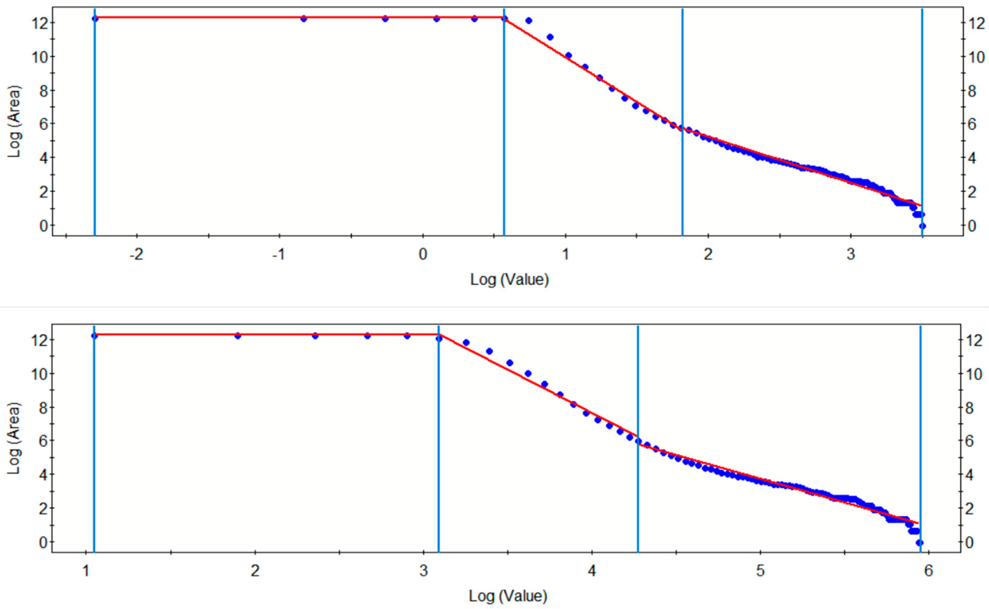
After performing C-A fractal analysis on the IDW interpolation maps of F2 factor scores and Cu element concentrations, the cutoff points were obtained to distinguish between background areas and anomalous areas (Figure 3). The blue line is a segmented line that divides the data into three parts, and the red line is a linear fitting line for the data of different segments. The blue dots represent logA(ρ) (logarithm of the area of anomalies with concentration exceeding the threshold ρ vs. logarithm of ρ). The anomaly zones were classified into weak, moderate, and strong anomaly regions (Figure 4). From the figures, it can be observed that the majority of the area in the F2 factor score map corresponds to weak anomalies after C-A analysis, with the moderate and strong anomaly zones being too limited in extent to serve as reliable indicators for mineral exploration. For the Cu element map, there are 21 known mineral deposits located within the moderate anomaly zones; however, the moderate anomaly area is excessively large, making it difficult to pinpoint potential unknown deposits. Therefore, the Cu element data were further processed by filtering out outliers beyond the range of mean ± 3 standard deviations, followed by generating a new IDW interpolation map and subsequent C-A fractal analysis (Figure 5). Although the anomaly zones became more constrained after this processing, the number of known mineral deposits within the moderate anomaly zone decreased to 14. These results highlight the limitations of raw geochemical data in distinguishing mineralized anomalies from background enrichment. The complex distribution of Cu anomalies suggests that a comprehensive analysis integrating geological settings (e.g., structures, stratigraphy, magmatism) is essential to constrain ore-forming processes and prospecting targets.
Figure 3.
C-A log-log plot of Factor 2 scores (top); C-A log-log plot of Cu (bottom).
Figure 4.
Anomaly zones of Factor 2 scores based on the cutoff points (left: weak anomaly for blue, moderate anomaly for yellow, strong anomaly for red) and Cu element (right: weak anomaly for blue, moderate anomaly for yellow, strong anomaly for red).
Figure 5.
C-A log-log plot of filtered Cu data (outlier removal by mean ± 3 standard deviation) (top) and anomaly distribution (bottom: weak anomaly for blue, moderate anomaly for yellow, strong anomaly for red).
In the northwestern region of Hubei Province, the spatial distribution of copper de-posits is closely associated with fault zones, predominantly exhibiting linear belts along northwest- and northeast-trending faults. Studies indicate that the primary ore-bearing stratigraphic units hosting copper mineralization in this area include the Cryogenian, Ordovician, Cambrian, and Silurian systems. Furthermore, factor analysis has revealed a significant correlation between copper mineralization and elements such as Ag, Zn, Ni, Cu, U, Mo, and Cd. Therefore, this paper uses the MIDW method to interpolate these elements, obtaining their raster maps as evidence layers for FWofE (Figure 6a–g). Based on these characteristics and the spatial relationships among mineral deposits, stratigraphy, and faults, evidence layers can be generated by constructing multi-ring buffer zones around these geological features. Multi-ring buffer zone refers to a series of concentric rings set around key geological features (e.g., faults, ore-bearing strata) to quantify the spatial correlation distance between geological features and mineralization, thereby effectively extracting mineralization-related information. These layers serve as critical inputs for building FWofE models to support mineralization prediction.

Figure 6.
Evidence Layers. (a) Cd geochemical evidence layer, (b) Ag geochemical evidence layer, (c) Cu geochemical evidence layer, (d) Zn geochemical evidence layer, (e) Ni geochemical evidence layer, (f) Mo geochemical evidence layer, (g) U geochemical evidence layer, (h) regional fault evidence layer, (i) Silurian stratigraphic evidence layer, (j) Cryogenian System evidence layer, (k) Ordovician stratigraphic evidence layer, (l) Cambrian stratigraphic evidence layer.
Geological features exhibit significant correlations with mineralization processes within certain spatial extents, which holds important guiding significance for exploration and prospecting. Therefore, to effectively extract mineralization-related information, it is necessary to extend geological elements by appropriate distances to construct evidence layers [61]. Based on this principle, this study designed a multi-ring buffer zone consisting of 10 concentric rings with an interval of 0.5 km each (Figure 6h–l). Statistical analysis shows that this buffer zone encompasses, on average, 85% of the known mineral deposits, while only a very small number of deposits lie outside the buffer range. Consequently, the selected buffer distance and the number of rings can be considered optimal parameters.
To ensure that the geological evidence layers using distance-based buffers are not overly dependent on subjective parameter choices, a small-range perturbation sensitivity analysis was conducted. Following the buffer-distance framework proposed by Zhang et al. [14], which closely matches our study area in scale and sampling density, a baseline distance of 5 km was adopted. We then assessed the robustness of this choice by comparing the C and t statistics derived from buffer distances of 4000 m, 5000 m, and 6000 m (Table A1, Table A2, Table A3, Table A4 and Table A5) [62].
The comparison reveals distinct spatial association patterns that correspond to the geometries observed in the evidence maps. For the regional fault evidence layer (Figure 6h and Table A1): As shown in Figure 6h, the faults form a complex network of structural corridors. Statistically, the contrast values diminish with distance, yet the layer maintains a positive association up to 5000 m (C = 0.05). This 5000 m threshold marks the effective spatial limit of the structural damage zone and fluid migration influence. Beyond this range (at 6000 m), the buffer extends excessively into non-mineralized background areas, causing the correlation to turn negative (C = −0.03), indicating the introduction of regional noise. For the Silurian (Figure 6i) and Cryogenian (Figure 6j) stratigraphic layers: These layers represent the primary ore-hosting horizons (Table A2 and Table 3). While the 4000 m buffer yields the highest raw contrast values due to its tight fit to the outcrop boundaries, the 5000 m buffer retains significant positive associations (e.g., Cryogenian t = 1.54). Visually, Figure 6j shows that the Cryogenian strata are spatially extensive but fragmented; the 5000 m buffer helps bridge the gaps between proximal ore-hosting bodies, accounting for subsurface extensions and geological mapping uncertainties without being overly restricted to fragmented outcrop geometries. For the Ordovician (Figure 6k) and Cambrian (Figure 6l) stratigraphic layers: These act as inhibitory factors. Notably, the Cambrian stratigraphic evidence layer (Figure 6l) displays a stronger negative correlation at 5000 m (C = −0.32) compared to 4000 m (C = −0.22) (Table A5). As seen in Figure 6l, the Cambrian strata form continuous belts that are spatially distinct from known deposits. The wider 5000 m buffer effectively delineates a broader “unfavorable domain,” enhancing the model’s ability to identify unfavorable areas.
Overall, while the 4000 m buffer yields higher contrast values for favorable factors, it risks underestimating the broader spatial influence of negative controls (e.g., Cambrian) and may create fragmented potential zones. The 6000 m buffer clearly introduces considerable regional noise, evidenced by the reversed correlation in faults. Consequently, the 5000 m buffer was selected as the optimal parameter. It provides a robust compromise that captures the maximum effective range of positive structural controls (Faults) while maximizing the identification of unfavorable lithological zones (Cambrian), offering a geologically meaningful representation of the regional metallogenic framework.
Dependence diagnostics for the evidential layers were evaluated using the pairwise Pearson correlation matrix (Table 4). The results show that most correlations fall within the range of −0.30 to 0.35, indicating weak to moderate linear dependence among lithological, structural, and geochemical variables. A few stronger correlations appear among the interpolated geochemical layers (e.g., Cd–Mo, Cd–Cu, and Cu–Ni, with coefficients between 0.60 and 0.79), which is expected because these elements share similar geochemical behavior and partly overlapping mineralization processes. Such moderate correlations are commonly considered acceptable within the framework of the FWofE model, since the method requires conditional independence rather than absolute independence of evidential layers. Therefore, the dependence structure observed in our dataset does not materially violate the conditional-independence assumption of the FWofE model, and the chosen evidential layers can be integrated into the model without producing substantial bias in posterior favourability estimates.
Table 4.
Pairwise correlation matrix of evidential layers.
4.3. Fuzzy Weights-of-Evidence Model
The most critical aspect in constructing a FWofE model is the selection of appropriate evidence layers, which must be closely related to the physicochemical conditions of mineralization. Considering the geological background of northwestern Hubei, the primary ore-hosting stratigraphic units for copper mineralization and regional fault structures were selected as key evidence layers. These geological features exhibit strong spatial associations with the distribution and metallogenic potential of copper deposits, thereby enhancing the model’s capacity to accurately assess the distribution and prospectivity of mineral resources. In addition, geochemical anomalies derived from fluvial sediment data were analyzed to identify elemental patterns associated with copper mineralization. Such geochemical anomalies often serve as indicators of potential mineralized zones. Therefore, incorporating these anomalies as geochemical evidence layers further improves the precision and reliability of the mineral potential assessment [63].
Before constructing the model, it is necessary to define the training and prediction areas in the GeoDAS4.0 software. In most cases, the training area is set to be the same as the prediction area. When delineating the training area, it is important to ensure that the number of grid cells is roughly equivalent to the number of known mineral occurrences. In this study, the spatial unit size of the study area was set to 1,000,000 map units. A total of 24 known copper deposits were selected as the training point layer, and the corresponding number of spatial units was 23.1. This yields a prior probability of 2.91% for the training dataset.
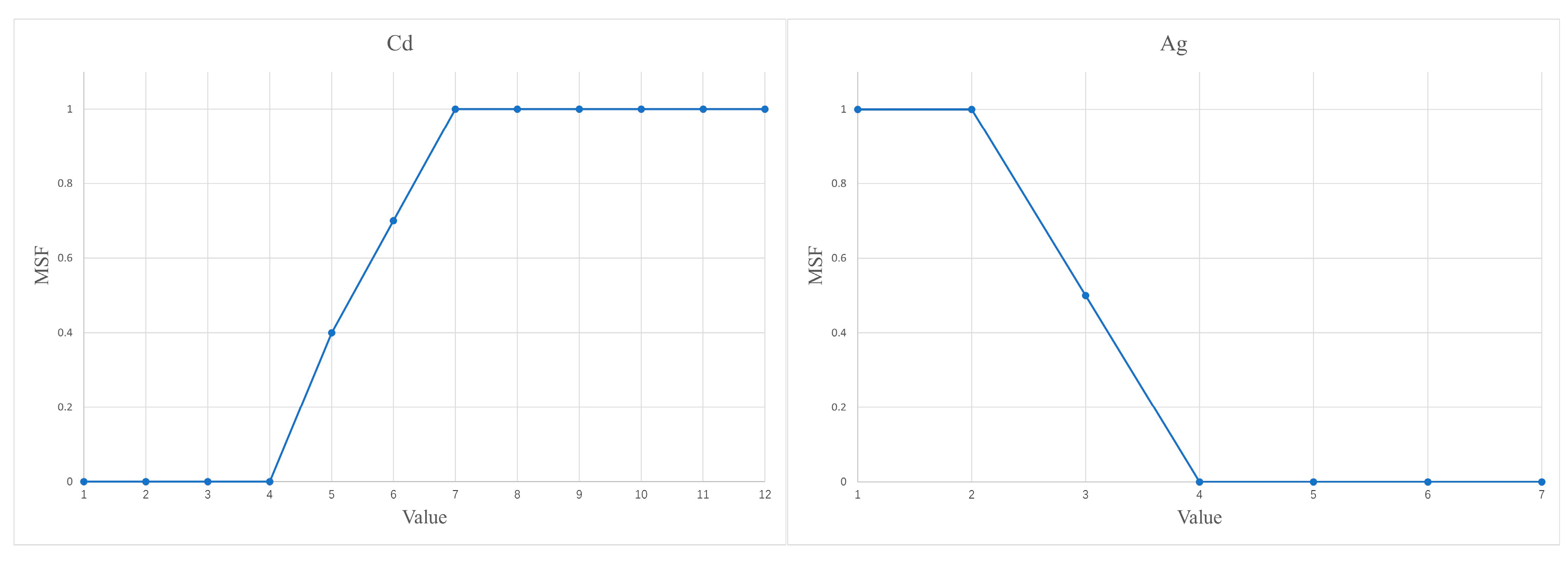
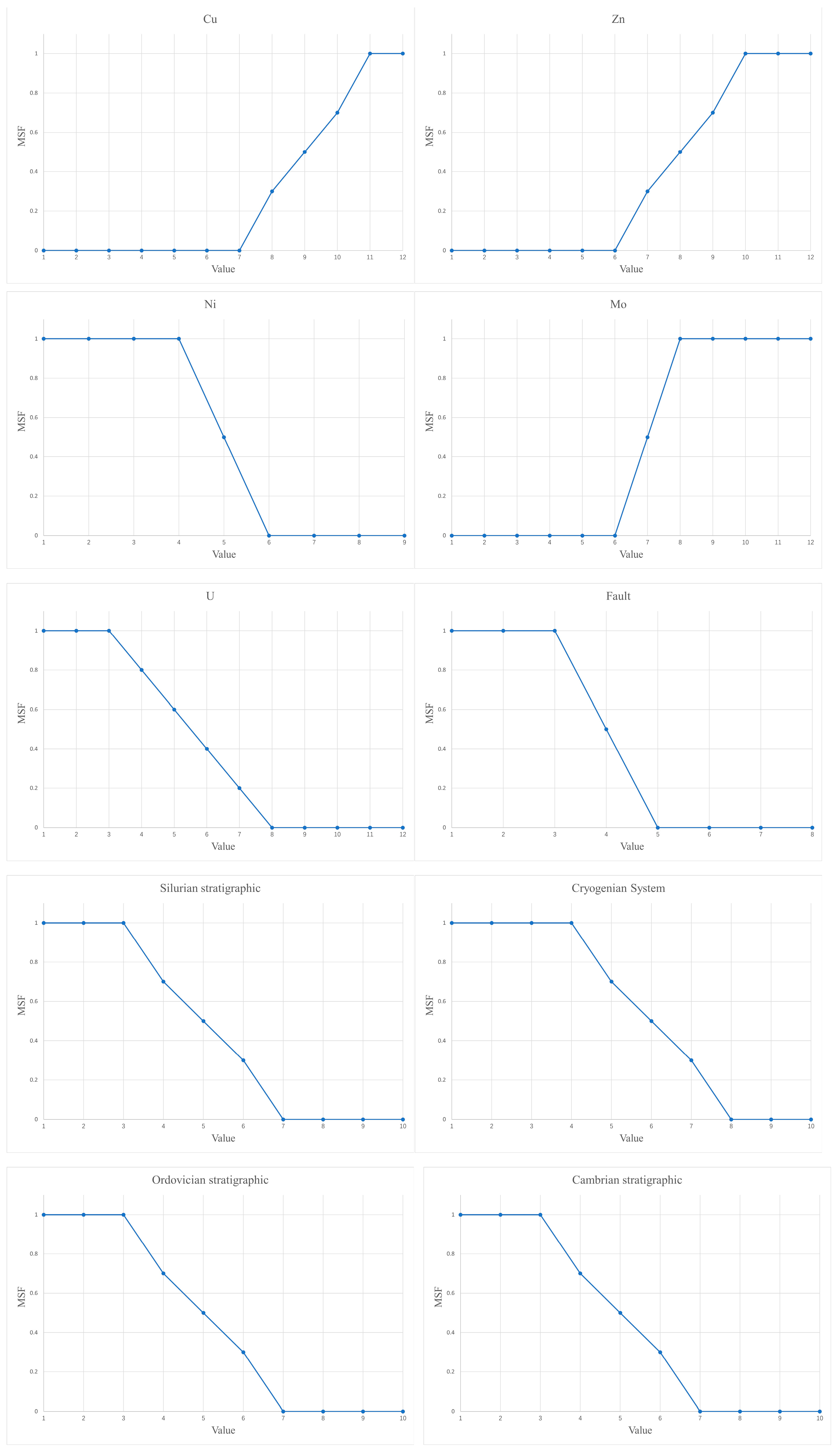
After setting the training parameters, the FWofE for each of the aforementioned evidence layers were calculated. The conventional WofE method determines a binary threshold for each evidence layer based on the maximum value of the ratio t = C/S(C), where C is the contrast (i.e., the difference between positive and negative weights), and S(C) is the standard deviation of the contrast. Areas favorable for mineralization are assigned a value of 1, while unfavorable areas are assigned 0 [64]. In contrast, the FWofE model applies a Membership Standardization Function (MSF) to reclassify the evidence layers. The MSF assigns continuous values within the range [0, 1], reflecting the degree of favorability for mineralization based on the corresponding t-values (Figure 7) [53]. This fuzzy approach allows for a more nuanced representation of mineral potential by incorporating gradational rather than binary classification.
Figure 7.
MSF Classification Evidence Layers (Using Cu and U as Examples).
When calculating FWofE using the GeoDAS4.0 software, the data must be arranged in either cumulative (ascending) or cumulative (descending) order. When cumulative (ascending) order is selected, the first local maximum point from left to right and all points to its left are assigned a value of 1 (Figure 7, U, red), representing an increasing likelihood of mineralization. The relatively high-value points to the right of this maximum are set as fuzzy points and assigned values within the range (0, 1) in sequence (Figure 7, U, yellow), while the remaining points are assigned a value of 0 (Figure 7, U, blue). When cumulative (descending) order is selected, the data are viewed from right to left. The first local maximum point and all points to its right are assigned a value of 1 (Figure 7, Cu, red), the relatively high-value points to the left of this maximum are set as fuzzy points and given values within the range (0, 1) in sequence (Figure 7, Cu, yellow), and all other points are assigned a value of 0 (Figure 7, Cu, blue).
5. Results
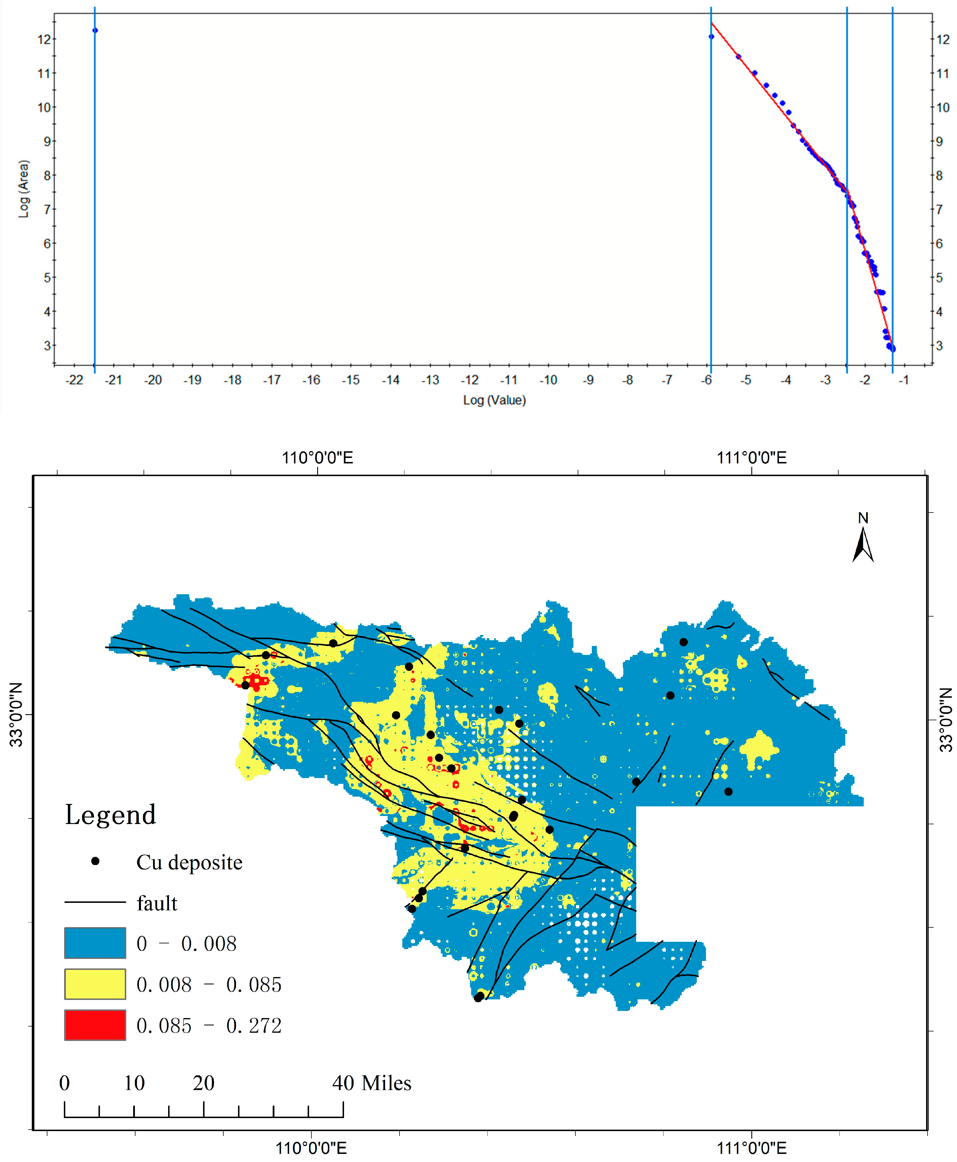
Based on the integrated analysis of 12 evidence layers, a posterior favourability map was generated (Figure 8). After performing C-A fractal analysis, the study area was classified into three levels of mineralization potential (segmentation settings are provided in Table A7). The effectiveness of the FWofE model was evaluated by examining the spatial distribution of known mineral occurrences within the posterior favourability map and applying ROC curve analysis.
Figure 8.
Top: C-A log-log plot of Posterior Favourability for Copper Metallogenic Potential Prediction; Bottom: Posterior Favourability Map of Copper Metallogenic Potential Prediction in Northwestern Hubei Region (weak anomaly for blue, moderate anomaly for yellow, strong anomaly for red).
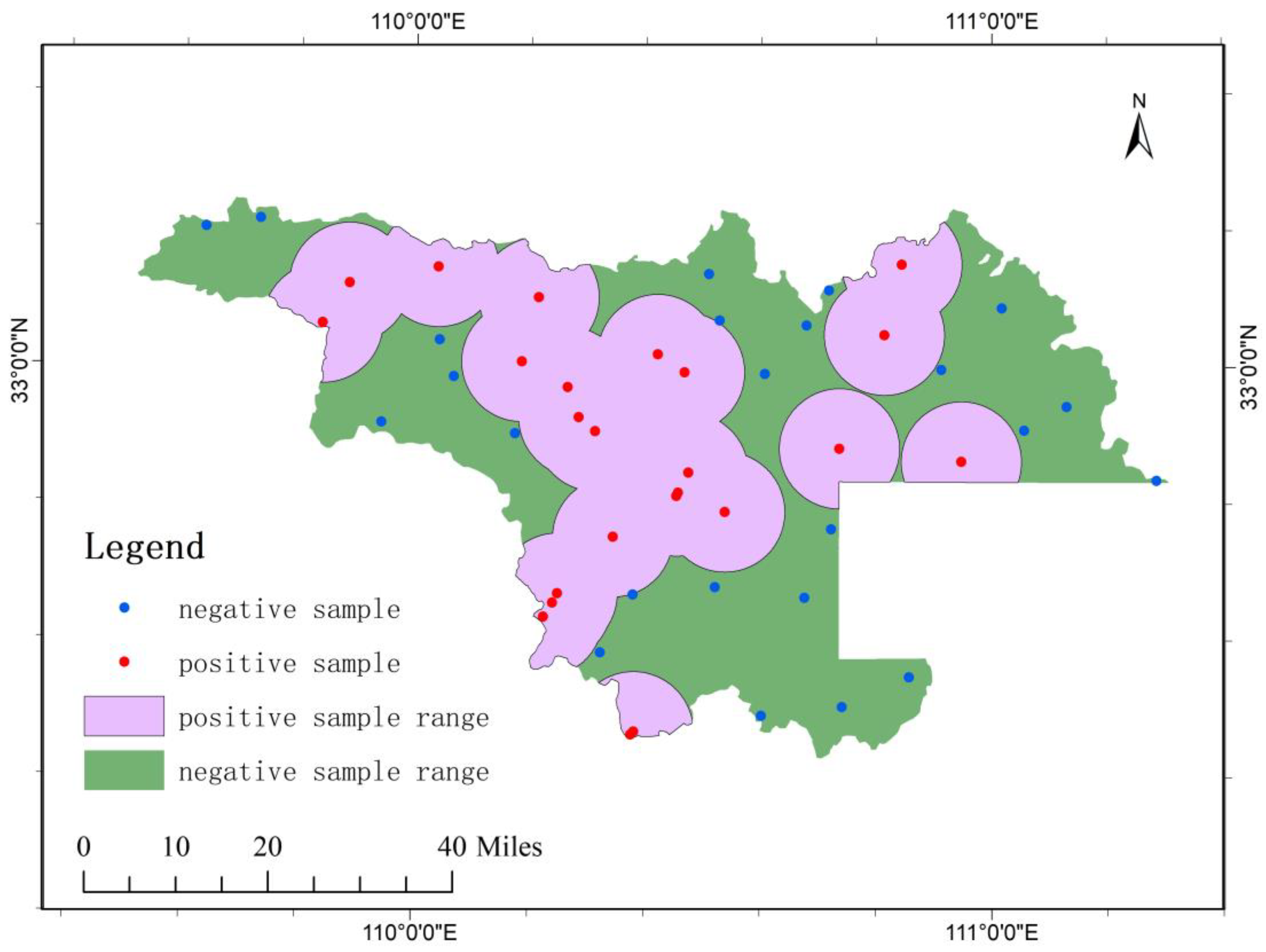
Known copper deposits were designated as positive samples. Circular areas with a radius of 10.5 km centered on these deposits were defined as the positive sample range, representing approximately 50% of the total study area. An equal number of negative samples were randomly selected from outside this range. ROC analysis was then performed for both the fuzzy weights-of-evidence model and the Cu geochemical anomaly map (after outlier filtering), using the same set of positive and negative samples (Figure 9). In the ROC curve analysis, the FWofE model achieved an AUC of 0.844 with a standard error of 0.057 and a 95% confidence interval of 0.733–0.955 (Table 5), while the filtered Cu geochemical anomaly map yielded an AUC of 0.658 (Figure 10).
Figure 9.
Distribution map of positive and negative samples.
Table 5.
Analysis of Area Under the ROC Curve (AUC).
Figure 10.
Predictive Model ROC Curve.
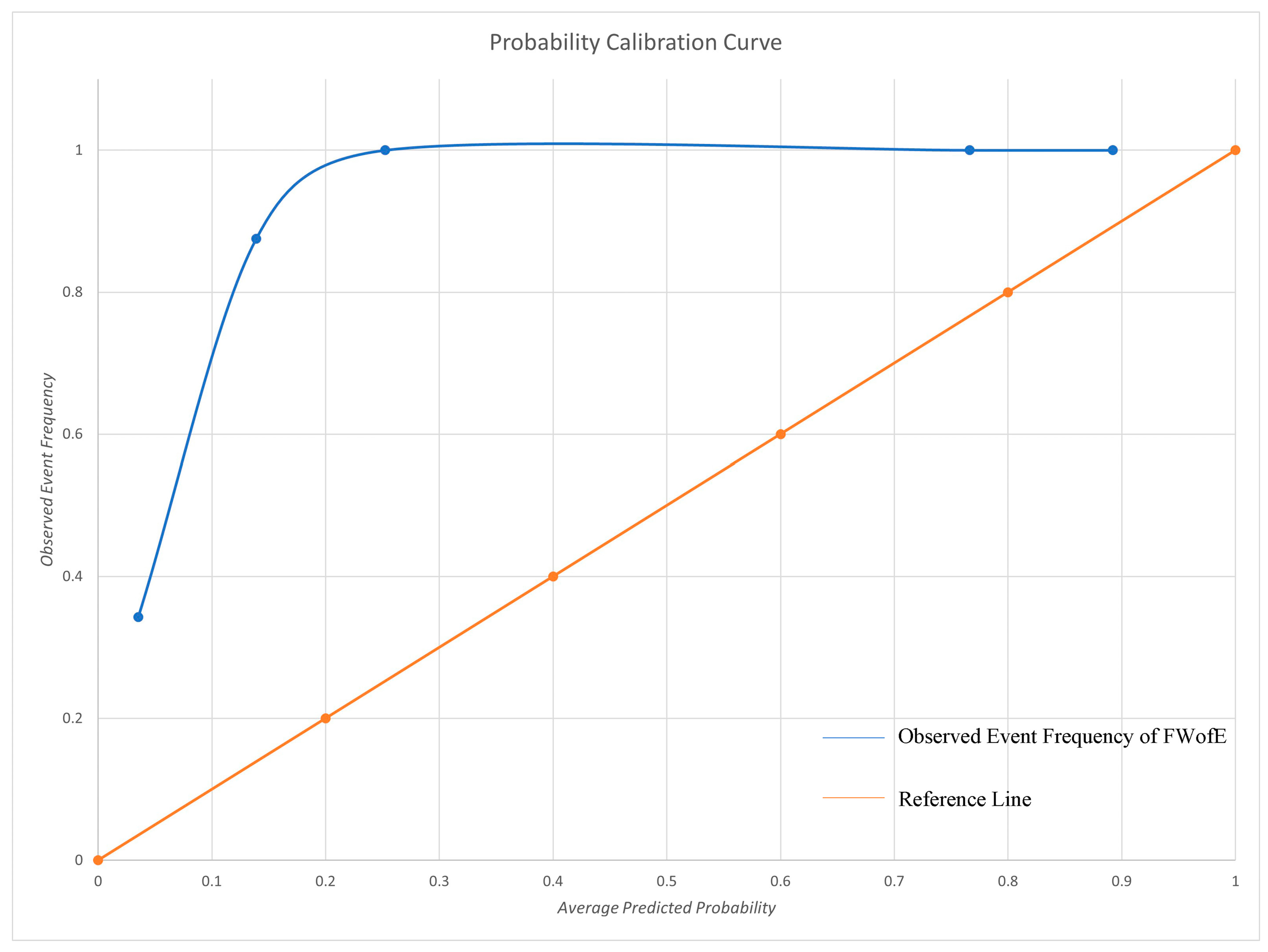
To further evaluate the calibration of the probability outputs, a reliability curve was constructed after normalizing the data (Figure 11). In the low-probability range (0–0.1), the observed event frequency represented by the blue curve are significantly higher than the ideal diagonal, indicating systematically underestimates of true event frequencies and pronounced under-calibration. In the mid-to-high probability interval (0.1–0.8), the blue curve rises rapidly and becomes flatter, showing much closer alignment with the ideal line; the model slightly overestimates the positive probability in this interval, exhibiting mild over-calibration. In the high-probability range (0.8–1.0), the predictions are stable, and the observed positive rate approaches 1, indicating good calibration performance. Overall, the model demonstrates strong discrimination and reasonable calibration in the mid-to-high probability range, although systematic bias remains in the low-probability region. The Brier Score was 0.349, indicating moderate calibration quality [65,66].
Figure 11.
Probability Calibration Curve of the FWofE Model.
By jointly examining the posterior favourability map and the spatial distribution of known copper deposits, potential mineralized areas were delineated. Areas with posterior probabilities in the range of 0.085–0.272 were defined as first level mineral potential zones, containing 5 known deposits. Areas with probabilities ranging from 0.008–0.085 were classified as second level mineral potential zones, containing 14 known deposits. In total, 19 out of 24 known deposits fall within the probability interval of 0.008–0.272, accounting for 79.2% of all known occurrences (Table A8).
The posterior values generated by the FWofE model represent a relative likelihood measure rather than a fully calibrated probability. The observed maximum posterior value of 0.272 reflects the combined effect of fuzzy memberships, evidence weights, and the low prior probability of known deposits. Calibration was assessed using a reliability curve and Brier Score to verify the consistency between predicted scores and actual deposit frequencies.
6. Discussion
The FWofE model constructed in this study was validated by the ROC curve, with an AUC of 0.844, which is significantly higher than the AUC value (0.658) of the single Cu element anomaly map. This proves that the model’s ability to identify copper deposits in the northwestern Hubei region is far superior to that of traditional single-element anomaly extraction methods. In terms of deposit coincidence rate, 19 out of 24 known copper deposits are concentrated in the prospective areas with a posterior favourability ranging from 0.008 to 0.272. Moreover, the spatial overlap rate between the first level prospective areas and known deposits reaches 83%, while that of the second level prospective areas is 75%. These results fully demonstrate that the model can accurately capture the spatial coupling relationship between mineralization and ore-controlling factors, and the prediction results are highly reliable.
The prediction results not only delineate precise prospecting targets but also deepen the understanding of the metallogenic regularity of copper deposits in the study area.
The first level prospective areas are concentrated in the central part of northwestern Hubei, and all overlap with three key elements, namely “NW-trending faults + Cryogenian Yaolinghe Group strata + Factor F2 anomalies”. This confirms the ore-controlling model of “faults as ore-fluid channels, specific strata as ore-hosting carriers, and multi-element synergistic enrichment as metallogenic indicators”.
Although the geochemical anomaly intensity of the second level prospective areas is slightly lower, the matching degree between faults and ore-hosting strata still meets the basic conditions for mineralization. Additionally, some areas with high posterior favourability within these zones (e.g., the central fault intersection zone) have sparse deposit distribution. Combined with the regional tectonic evolution history, these areas are inferred to be undiscovered concealed mineralization areas, filling the gap in traditional prospecting.
Compared with traditional mineral prediction methods, the methodological system of this study has significant innovations:
Comparison with the traditional WofE method: The FWofE model retains the continuous information of evidence layers through a membership function, avoiding data loss caused by binary discretization. This makes the prediction results more consistent with the gradational characteristics of geological bodies.
Comparison with single geochemical anomaly extraction: This study integrates 12 types of evidence layers, including structure, stratigraphy, and multi-element anomalies, overcoming the drawback of traditional methods that “prioritize anomalies while neglecting ore-controlling backgrounds”. It successfully explains the phenomenon that some single-element anomaly areas have no mineralization (e.g., the isolated Cu anomaly area in the east is not classified as a high-prospective area due to the lack of fault channels).
Comparison with ordinary interpolation methods: The MIDW method enhances the identification of weak anomalies, enabling the high-value areas of Factor F2 and Cu elements to more accurately correspond to ore-hosting strata. The coincidence rate between anomaly areas and known deposits is approximately 20% higher than that of ordinary kriging interpolation.
In addition to discrimination ability, probability calibration was also assessed. The reliability curve shows underestimation in low-probability regions and slight overestimation in mid-range intervals, while the Brier Score (0.349) indicates moderate calibration. This highlights the importance of interpreting posterior probabilities as relative indicators of mineralization likelihood rather than precise occurrence probabilities.
However, the spatial configuration in this study introduces limitations. Because the same spatial grid and evidence rasters were used during both model training and evaluation, spatial autocorrelation may lead to inflated AUC estimates. This issue is common in regional-scale mineral prospectivity modeling and should be addressed in future work using spatial block cross-validation or spatial bootstrapping.
This study does not incorporate remote sensing alteration information or deep geophysical data, which may lead to insufficient identification of some mineralization areas controlled by concealed faults. Meanwhile, the weights of evidence layers do not consider differences in metallogenic stages, so the prediction accuracy for multi-stage superimposed mineralization needs to be improved. In the future, high-resolution remote sensing data and magnetotelluric sounding data can be supplemented to optimize the evidence layer system; machine learning algorithms (e.g., random forest) can be integrated to optimize weight allocation, further improving the prospecting prediction accuracy in complex tectonic areas.
7. Conclusions
This study systematically processed 2002 stream sediment samples from northwest-ern Hubei, integrated regional geological, structural, and geochemical data, and applied the FWofE model to assess the copper metallogenic potential. The key conclusions, closely aligned with the research objectives, are as follows:
(1) Factor analysis applied to stream sediment geochemical datasets reveals that Factor F2, comprising Ag, Zn, Ni, Cu, U, Mo, and Cd, functions as a robust indicator of copper mineralization in northwestern Hubei. This elemental assemblage is strongly associated with hydrothermal mineralization processes within the study area. Anomaly maps for Factor F2 and the Cu element, generated through multifractal inverse distance weighting (MIDW) interpolation and C-A fractal modeling, successfully delineate the spatial patterns of mineralization, thereby furnishing high-caliber evidential layers for subsequent metallogenic prospectivity mapping.
(2) The FWofE model, which integrates 12 evidence layers (including 7 geochemical element anomalies, 4 key stratigraphic units, and regional faults), produces a posterior favourability map with strong predictive performance (AUC = 0.844; 95% CI: 0.733–0.955). Among the 24 known copper deposits, 19 (accounting for 79.2%) are distributed within the posterior favourability range of 0.008–0.272, confirming that the model can effectively reflect the spatial coupling relationship between mineralization and ore-controlling factors (stratigraphy and faults). Calibration analysis (Brier Score = 0.349) further indicates that the model offers moderately reliable probability outputs.
(3) The study area is divided into three levels of metallogenic potential zones. The first-level potential zones (with posterior probabilities of 0.085–0.272) are mainly located in the central part of northwestern Hubei, containing 5 known deposits. Notably, most areas within these zones have no reported deposits to date, making them priority targets for future exploration. These target areas show significant spatial association with NW-trending faults and the Cryogenian System, which is consistent with the regional tectono-metallogenic framework.
(4) The methodological framework established in this study, integrating factor analysis, C-A fractal modeling, and FWofE, has proven effective in assessing copper potential in structurally complex regions such as the South Qinling Tectonic Belt. This framework addresses the limitations of traditional binary classification models in handling continuous geochemical variations, providing a replicable methodological reference for mineral resource assessment in regions with similar geological settings.
Author Contributions
Conceptualization, H.S.; Data curation, H.L., H.S. and S.X.; formal analysis, H.S.; funding acquisition, H.L. and X.W.; supervision, H.L. and S.X.; writing—original draft, H.S.; writing—review and editing, S.X. All authors have read and agreed to the published version of the manuscript.
Funding
This research was financially supported by the New geochemical exploration technology for shallow-covered landscapes in desert Gobi and alpine steppes (No. 2024ZD1002400) under the subproject “Geochemical intelligent prospecting prediction and software development for coppernickel and gold deposits” (No. 2024ZD1002406).
Data Availability Statement
The original contributions presented in this study are included in the article. Further inquiries can be directed to the corresponding author.
Acknowledgments
I would like to express my sincere gratitude to Yue Zhou, Weiji Wen, Weihang Zhou, and Xuwei Zhou. I thank Yue Zhou and Weiji Wen for their invaluable guidance, constructive feedback, and continuous support throughout the research process. Meanwhile, I am grateful to Weihang Zhou and Xuwei Zhou for helping me quickly become familiar with the use of software in the early stage of the paper. Special thanks again to Weiji Wen for his guidance and assistance in data collation and manuscript revision. The completion of this research would not have been possible without the collective contributions and collaboration of the entire research team.
Conflicts of Interest
The authors declare no conflicts of interest.
Appendix A

Figure A1.
MSF for evidence. (MSF values assigned to each metallogenic evidence layer in this study. The MSF quantifies the relative importance of individual pieces of evidence in mineral potential prediction; higher MSF values indicate greater contributions to enhancing the posterior favourability.)
Table A1.
C and t Values of the Fault Evidence Layer under Different Buffer Distances.
Table A1.
C and t Values of the Fault Evidence Layer under Different Buffer Distances.
| Distance(m) | C | t | Distance(m) | C | t | Distance(m) | C | t |
|---|---|---|---|---|---|---|---|---|
| 400 | −0.05 | −0.06 | 500 | 0.08 | 0.13 | 600 | 0.1 | 0.17 |
| 800 | 0.24 | 0.48 | 1000 | 0.23 | 0.49 | 1200 | 0.26 | 0.59 |
| 1200 | 0.21 | 0.47 | 1500 | 0.31 | 0.72 | 1800 | 0.24 | 0.58 |
| 1600 | 0.22 | 0.51 | 2000 | 0.25 | 0.59 | 2400 | 0.36 | 0.86 |
| 2000 | 0.22 | 0.53 | 2500 | 0.36 | 0.88 | 3000 | 0.39 | 0.91 |
| 2400 | 0.33 | 0.8 | 3000 | 0.41 | 0.97 | 3600 | 0.19 | 0.46 |
| 2800 | 0.41 | 0.97 | 3500 | 0.24 | 0.56 | 4200 | 0.06 | 0.13 |
| 3200 | 0.36 | 0.84 | 4000 | 0.11 | 0.25 | 4800 | 0.04 | 0.09 |
| 3600 | 0.2 | 0.46 | 4500 | 0.05 | 0.11 | 5400 | 0.02 | 0.04 |
| 4000 | 0.12 | 0.29 | 5000 | 0.05 | 0.11 | 6000 | −0.03 | −0.05 |
Table A2.
C and t Values of the Silurian Evidence Layer under Different Buffer Distances.
Table A2.
C and t Values of the Silurian Evidence Layer under Different Buffer Distances.
| Distance(m) | C | t | Distance(m) | C | t | Distance(m) | C | t |
|---|---|---|---|---|---|---|---|---|
| 400 | 1.33 | 1.56 | 500 | 1.35 | 1.73 | 600 | 1.27 | 1.7 |
| 800 | 1.22 | 1.77 | 1000 | 1.21 | 1.88 | 1200 | 1.06 | 1.66 |
| 1200 | 1.06 | 1.66 | 1500 | 0.89 | 1.39 | 1800 | 0.76 | 1.19 |
| 1600 | 0.84 | 1.32 | 2000 | 0.69 | 1.08 | 2400 | 0.58 | 0.91 |
| 2000 | 0.7 | 1.09 | 2500 | 0.56 | 0.87 | 3000 | 0.45 | 0.7 |
| 2400 | 0.59 | 0.91 | 3000 | 0.45 | 0.7 | 3600 | 0.35 | 0.54 |
| 2800 | 0.49 | 0.77 | 3500 | 0.36 | 0.56 | 4200 | 0.26 | 0.41 |
| 3200 | 0.42 | 0.65 | 4000 | 0.29 | 0.45 | 4800 | 0.19 | 0.29 |
| 3600 | 0.35 | 0.55 | 4500 | 0.22 | 0.35 | 5400 | 0.12 | 0.19 |
| 4000 | 0.29 | 0.46 | 5000 | 0.16 | 0.25 | 6000 | 0.06 | 0.09 |
Table A3.
C and t Values of the Cryogenian Evidence Layer under Different Buffer Distances.
Table A3.
C and t Values of the Cryogenian Evidence Layer under Different Buffer Distances.
| Distance(m) | C | t | Distance(m) | C | t | Distance(m) | C | t |
|---|---|---|---|---|---|---|---|---|
| 400 | 0.58 | 1.13 | 500 | 0.66 | 1.39 | 600 | 0.64 | 1.4 |
| 800 | 0.71 | 1.67 | 1000 | 1.12 | 2.71 | 1200 | 1.25 | 2.96 |
| 1200 | 1.24 | 2.94 | 1500 | 1.48 | 3.25 | 1800 | 1.47 | 3.09 |
| 1600 | 1.49 | 3.22 | 2000 | 1.38 | 2.87 | 2400 | 1.2 | 2.47 |
| 2000 | 1.37 | 2.86 | 2500 | 1.18 | 2.42 | 3000 | 1.13 | 2.21 |
| 2400 | 1.18 | 2.44 | 3000 | 1.13 | 2.2 | 3600 | 1.1 | 2.03 |
| 2800 | 1.11 | 2.22 | 3500 | 1.05 | 1.98 | 4200 | 1.07 | 1.88 |
| 3200 | 1.08 | 2.09 | 4000 | 1.07 | 1.92 | 4800 | 0.92 | 1.62 |
| 3600 | 1.05 | 1.97 | 4500 | 0.99 | 1.75 | 5400 | 0.79 | 1.39 |
| 4000 | 1.09 | 1.94 | 5000 | 0.87 | 1.54 | 6000 | 0.67 | 1.19 |
Table A4.
C and t Values of the Ordovician Evidence Layer under Different Buffer Distances.
Table A4.
C and t Values of the Ordovician Evidence Layer under Different Buffer Distances.
| Distance(m) | C | t | Distance(m) | C | t | Distance(m) | C | t |
|---|---|---|---|---|---|---|---|---|
| 400 | −0.34 | −0.34 | 500 | −0.45 | −0.47 | 600 | −0.34 | −0.4 |
| 800 | −0.29 | −0.39 | 1000 | −0.33 | −0.47 | 1200 | −0.35 | −0.52 |
| 1200 | −0.38 | −0.56 | 1500 | −0.33 | −0.53 | 1800 | −0.32 | −0.55 |
| 1600 | −0.32 | −0.54 | 2000 | −0.28 | −0.51 | 2400 | −0.32 | −0.6 |
| 2000 | −0.32 | −0.57 | 2500 | −0.33 | −0.61 | 3000 | −0.44 | −0.84 |
| 2400 | −0.33 | −0.61 | 3000 | −0.44 | −0.84 | 3600 | −0.56 | −1.07 |
| 2800 | −0.39 | −0.74 | 3500 | −0.58 | −1.09 | 4200 | −0.48 | −0.97 |
| 3200 | −0.49 | −0.94 | 4000 | −0.57 | −1.13 | 4800 | −0.41 | −0.88 |
| 3600 | −0.6 | −1.13 | 4500 | −0.43 | −0.9 | 5400 | −0.4 | −0.88 |
| 4000 | −0.54 | −1.07 | 5000 | −0.4 | −0.86 | 6000 | −0.12 | −0.29 |
Table A5.
C and t Values of the Cambrian Evidence Layer under Different Buffer Distances.
Table A5.
C and t Values of the Cambrian Evidence Layer under Different Buffer Distances.
| Distance(m) | C | t | Distance(m) | C | t | Distance(m) | C | t |
|---|---|---|---|---|---|---|---|---|
| 400 | −0.09 | −0.13 | 500 | 0.12 | 0.21 | 600 | 0.12 | 0.23 |
| 800 | 0.24 | 0.52 | 1000 | 0.33 | 0.73 | 1200 | 0.28 | 0.64 |
| 1200 | 0.34 | 0.79 | 1500 | 0.28 | 0.66 | 1800 | 0.24 | 0.57 |
| 1600 | 0.29 | 0.69 | 2000 | 0.26 | 0.64 | 2400 | 0.13 | 0.32 |
| 2000 | 0.22 | 0.54 | 2500 | 0.14 | 0.34 | 3000 | 0.04 | 0.1 |
| 2400 | 0.15 | 0.37 | 3000 | 0.04 | 0.1 | 3600 | −0.13 | −0.31 |
| 2800 | 0.09 | 0.21 | 3500 | −0.1 | −0.24 | 4200 | −0.27 | −0.64 |
| 3200 | −0.02 | −0.04 | 4000 | −0.22 | −0.53 | 4800 | −0.34 | −0.82 |
| 3600 | −0.13 | −0.31 | 4500 | −0.32 | −0.78 | 5400 | −0.23 | −0.55 |
| 4000 | −0.22 | −0.54 | 5000 | −0.32 | −0.78 | 6000 | −0.19 | −0.45 |
Note: Table A1, Table A2, Table A3, Table A4 and Table A5 summarize the C and t values calculated for the faults, Silurian, Cryogenian, Ordovician, and Cambrian evidence layers under buffer distances of 4000 m, 5000 m, and 6000 m. These statistics are used solely to determine the optimal buffer distance for each evidence layer and are not exactly the same as the data used for assigning the MSF values.
Table A6.
Parameter settings used in GeoDAS4.0 for spatial data processing.
Table A6.
Parameter settings used in GeoDAS4.0 for spatial data processing.
| Parameter Category | Parameter | Value | Note |
|---|---|---|---|
| General Settings | Neighbourhood size | 7 | Default GeoDAS4.0 setting |
| Search radius | 38,477.0 m | Default GeoDAS4.0 setting | |
| Singularity exponent | 1 | Default GeoDAS4.0 setting | |
| C-A Segmentation | C-A segmentation settings | See Table A6 | GeoDAS4.0 Software default segmentation scheme |
| Coordinate System | Coordinate reference system | CGCS2000_3_Degree_GK_CM_111E | CRS used for all datasets |
| Grid Resolution | Geochemical elements | 192.4 m | Resolution after rasterization |
| Fault layer | 370.7 m | – | |
| Silurian strata | 95.3 m | – | |
| Other stratigraphic layers | 141.8 m | Cambrian, Ordovician, Cryogenian |
Note: In this study, fuzzy membership thresholds were not manually set; instead, the default evidential weighting workflow in GeoDAS4.0 was used. In this workflow, the fuzzy membership thresholds are automatically assigned based on the data range of each evidence layer. Under this default mode, GeoDAS4.0 sets the minimum value of the data as the lower threshold (a) and the maximum value as the upper threshold (b), using a linear membership function for calculation. Since these parameters are automatically generated by the GeoDAS4.0 software and were not manually modified, their specific values are not displayed in the interface.
Table A7.
Segmentation Parameters of C-A Fractal Analysis for Mineralization Favourability.
Table A7.
Segmentation Parameters of C-A Fractal Analysis for Mineralization Favourability.
| Value | A | B | Errors |
|---|---|---|---|
| 4.62 × 10⁻¹⁰ | 0 | 0 | 0 |
| 0.0027−0.085 | 3.906853 | −1.45319 | 1.44 × 10⁻² |
| 0.085−0.266 | −2.31175 | −4.0349 | 0.064178 |
Note: In this table, “Value” denotes the intervals of mineralization favourability, “A” represents the intercept of the C-A fractal model, “B” is the slope, and “Errors” indicates the model fitting error.
Table A8.
C-A Threshold Intervals, Mapped Area, and Deposit Counts.
Table A8.
C-A Threshold Intervals, Mapped Area, and Deposit Counts.
| C-A Break Values | Area/m2 | Deposits |
|---|---|---|
| 0–0.008 | 6023576000 | 5 |
| 0.008–0.085 | 1842008000 | 14 |
| 0.085–0.272 | 60292380 | 5 |
Note: provides the C-A threshold intervals extracted from the Posterior Favourability Map of copper metallogenic potential prediction in the northwestern Hubei region, it also reports the mapped area and number of known deposits within each threshold range. Because the area is calculated based on raster cell counts, the total area will be slightly smaller than the actual study area.
References
- Zhang, N. Supply and demand situation of China’s copper industry in 2023. China Min. Mag. 2024, 33, 20–28. (In Chinese) [Google Scholar] [CrossRef]
- Tang, J.; Yang, H.; Chen, H.; Li, F.; Wang, C.; Liu, Q.; Zhang, Q.; Zhang, R.; Yu, L. Potential and future direction for copper resource exploration in China. Green Smart Min. Eng. 2024, 1, 127–131. [Google Scholar] [CrossRef]
- Liang, S.; Lyu, X. Research on the evolution of supply and consumption patterns of copper resources around the world and the influencing factors of copper consumption in China. China Min. Mag. 2025, 34, 324–332. [Google Scholar] [CrossRef]
- Chen, L.; Tang, L.; Shen, Y.; Guo, X.; Zhao, F.; Sheng, Y.; Zeng, T.; Wang, H.; Chen, Y. Comparison on Metallogenic Differences of Porphyry Deposits between Luanchuan Mo-W and Zhashui-Shanyang Cu-Mo Ore-clusters in Qinling Orogenic Belt: Constraints of Magmatic Source and Metallogenic Conditions. Northwestern Geol. 2024, 57, 67–89. [Google Scholar] [CrossRef]
- Dai, S.; Xue, Y. Tectonic development and evolution of the eastern segment of the Qinling Orogenic Belt and its relationship with gold, silver, and copper mineralization. China’s Manganese Ind. 2018, 36, 69–71+82. (In Chinese) [Google Scholar] [CrossRef]
- Yao, S.; Ding, Z.; Zhou, Z.; Chen, S. Metallic metallogenic systems of the Qinling Orogenic Belt. Earth Sci. 2002, 27, 599–604. (In Chinese) [Google Scholar]
- Chen, G.; Shu, L.; Shu, L.; Zhang, C.; Ouyang, Y. Geological characteristics and mineralization setting of the Zhuxi tungsten (copper) polymetallic deposit in the Eastern Jiangnan Orogen. Sci. China Earth Sci. 2016, 59, 803–823. [Google Scholar] [CrossRef]
- Chen, G.; Shu, L.; Shu, L.; Zhang, C.; Ouyang, Y. Contributions of juvenile lower crust and mantle components to porphyry Cu deposits in an intracontinental setting: Evidence from late Mesozoic porphyry Cu deposits in the South Qinling Orogenic Belt, Central China. Min. Depos. 2023, 58, 489–509. [Google Scholar] [CrossRef]
- Yu, X.; Li, J.; Jin, X.; Zhao, S.; He, C.; Zhu, Y. Monazite U-Th-Pb and sericite Rb-Sr dating of the Xiajiadian gold deposit hosted in black shales in the Qinling Orogenic Belt and their implications for regional gold mineralization. Sci. China Earth Sci. 2024, 54, 2515–2533. [Google Scholar] [CrossRef]
- Ouyang, Y.; Liu, H.; Li, G.; Ma, D.; Zhang, L.; Huang, H.; Zhang, J.; Zhang, T.; Liu, B.; Zhao, Y.; et al. Mineral search prediction based on Random Forest algorithm—A case study on porphyry-epithermal copper polymetallic deposits in the western Gangdise meatallogenic belt. Geol. China 2023, 50, 303–330. [Google Scholar] [CrossRef]
- Ford, A. Practical Implementation of Random Forest-Based Mineral Potential Mapping for Porphyry Cu–Au Mineralization in the Eastern Lachlan Orogen, NSW, Australia. Nat. Resour. Res. 2020, 29, 267–283. [Google Scholar] [CrossRef]
- Cheng, Q.M. A New Model for Quantifying Anisotropic Scale Invariance and for Decomposition of Mixing Patterns. Math. Geol. 2004, 36, 345–360. [Google Scholar] [CrossRef]
- Li, J.; Xie, S.; Yang, W.; Zhou, W.; Carranza, E.J.M.; Wen, W.; Shi, H. Prediction of Selenium-Enriched Crop Zones in Xiaoyan Town Using Fuzzy Logic and Machine Learning Approaches. Appl. Sci. 2025, 15, 4943. [Google Scholar] [CrossRef]
- Zhang, Y.; Ye, X.; Xie, S.; Dong, J.; Yaisamut, O.; Zhou, X.; Zhou, X. Prediction of Au-Polymetallic Deposits Based on Spatial Multi-Layer Information Fusion by Random Forest Model in the Central Kunlun Area of Xinjiang, China. Minerals 2023, 13, 1302. [Google Scholar] [CrossRef]
- Behera, S.; Panigrahi, M.K. Gold prospectivity mapping and exploration targeting in Hutti-Maski schist belt, India: Synergistic application of Weights-of-Evidence (WOE), Fuzzy Logic (FL) and hybrid (WOE-FL) models. J. Geochem. Explor. 2022, 235, 0375–6742. [Google Scholar] [CrossRef]
- Maysam, A.; Gholam-Hossain, N. Integration of various geophysical data with geological and geochemical data to determine additional drilling for copper exploration. J. Appl. Geophys. 2012, 83, 35–45. [Google Scholar] [CrossRef]
- Zhang, J.; Chen, H.; Ren, J.; Wei, Z.; Sun, K.; Hu, P.; Wu, D.; Gu, A.; Sun, H.; Zuo, L.; et al. Mineral Resource Assessment Methods Comparison and Its Development Trend Discussion. Northwestern Geol. 2023, 56, 292–305. [Google Scholar] [CrossRef]
- Li, H.; Lu, S.; Chen, Z.; Xiang, Z.; Zhou, H.; Hao, G. Zircon U-Pb geochronology of rift-type volcanic rocks of the Yaolinghe Group in the South Qinling orogen. Geol. Bull. China 2003, 22, 775–781. [Google Scholar]
- Guo, Q.; Zhang, J.; Mao, X.; Wu, Y. Genetic mechanism of Cambrian plagiogranites in the Shangdan Suture Zone, West Qinling: Implications for the initiation of Paleo-Tethys Ocean subduction. Acta Petrol. Mineral. 2024, 43, 304–329. [Google Scholar] [CrossRef]
- Yue, S.W.; Deng, X.H. Geological and Ore-Forming Characteristics of Ag-Au and Polymetallic Deposits in Northwestern Hubei, China. Earth Sci. Front. 2019, 26, 106–128. (In Chinese) [Google Scholar] [CrossRef]
- Lin, S.; Li, Y.; Wang, W.; Liao, W.; Qiao, Y. Study on Geological and Geophysical Features of Yunxian Basin Segment of Liangyun Fault Belt. J. Geod. Geodyn. 2019, 39, 148–152. [Google Scholar] [CrossRef]
- Yang, J.; Xiao, Y.; Shi, Z.; Sun, H. Geological Characteristics and Prospecting Potential of Ultra-poor Magnetite in the Yaolinghe Formation, Northwestern Hubei. Resour. Environ. Eng. 2010, 24, 122–129+157. [Google Scholar] [CrossRef]
- Zhang, Q. Sedimentary characteristics, provenance analysis and tectonic setting of the Yangping Formation of the Wudang Group in northwestern Hubei. Master’s Thesis, China University of Geosciences, Beijing, China, 2020. [Google Scholar] [CrossRef]
- Ling, W.; Duan, R.; Liu, X.; Cheng, J.; Mao, X.; Peng, L.; Liu, Z.; Yang, H.; Ren, B. U-Pb Dating of Detrital Zircons from the Wudangshan Group in the South Qinling and Its Geological Significance. Chin. Sci. Bull. 2010, 55, 1153–1161. (In Chinese) [Google Scholar] [CrossRef]
- Xu, T.; Ma, C.; Lu, X.; Liu, X. Geological Characteristics and Prospecting Direction of Shejiayuan Silver-Gold Deposit in Yunxi County, Hubei Province. Resour. Environ. Eng. 2012, 26, 104–110. [Google Scholar] [CrossRef]
- Dong, Q.; Chen, J.; Tang, Y. Application of R type factor analyses in mineralization prognosis: By an example of Huangbuling gold deposit, Shandong province. Geol. Explor. 2008, 44, 64–68. (In Chinese) [Google Scholar]
- Wang, H.; Chen, S. Factor analysis-based extraction and evaluation of anomaly information—A case study of the Nanyang Basin and orogenic belt. Contrib. Geol. Miner. Resour. Res. 2021, 36, 105–113. (In Chinese) [Google Scholar] [CrossRef]
- Zhu, P. Application of Factor and Singularity-Quantile Analyses for Gold Potential Mapping Based on Geochemical Data in the Biguo Area, Shandong Province, China. Arab. J. Geosci. 2022, 15, 1617. [Google Scholar] [CrossRef]
- Zuo, R.G.; Carranza, E.J.M.; Cheng, Q.M. Fractal/Multifractal Modelling of Geochemical Exploration Data. J. Geochem. Explor. 2012, 122, 1–3. [Google Scholar] [CrossRef]
- Hassanpour, S.; Afzal, P. Application of Concentration–Number (C–N) Multifractal Modeling for Geochemical Anomaly Separation in Haftcheshmeh Porphyry System, NW Iran. Arab. J. Geosci. 2013, 6, 957–970. [Google Scholar] [CrossRef]
- Zhang, Y.; Ye, X.; Xie, S.; Zhou, X.; Awadelseid, S.F.; Yaisamut, O.; Meng, F. Implication of multifractal analysis for quantitative evaluation of mineral resources in the Central Kunlun area, Xinjiang, China. Geochem. Explor. Environ. Anal. 2022, 22, geochem2021-083. [Google Scholar] [CrossRef]
- Greenacre, M.; Groenen, P.J.F.; Hastie, T.; D’eNza, A.I.; Markos, A.; Tuzhilina, E. Principal component analysis. Nat. Rev. Methods Primers 2022, 2, 100. [Google Scholar] [CrossRef]
- Deng, Y.; Zhang, J.; Zhong, R.; He, X.; Wang, X. Application of machine learning-based principal component analysis in the discrimination of gold deposit types: A case study of geochemical characteristics of pyrite elements. Acta Petrol. Sin. 2024, 40, 1801–1816. [Google Scholar] [CrossRef]
- Cheng, Q.M. GeoData Analysis System (GeoDAS) for Mineral Exploration: User’s Guide and Exercise Manual; Material for the Training Workshop on GeoDAS Held at York University: Toronto, ON, Canada, 2000. [Google Scholar]
- Cheng, Q.M. Multifractal and geostatistic methods for characterizing local structure and singularity properties of exploration geochemical anomalies. Earth Sci. 2001, 26, 161–166. [Google Scholar]
- Yan, L. Research on surface elevation interpolation method based on multifractal theory. Sci. Technol. Inf. 2013, 35, 36–38. [Google Scholar] [CrossRef]
- Parsa, M.; Maghsoudi, A.; Yousefi, M.; Carranza, E.J.M. Multifractal Interpolation and Spectrum—Area Fractal Modeling of Stream Sediment Geochemical Data: Implications for Mapping Exploration Targets. J. Afr. Earth Sci. 2017, 128, 5–15. [Google Scholar] [CrossRef]
- Cheng, Q.M. Modeling Local Scaling Properties for Multiscale Mapping. Vadose Zone J. 2008, 7, 525–532. [Google Scholar] [CrossRef]
- Cheng, Q.M. Multifractal Interpolation Method for Spatial Data with Singularities. J. S. Afr. Inst. Min. Metall. 2015, 115, 235–240. [Google Scholar] [CrossRef]
- Wen, W.; Yang, F.; Xie, S.; Wang, C.; Song, Y.; Zhang, Y.; Zhou, W. Determination of Geochemical Background and Baseline and Research on Geochemical Zoning in the Desert and Sandy Areas of China. Appl. Sci. 2024, 14, 10612. [Google Scholar] [CrossRef]
- Cheng, Q.M.; Agterberg, F.P.; Ballantyne, S.B. The Separation of Geochemical Anomalies from Background by Fractal Methods. J. Geochem. Explor. 1994, 51, 109–130. [Google Scholar] [CrossRef]
- Zuo, R.G.; Xia, Q.L.; Zhang, D.J. A Comparison Study of the C–A and S–A Models with Singularity Analysis to Identify Geochemical Anomalies in Covered Areas. Appl. Geochem. 2013, 33, 165–172. [Google Scholar] [CrossRef]
- Rock, N.M. Statistical Applications in the Earth Sciences: By Frits P. Agterberg and Graeme F. Bonham-Carter, editors, 1990, Geological Survey of Canada Paper 89-9, 588 p., $50 (Canadian) approximately. Comput. Geosci. 1991, 17, 474–475. [Google Scholar] [CrossRef]
- Cheng, Q.M.; Zhang, S.Y. Fuzzy Weights of Evidence Method Implemented in GeoDAS GIS for Information Extraction and Integration for Prediction of Point Events. Tor. Int. Geosci. Remote Sens. Symp. 2002, 5, 2933–2935. [Google Scholar] [CrossRef]
- Hong, H.; Ilia, I.; Tsangaratos, P.; Chen, W.; Xu, C. A hybrid fuzzy weight of evidence method in landslide susceptibility analysis on the Wuyuan area, China. Geomorphology 2017, 290, 1–16. [Google Scholar] [CrossRef]
- Ali, K.; Cheng, Q.; Li, W.; Chen, Y. Multi-Element Association Analysis of Stream Sediment Geochemistry Data for Predicting Gold Deposits in South-Central Yunnan Province, China. Geochem. Explor. Environ. Anal. 2006, 6, 341–348. [Google Scholar] [CrossRef] [PubMed]
- Wang, J.; Zeng, W.; Zhang, Q.; Chen, J.; Teng, F.; Li, W.; Liu, X. Application of fuzzy weights of evidence method in metallogenic prediction for alaskite-type uranium deposits in Namibia. Geol. Bull. China 2023, 42, 1318–1333. [Google Scholar] [CrossRef]
- Agterberg, F.P.; Bonharn-Carter, G.F. Weights of Evidence Modeling and Weighted Logistic Regression for Mineral Potential Mapping; Oxford University Press: New York, NY, USA, 1994. [Google Scholar] [CrossRef]
- Cheng, Q.M.; Agterberg, F.P. Fuzzy Weights of Evidence Method and Its Application in Mineral Potential Mapping. Nat. Resour. Res. 1999, 8, 27–35. [Google Scholar] [CrossRef]
- Xie, S.; Wan, X.; Dong, J.; Wan, N.; Jiang, X.; Carranza, E.J.M.; Wang, X.; Chang, L.; Tian, Y. Quantitative prediction of potential areas likely to yield Se-rich and Cd-low rice using fuzzy weights-of-evidence method. Sci. Total Environ. 2023, 889, 164015. [Google Scholar] [CrossRef]
- Xie, S.; Huang, N.; Deng, J.; Wu, S.; Zhan, M.; Carranza, E.J.M.; Zhang, Y.; Meng, F. Quantitative prediction of prospectivity for Pb–Zn deposits in Guangxi (China) by back-propagation neural network and fuzzy weights-of-evidence modelling. Geochem. Explor. Environ. Anal. 2022, 22, geochem2021-085. [Google Scholar] [CrossRef]
- Huo, Y.; Wang, Y.; Wu, Q.; Wang, Z.; Wang, X.; Liu, D.; Li, Z. Analysis method of gold reserve mineral deposit in Yunnan Province based on fuzzy evidence weight. Prog. Geophys. 2022, 37, 2552–2561. (In Chinese) [Google Scholar] [CrossRef]
- Deng, J.; Zhan, M.; Zhou, W.; Wu, S.; Huang, N.; Zhang, R.; Xie, S. Quantitative prediction of mineral resources in typical gold deposits in Guangxi, China using a fuzzy weights of evidence method. Chin. J. Geomech. 2021, 27, 374–390. [Google Scholar] [CrossRef]
- Porwal, A.; Carranza, E.J.M.; Hale, M. Artificial neural networks for mineral-potential mapping: A case study from Aravalli Province, Western India. Nat. Resour. Res. 2003, 12, 155–171. [Google Scholar] [CrossRef]
- Xiao, K.Y.; Zhang, X.H.; Chen, Z.H. Comparison of Evidence Weight Method and Information Method in Metallogenic Prediction. Comput. Tech. Geophys. Geochem. Explor. 1999, 21, 223–226. [Google Scholar]
- Zhou, G. Machine Learning-Based Mineralization Prediction of Sn-Cu Polymetallic Deposits in the Gejiu Area. Master’s Thesis, China University of Geosciences, Beijing, China, 2021. [Google Scholar] [CrossRef]
- Gao, Y.; Zhang, Z.J.; Xiong, Y.H. Mapping Mineral Prospectivity for Cu Polymetallic Mineralization in Southwest Fujian Province, China. Ore Geol. Rev. 2016, 75, 16–28. [Google Scholar] [CrossRef]
- Egan, J.P. Signal Detection Theory and ROC Analysis; In Series in Cognition and Perception; Academic Press: New York, NY, USA, 1975. [Google Scholar]
- Parsa, M.; Maghsoudi, A.; Yousefi, M. A Receiver Operating Characteristics-Based Geochemical Data Fusion Technique for Targeting Undiscovered Mineral Deposits. Nat. Resour. Res. 2018, 27, 15–28. [Google Scholar] [CrossRef]
- Shalabi, L.A.; Shaaban, Z.; Kasasbeh, B. Data Mining: A Preprocessing Engine. J. Comput. Sci. 2006, 2, 735–739. [Google Scholar] [CrossRef]
- Carranza, E.J.M.; Hale, M. Geologically Constrained Probabilistic Mapping of Gold Potential, Baguio District, Philippines. Nat. Resour. Res. 2000, 9, 237–253. [Google Scholar] [CrossRef]
- Zhang, Z.; Zuo, R.; Xiong, Y. A Comparative Study of Fuzzy Weights of Evidence and Random Forests for Mapping Mineral Prospectivity for Skarn-Type Fe Deposits in the Southwestern Fujian Metallogenic Belt, China. Sci. China Earth Sci. 2016, 59, 556–572. [Google Scholar] [CrossRef]
- Lin, Y.; Wang, L.; Ouyang, Y.; Li, Z.; Zeng, R.; Chen, Q.; Deng, Y. Evaluation of Copper Mineral Resource Potential Using Concentration–Area Fractal Model and Fuzzy Evidence Weighting: A Case Study of the Jiurui Region in Jiangxi. Northwestern Geol. 2024, 57, 165–178. [Google Scholar] [CrossRef]
- Huang, X.; Li, H.; Li, Z.; Zeng, H.; Guo, F.; Wu, Z.; Deng, T.; Liu, J. Application of fuzzy weights of evidence method to prediction of mineralization in the volcanic-type uranium deposit in Xiangshan basin, Jiangxi. World Nucl. Geol. 2023, 40, 226–235. [Google Scholar] [CrossRef]
- Murphy, A.H. A New Vector Partition of the Probability Score. J. Appl. Meteorol. 1973, 12, 595–600. [Google Scholar] [CrossRef]
- Guo, C.; Pleiss, G.; Sun, Y.; Weinberger, K.Q. On calibration of modern neural networks. In Proceedings of the 34th International Conference on Machine Learning, Sydney, NSW, Australia, 6–11 August 2017; pp. 1321–1330. [Google Scholar]
Disclaimer/Publisher’s Note: The statements, opinions and data contained in all publications are solely those of the individual author(s) and contributor(s) and not of MDPI and/or the editor(s). MDPI and/or the editor(s) disclaim responsibility for any injury to people or property resulting from any ideas, methods, instructions or products referred to in the content. |
© 2025 by the authors. Licensee MDPI, Basel, Switzerland. This article is an open access article distributed under the terms and conditions of the Creative Commons Attribution (CC BY) license (https://creativecommons.org/licenses/by/4.0/).