Integrating Geological Domains into Machine Learning for Ore Grade Prediction: A Case Study from a Porphyry Copper Deposit

Abstract

Accurate grade prediction in porphyry copper deposits requires not only capturing spatial continuity but also accounting for geological controls. This study evaluates the added value of incorporating alteration and mineralization domains into machine learning (ML) models for copper grade estimation at the Iju porphyry Cu deposit, Iran. We compare four scenarios: spatial coordinates only, coordinates + alteration, coordinates + mineralization, and coordinates + both domains. A three-stage workflow was developed, in which Random Forest classifiers—optimized with Particle Swarm Optimization (PSO-RF)—classify alteration and mineralization zones, which are later integrated into regression models for ore grade prediction. Model performance was assessed using nested spatial cross-validation and benchmarked against Support Vector Machines (SVM). In comparative analysis, the PSO-RF framework consistently outperformed SVM, achieving more balanced accuracy between training and testing data and demonstrating greater robustness to class imbalance in domain classification. Moreover, results show that combining alteration and mineralization domains improves predictive performance (R² = 0.78; RMSE was reduced by 5.6% relative to coordinates-only). Although numerically moderate, this reduction in error translates into more reliable tonnage and grade estimations near cut-off grades, thereby enhancing the economic confidence of resource evaluations. These findings demonstrate that integrating multiple geological domains can improve both the accuracy and interpretability of ML-based grade models, providing a practical and reproducible workflow for porphyry copper resource evaluation.

1. Introduction

Mineral resource estimation is a fundamental step of any mining project, as it provides the essential basis for mine planning, economic evaluation, investment decision-making, and risk assessment. Accurate and reliable estimation of both tonnage and grade is critical to the viability of a mining operation, since inaccuracies can lead to significant financial and technical consequences [1,2]. Traditionally, geostatistical methods (kriging or conditional simulation) have been widely used for mineral resource estimation [3,4]. However, despite their significant advantages, challenges remain regarding parameter inference and distributional assumptions. Additionally, mineral grades often exhibit complex spatial structures and heterogeneity [5,6]. The accuracy of geostatistical approaches depends on effectively identifying and capturing these complex spatial and multivariate structures, which can be a cumbersome task [7,8,9]. The process of constructing and updating geostatistical models can also be computationally intensive and time-consuming, particularly in the presence of large or frequently updated datasets [8]. One promising solution to overcome these challenges is the use of machine learning (ML) techniques, with numerous studies demonstrating their efficacy in mineral resource estimation [10,11,12,13,14,15]. ML techniques excel in handling non-linear and complex relationships in data, without distributional assumptions and with fewer parameters to be determined, thereby simplifying the inference process. These advantages make ML methods a valuable alternative for estimation of mineral grade, and in recent years, these methods have emerged as a promising alternative or complement to geostatistical approaches [16,17,18]. Over the last decade, a wide range of ML models have been applied to mineral grade estimation across different types of mineral deposits. Among the most commonly implemented approaches are Artificial Neural Networks (ANNs), Support Vector Machines (SVMs), Random Forests (RFs), and Gaussian Processes (GPs) [2,11,13,19,20,21]. These algorithms have demonstrated considerable potential in the estimation of mineral resources, often leading to improved prediction accuracy compared to conventional geostatistical methods.

In most ML-based studies on ore grade estimation, predictive models have primarily relied on spatial coordinates as the main input variables, enabling the models to learn the relationship between sample location and observed grade values [2]. While this spatially driven approach can be effective in certain geological settings, it inherently limits the model’s capacity to capture the broader set of factors that control mineralization. Only a few studies have incorporated additional variables—such as geological, geochemical, or geophysical attributes—alongside spatial coordinates when training ML models [11,18]. The exclusive use of spatial coordinates, although useful for approximating grade distribution trends, often neglects the influence of geological controls that play a critical role in ore formation and grade variability. For instance, grade distribution is frequently constrained by geological domains such as mineralization zones, alteration zones, lithological boundaries, and structural features. Recent research has shown that integrating geological or lithological information can significantly enhance the predictive capability of ML models. For example, Jafrasteh et al. [22] demonstrated that including rock-type information markedly improves model performance—particularly for Gaussian Process models—compared with traditional kriging-based methods. Similarly, Kaplan and Topal [11] developed a hybrid kNN–ANN framework in which kNN-predicted lithological and alteration features were integrated as auxiliary inputs to the ANN, substantially improving grade-prediction accuracy compared with coordinate-only models. Tsae et al. [10] demonstrated that incorporating geological categorical variables—such as lithology and stratigraphic unit—into ML-based grade estimation substantially improves prediction accuracy and ensures greater geological consistency relative to ordinary kriging and coordinate-only models. Collectively, these studies highlight the potential of geological-variable integration to improve ML-based grade modeling. However, they typically consider only a single geological domain—such as lithology, alteration, or geochemistry—at a time. Few studies have explored the combined influence of multiple geological controls within a unified modeling framework. Addressing this gap, the present study simultaneously integrates both alteration and mineralization domains to evaluate their collective impact on copper-grade prediction accuracy and geological coherence. To this end, copper grade is modeled in a porphyry copper deposit under four different scenarios. In the first scenario, only the spatial coordinates of the sample data are used as input features. In the second and third scenarios, alteration zones and mineralization zones are individually combined with spatial coordinates to train the ML models. In the fourth scenario, both alteration and mineralization zones are jointly incorporated with spatial coordinates to construct the predictive model. The results obtained from these four cases are then compared to evaluate how the inclusion of geological domain information influences the accuracy of grade estimation. The structure of the paper is as follows. Section 2 outlines the overall workflow adopted in this study. Section 3 provides a concise description of the ML model and the optimization algorithm employed for hyperparameter tuning. Section 4 presents the case study and the available dataset. Finally, Section 5 presents and discusses the results, highlighting the implications of incorporating geological variables into ore grade estimation.

2. Proposed Workflow

Grade variability in porphyry copper deposits is controlled not only by spatial location but also by geological factors such as mineralization and alteration zones. A major challenge in integrating these geological domains into ML models is their incomplete coverage: unlike spatial coordinates, which are known for every block in the deposit model, alteration and mineralization attributes are typically only available at drillhole sample locations. To overcome this limitation, we propose a three-stage predictive framework that first reconstructs the geological domains and then integrates them into ore grade estimation. First, two classification models, denoted as RF₁ and RF₂, are trained to predict alteration and mineralization zones based on the spatial coordinates of drillhole samples. These classifiers learn the spatial distribution patterns of the geological zones. Next, the trained models (RF₁ and RF₂) are applied to predict alteration and mineralization zone labels across the 10 m × 10 m × 10 m block model. Finally, a regression model (RF₃) is developed to estimate ore grade using an enriched set of input features comprising spatial coordinates, alteration zones, and mineralization zones. This integrative approach leverages both spatial and geological information, potentially improving the accuracy and geological consistency of the estimated grade model. A schematic representation of the proposed methodology is presented in Figure 1.

Figure 1. Schematic representation of the proposed modeling framework.

To implement this three-stage workflow, we relied on established ML algorithms and optimization methods. In the next section, we provide the theoretical background of the main techniques employed.

3. Theoretical Background

3.1. Random Forest

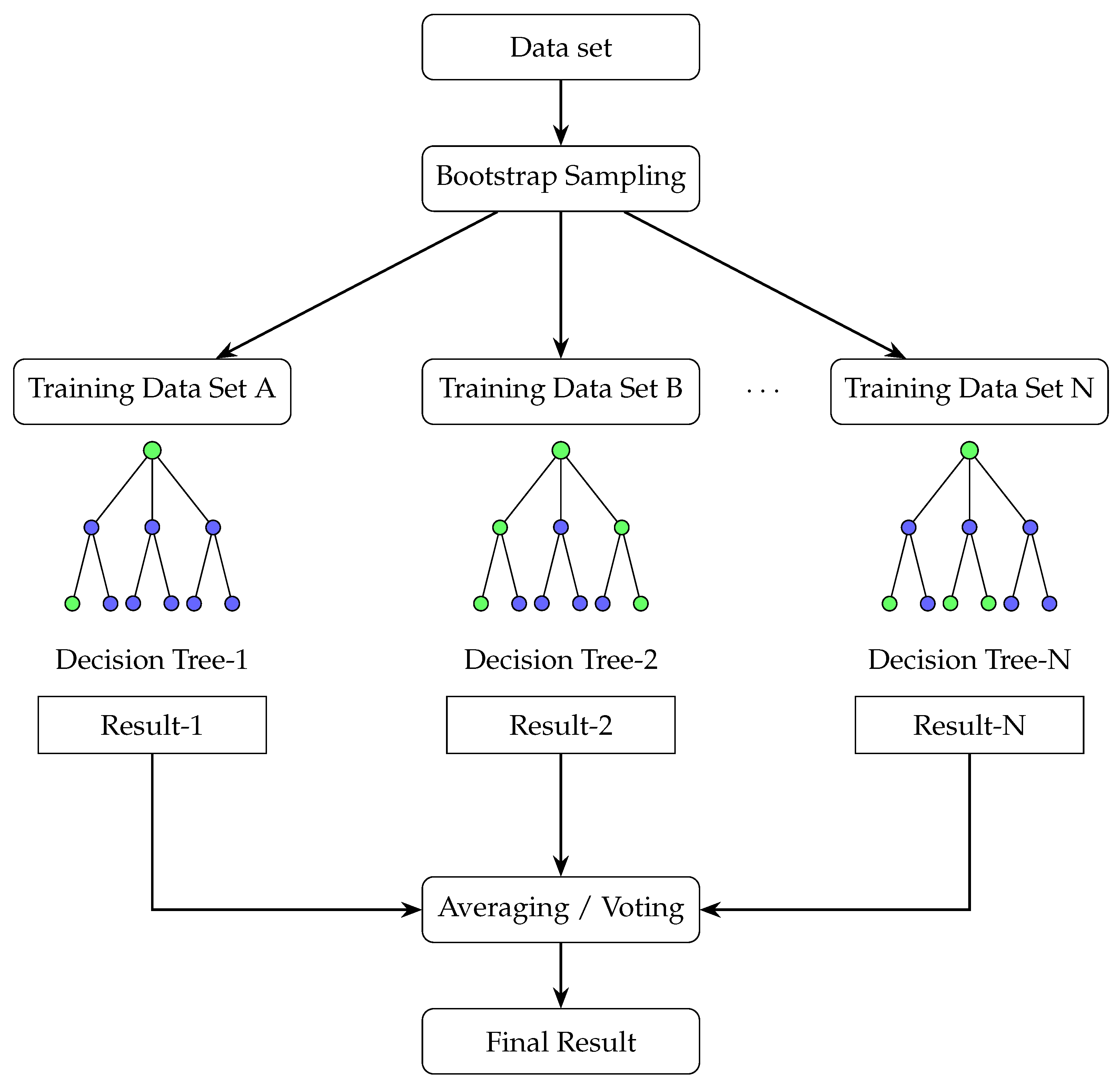
Decision trees are extensively utilized as foundational algorithms for both regression and classification tasks. Nonetheless, they are susceptible to overfitting, particularly when applied to complex problems characterized by high-dimensional input spaces. To mitigate the instability and overfitting tendencies inherent in single decision trees, the ensemble learning technique known as RF was proposed in 2001 [23]. RF integrates the principles of bootstrap aggregating (bagging) [24] and the stochastic subspace method [25], thereby enhancing model robustness and predictive accuracy. RF is an ensemble learning methodology that combines the predictions of multiple decision trees to derive a final output. During the training process, each base learner is trained on a bootstrap sample, generated through random sampling with replacement from the original dataset. Consequently, the samples not included in a given bootstrap subset are designated as out-of-bag samples, which serve as a means of internal validation and performance estimation. The inherent randomness of the method manifests in two aspects: first, the training samples for each decision tree are selected through random sampling with replacement; second, the feature subsets used for splitting at each node are also randomly sampled. This dual randomness serves to mitigate overfitting and enhances the diversity among individual decision trees. Consequently, the ensemble—composed of these diverse trees—is formed by averaging/voting their predictions [26]. This aggregation process results in a final model with improved accuracy and robustness. Figure 2 illustrates the architecture of the RF algorithm. The RF algorithm employs the Bootstrap resampling technique to randomly draw samples from the training dataset N times, with replacement. For each sampled dataset, k random features are independently selected, and N weak learners are constructed based on the Decision Tree algorithm. In regression tasks, the N weak learners are typically integrated to a strong learner by averaging their outputs, and the final prediction ${\widehat{f}}_{\mathrm{rf}}\left(\mathbf{x}\right)$ is obtained as:

$${\widehat{f}}_{\mathrm{rf}}\left(\mathbf{x}\right)={\displaystyle \frac{1}{N}}\sum _{i=1}^N{f}_i\left(\mathbf{x}\right),$$

(1)

where $f_i\left(\mathbf{x}\right)$ denotes the prediction of the i-th weak learner. In classification problems, however, the outputs of the weak learners are aggregated through a majority voting scheme, expressed as:

$$\begin{array}{c}\hfill {\overline{f}}_{\mathrm{rf}}\left(\mathbf{x}\right)=\mathrm{mode}{\left\{f_i\left(\mathbf{x}\right)\right\}}_{i=1}^N\end{array}$$

(2)

Figure 2. Flowchart of the RF algorithm. Adapted from [27].

In this study, RF was selected for both classification and regression tasks due to several advantages that make it suitable for geoscientific applications. RF handles non-linear and high-dimensional relationships effectively, is robust to outliers and noise, and reduces overfitting through bootstrap aggregation and random feature selection. These properties make it an appropriate choice for geological datasets, which often exhibit heterogeneity, skewed class distributions, and complex spatial variability [11,26].

3.2. Particle Swarm Optimization

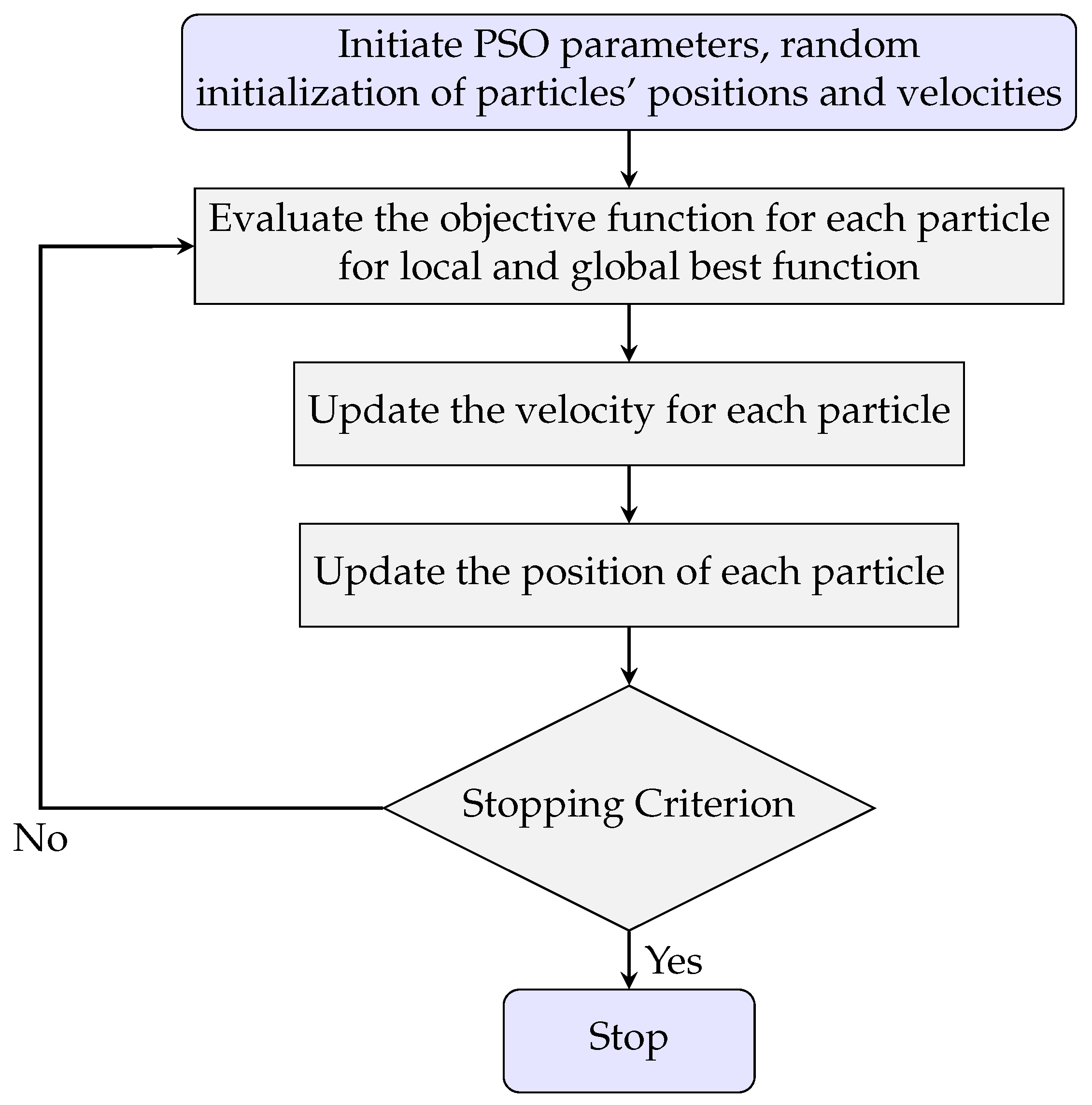
Particle Swarm Optimization (PSO) is a stochastic global optimization algorithm inspired by the social behavior of bird flocks and insect swarms [28]. It explores complex search spaces by simulating interactions among a population (swarm) of candidate solutions, referred to as particles. The algorithm begins by randomly initializing a swarm of particles that satisfy predefined criteria. These particles then iteratively update their positions in the search space by considering both their individual historical best positions and the best position found by the swarm as a whole until a stopping criterion is met [29,30]. In this study, PSO was chosen as a hyperparameter optimization strategy because it is computationally efficient, easy to implement, and requires fewer parameters compared to other strategies and algorithms [30]. A flowchart illustrating the PSO procedure is presented in Figure 3, and for further details, the reader is referred to [31,32].

Figure 3. Flowchart of the Particle Swarm Optimization (PSO) algorithm.

3.3. PSO-RF Algorithm

The performance of RF strongly depends on the choice of hyperparameters, particularly the number of trees (N) and the number of features randomly selected at each split (k). Selecting these parameters manually can be inefficient and may lead to suboptimal models. To address this, we coupled RF with PSO, which performs a guided search of the hyperparameter space to identify near-optimal values.

In this integrated PSO-RF approach, PSO iteratively explores candidate solutions for $(N,k)$, evaluates their performance using cross-validation, and updates the particle swarm until convergence. The best-performing configuration is then used to construct the final RF model, consisting of N decision trees. This optimized RF serves as the core predictive model in our workflow, applied both to the classification of geological domains (Stages 1–2) and to grade regression (Stage 3).

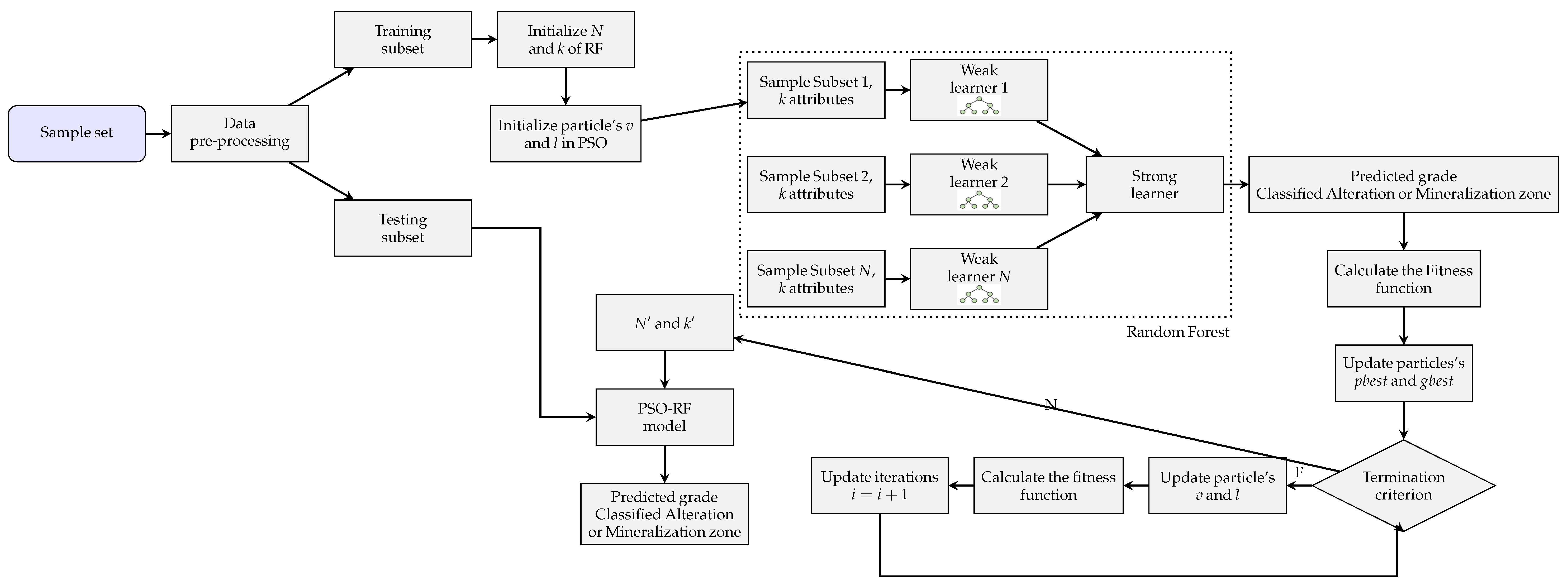
Following data pre-processing, the data set is partitioned into training and testing subsets. Within the PSO-RF framework, initial values are assigned to the RF parameters N and k, as well as to the particles’ positions (l) and velocities (v), which serve as the starting point for the optimization process. Each particle represents a potential solution to the optimization problem, which is finding the best values for hyperparameters. Each particle has a position $l_i$ = $(N_1,K_i)$ and a velocity $v_i$. At each iteration, each particle compares the cost value of its current position with its personal best (pbest) from previous iterations. If the current position achieves a lower cost, the particle updates its pbest. The global best position (gbest) is also updated whenever the best position found by the swarm in the current iteration outperforms any previously recorded global best. In this study, balanced Accuracy, Macro/Weighted F1-score, and Cohen’s $\kappa$ were employed as cost functions for geological domain classification, while the coefficient of determination (R²) and mean squared error (MSE) were used to assess grade estimation performance. After each iteration, the particles’ velocities and positions are updated according to the following equations:

$$v_i^{n+1}=w{v}_i^n+c_1{r}_1(p_{best,i}^n-l_i^n)+c_2{r}_2(g_{best,i}^n-l_i^n)$$

(3)

$$l_i^{n+1}=l_i^n+v_i^{n+1}$$

(4)

where $v_i^{n+1}$ and $v_i^n$ represent the velocity of particle i at iterations $n+1$ and n, respectively, and $l_i^{n+1}$ and $l_i^n$ denote the corresponding positions. The parameter w is the inertia weight, $c_1$ is the cognitive acceleration coefficient, and $c_2$ is the social acceleration coefficient [29,31]. $p_{best,i}^n$ indicates the best-known position of particle i, while $g_{best,i}^n$ denotes the best-known position across the entire swarm at iteration n. The terms $r_1$ and $r_2$ are random values drawn from a uniform distribution in the range $[0,1]$.

This iterative process continues for several iterations as defined by the user. Throughout it, PSO dynamically adjusts each particle’s position based on both its individual performance and the collective performance of the swarm. Ultimately, the final gbest obtained in the last iteration is selected as the optimal combination of hyperparameters ($N^{\prime }$ and $k^{\prime }$), which are subsequently used to construct the final RF model. By iteratively minimizing the cost function, PSO effectively identifies near-optimal parameter values.

It is important to note that the swarm size, inertia weight (w), and the acceleration coefficients ($c_1$ and $c_2$) are key elements of the PSO algorithm. These parameters control the search dynamics. The inertia weight w regulates the influence of a particle’s previous velocity, balancing exploration and exploitation of the search space. A high w promotes broader exploration, while a low w encourages finer, local search [33,34]. The coefficient determines how strongly a particle moves toward its own personal best (favoring individual learning), and it controls the influence of the swarm’s global best (encouraging collective learning) [35]. Proper adjustment of these parameters is essential to achieve a good balance between exploration and convergence. Finally, this optimized PSO-RF model is trained on the training subset to learn patterns in geological domains and grade distributions, and its predictive performance is evaluated using the testing subset. The complete algorithmic workflow is illustrated in Figure 4.

Figure 4. Compact flowchart of the PSO-RF algorithm for grade estimation or domain classification.

In this study, the search space for the optimization process was defined by setting the lower and upper bounds for each parameter as follows: number of trees ($n\_estimators$) = 10–200, maximum tree depth ($max\_depth$) = 5–30, and minimum number of samples required to split an internal node ($min\_samples\_split$) = 2–10. These parameter ranges were selected to provide sufficient flexibility for the PSO search while preventing overfitting and avoiding excessive computational cost. The PSO configuration included a swarm size of 50 particles and a maximum of 1000 iterations. The inertia weight (w) and the cognitive and social acceleration coefficients ($c_1$ and $c_2$) were set to 0.7298, 1.8, and 1.8, respectively, as recommended in previous studies [36]. These parameter settings ensure a good balance between exploration and exploitation during the optimization process.

It is worth mentioning that, to prevent spatial overfitting during hyperparameter optimization, we used a nested spatial cross-validation strategy. Because nearby samples tend to be similar, the data were divided at the drill hole level so that all samples from the same drill hole were kept together in either the training or testing set. This ensures spatial independence between the two subsets and avoids spatial leakage, which can otherwise produce overly optimistic accuracy. In the outer validation loop, 80% of the drill holes were used for training and the remaining 20% were reserved for testing. This division was repeated several times, and the final split was chosen to maintain a similar grade distribution and similar proportions of alteration and mineralization classes in both subsets. Within the training set, an inner cross-validation loop was used during PSO-based hyperparameter tuning, ensuring reliable model selection while minimizing overfitting.

4. Dataset and Geological Context

This study utilizes a dataset derived from exploratory drill holes at the Iju porphyry Cu deposit in Iran, which provides detailed information on copper grade, mineralization zones, and alteration zones. All assay intervals were composited to a uniform 2 m length to standardize sample support and minimize variability caused by differing sample lengths (Figure 5).

Figure 5. Location of drill holes data with information on (A) copper grades, (B) mineralization zones, and (C) alteration zones.

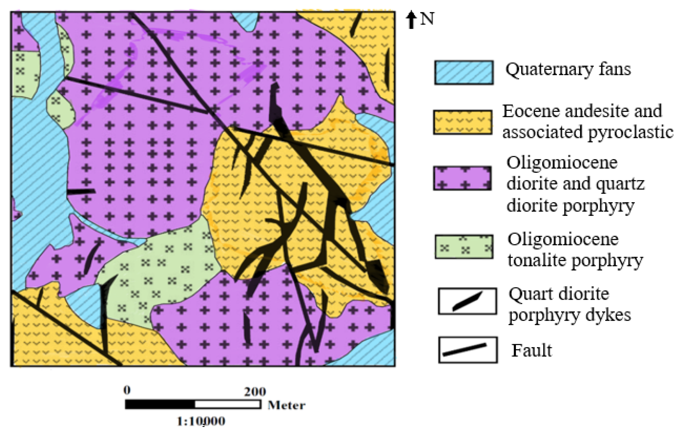
The Iju area is located 42 km north-west of Shahre-Babak county, Kerman province, and 140 km north-west of the Sarcheshme copper mine. The Iju deposit is situated on the southeast part of the Urmia-Dokhtar magmatic belt, which is characterized by numerous copper deposits such as the Chah-Firouze, Sarcheshme, Meiduk, and Chah-Messi [37,38,39]. The deposit is in a mountainous area with Eocene–Paleocene pyroclastic volcanic rocks that are intruded by Miocene quartz-diorite and tonalite rocks. Based on field investigations and core sample analyses, quartz diorite and tonalite are, respectively, penetrated to the host rocks [39,40,41] (Figure 6). In the Iju deposit, copper mineralization occurred in the form of disseminated stockworks. Chalcopyrite is the main copper mineral usually seen along with pyrite. Magnetite is observed as veins and veinlets in the central part of the study area. Little amounts of gypsums, anhydrite and molybdenite are detected in the study area. Based on the potassic, propylitic, extensive phyllic alterations, and mineralization style, the Iju is classified as a porphyry copper deposit. The Iju porphyry copper deposit comprises two distinct mineralization stages: hypogene (HYP) and supergene (SUP). Hypogene mineralization occurs as quartz–chalcopyrite ± pyrite ± magnetite stockwork veinlets and disseminated chalcopyrite [41]. Subsequent uplift and erosion exposed the hypogene ore to weathering, promoting sulfide oxidation, copper leaching, and supergene enrichment. This process generated three additional zones—leached (LEA), oxide (OXI), and supergene—alongside the primary hypogene zone. Deep groundwater levels have facilitated prolonged oxidation, with the leached zone dominated by iron oxides/hydroxides (hematite, goethite), silica, and locally jarosite. The oxide zone, developed beneath or adjacent to the leached zone, contains silicate, carbonate, and copper oxide minerals, but remains spatially limited and commonly intergrown with leached and supergene zones. Alteration zoning is a diagnostic feature of porphyry copper systems [42]. Field mapping and petrographic analyses at Iju delineate five principal alteration zones: potassic, propylitic, potassic–phyllic, phyllic, and argillic. The potassic zone (POT) is spatially restricted and frequently occurs in association with phyllic alteration (PHY), comprising secondary biotite, chlorite, and feldspar. This zone hosts the highest copper grades in the deposit [37,39]. Propylitic alteration (PRP) predominates in the western and southwestern sectors, particularly within volcanic unitsw and is characterized by epidote, chlorite, calcite, and sericite, reflecting a low-temperature hydrothermal overprint typical of distal zones in porphyry systems. Overprinting of potassic alteration by phyllic assemblages has produced a transitional potassic–phyllic zone containing quartz, sericite, and pyrite. The phyllic alteration is more extensive than the potassic zone, affecting much of the intrusive stock, especially the quartz diorite. Also, clay minerals, sericite, and chlorite indicate argillic alteration with limited spatial extent [39]. The composited drill-hole dataset used for modeling included only three alteration zones—potassic, propylitic, and phyllic—as the potassic–phyllic and argillic zones were too limited and sparsely sampled to be statistically represented. Accordingly, only these three alteration types were considered in the statistical analysis and grade estimation.

Figure 6. Geological map of the Iju deposit. Adapted from [37].

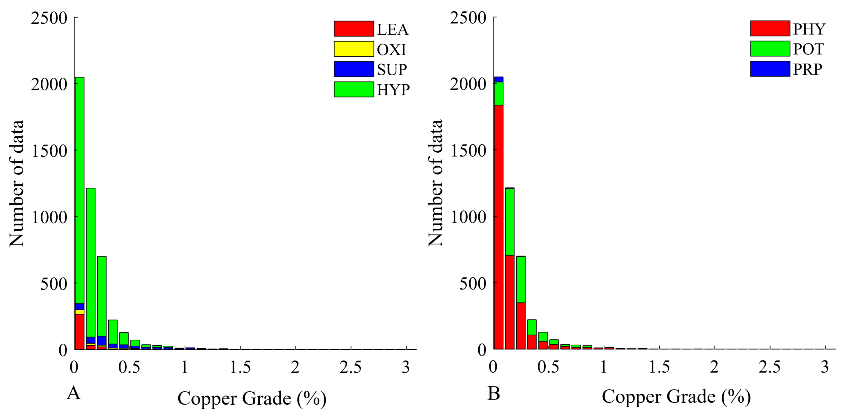
Table 1 presents the basic statistics of copper grade within the different mineralization and alteration zones. These tables indicate that the distribution of copper grade varies across both types of zones. This variability is further illustrated in the box plots and histograms shown in Figure 7 and Figure 8, which depict the copper grade distributions for the different mineralization and alteration zones.

Table 1. Basic statistics of copper grade (%) in different mineralization and alteration zones.

	Mineralization					Alteration
	Global	LEA	OXI	SUP	HYP	PHY	POT	PRP
Number of data	4526	320	90	322	3794	3173	1303	50
Mean value	0.164	0.058	0.259	0.445	0.147	0.134	0.239	0.072
Variance	0.036	0.009	0.074	0.169	0.018	0.033	0.036	0.004
Minimum	0.00	0.000	0.000	0.006	0.000	0.000	0.020	0.010
Lower quartile	0.050	0.010	0.060	0.170	0.050	0.040	0.130	0.030
Median	0.110	0.023	0.180	0.300	0.110	0.080	0.190	0.050
Upper quartile	0.210	0.070	0.380	0.620	0.200	0.160	0.290	0.090
Maximum	3.430	1.210	1.540	3.430	1.390	3.430	1.880	0.260

Figure 7. Box plots of Cu grade across various (A) mineralization and (B) alteration zones.

Figure 8. Histograms of Cu grade in different (A) mineralization and (B) alteration zones.

The variability of copper grade across different alteration and mineralization zones is a critical factor in the grade estimation process. For example, certain zones may exhibit higher mineralization due to favorable geochemical conditions, whereas others may show lower concentrations as a result of leaching or other post-depositional processes. While the box plots and histograms provide a clear visual indication of this variability, statistical tests were conducted to confirm its significance. Initially, several tests were considered, including the Levene’s test, the Fligner–Killeen test, Bartlett’s test, the Brown–Forsythe test, and ANOVA. However, preliminary Shapiro–Wilk testing indicated that the Cu grade data deviate from normality (Figure 8). Consequently, only Levene’s and the Fligner–Killeen tests were applied, as both are robust to non-normal data and provide reliable assessments of variance equality under non-Gaussian conditions. In Table 2, the p-values for both tests are presented. As shown, the variability of grade within both the alteration and mineralization zones differs significantly (p-value < 0.05). These differences must therefore be considered in the domaining process and subsequent grade estimation.

Table 2. p-value and statistics parameters for Levene’s and the Fligner–Killeen tests.

	Mineralization Zones		Alteration Zones
	p-Value	Statistics	p-Value	Statistics
Fligner–Killeen test	$7\times {10}^{-125}$	220.09	$8\times {10}^{-20}$	88.05
Levene test	$3\times {10}^{-133}$	577.69	$2\times {10}^{-5}$	10.82

5. Results and Discussion

5.1. Validating the PSO-RF Approach

As previously outlined, the proposed algorithm was implemented in three main stages. In the first stage, alteration zones were classified using the RF model. In the second stage, the RF model was applied to classify mineralization zones within the study area. Finally, the spatial coordinates of the sample data, along with the classified alteration and mineralization zones, were used as input variables to train the model and estimate the mineral grade in the study area. In all three stages, the PSO algorithm was employed to tune the hyperparameters of the RF model. To evaluate the effectiveness of the proposed PSO-RF approach, its performance was compared against that of the Support Vector Machine (SVM) models [43,44]. Similar to the proposed workflow, the SVM method also involved classifying the mineralization and alteration zones in the study area, which were subsequently used as input variables for training the model to estimate copper grade.

The comparative results presented in Table 3 highlight clear differences in the regression performance of the PSO-RF and SVM models. Overall, both models achieved satisfactory predictive ability, but their generalization performance on the testing dataset varied substantially. The PSO-RF model attained an R² value of 0.91 on the training set and 0.74 on the test set, with corresponding MSE values of 0.0034 and 0.0071. These results indicate that the proposed method not only captured the underlying relationships effectively during training but also maintained a relatively strong level of predictive accuracy when applied to unseen data. Although the test performance showed a slight decrease compared with the training set—as expected in most ML tasks—the reduction was moderate, reflecting good model generalization. In contrast, the SVM model achieved a slightly higher R² value (0.93) and lower MSE (0.0021) on the training data, suggesting that it fit the training set very well. However, its performance deteriorated notably on the test data, with the R² dropping to 0.61 and MSE increasing to 0.0083. This sharp contrast between training and testing performance points to potential overfitting, where the SVM model captured noise or specific patterns in the training data that did not generalize to new samples. It is worth mentioning that the hyperparameters of the SVM were optimized using a conventional grid search approach, while the PSO algorithm was employed exclusively for optimizing the hyperparameters of the RF models.

Table 3. Regression performance comparison between PSO-RF and SVM models.

PSO-RF				SVM
Train		Test		Train		Test
MSE	R2	MSE	R2	MSE	R2	MSE	R2
0.0034	0.91	0.0071	0.74	0.0021	0.93	0.0083	0.61

In a nutshell, the results demonstrate the robustness of the PSO-RF approach compared with SVM. The integration of Particle Swarm Optimization for tuning RF hyperparameters appears to have enhanced the balance between model complexity and generalization capability.

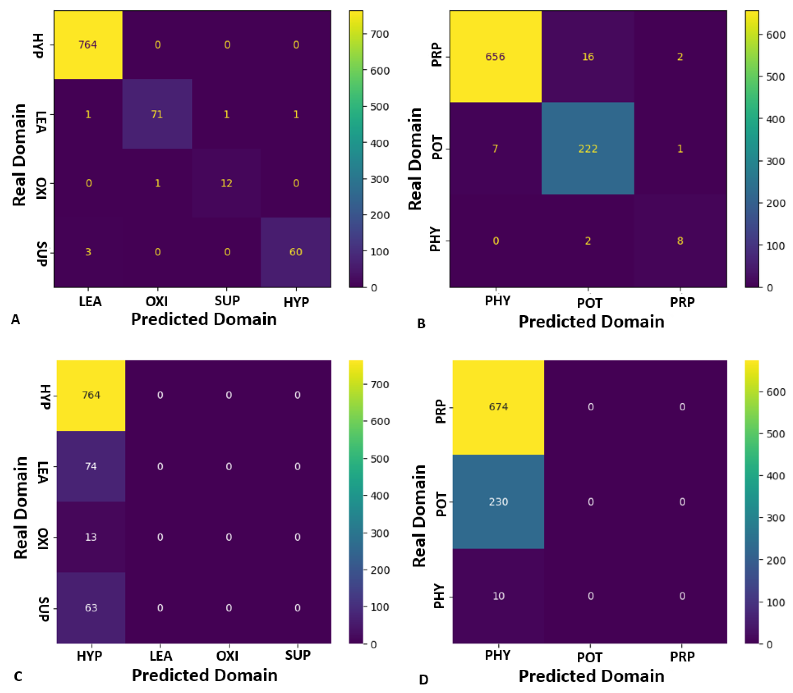
Figure 9 presents the confusion matrices corresponding to the classification of alteration (A, C) and mineralization (B, D) domains using the PSO-RF and SVM approaches. Panels A and B illustrate the results obtained with the PSO-RF model, whereas panels C and D show the performance of the SVM model.

Figure 9. Confusion matrices illustrating the classification performance of two models for geological domain prediction. (A) and (B) show the results obtained using the PSO-RF model for the classification of alteration zones and mineralization zones, respectively. (C,D) present the results for the SVM (Support Vector Machines) model applied to the same tasks.

As shown in Figure 9A,B, the PSO-RF model achieves high classification accuracy across all domain classes, with particularly strong performance in correctly identifying major classes such as Hypogene (HYP), Potassic (POT), and Propylitic (PRP). Importantly, it also maintains reasonable accuracy for minority classes, demonstrating robustness against class imbalance. In contrast, the SVM model (Figure 9C,D) exhibits a clear bias toward the majority classes, misclassifying nearly all minority-class instances into the dominant categories. This behavior substantially reduces the model’s reliability and underscores its limitations in handling imbalanced datasets. Overall, these findings confirm the effectiveness of the PSO-RF model for categorical domain classification in complex geological settings.

Beyond visual inspection of the confusion matrices, we computed robust classification metrics to quantify performance (Table 4). For alteration domains, the PSO-RF model achieved very high balanced accuracy (0.98), macro-F1 (0.98), and Cohen’s $\kappa$ (0.98), indicating excellent agreement across both majority and minority classes. In contrast, the SVM model reached moderate overall accuracy (0.84) but collapsed to the majority class, with a balanced accuracy of only 0.25, macro-F1 of 0.23, and $\kappa$ of 0.00. A similar pattern was observed for mineralization domains, where PSO-RF maintained substantial agreement ($\kappa =0.90$) and balanced accuracy of 0.70, whereas SVM again showed poor performance on minority classes (balanced accuracy = 0.33, $\kappa =0.00$). These results confirm that PSO-RF not only improves average classification accuracy but also provides fairer and more reliable predictions across all geological domains.

Table 4. Robust classification metrics for alteration and mineralization domains. OA = Overall Accuracy; BA = Balanced Accuracy; Macro/Weighted F1 = F1-score averaged across classes; $\kappa$ = Cohen’s Kappa.

Model/Task	OA	BA	Macro F1	Weighted F1	$\mathit{\kappa }$
RF—Alteration (A)	0.99	0.98	0.98	0.99	0.98
RF—Mineralization (B)	0.96	0.70	0.70	0.96	0.90
SVM—Alteration (C)	0.84	0.25	0.23	0.76	0.00
SVM—Mineralization (D)	0.74	0.33	0.28	0.63	0.00

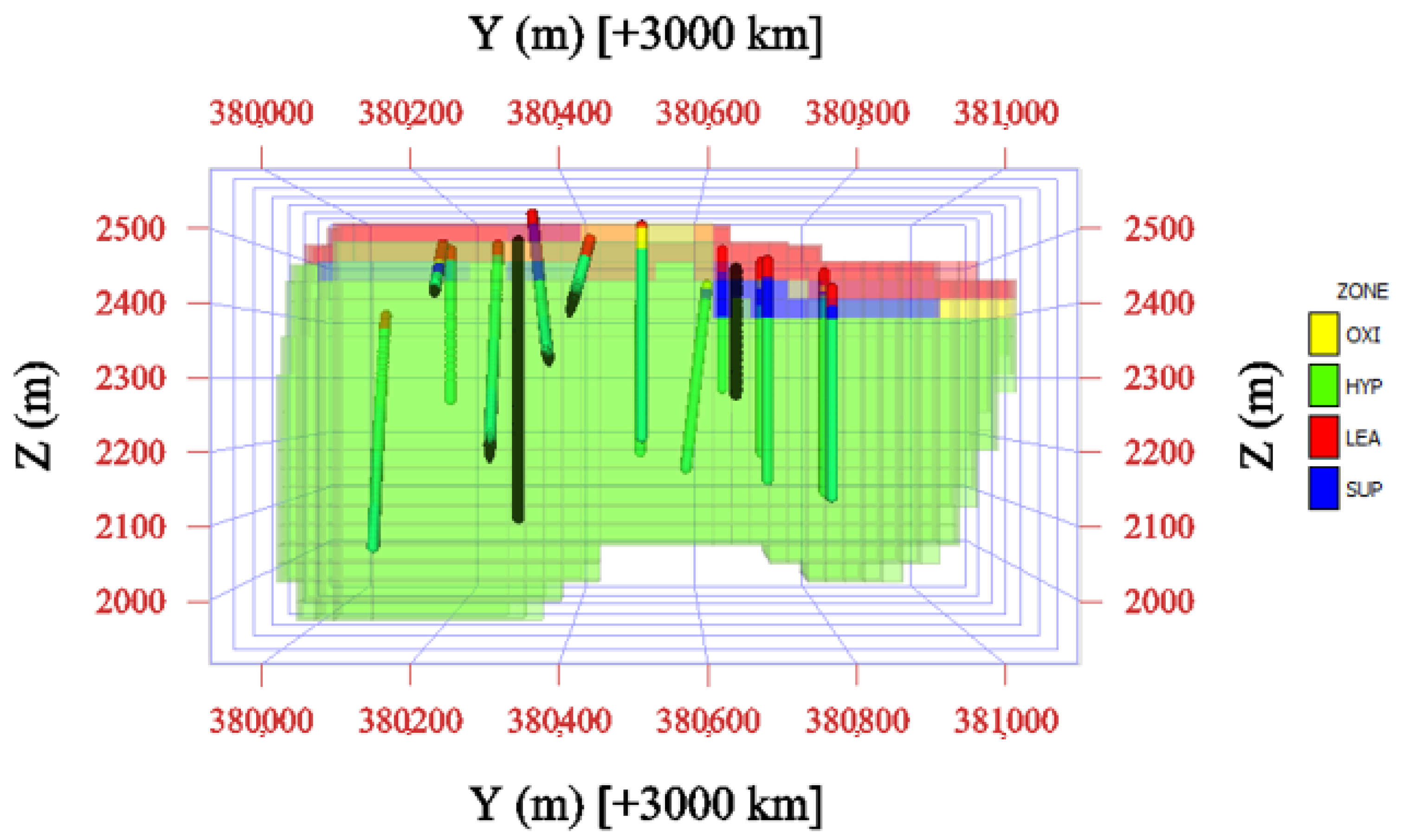
The spatial predictions of alteration and mineralization domains obtained from the PSO-RF classifiers are shown in Figure 10 and Figure 11, respectively. The predicted alteration map delineates the phyllic, potassic, and propylitic zones with clear spatial separation and lateral continuity, reproducing the zonation pattern observed in drillhole data. Similarly, the mineralization map reveals a coherent vertical progression from oxidized to hypogene zones, reflecting the expected supergene enrichment profile of the Iju deposit. These results confirm that the PSO-RF classifiers effectively capture both lithochemical and structural controls on alteration and mineralization patterns, supporting their use as input features for subsequent grade modeling.

Figure 10. Predicted alteration zones obtained using the PSO-RF model.

Figure 11. Predicted mineralization zones derived from the PSO-RF model.

5.2. Incorporating Geological Inputs into Ore Grade Predictions

To further investigate the impact of incorporating geological domain information into the grade estimation process, a sensitivity analysis was conducted under four different scenarios:

• Case A: Spatial coordinates only. In this scenario, the spatial coordinates of the sample data were used as the sole input features for training the PSO-RF model and for estimating copper grade.
• Case B: Spatial coordinates and alteration zones. In this case, the PSO-RF model was first applied to classify the alteration zones in the study area. The resulting classified alteration zones, together with the spatial coordinates, were then used as input features for training the PSO-RF model and estimating copper grade.
• Case C: Spatial coordinates and mineralization zones. Similar to Case B, the mineralization zones were first classified, and the classified zones, along with the spatial coordinates, were used as input features for training the PSO-RF model and estimating copper grade.
• Case D: Spatial coordinates, alteration zones, and mineralization zones. In this scenario, both the classified alteration zones and mineralization zones obtained from the previous steps were combined with the spatial coordinates. These three types of information were then used jointly as input features for training the PSO-RF model and estimating copper grade.

The R² and MSE values obtained for each model during training and subsequently evaluated on the testing set are summarized in Table 5.

Table 5. Performance comparison of different cases.

Model	MSE	R2
Model A	0.0073	0.73
Model B	0.0073	0.72
Model C	0.0072	0.73
Model D	0.0065	0.78

The results of the sensitivity analysis for the four scenarios are presented in Table 5. Model A, which used only spatial coordinates as input features, achieved an R² of 0.73 and an MSE of 0.0073, establishing the baseline performance. When geological domain information was incorporated individually—either alteration zones in Model B or mineralization zones in Model C—the results were only marginally different from the baseline. Model B showed a marginal decrease in performance (R² = 0.72), while Model C yielded nearly identical accuracy (R² = 0.73). In contrast, the most substantial improvement was obtained in Model D, where both alteration and mineralization zones were combined with spatial coordinates. This model achieved the highest accuracy (R² = 0.78) and the lowest error (MSE = 0.0065), demonstrating the complementary effect of integrating multiple geological domains.

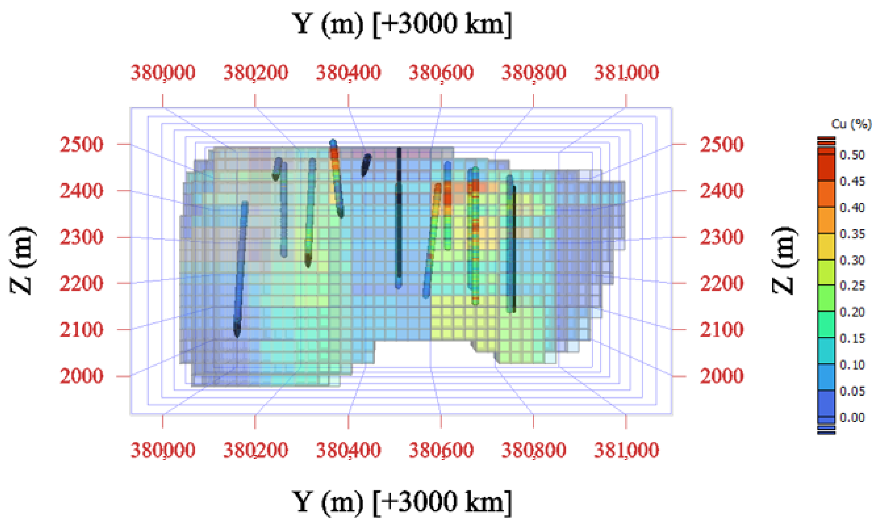
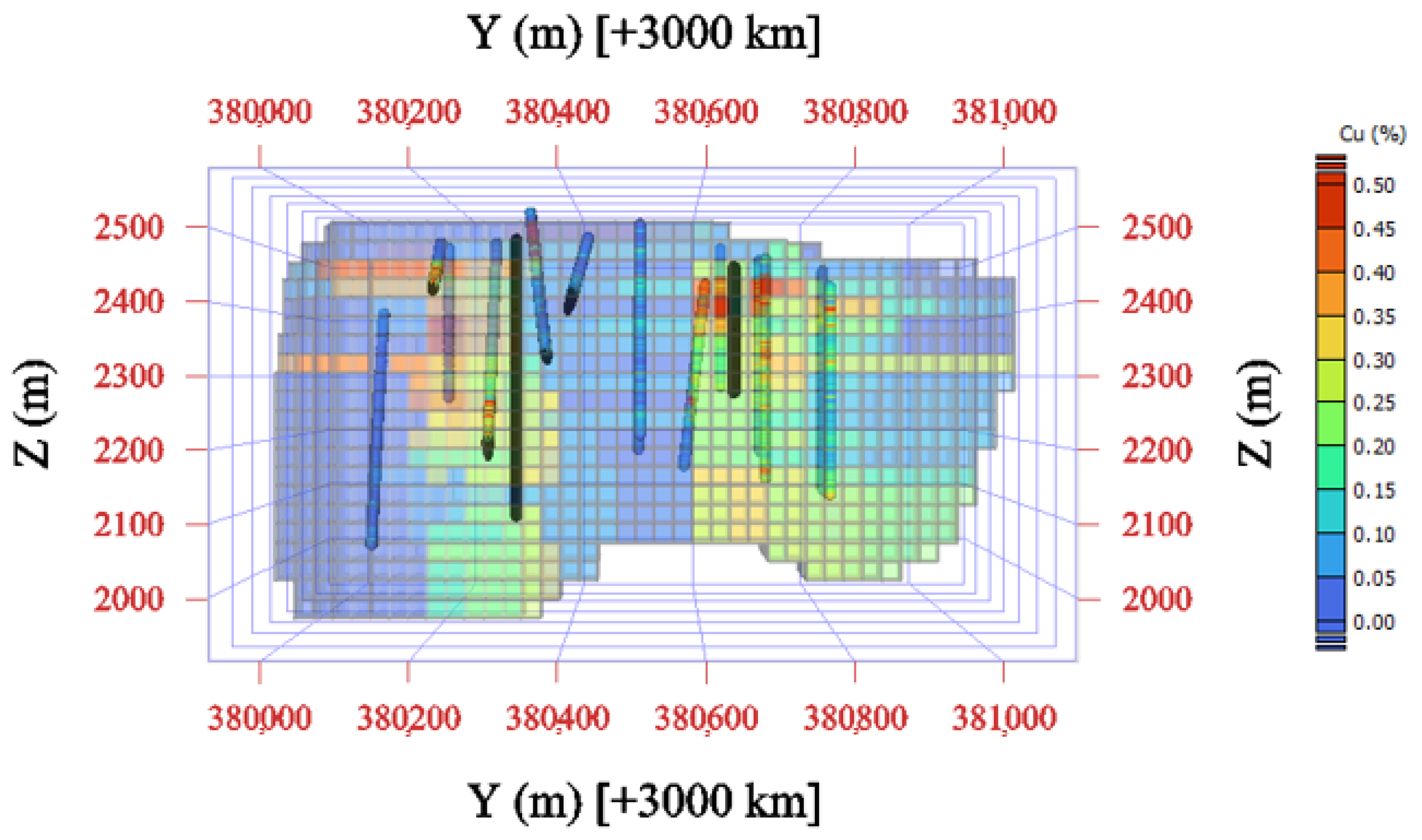
Figure 12 and Figure 13 illustrate the spatial distribution of predicted copper grades for two representative modeling scenarios. Figure 12 shows the results of Model A, which uses only spatial coordinates as predictive inputs. This configuration produces relatively smooth but geologically unrealistic grade patterns that fail to capture the spatial variability imposed by alteration and mineralization controls. In contrast, Figure 13 displays the results for Model D, which integrates both alteration and mineralization domains alongside spatial coordinates. The inclusion of these geological variables produces a distribution that better reflects the observed geological architecture, with grade variations aligning more closely to known alteration halos and mineralization zones. Models B and C, which individually incorporated alteration or mineralization information, are not shown because their grade distributions were visually and statistically similar to Model A. These results confirm that integrating multiple geological domains substantially improves the geological realism and interpretability of ML-based grade estimation models.

Figure 12. Predicted copper-grade distribution for Model A (coordinates only).

Figure 13. Predicted copper-grade distribution for Model D (coordinates + alteration + mineralization zones).

The findings indicate that spatial coordinates remain the dominant predictive factor for grade estimation in this case study. Although the incorporation of a single geological domain classification does not substantially improve performance, the combined inclusion of alteration and mineralization zones enhances model accuracy, underscoring the value of integrating multiple geological features in the estimation process. In fact, the superior performance of Model D (Table 5), which uses both alteration and mineralization domains, is due to the fact that each domain contributes different but complementary geological information. Alteration zoning reflects the intensity and distribution of hydrothermal fluid–rock interactions, which are strongly linked to the thermal and structural evolution of porphyry systems [42]. Mineralization zones, on the other hand, describe the transition between hypogene processes and supergene enrichment, which control the vertical redistribution of metals and the variability in copper grades [45]. When these two domains are integrated, they provide a more complete picture of the ore-forming processes. In practical terms, the model can better capture both the lateral alteration halos and the vertical geochemical zonation. This combination produces a synergistic effect, improving the structural and geochemical constraints in the model and leading to more accurate grade predictions than when using either domain alone.

Building on this, further improvements can be achieved within the proposed PSO-RF framework by incorporating structural properties alongside geological domain information as additional input variables, without necessitating new datasets. In this context, structural properties refer not to geological structures such as faults or fractures, but to geostatistical descriptors of local spatial variability—for example, grade gradients or local variograms derived from neighboring samples. This can be accomplished by explicitly capturing local variability through the grades of the nearest samples [46], thereby providing a more detailed representation of spatial heterogeneity.

While the proposed PSO-RF framework demonstrates robust performance, several limitations should be acknowledged. First, the reliability of grade predictions decreases in sparsely drilled or poorly sampled zones, where the model must extrapolate beyond the data-supported regions. Second, model performance is inherently dependent on the accuracy of the domain-classification stages, as misclassified alteration or mineralization zones may propagate uncertainty into the final grade estimates. Third, the current implementation assumes that the relationships derived from available samples remain valid across the entire block model, which may not always hold in geologically heterogeneous settings. These limitations could be mitigated in future studies by incorporating denser sampling, integrating structural and spatial-context features, or applying transfer-learning techniques to enhance model adaptability and generalization.

6. Conclusions

This study examined the impact of incorporating geological information—specifically mineralization and alteration zones—into a machine-learning workflow for copper grade estimation. A three-stage approach was developed in which RF classifiers, optimized using PSO, were first applied to classify mineralization and alteration zones. These classified domains, combined with spatial coordinates, were subsequently used as input features for grade prediction through an RF regression model.

To evaluate the contribution of geological information, copper grade was also predicted under alternative scenarios by varying the input data used to train the ML model: (i) spatial coordinates only, (ii) spatial coordinates with alteration zones, and (iii) spatial coordinates with mineralization zones. The results indicate that including either alteration or mineralization zones in isolation does not substantially improve predictive accuracy. However, the joint incorporation of both domains alongside spatial coordinates led to a meaningful improvement, demonstrating the complementary role of alteration and mineralization controls on grade distribution.

Furthermore, the predictive capability of the proposed PSO-RF framework was compared against SVM-based models. In this comparison, mineralization and alteration zones were classified with a support vector classifier and subsequently used with support vector regression for grade prediction. While both approaches yielded satisfactory results, the PSO-RF workflow consistently achieved higher predictive accuracy and demonstrated greater robustness to class imbalance. This underscores the advantage of optimizing RF hyperparameters through PSO in enhancing model generalization and improving grade estimation.

Overall, the findings highlight the value of integrating multiple geological domains into ML-based resource modeling. Although spatial coordinates remain the dominant predictor, the complementary inclusion of mineralization and alteration zones enhances model accuracy and geological consistency. The proposed framework provides a practical, computationally efficient, and geologically informed alternative for grade prediction in porphyry copper deposits.

References

1. Emery, X.; Séguret, S.A. Geostatistics for the Mining Industry: Applications to Porphyry Copper Deposits; CRC Press: Boca Raton, FL, USA, 2020. [Google Scholar]
2. Dumakor-Dupey, N.K.; Arya, S. Machine learning—A review of applications in mineral resource estimation. Energies 2021, 14, 4079. [Google Scholar] [CrossRef]
3. Lantuéjoul, C. Geostatistical Simulation: Models and Algorithms; Springer: Berlin, Germany, 2002. [Google Scholar]
4. Rossi, M.E.; Deutsch, C.V. Mineral Resource Estimation; Springer: Nw York, NY, USA, 2014. [Google Scholar]
5. Bassani, M.A.A.; Coimbra Leite Costa, J.F.; Deutsch, C.V. Multivariate geostatistical simulation with sum and fraction constraints. Appl. Earth Sci. 2018, 127, 83–93. [Google Scholar] [CrossRef]
6. Abulkhair, S.; Dowd, P.A.; Xu, C. Geostatistics in the presence of multivariate complexities: Comparison of multi-Gaussian transforms. Math. Geosci. 2023, 55, 713–734. [Google Scholar] [CrossRef]
7. Battalgazy, N.; Valenta, R.; Gow, P.; Spier, C.; Forbes, G. Addressing geological challenges in mineral resource estimation: A comparative study of deep learning and traditional techniques. Minerals 2023, 13, 982. [Google Scholar] [CrossRef]
8. Mahboob, M.; Celik, T.; Genc, B. Review of machine learning-based Mineral Resource estimation. J. South. Afr. Inst. Min. Metall. 2022, 122, 655–664. [Google Scholar] [CrossRef]
9. Plaza-Carvajal, J.; Maleki, M.; Khorram, F.; Emery, X. Assessing the Accuracy of Gaussian Transformations for Reproducing Statistical and Spatial Dependence Relationships in Multivariate Simulation: Plaza-Carvajal, Maleki, Khorram and Emery. Nat. Resour. Res. 2025, 24, 2993–3012. [Google Scholar] [CrossRef]
10. Tsae, N.B.; Adachi, T.; Kawamura, Y. Application of artificial neural network for the prediction of copper ore grade. Minerals 2023, 13, 658. [Google Scholar] [CrossRef]
11. Kaplan, U.E.; Topal, E. A new ore grade estimation using combine machine learning algorithms. Minerals 2020, 10, 847. [Google Scholar] [CrossRef]
12. Jain, G.; Pathak, P.; Bhatawdekar, R.M.; Kainthola, A.; Srivastav, A. Evaluation of machine learning models for ore grade estimation. In Proceedings of the International Conference on Geotechnical Challenges in Mining, Tunneling and Underground Infrastructures, Virtual, 20 December 2021; Springer: Singapore, 2021; pp. 613–624. [Google Scholar]
13. Mery, N.; Marcotte, D. Quantifying mineral resources and their uncertainty using two existing machine learning methods. Math. Geosci. 2022, 54, 363–387. [Google Scholar] [CrossRef]
14. Marquina Araujo, J.J.; Cotrina Teatino, M.A.; Mamani Quispe, J.N.; Noriega Vidal, E.M.; Vega Gonzalez, J.A.; Vega-Gonzalez, J.; Cruz-Galvez, J. Copper ore grade prediction using machine learning techniques in a copper deposit. J. Min. Environ. 2024, 15, 1011–1027. [Google Scholar]
15. Li, Z.; Zhan, Z.; Hu, J.; Yi, S.; Zhang, X.; Weng, Z.; Zhang, Z.; Ding, K. An Adaptive Generalized Regression Neural Network Approach for Ore Grade Estimation Considering Spatial Anisotropy. Nat. Resour. Res. 2025, 34, 2423–2442. [Google Scholar] [CrossRef]
16. Nasretdinova, M.; Madani, N.; Maleki, M. A stepwise cosimulation framework for modeling critical elements in copper porphyry deposits. Nat. Resour. Res. 2024, 33, 1439–1469. [Google Scholar] [CrossRef]
17. Erdogan Erten, G.; Yavuz, M.; Deutsch, C.V. Combination of machine learning and kriging for spatial estimation of geological attributes. Nat. Resour. Res. 2022, 31, 191–213. [Google Scholar] [CrossRef]
18. Dutta, P.J.; Emery, X. Classifying rock types by geostatistics and random forests in tandem. Mach. Learn. Sci. Technol. 2024, 5, 025013. [Google Scholar] [CrossRef]
19. Mery, N.; Marcotte, D. Assessment of recoverable resource uncertainty in Multivariate deposits through a simple machine learning technique trained using geostatistical simulations. Nat. Resour. Res. 2022, 31, 767–783. [Google Scholar] [CrossRef]
20. Maniteja, M.; Samanta, G.; Gebretsadik, A.; Tsae, N.B.; Rai, S.S.; Fissha, Y.; Okada, N.; Kawamura, Y. Advancing iron ore grade estimation: A comparative study of machine learning and ordinary kriging. Minerals 2025, 15, 131. [Google Scholar] [CrossRef]
21. Zaki, M.; Chen, S.; Zhang, J.; Feng, F.; Khoreshok, A.A.; Mahdy, M.A.; Salim, K.M. A novel approach for resource estimation of highly skewed gold using machine learning algorithms. Minerals 2022, 12, 900. [Google Scholar] [CrossRef]
22. Jafrasteh, B.; Fathianpour, N.; Suárez, A. Comparison of machine learning methods for copper ore grade estimation. Comput. Geosci. 2018, 22, 1371–1388. [Google Scholar] [CrossRef]
23. Breiman, L. Random forests. Mach. Learn. 2001, 45, 5–32. [Google Scholar] [CrossRef]
24. Breiman, L. Using iterated bagging to debias regressions. Mach. Learn. 2001, 45, 261–277. [Google Scholar] [CrossRef]
25. Ho, T.K. The random subspace method for constructing decision forests. IEEE Trans. Pattern Anal. Mach. Intell. 1998, 20, 832–844. [Google Scholar] [CrossRef]
26. Belgiu, M.; Drăguţ, L. Random forest in remote sensing: A review of applications and future directions. ISPRS J. Photogramm. Remote Sens. 2016, 114, 24–31. [Google Scholar] [CrossRef]
27. Wang, M.; Zhao, G.; Liang, W.; Wang, N. A comparative study on the development of hybrid SSA-RF and PSO-RF models for predicting the uniaxial compressive strength of rocks. Case Stud. Constr. Mater. 2023, 18, e02191. [Google Scholar] [CrossRef]
28. Eberhart, R.; Kennedy, J. A new optimizer using particle swarm theory. In Proceedings of the MHS’95 Proceedings Sixth International Symposium on Micro Machine and Human Science, Nagoya, Japan, 4–6 October 1995; Available online: http://www.ppgia.pucpr.br/alceu/mestrado/aula3/PSO_2.pdf (accessed on 10 October 2025).
29. Maleki, M.; Baeza, D.; Soltani-Mohammadi, S.; Madani, N.; Díaz, E.; Anguita, F. Optimising the placement of additional drill holes to enhanced mineral resource classification: A case study on a porphyry copper deposit. Int. J. Min. Reclam. Environ. 2025, 39, 134–151. [Google Scholar] [CrossRef]
30. Sahab, M.G.; Toropov, V.V.; Gandomi, A.H. A review on traditional and modern structural optimization: Problems and techniques. In Metaheuristic Applications in Structures and Infrastructures; Elsevier: Amsterdam, The Netherlands, 2013; pp. 25–47. [Google Scholar]
31. Kennedy, J.; Eberhart, R. Particle swarm optimization. In Proceedings of the ICNN’95—International Conference on Neural Networks, Perth, WA, Australia, 27 November–1 December 1995; IEEE: Piscataway, NJ, USA, 1995; Volume 4, pp. 1942–1948. [Google Scholar]
32. Freitas, D.; Lopes, L.G.; Morgado-Dias, F. Particle swarm optimisation: A historical review up to the current developments. Entropy 2020, 22, 362. [Google Scholar] [CrossRef]
33. Cheng, Y.M.; Li, L.; Chi, S.c.; Wei, W. Particle swarm optimization algorithm for the location of the critical non-circular failure surface in two-dimensional slope stability analysis. Comput. Geotech. 2007, 34, 92–103. [Google Scholar] [CrossRef]
34. Ferland, J.A.; Amaya, J.; Djuimo, M.S. Application of a particle swarm algorithm to the capacitated open pit mining problem. In Autonomous Robots and Agents; Springer: Berlin/Heidelberg, Germany, 2007; pp. 127–133. [Google Scholar]
35. Fernández-Martínez, J.; García-Gonzalo, E.; Fernández-Alvarez, J. Theoretical analysis of particle swarm trajectories through a mechanical analogy. Int. J. Comput. Intell. Res. 2008, 4, 93–105. [Google Scholar] [CrossRef]
36. Qi, C.; Fourie, A.; Chen, Q. Neural network and particle swarm optimization for predicting the unconfined compressive strength of cemented paste backfill. Constr. Build. Mater. 2018, 159, 473–478. [Google Scholar] [CrossRef]
37. Mirnejad, H.; Mathur, R.; Hassanzadeh, J.; Shafie, B.; Nourali, S. Linking Cu mineralization to host porphyry emplacement: Re-Os ages of molybdenites versus U-Pb ages of zircons and sulfur isotope compositions of pyrite and chalcopyrite from the Iju and Sarkuh porphyry deposits in Southeast Iran. Econ. Geol. 2013, 108, 861–870. [Google Scholar] [CrossRef]
38. Mirnejad, H.; Raeisi, D.; Heidari, F. Geochemistry and petrogenesis of tonalite from Iju area, northwest of Shahr-e Babak (Kerman province), with emphasis on adakitic magmatism. Petrol. J. 2015, 6, 197–210. [Google Scholar]
39. Zarasvandi, A.; Rezaei, M.; Pourkaseb, H.; Asadi, S.; Azimzadeh, A.M. Characterization of potassic alteration in the Iju porphyry copper deposit using mineral chemistry of biotite and chlorite. Petrol. J. 2018, 8, 67–86. [Google Scholar]
40. Aghazadeh, M.; Hou, Z.; Badrzadeh, Z.; Zhou, L. Temporal–spatial distribution and tectonic setting of porphyry copper deposits in Iran: Constraints from zircon U–Pb and molybdenite Re–Os geochronology. Ore Geol. Rev. 2015, 70, 385–406. [Google Scholar] [CrossRef]
41. Golestani, M.; Karimpour, M.H.; Shafaroudi, A.M.; Shahri, M.R.H. Geochemistry, U-Pb geochronology and Sr-Nd isotopes of the Neogene igneous rocks, at the Iju porphyry copper deposit, NW Shahr-e-Babak, Iran. Ore Geol. Rev. 2018, 93, 290–307. [Google Scholar] [CrossRef]
42. Guilbert, J.M.; Park, C.F., Jr. The Geology of Ore Deposits; Waveland Press: Long Grove, IL, USA, 2007. [Google Scholar]
43. Cortes, C.; Vapnik, V. Support-vector networks. Mach. Learn. 1995, 20, 273–297. [Google Scholar] [CrossRef]
44. Noble, W.S. What is a support vector machine? Nat. Biotechnol. 2006, 24, 1565–1567. [Google Scholar] [CrossRef] [PubMed]
45. Sillitoe, R.H. Porphyry copper systems. Econ. Geol. 2010, 105, 3–41. [Google Scholar] [CrossRef]
46. Soltani-Mohammadi, S.; Hoseinian, F.S.; Abbaszadeh, M.; Khodadadzadeh, M. Grade estimation using a hybrid method of back-propagation artificial neural network and particle swarm optimization with integrated samples coordinate and local variability. Comput. Geosci. 2022, 159, 104981. [Google Scholar] [CrossRef]
Disclaimer/Publisher’s Note: The statements, opinions and data contained in all publications are solely those of the individual author(s) and contributor(s) and not of MDPI and/or the editor(s). MDPI and/or the editor(s) disclaim responsibility for any injury to people or property resulting from any ideas, methods, instructions or products referred to in the content.
Article Metrics
Citations
Article Access Statistics
Article metric data becomes available approximately 24 hours after publication online.