Abstract
To understand and optimise downstream processing of ores, reliable information about mineral abundance, association, liberation and textural characteristics is needed. Such information can be obtained by using Optical Image Analysis (OIA) in reflected light, which can achieve good discrimination for the majority of minerals. However, reliable automated segmentation of non-opaque minerals, such as quartz, which have reflectivity close to that of the epoxy they are embedded in, has always been problematic. Application of standard thresholding techniques for that purpose typically results in significant misidentifications. This paper presents a sophisticated segmentation mechanism, based on enhanced thresholding of non-opaque minerals developed for Commonwealth Scientific and Industrial Research Organisation’s (CSIRO) Mineral5/Recognition5 OIA software, which significantly improves segmentation in many applications. The method utilises an enhanced image view using an adjusted reflectivity scale for more precise initial thresholding, and comprehensive clean-up procedures for further segmentation improvement. For more complex cases, the method also employs specific particle border thresholding with subsequent selective erosion-based “reduction to borders”, while “particle restoration” prevents the detachment of non-opaque grains from larger particles. This method can be combined with “relief-based discrimination of non-opaque minerals” to achieve improved overall segmentation of non-opaque minerals.
1. Introduction
Ore characterisation is an essential part of almost all stages in mineral industry production, from exploration [1,2] to the design of optimal beneficiation workflows [3,4,5] and product control [6]. Along with mineral abundance, which can be provided by quantitative X-ray diffraction (XRD) [7], information about the mineral association, liberation and textural peculiarities is required [8,9,10]. The latter can be obtained by using Scanning Electron Microscopy (SEM) [11,12,13,14,15] or Optical Image Analysis (OIA) [16,17,18,19,20,21].
The choice of a particular image-based characterisation technique may depend on ore mineralogy and texture. For fine porous textures, or for minerals with close chemical composition (such as various oxides and oxyhydroxides of the same element) and/or close backscattered signal (hematite, magnetite, hydrohematite in iron ore), OIA may be preferential. For example, a comparison of results from OIA and SEM characterisation of the same iron ore samples by Donskoi et al. [22] demonstrated significant misidentification of magnetite and hematite by SEM, and also misidentification of highly porous hematite as goethite. Being a scanning method, SEM also has restrictions in terms of combined resolution and speed. To increase measurement speed, SEM often relies on large steps (5 µm and higher) between measured points. Its resolution is also limited by excitation volume, which can exceed 1 µm, especially for porous media. This makes OIA the preferential method for the textural classification of ores and when working with large imaging areas. OIA also allows for the segmentation of different grains of the same mineral [23,24,25] or enables phases to be distinguished based on their bi-reflectance [26].
On the other hand, if phases present in the epoxy block have lower and similar reflectivity, such as the common gangue minerals for the goethitic iron ores: kaolinite, gibbsite and dolomite, SEM methods can be preferable to OIA. Other typical examples include the differentiation of non-opaque minerals and epoxy resin, or when the relationship between mineral reflectivity and mineral identification is uncertain, or when the measurement of chemical composition is of importance. For OIA, reliable segmentation of minerals with similar reflectivity, or with reflectivity close to that of epoxy, is a well-known problem [27,28]. However, recent developments such as the significant increase in sensitivity of digital cameras, the switch from greyscale to colour imaging and the increase in computing power allowing more complex image analysis processing, now enable better segmentation of different minerals and textures by OIA. For example, Lane et al. [29] demonstrated OIA segmentation of non-opaque minerals such as apatite, amphibole, calcite and garnet in reflected light.
Nevertheless, segmentation of some other non-opaque minerals, such as quartz, in reflected light OIA is problematic, due to the very similar reflectivity of such non-opaque minerals and epoxy resin used in polished block preparation. The reflectivity of epoxy can be slightly modified by adding different dyes, which helps to increase the difference in reflectivity between quartz and epoxy [28], but that may still not be enough for reliable quartz segmentation. On the topic of block preparation, it should also be mentioned that due to the noticeable difference in density between quartz (2.65 g/cm3) and minerals such as magnetite (~5.15 g/cm3), strong density segregation among particles may occur in epoxy blocks, affecting all obtained data [30]. For reliable characterisation of samples containing relatively light non-opaque minerals and much heavier ore minerals, vertical block sections should be used [30].
Until recently, only a few publications proposed possible solutions for the automated segmentation of quartz in reflected light optical microscopy (RLOM). The latest approaches to the problem involve deep learning techniques, which allow up to 90%–95% of non-opaque areas to be identified [31,32]. It should be noted that such techniques are quite time-consuming, and it was unclear how long image processing may take. Even though the deep learning technique approach can be considered fairly prospective, there are certain considerations to be taken into account. To properly characterise a sample, quite often a large sample area including hundreds of images at a proper resolution has to be processed, which can make the time constraints very important. In addition, such systems are usually “trained” on a certain set of samples, and it is unclear how they will perform for samples significantly different from the training sets (in terms of particle shape, magnification during imaging, etc.).
Delbem et al. [33,34] developed a digital image analysis system called Opt-Lib, which facilitated the differentiation, classification and quantification of iron oxide/hydroxide minerals and quartz. In order to segment quartz in the samples, the system enhanced the borders between quartz and epoxy resin resulting from optical relief. For that purpose, they used the ‘‘UnsharpMask’’ filter [35], and further applied a comprehensive algorithm distinguishing resin and quartz. Poliakov and Donskoi [36] also proposed a comprehensive quartz segmentation method based on the utilisation of quartz borders. This method, as well as the enhanced thresholding method presented in this paper, are both used to perform non-opaque mineral segmentation in the Mineral5/Recognition5 OIA software developed by the Commonwealth Scientific and Industrial Research Organisation (CSIRO), Australia [37].
The problems with the segmentation of non-opaque minerals in RLOM have been discussed by many authors [31,32,34,38]. Iglesias et al. [31] demonstrated that attempts to segment quartz from the epoxy resin might result in the partial selection of resin and other dark minerals. However, the approach used in the Mineral5/Recognition5 software enables the operator to significantly reduce the instances of such misidentifications and very often to fully avoid them.
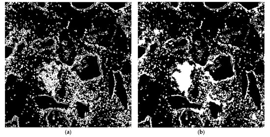
First of all, it has to be ensured that the reflectivity of the non-opaque minerals present in an ore, most often quartz, is different from that of epoxy resin. To achieve this, a suitable resin, different from what is typically used for mineralogy studies, could be utilised. Alternatively, and this approach is typically used by the authors, a significant amount of Epodye can be added to epoxy as suggested by Neumann and Stanley [28]; the authors use 0.625 g of Epodye per 25 g of resin, which is about 5 times more than the standard ratio. Figure 1 provides examples of images where the same iron ore sample was embedded into epoxy blocks with the addition of Epodye as suggested above and without Epodye. Quartz particles in Figure 1a (with Epodye) are fairly contrasted with epoxy, while the block without Epodye in Figure 1c had to be overpolished to make quartz visible by relief. Carefully selected optimal thresholding of quartz in both images also clearly demonstrates much better segmentation for the image with Epodye.
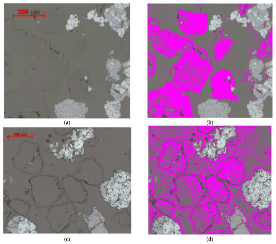
Figure 1.
Iron ore images from two epoxy blocks from the same sample, with (a) and without (c) Epodye, taken at magnification ×200, and optimal segmentation of quartz by thresholding, (b,d) correspondingly.
Secondly, all opaque minerals in the sample must be segmented before the segmentation of quartz or other non-opaque minerals. The multi-thresholding approach used in Mineral5 [21] enables this process to be performed with very high accuracy. Identification of opaque minerals before non-opaque minerals removes their corresponding areas from consideration during further non-opaque mineral segmentation.
Thirdly, segmentation of non-opaque minerals, apart from the enhanced thresholding step itself, includes a number of comprehensive steps allowing for the removal of areas incorrectly identified during thresholding. Finally, the enhanced thresholding of non-opaque minerals can be used together with relief-based segmentation, significantly increasing the reliability of non-opaque mineral identification.
The approach described in this article allows the authors to perform reliable quartz segmentation in almost all cases related to iron-ore characterisation. Depending on the specifics of the sample, it provides a good complementary or a fully alternative option to improve overall non-opaque mineral segmentation. However, some problems may occur when a sample has more than one non-opaque mineral. The Mineral5/Recognition5 system currently supports the specific non-opaque mineral identification discussed in this paper for one mineral per sample. However, segmentation of more than one non-opaque mineral per sample can still be performed, employing recent developments in the software, including flexible mineralogy [39,40], multi-thresholding [21] and textural identification techniques [41] where applicable to segment the additional non-opaque minerals.
2. Use of Enhanced Thresholding for Non-Opaque Segmentation
While border-based non-opaque mineral segmentation, described by Poliakov and Donskoi [36], provides good results for a significant proportion of samples, there are cases when border visibility is not good enough for reliable border-based identification. Our experience shows that images taken at higher magnification (which, as a general rule, corresponds to finer size fractions) tend to have lower border visibility. Therefore, the Enhanced Thresholding method proposed here is more useful for higher magnifications, while for lower magnifications the border-based method should be considered first.
It is also common for individual particle border visibility to vary significantly. Figure 2 provides an example of an optical image of iron ore fines in an epoxy block with Epodye displaying three non-opaque particles, two of which (A and B) are well visible with clear borders, while the third (C), presumably a different non-opaque mineral, is nearly invisible and has a different texture, with significant breaks in the border as well. While border-based identification can easily identify particles A and B, it may fail to identify C. It highlights that, in certain cases, border-based identification alone can underestimate the amount of non-opaque minerals in a sample.
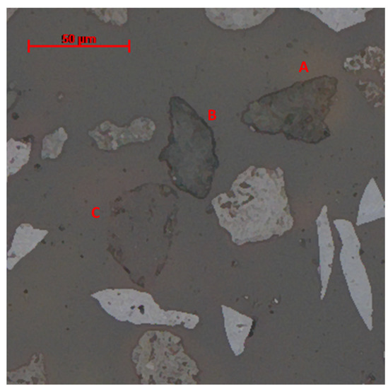
Figure 2.
Non-opaque particles at magnification ×200 with different border and body visibility: high (A, B) and low (C).
In order to improve the identification of particles with low border visibility, the Non-Opaque Identification Module of CSIRO’s Mineral5 OIA software was extended with an alternative set of algorithms that successfully perform threshold-based identification. As discussed in the introduction, it is typically impossible to perfectly identify non-opaque material by traditional thresholding due to its close reflectivity with epoxy resin, which results in a high amount of noise readings in the epoxy. Still, in many cases it can provide acceptable results, especially when used in conjunction with border-based techniques, which will be discussed further in the paper. Figure 3 outlines the operations related to threshold-based non-opaque identification and their location within Mineral5 workflow. The detailed description of those operations and examples of their application to particular tasks will be provided further. The flowchart does not focus on image analysis steps not directly related to non-opaque identification; readers can find a full Mineral5 flowchart in [37], while [21] provides detailed descriptions of corresponding operations.
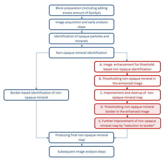
Figure 3.
Enhanced threshold-based identification of non-opaque minerals (red) within Mineral5 workflow. Optional “reduction to border” steps highlighted with pink.
In order to explain the non-opaque mineral segmentation methodology in detail and visualise the steps, the section of the Non-Opaque Identification module containing the controls responsible for threshold-based identification is shown in Figure 4. The section consists of several parts and, as the actual enhanced threshold-based identification (steps A–C in Figure 3) will be considered first, the controls related to it are active. Further enhancement to the algorithm, “reduction to borders” (steps D–E in Figure 3), will be discussed in the next section, so in Figure 4 the “Use borders” checkbox, activating the corresponding controls, is unchecked and the greyed-out controls to the right of the discussed section of the Non-Opaque Identification module can be temporarily ignored.
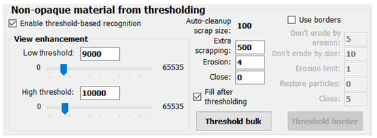
Figure 4.
Threshold-based identification frame with “Use borders” section disabled.
The controls on the form can be easily understood by an experienced operator of OIA software. The execution of threshold-based routines within the Non-Opaque Identification module is controlled by the “Enable threshold-based recognition” checkbox, which can switch the entire procedure on and off.
As it can be seen from Figure 2, some of the non-opaque minerals in the sample (represented by particle C) cannot be easily distinguished in the original image either by reflectivity or by border. Figure 4 shows two “View enhancement” controls allowing the operator to convert a certain narrow reflectivity range into a much wider range, which is therefore more clearly visible and easier to use for threshold adjustment. In each of the three colour channels, all image areas that have reflectivity less than “Low threshold” will be presented as black, while all areas with reflectivity higher than “High threshold” will be presented as completely white. The reflectivity range in between these thresholds will be stretched to the full visible range between black and white (0 to 65,535 pixel brightness in a 16-bit channel). If the chosen reflectivity range includes non-opaque material, the actual visibility of non-opaque particles to the operator improves significantly. Figure 5a provides an example of an early step of such enhancement, with the selected range still too wide. Figure 5b,c represent subsequent unsuccessful attempts to narrow this range down, where the actual selection is below and above the optimal range correspondingly, while Figure 6 shows the result of the most appropriate choice of thresholds allowing for a much better view of particle C from Figure 2. The analysis step outlined here is shown as step A in Figure 3 and is formally described as Algorithm S1 in Supplementary Material.
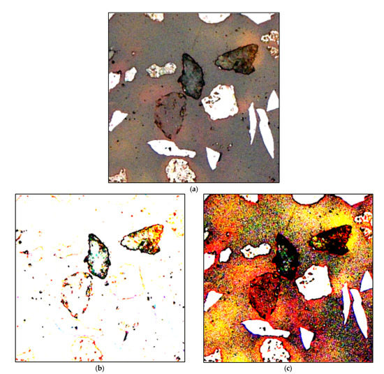
Figure 5.
Generating “enhanced” view of the image from Figure 2, early steps: (a) selected range too wide (low threshold = 7000, high threshold = 15,000); (b) selected range below the optimal range (low threshold = 8000, high threshold = 9000); and (c) selected range above the optimal range (low threshold = 10,000, high threshold = 11,000).
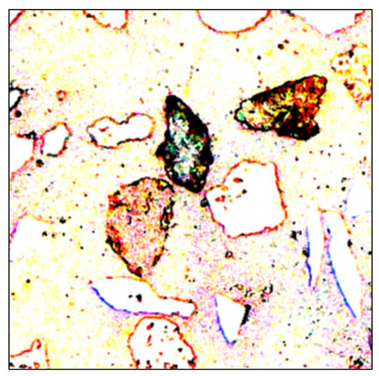
Figure 6.
“Enhanced” view of the image from Figure 2 with a suitable selected reflectivity range (low threshold = 9000, high threshold = 10,000).
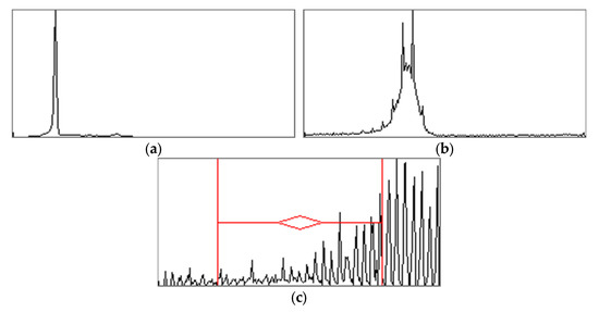
Figure 7 shows reflectivity histograms in blue channel for the original and enhanced images. The highest peak in Figure 7a (original image) corresponds to the reflectivity of epoxy and non-opaques and contains no discernible details. Figure 7b (partially enhanced image from Figure 5a) provides a somewhat more detailed view of that reflectivity range; however, it is the histogram in Figure 7c (enhanced image from Figure 6) that allows for selecting proper thresholds for non-opaque mineral identification. This histogram corresponds to the reflectivity range near the left-hand slope of the epoxy peak and is very discrete as the original reflectivity range has been highly stretched.
This discussion will focus on the segmentation of particle C, as particles A and B can be easily identified using a border-based method [36]. As a result of the applied transformation, the image is noticeably grainy, as a significant amount of information outside the selected reflectivity range has been destroyed. However, it serves the purpose of improving the visibility of the non-opaque particle, which can now be thresholded [42] by clicking the “Threshold bulk” button, as shown in Figure 4, which corresponds to workflow step B in Figure 3. It is important to emphasise that, as discussed by Poliakov and Donskoi [36] and Iglesias et al. [31], such a thresholding, even if the identification of non-opaque mineral area is partial and incomplete, will produce a significant amount of false readings within epoxy, as evident in Figure 8. It is also almost impossible to select the whole non-opaque particle without also selecting very significant areas of epoxy. As a result, the map obtained from thresholding requires significant cleanup and improvement, which is performed by subsequent procedures and controlled by the rest of the parameters on the form in Figure 4.
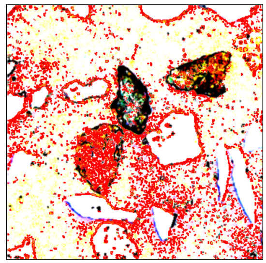
Figure 8.
Thresholding of non-opaque particle by “Threshold bulk” (red—thresholded phase, for original image see Figure 2).
The major procedures used for such a cleaning are the standard image analysis operations of scrapping and erosion. The “Auto-cleanup” value in Figure 4 shows the settings for particle scrap taken from the “Particle identification” routine [21], which segments the opaque areas of all particles. Objects/particles below this size are not considered important for sample characterisation and will be automatically scrapped here as well. An “Extra scrapping” value can be set in the appropriate textbox of Figure 4 if necessary and allows for scrapping of larger noise areas. This function is important for the discussed operation, because non-opaque thresholding, which selects the reflectivity range very close to that of epoxy, tends to produce more noise compared to opaque thresholding. The “Erosion” operation in Figure 4 sets the value for another cleanup mechanism, consisting of initial erosion of the map and subsequent dilation (this erosion/dilation cycle is also known as “Opening”), allowing restoration of the non-opaque particle area. Thin objects, such as the “shades” in epoxy associated with opaque particle boundaries clearly evident in Figure 6 and Figure 8, will be fully eliminated by erosion and therefore not restored.
Before the cleanup operations, as the identified non-opaque area is grainy and not fully continuous, its segmentation can be improved by providing a value for the “Close” operation (dilation/erosion cycle) and/or checking the “Fill after thresholding” checkbox in Figure 4. In the scenario described here, the original thresholded map from Figure 8 is shown in Figure 9a, and the result of the fill operation is shown in Figure 9b. The “Close” operation is not applied in this particular case, to avoid excessive noise clustering.
The fill operation “solidifies” the non-opaque particle in question but also has a similar effect on some noise readings. Therefore, a strong cleanup (i.e., scrap = 500 and erosion = 4), followed by the same dilation to restore the remaining objects, is required to remove all the noise fully. The overall results of the processing of the thresholded map can be viewed by the operator (Figure 10). Figure 10 displays the map obtained from the thresholded map by “solidifying” operations (Figure 9b), where areas removed by cleanup are shown in red. The cyan area in Figure 10 corresponds to what is left, that is, to an identified non-opaque mineral. As mentioned, some under-identification of opaque mineral areas may take place, as any mineral areas with colours different from the bulk of the thresholded material have to be left out to avoid significant misidentifications outside the particle. The improvement and cleanup operations described above are shown as workflow step C in Figure 3, while the formal description of steps B and C combined is presented in Supplementary Material as Algorithm S2.
Note that in this particular example, the software has been able to determine most of the non-opaque particle even though it was nearly indistinguishable from epoxy in Figure 2. When reflectivities of a non-opaque mineral and the epoxy resin are very close, it is highly likely that other epoxy areas, in particular opaque or non-opaque particle “shades” just underneath the epoxy surface, will be thresholded too, which may result in over-identifications. However, the method obtains particularly good results when the colours of the non-opaque mineral are more distinct, even though not suitable for “normal” thresholding. The “shades” around opaque particles, such as the one marked with an arrow in Figure 10, can be removed with proper cleanup settings. The non-opaque shades, though, are often not easily distinguishable from the non-opaque particles themselves. The following section will show how it is possible to address that issue.
3. Using Borders and Erosion to Improve Identification
As noted, even in the scenario where non-opaque minerals can be thresholded, “shades” produced by particle areas just underneath the epoxy surface may still cause misidentifications. Figure 11a shows an example of a non-opaque particle from the same epoxy block as shown in Figure 2 that has a significant “shade” surrounding it, marked with arrows, and a border that is often indistinct, making border-based identification hard or impossible.
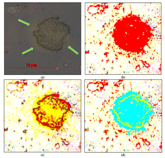
Figure 11.
Thresholding of a particle surrounded by a shade: (a) original image, green arrows show the surrounding shade; (b) mineral thresholding; (c) border thresholding; (d) “Threshold” view, showing border as yellow.
Attempting to threshold this particle will unavoidably select a significant portion of the surrounding area as shown in Figure 11b. To significantly improve the quality of non-opaque mineral identification in this particular case, the area determined by thresholding needs to be brought closer to the visible particle boundary. Another algorithm, code-named “reduction to border” (described as Algorithm S3 in Supplementary Material and including workflow steps D and E in Figure 3), can be employed for that purpose, activated via the “Use borders” checkbox (Figure 12) and corresponding controls.
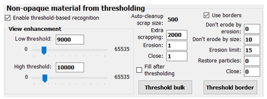
Figure 12.
Threshold-based identification frame with the “Use borders” section enabled.
First of all, in order to perform the “reduction to border” operation, the bulk of the particle and its border have to be thresholded. The latter (step D in Figure 3) is performed by selecting the “Threshold border” button (see Figure 12). An example of such a thresholding is demonstrated in Figure 11c. Particle borders normally correspond to the darkest areas in the enhanced view and thus can be thresholded reliably to a certain extent. It should be noted though, that in the chosen example, the visible border has significant breaks, so identification of the particle based on the border alone may be problematic. The thresholded border will also appear in yellow in the “Threshold” view of the form, as shown in Figure 11d. In this view, similar to what was shown in Figure 10, the identified particle area, after the cleanup and close operations were performed, is shown in cyan and the cleaned-up areas are shown in red. It is obvious that due to the “shade” underneath the epoxy, the particle area was overestimated and is significantly outside its actual borders.
The algorithm will now attempt to remove the wrongly identified mineral area present outside the optically discontinuous particle border, while retaining identified material present inside the border. The “reduction to border” operation itself is controlled by the “Erosion limit” parameter. The particle area is subjected to erosion operations according to the operator set limit; however, the particle matter only is eroded until it reaches the particle border. The erosion can only propagate within particle borders where there are breaks in the border. Good border identification combined with an appropriately chosen erosion limit can ensure that the effect of such over-erosion inside particles is relatively small compared to the improved identification of the particle.
Figure 13 provides examples of the effect of different erosion limits on particle identification. The minimal erosion limit is 1, as erosion is the essential part of the “reduction to border” operation. The particle area in Figure 13a, obtained with erosion 1, is nearly the same as the original thresholding result (cyan in Figure 11d). The area in Figure 13b, with erosion 5, is still mostly outside of the real particle, but the top-right part of it is now close to real (refer to Figure 11a). Note that it will not change with subsequent erosions because the identified border there is reasonably solid and will “resist” the erosion according to the algorithm. The particle in Figure 13c, after erosion 10, is reasonably close to the real object and represents what the image analysis is aimed at. The excessive erosion of 15 in Figure 13d starts to remove parts of the actual particle where borders are the most indistinct.
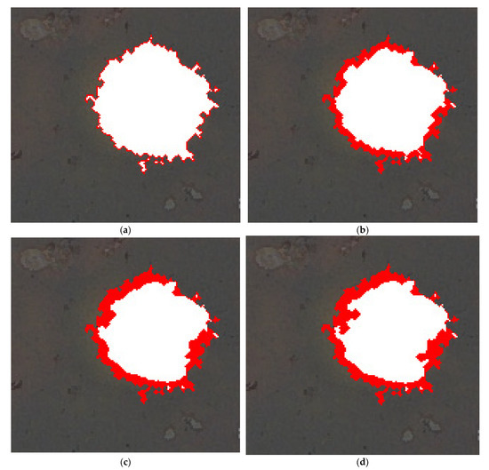
Figure 13.
Results of applying different erosion limits to the particle from Figure 11a: (a) 1; (b) 5; (c) 10; (d) 15. Red colour represents the identified particle area outline in the absence of border-based erosion.
The algorithm described above is based on erosion, so particular care should be taken about the cases where the erosion would have a detrimental effect. In particular, non-selective application of the algorithm to smaller objects and/or objects without a distinct actual border inside is likely to either completely eliminate or significantly distort them. Thus, a number of steps have been taken to prevent that from happening and to only apply the operation to larger non-opaque objects. It is assumed that the non-opaque mineral map is already meaningful at this stage of analysis, and any objects in it, even small ones, should be reported as non-opaque particles or grains; otherwise, they would have been removed during non-opaque map cleanup as discussed in the previous section.
First of all, very small objects are extremely unlikely to contain within them a distinct and mostly continuous border suitable for a “reduction to border” operation. Erosion operations performed on particles with a fragmented border would result in removal of most of the particle matter, whether truly or falsely identified by thresholding, in such particles. Thus, particles below a certain area size can be fully exempted from the “reduction to borders” operation. The size limit can be defined by susceptibility to erosion or by the actual area. In the first case, prior to applying “reduction to borders” the thresholded map is subjected to erosion to the value set by the “Don’t erode by erosion” parameter (Figure 12). Any particles that would be fully destroyed by such an erosion procedure are identified and preserved. In a similar manner, the thresholded map is also scrapped by area, according to the “Don’t erode by size” parameter (Figure 12). These particles are preserved too and the “reduction to border” operation is not performed on them.
The map subjected to “reduction to borders” is therefore the original thresholded and cleaned-up map with the exception of any areas preserved by the “don’t erode” operations described above. It must be noted that the remaining objects, even if they are reasonably large, may also be fully or partially lost to erosion, especially if their borders were significantly underestimated. To prevent such an excessive loss from happening, the erosion is applied selectively to each object. The number of erosions for each individual object is adjusted based on the object width in pixels; the maximum number of iterations cannot exceed ¼ of the particle width which, keeping in mind that every single erosion step consumes 2 pixels of width, means that the particle will retain at least half of its width (in the worst-case scenario of no border at all to stop erosion) at the end of the procedure.
Another parameter preventing the possible negative effect of erosion is “Restore particles” (Figure 12). It addresses the possibility that non-opaque grains that belong to larger particles can be detached from them as a result of erosion. For the non-opaque grain, the border visibility along its connection with the rest of the particle can be very low. Erosion during “reduction to border” will then shrink the non-opaque matter in that area, resulting in a loss of connection between the grain and the rest of the particle. To prevent that from happening, both the non-opaque map and the known particle map can be dilated according to the “Restore particles” parameter, and the intersection of those dilated maps will be added to the particle border, preventing the erosion along the connection. This parameter should be kept reasonably low to prevent establishing false connections between otherwise unconnected objects.
Finally, “Close” operations (Figure 12) can be applied to the resulting map if erosion results in unexpected gaps in particles. For example, applying Close = 3 to the over-eroded particle in Figure 13d will make it look more like the reasonably good result in Figure 13c. An appropriate choice of erosion and close parameters enables the best identification of non-opaque material during “reduction to borders”, which corresponds to workflow step E in Figure 3. It should be noted that the examples in this paper were necessarily restricted to individual particles or small groups of particles. At the same time, threshold-based non-opaque identification, performed by Mineral5 in automated mode over multiple images containing hundreds of particles, is aimed not at achieving perfect results for individual particles, which is typically not possible due to the boundary thickness variability. Rather, it aims to produce reasonable results for most non-opaque objects present without introducing a significant amount of false identifications, and this is what the operator’s efforts in analysis profile development and verification are typically aimed at.
4. Combining Two Identification Algorithms
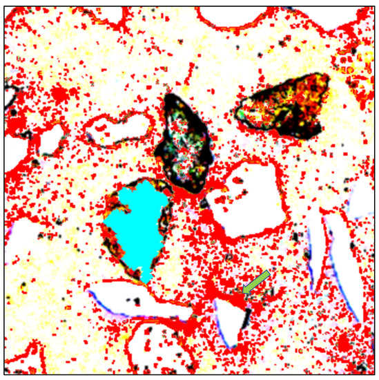
For the best possible results, Mineral5 allows for a combination of both border-based [36] and threshold-based identifications of non-opaque minerals (see Figure 3). In the most typical scenario, the results of both algorithms are combined. Figure 14 shows the final mineral identification for the image from Figure 2, where particles A and B with strong borders were identified using the border-based method, and particle C was identified by the thresholding method described in this paper (see also Figure 8).
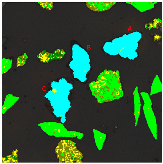
Figure 14.
Final mineral identification for particles from Figure 2 (light green—vitreous goethite, brown—ochreous goethite, dark green—kaolinite, cyan—quartz, yellow—porosity). Quartz identification is border-based for particles A and B, threshold-based for particle C.
Another possible option for combining the results of the two identification algorithms, also implemented in Mineral5, is using threshold-based identification to assign distinct areas identified by the border-based algorithm, to either epoxy or non-opaque minerals. As described by Poliakov and Donskoi [36], the border-based method, particularly in the presence of multiple touching non-opaque particles and/or scratches in the epoxy (which can be falsely identified as particle borders), can sometimes be a very complex task for a software algorithm. Therefore, if non-opaque matter can be segmented by thresholding, even very coarsely, such a thresholding can be used to reliably assign problematic areas within borders (actual or falsely identified) to either non-opaque mineral or epoxy.
5. Conclusions
This article presents an algorithm for performing non-opaque mineral segmentation in optical image analysis by thresholding, which was not previously considered feasible for some minerals, e.g., quartz. This recently developed procedure now enables such segmentation to be performed standalone or, if necessary, in combination with the previously reported border-based method. The procedure includes three major steps. The first one is the adjustment of epoxy resin reflectivity by adding excessive amounts of Epodye, if the initial reflectivity of epoxy resin is the same or very similar to that of the target non-opaque mineral. The second step includes segmentation of all opaque minerals and exclusion of their areas from consideration prior to non-opaque minerals segmentation, in order to reduce misidentifications. The final step is utilisation of enhanced thresholding followed by specific procedures reducing or fully eliminating misidentifications in the epoxy area.
The enhanced thresholding begins by adjusting the image to extend a narrow reflectivity range, encompassing that of both non-opaque minerals and epoxy resin, into a much wider range, significantly increasing the visibility of the mineral. Further application of “fill” and/or “close” operations allows identified areas of the non-opaque mineral to be solidified. Noise removal by scrapping and erosion then only leaves genuine non-opaque objects. In the presence of significant under-epoxy “shades”, a “reduction to borders” operation can be performed to further improve identification. By identifying the visible part of particle borders and then performing selective erosion, it can be ensured that the segmented non-opaque areas are within actual particle boundaries. The algorithm options also ensure that non-opaque grains are not detached by erosion from particles with complex mineralogy, and that smaller non-opaque objects are preserved and not fully lost to erosion.
Comprehensive thresholding of non-opaque minerals described in the paper is a relatively simple option compared with deep learning techniques. In combination with border-based discrimination of non-opaque minerals previously described [36], it allows reliable segmentation of non-opaque minerals in reflected light optical microscopy.
Supplementary Materials
The following supporting information can be downloaded at: https://www.mdpi.com/article/10.3390/min13030350/s1, Algorithm S1: Image view enhancement; Algorithm S2: Produce map of non-opaque mineral; Algorithm S3: Improve map of non-opaque mineral by “reduction to border”.
Author Contributions
Conceptualisation, A.P. and E.D.; methodology, A.P. and E.D.; software, A.P. and E.D.; writing—original draft, A.P. and E.D.; writing—review and editing, A.P. and E.D.; visualisation, A.P.; project administration, E.D. All authors have read and agreed to the published version of the manuscript.
Funding
This research received no external funding.
Data Availability Statement
Data sharing not applicable.
Acknowledgments
The authors wish to thank CSIRO Carbon Steel Materials group staff for their support during this work. We would like to acknowledge Mike Peterson for valuable suggestions and correction of this article. We would also like to express our gratitude to the internal and external reviewers for useful corrections and comments.
Conflicts of Interest
The authors declare no conflict of interest.
References
- Chopard, A.; Marion, P.; Mermillod-Blondin, R.; Plante, B.; Benzaazoua, M. Environmental impact of mine exploitation: An early predictive methodology based on ore mineralogy and contaminant speciation. Minerals 2019, 9, 397. [Google Scholar] [CrossRef]
- Makvandi, S.; Pagé, P.; Tremblay, J.; Girard, R. Exploration for platinum-group minerals in till: A new approach to the recovery, counting, mineral identification and chemical characterization. Minerals 2021, 11, 264. [Google Scholar] [CrossRef]
- Donskoi, E.; Suthers, S.P.; Campbell, J.J.; Raynlyn, T.; Clout, J.M.F. Prediction of hydrocyclone performance in iron ore beneficiation using texture classification. In Proceedings of the XXIII International Mineral Processing Congress, Istanbul, Turkey, 3–8 September 2006; pp. 1897–1902. [Google Scholar]
- Donskoi, E.; Holmes, R.J.; Manuel, J.R.; Campbell, J.J.; Poliakov, A.; Suthers, S.P.; Raynlyn, T. Utilization of Iron Ore Texture Information for Prediction of Downstream Process Performance. In Proceedings of the 9th International Congress for Applied Mineralogy Brisbane, Australia, 8–10 September 2008; pp. 687–693. [Google Scholar]
- Donskoi, E.; Manuel, J.R.; Lu, L.; Holmes, R.J.; Poliakov, A.; Raynlyn, T.D. Importance of textural information in mathematical modelling of iron ore fines sintering performance. Miner. Process Extr. M 2018, 127, 103–114. [Google Scholar] [CrossRef]
- König, U.; Verryn, S.M.C. Heavy mineral sands mining and downstream processing: Value of mineralogical monitoring using XRD. Minerals 2021, 11, 1253. [Google Scholar] [CrossRef]
- König, U. Application of X-ray diffraction to iron ores- potential implications for grade control and downstream processing. In Proceedings of the Iron Ore 2013, Perth, Australia, 12–14 August 2013; pp. 275–280. [Google Scholar]
- Barbery, G. Liberation 1, 2, 3: Theoretical analysis of the effect of space dimension on mineral liberation by size reduction. Miner. Eng. 1992, 5, 123–141. [Google Scholar] [CrossRef]
- Schneider, C.L. Measurement and Calculation of Liberation in Continuous Milling Circuits. Ph.D. Thesis, University of Utah, Salt Lake City, UT, USA, 1995. [Google Scholar]
- Poliakov, A.; Donskoi, E. Separation of touching particles in optical image analysis of iron ores and its effect on textural and liberation characterization. Eur. J. Miner. 2019, 31, 485–505. [Google Scholar] [CrossRef]
- Chescoe, D.C.; Goodhew, P.J. The Operation of Transmission and Scanning Electron Microscopes, 1st ed.; Oxford University Press: Oxford, UK, 1990; p. 20. [Google Scholar]
- Gottlieb, P.; Wilkie, G.; Sutherland, D.; Ho-Tun, E.; Suthers, S.; Perera, K.; Jenkins, B.; Spencer, S.; Butcher, A.; Rayner, J. Using quantitative electron microscopy for process mineralogy applications. JOM 2000, 52, 24–25. [Google Scholar] [CrossRef]
- Gu, Y. Automated scanning electron microscope based mineral liberation analysis. J. Miner. Mater. Charact. Eng. 2003, 2, 33–41. [Google Scholar]
- Goodall, W.R.; Scales, J.J.; Butcher, A. The use of QEMSCAN and diagnostic leaching in the characterisation of visible gold in complex ores. Miner. Eng. 2005, 18, 877–886. [Google Scholar] [CrossRef]
- Maddren, J.; Ly, C.V.; Suthers, S.P.; Butcher, A.R.; Trudu, A.G.; Botha, P.W.S.K. A new approach to ore characterisation using automated quantitative mineral analysis. In Proceedings of the Iron Ore 2007, Perth, Australia, 20–22 August 2007; pp. 131–132. [Google Scholar]
- De Castro, B.; Benzaazoua, M.; Chopard, A.; Plante, B. Automated mineralogical characterization using optical microscopy: Review and recommendations. Miner. Eng. 2022, 189, 107896. [Google Scholar] [CrossRef]
- Santoro, L.; Lezzerini, M.; Aquino, A.; Domenighini, G.; Pagnotta, S. A Novel Method for Evaluation of Ore Minerals Based on Optical Microscopy and Image Analysis: Preliminary Results. Minerals 2022, 12, 1348. [Google Scholar] [CrossRef]
- Pirard, E.; Lebichot, S. Image analysis of iron oxides under the optical microscope. In Applied Mineralogy: Developments in Science and Technology; ICAM: Sao Paulo, Brazil, 2004; pp. 153–156. [Google Scholar]
- Pirard, E.; Lebichot, S.; Krier, W. Particle texture analysis using polarized light imaging and grey level intercepts. Int. J. Miner. Process 2007, 84, 299–309. [Google Scholar] [CrossRef]
- Gomes, O.D.M.; Paciornik, S. Iron ore quantitative characterization through reflected light-scanning electron co-site microscopy. In Proceedings of the Ninth International Congress on Applied Mineralogy, Brisbane, Australia, 8–10 September 2008; pp. 699–702. [Google Scholar]
- Donskoi, E.; Poliakov, A.; Manuel, J.R. Automated Optical Image Analysis of Natural and Sintered Iron Ore. In Iron Ore: Mineralogy, Processing and Environmental Sustainability; Lu, L., Ed.; Elsevier: Cambridge, UK, 2015; pp. 101–159. [Google Scholar]
- Donskoi, E.; Manuel, J.R.; Austin, P.; Poliakov, A.; Peterson, M.J.; Hapugoda, S. Comparative Study of Iron Ore Characterisation by Optical Image Analysis and QEMSCANTM. In Proceedings of the Iron Ore 2011, Perth, Australia, 5–7 April 2011; pp. 213–222. [Google Scholar]
- Higgins, M.D. Imaging birefringent minerals without extinction using circularly polarized light. Can. Miner. 2010, 48, 231–235. [Google Scholar] [CrossRef]
- Gomes, O.D.M.; Paciornik, S.; Iglesias, J.C.A. A simple methodology for identifying hematite grains under polarized reflected light microscopy. In Proceedings of the 17th International Conference on Systems, Signals and Image Processing—IWSSIP 2010, Rio de Janeiro, Brazil, 17–19 June 2010; 2010; pp. 428–431. [Google Scholar]
- Iglesias, J.C.A.; Gomes, O.D.M.; Paciornik, S. Automatic recognition of hematite grains under polarized reflected light microscopy through image analysis. Miner. Eng. 2011, 24, 1264–1270. [Google Scholar] [CrossRef]
- Donskoi, E.; Poliakov, A.; Vining, K. Structural and Textural Characterization of Coke with Optical Image Analysis Software. In Proceedings of the AISTech 2019 Iron and Steel Technology Conference and Exposition, Pittsburgh, PA, USA, 6–9 June 2019; pp. 237–254. [Google Scholar]
- Launeau, P.; Cruden, A.R.; Bouchez, J.L. Mineral recognition in digital images of rocks: A new approach using multichannel classification. Can. Mineral. 1994, 32, 919–933. [Google Scholar]
- Neumann, R.; Stanley, C.J. Specular reflectance data for quartz and some epoxy resins—Implications for digital image analysis based on reflected light optical microscopy. In Proceedings of the Ninth International Congress for Applied Mineralogy, Brisbane, Australia, 8–10 September 2008; pp. 703–705. [Google Scholar]
- Lane, G.R.; Martin, C.; Pirard, E. Techniques and applications for predictive metallurgy and ore characterization using optical image analysis. Miner. Eng. 2008, 21, 568–577. [Google Scholar] [CrossRef]
- Donskoi, E.; Raynlyn, T.D.; Poliakov, A. Image Analysis Estimation of Iron Ore Particle Segregation in Epoxy Blocks. Miner. Eng. 2018, 120, 102–109. [Google Scholar] [CrossRef]
- Iglesias, J.C.A.; Santos, R.B.M.; Paciornik, S. Deep learning discrimination of quartz and resin in optical microscopy images of minerals. Miner. Eng. 2019, 138, 79–85. [Google Scholar] [CrossRef]
- Filippo, M.P.; Gomes, O.D.M.; da Costa, G.A.O.P.; Mota, G.L.A. Deep learning semantic segmentation of opaque and non-opaque minerals from epoxy resin in reflected light microscopy images. Miner. Eng. 2021, 170, 107007. [Google Scholar] [CrossRef]
- Delbem, I.D. Automated Iron Ores Characterisation via Reflected Light Optical Microscope. Ph.D. Thesis, Universidade Federal de Minas Gerais, Belo Horizonte, Brazil, 2014; p. 122. (In Portuguese). [Google Scholar]
- Delbem, I.D.; Galéry, R.; Brandão, P.R.G.; Peres, A.E.C. Semi-automated iron ore characterisation based on optical microscope analysis: Quartz/resin classification. Miner. Eng. 2015, 82, 2–13. [Google Scholar] [CrossRef]
- Gonzalez, R.C.; Woods, R.E. Digital Image Processing, 3rd ed.; Prentice Hall: Hoboken, NJ, USA, 2008; p. 624. [Google Scholar]
- Poliakov, A.; Donskoi, E. Automated relief-based discrimination of non-opaque minerals in optical image analysis. Miner. Eng. 2014, 55, 111–124. [Google Scholar] [CrossRef]
- Donskoi, E.; Poliakov, A.; Vining, K. Transformation of Automated Optical Image Analysis Software Mineral4/Recognition4 to Mineral5/Recognition5. In Proceedings of the Iron Ore 2021, Perth, Australia, 8–10 November 2021; pp. 374–390. [Google Scholar]
- Iglesias, J.C.A.; Augusto, K.S.; Gomes, O.D.M.; Domongues, A.L.A.; Viera, M.B.; Casagrande, C.; Paciornik, S. Automatic characterization of iron ore by digital microscopy and image analysis. J. Mater. Res. Technol. 2018, 7, 376–380. [Google Scholar] [CrossRef]
- Donskoi, E.; Manuel, J.R.; Hapugoda, S.; Poliakov, A.; Raynlyn, T.; Austin, P.; Peterson, M. Automated optical image analysis of goethitic iron ores. Miner. Process Extr. M 2022, 131, 14–24. [Google Scholar] [CrossRef]
- Donskoi, E.; Hapugoda, S.; Manuel, J.R.; Poliakov, A.; Peterson, M.J.; Mali, H.; Bückner, B.; Honeyands, T.; Pownceby, M.I. Automated Optical Image Analysis of Iron Ore Sinter. Minerals 2021, 11, 562. [Google Scholar] [CrossRef]
- Donskoi, E.; Poliakov, A. Advances in Optical Image Analysis Textural Segmentation in Ironmaking. Appl. Sci. 2020, 10, 6242. [Google Scholar] [CrossRef]
- Otsu, N. Threshold selection method from gray-level histograms. IEEE Trans. Syst. Man Cybern. 1979, 9, 62–66. [Google Scholar] [CrossRef]


Disclaimer/Publisher’s Note: The statements, opinions and data contained in all publications are solely those of the individual author(s) and contributor(s) and not of MDPI and/or the editor(s). MDPI and/or the editor(s) disclaim responsibility for any injury to people or property resulting from any ideas, methods, instructions or products referred to in the content. |
© 2023 by the authors. Licensee MDPI, Basel, Switzerland. This article is an open access article distributed under the terms and conditions of the Creative Commons Attribution (CC BY) license (https://creativecommons.org/licenses/by/4.0/).