
Denoising Marine Controlled Source Electromagnetic Data Based on Dictionary Learning


Abstract
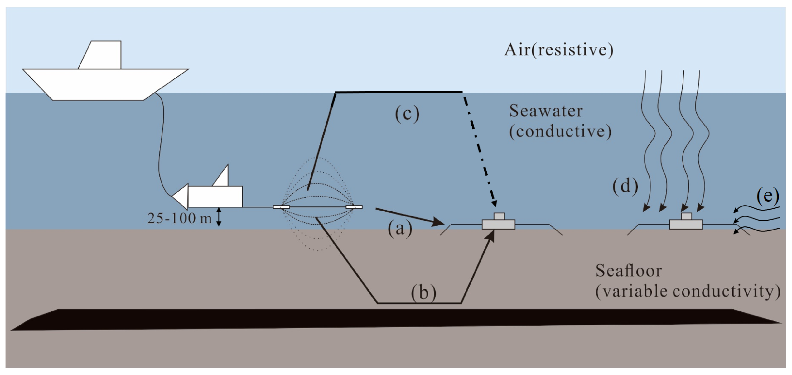
:1. Introduction
- (1)
- Dipole vibrations. The vibration of receiver arm will induce a voltage, whose magnitude is comparable to the target signal [5].
- (2)
- Seafloor currents. Seafloor currents will induce voltages that always have a low frequency closely related to the currents [6].
- (3)
- Natural electromagnetic field variations. The changes of natural electromagnetic field can influence the recorded signal, such as magnetotelluric.
- (4)
- Internal electrode and amplifier noise. This noise comes from the internal part of the instrument.
- (5)
- Air waves. Air waves can seriously affect the data quality in shallow water exploration. Its influence will be weakened with the increase of seawater depth. Despite the disagreement whether air waves are noise or not, many scholars still try to remove it [7].
2. Theory and Methodology
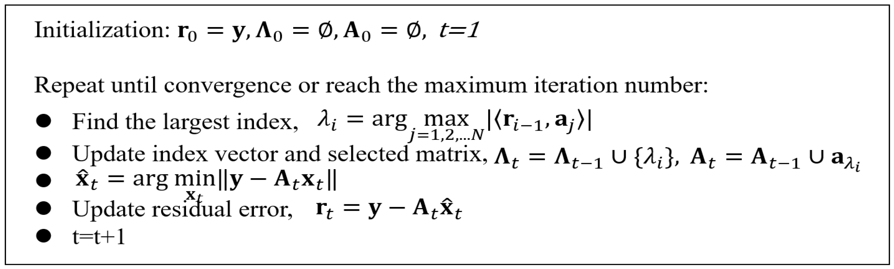
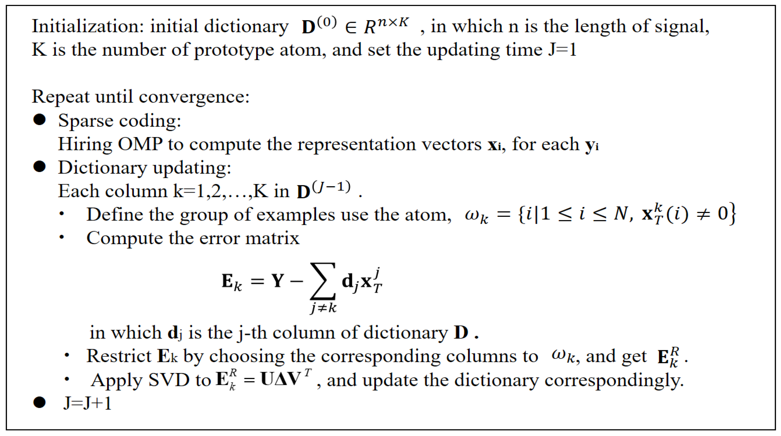
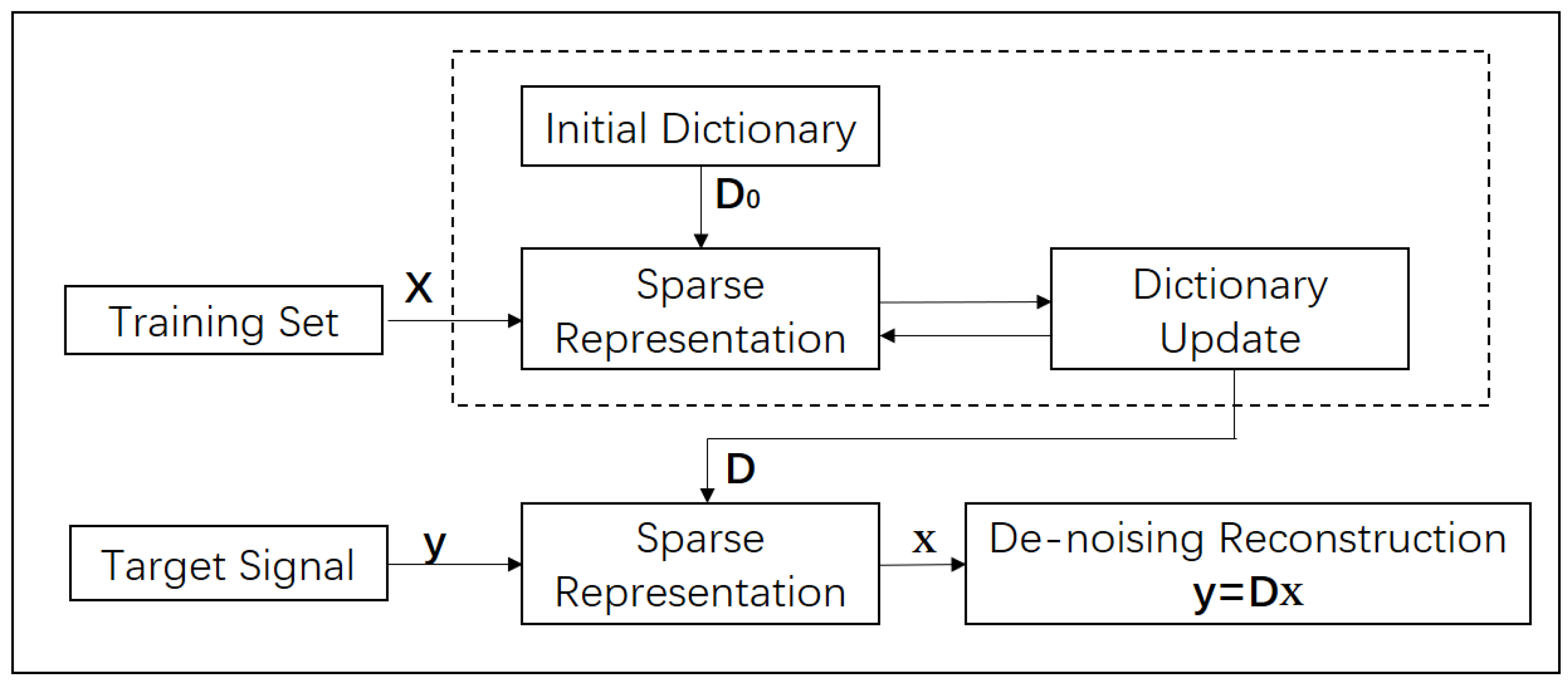
2.1. Dictionary Learning Based on K-SVD Algorithm
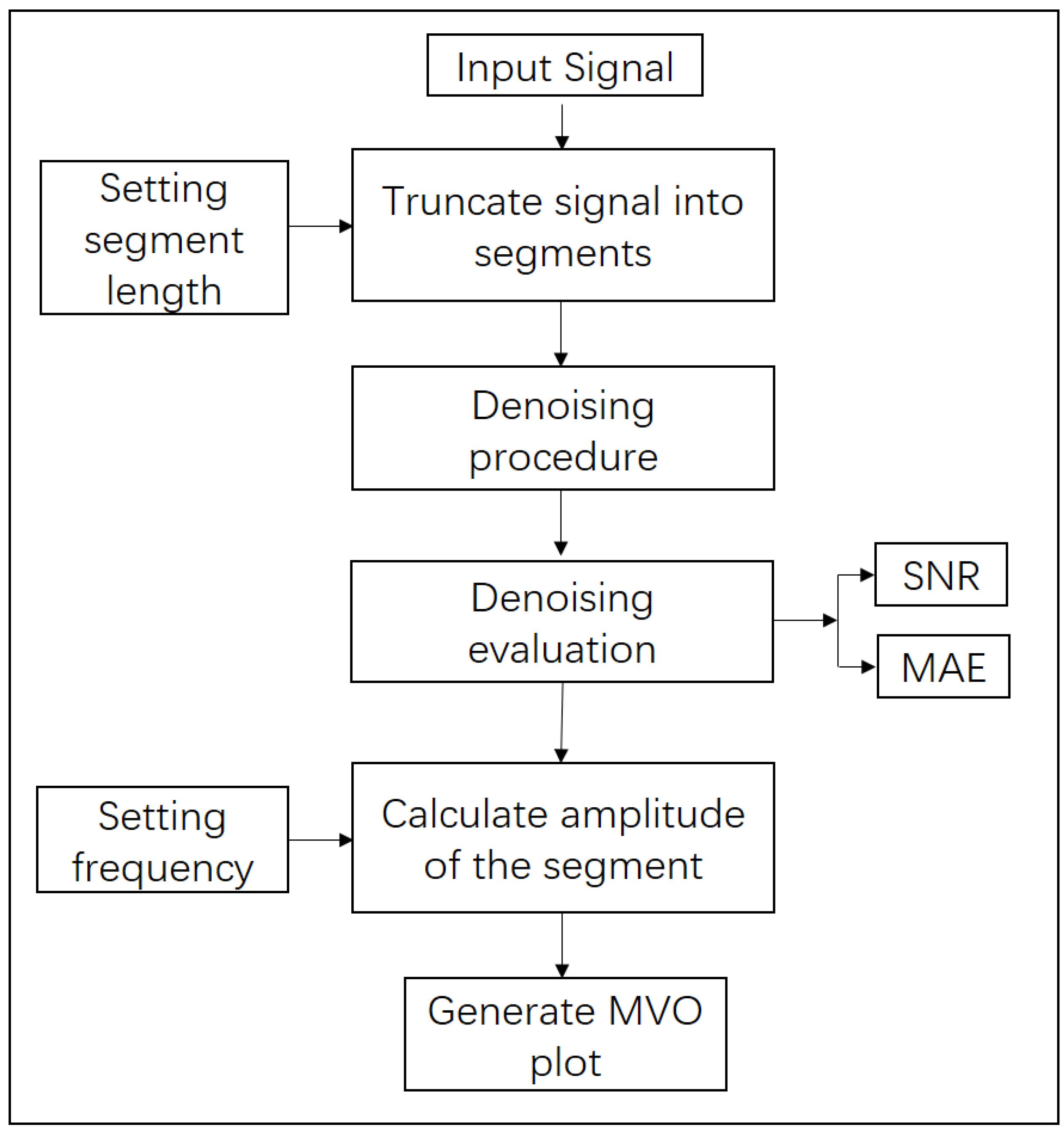
2.2. Denoising Flow of the Proposed Algorithm
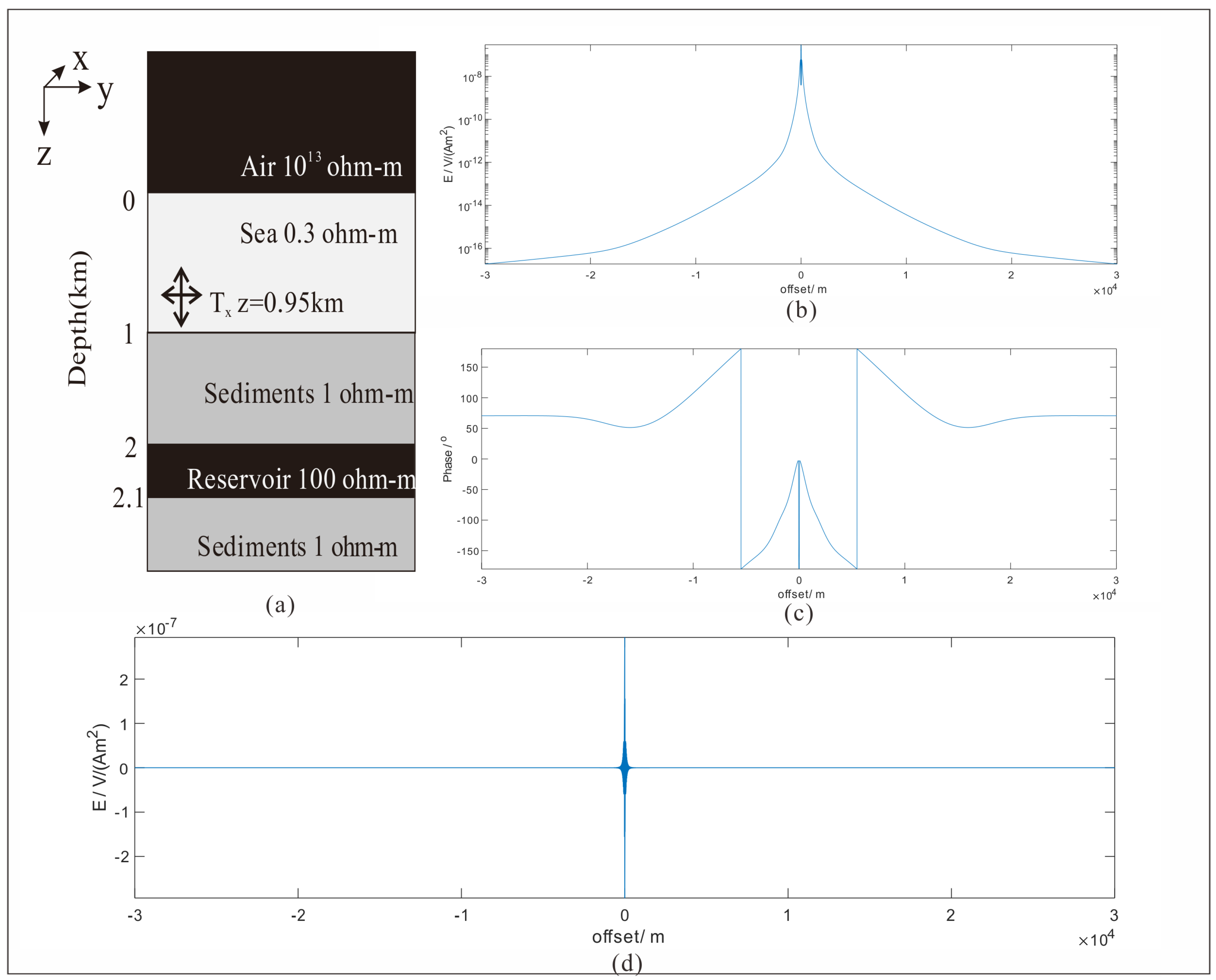
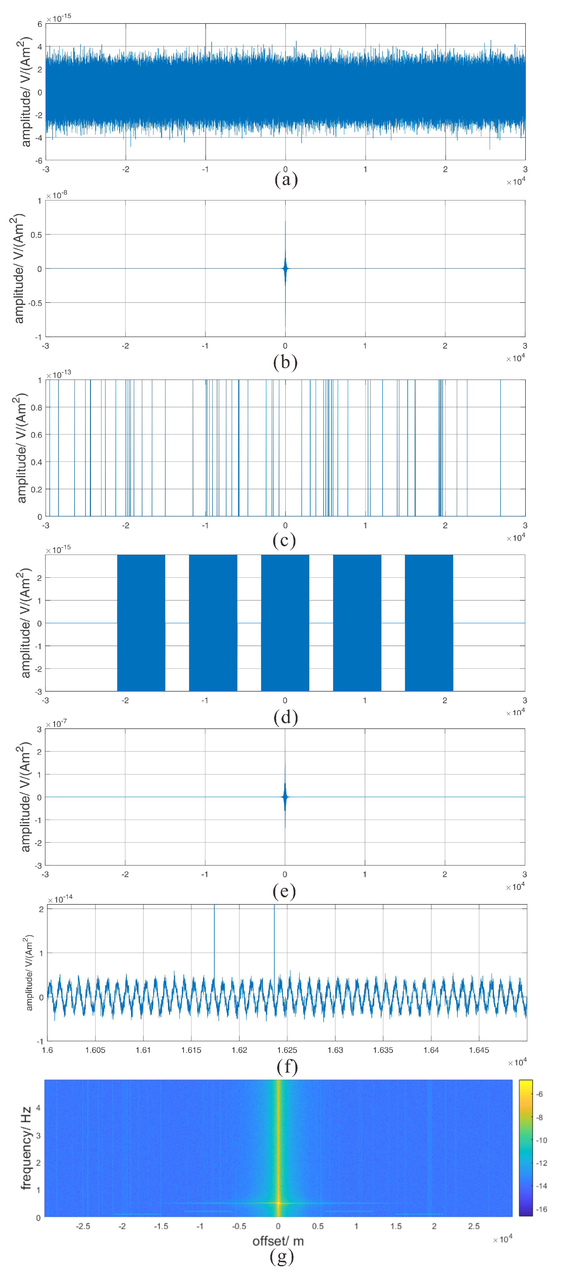
3. Synthetic Data Examples
- (1)
- Random noise. Magnitudes are integer multiples of the noise floor V/(Am2), and the average value is zero [24].
- (2)
- Internal noise. This kind of noise originates from the circuitry of the equipment, and the magnitude is set as of clear signal to simulate the amplifier noise [13].
- (3)
- Impulse noise. Thirty positive impulses with the magnitude V/(Am2) are added randomly to the signal to simulate the accidental interferences.
- (4)
- Low frequency noise. The motion of seawater is complex and so is the noise caused by this movement. The noise has multiple frequencies surrounding low frequency. To simply the research, we use five low frequency sine signals with the frequency 0.01, 0.02, 0.03, 0.04 and 0.05 Hz separately to simulate the seawater motion influence.
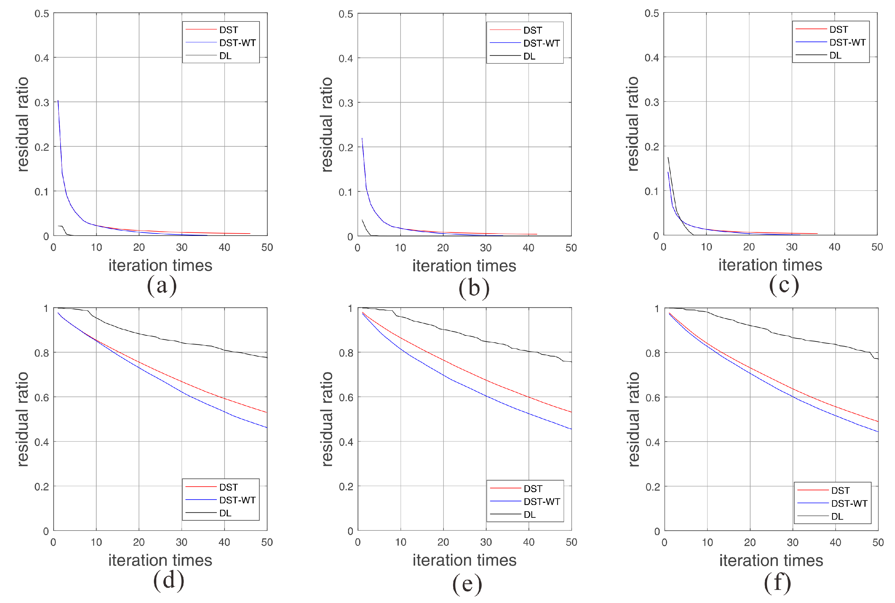
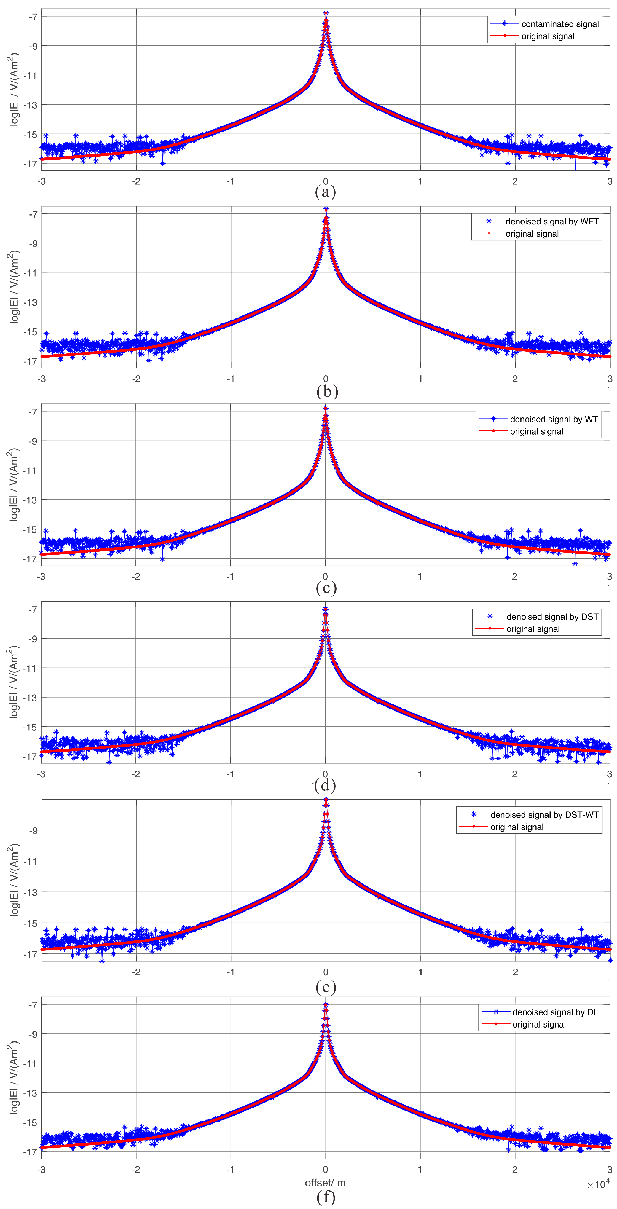
3.1. Numerical Experiment I
3.2. Numerical Experiment II
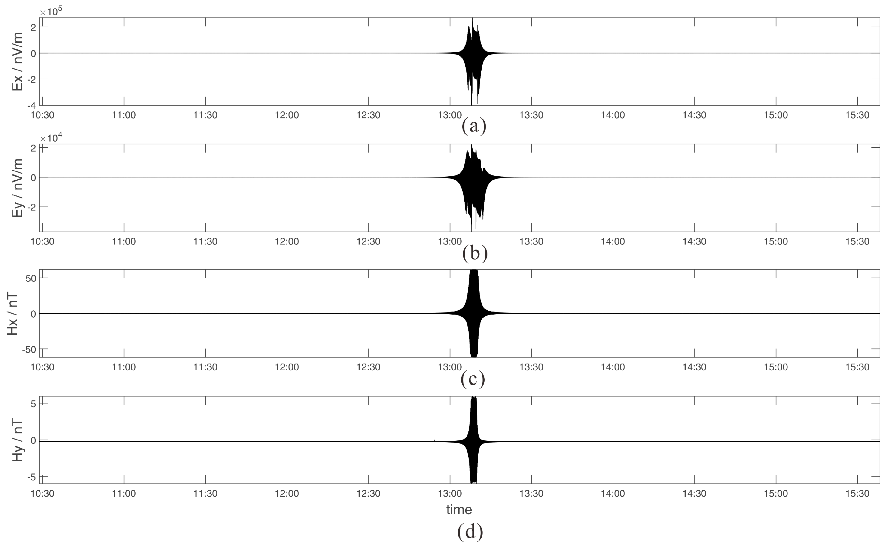
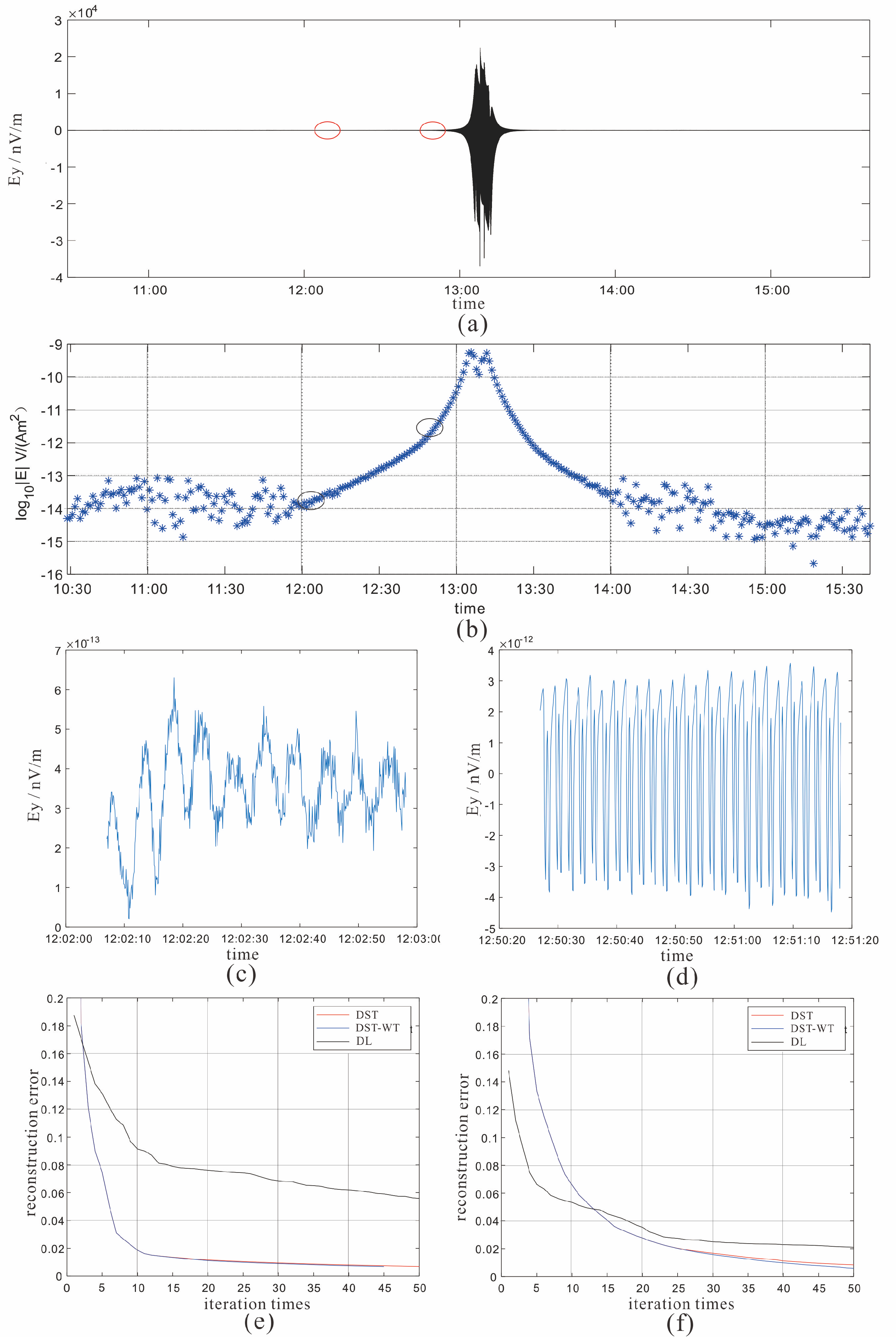
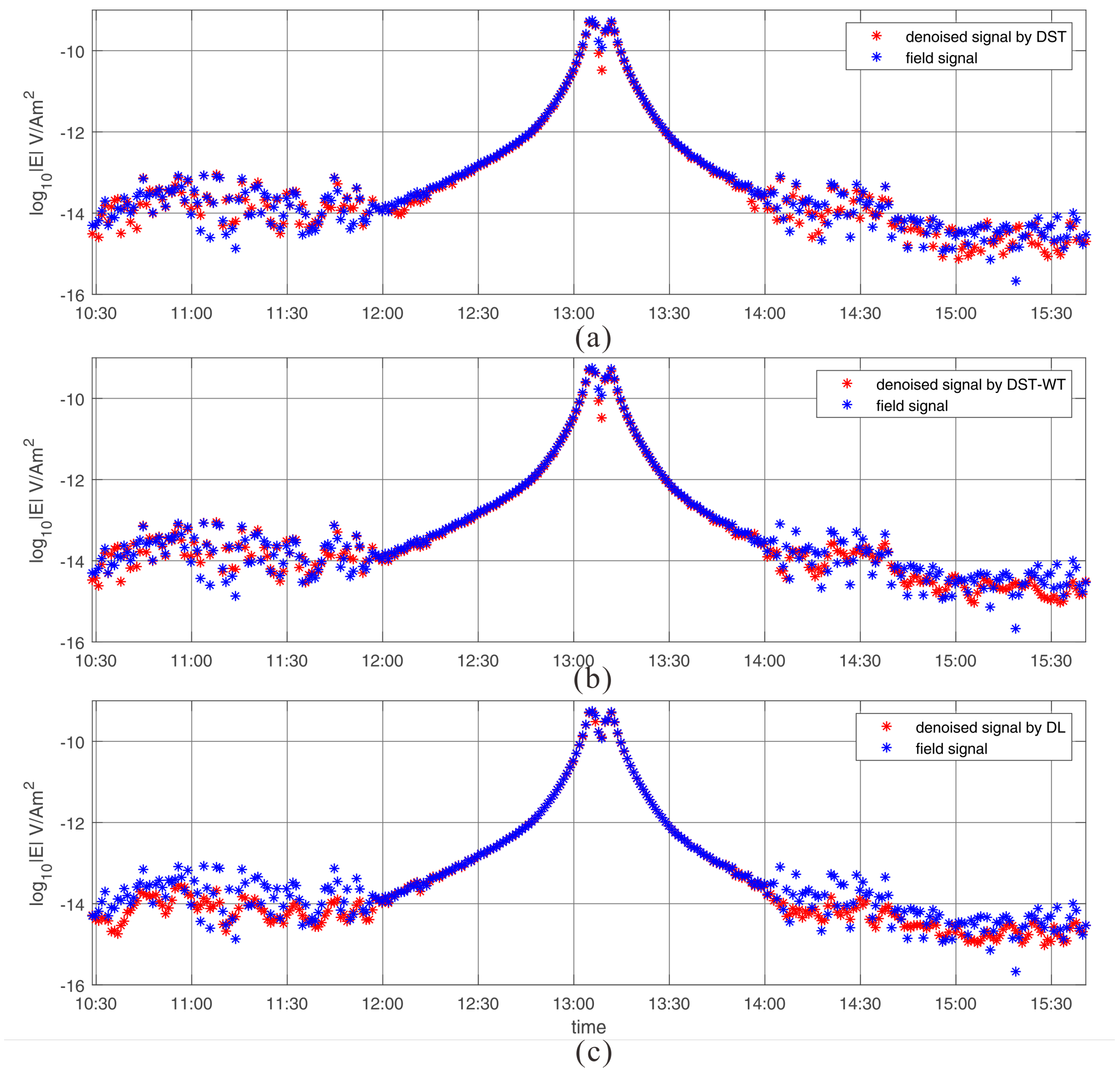
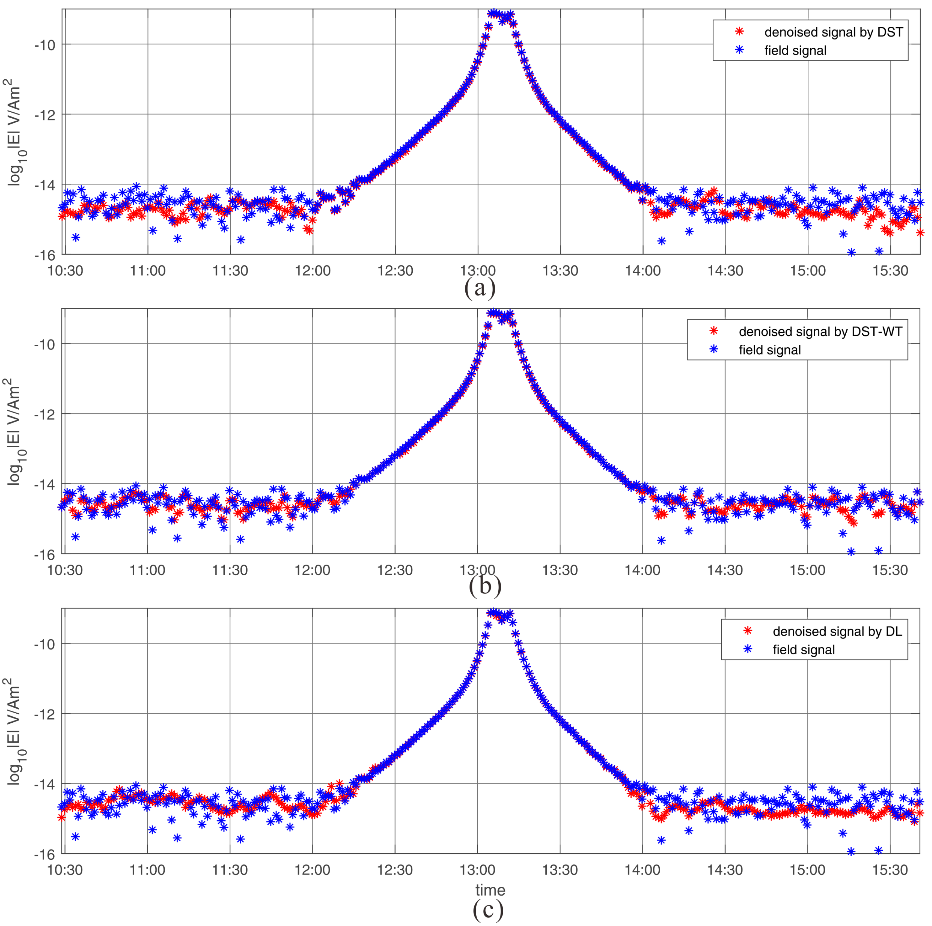
4. Real Data Application
5. Conclusions
Author Contributions
Funding
Data Availability Statement
Acknowledgments
Conflicts of Interest
Abbreviations
| CSEM | controlled source electromagnetic |
| WFT | windowed Fourier transform |
| WT | wavelet transform |
| DST | discrete sine transform |
| OMP | orthogonal matching pursuit |
| target signal | |
| sparse coefficients vector | |
| dictionary | |
| error | |
| the calculated sparse coefficients vector | |
| residual for the ith iteration | |
| index set for the column number for ith iteration | |
| column set for ith iteration |
References
- Constable, S.; Srnka, L.J. An introduction to marine controlled-source electromagnetic methods for hydrocarbon exploration. Geophysics 2007, 72, WA3–WA12. [Google Scholar] [CrossRef]
- Peng, R.; Hu, X.; Chen, B.; Li, J. 3-D marine controlled-source electromagnetic modeling in electrically anisotropic formations using scattered scalar–vector potentials. IEEE Geosci. Remote Sens. Lett. 2018, 15, 1500–1504. [Google Scholar] [CrossRef]
- Constable, S. Ten years of marine CSEM for hydrocarbon exploration. Geophysics 2010, 75, 75A67–75A81. [Google Scholar] [CrossRef] [Green Version]
- Pethick, A.M. Multidimensional Computation and Visualisation for Marine Controlled Source Electromagnetic Methods. Ph.D. Thesis, Curtin University, Perth, WA, Australia, 2013. [Google Scholar]
- Liu, N. Preprocessing and Research of Denoising Methods for Marine Controlled Source Electromagnetic Data. Ph.D. Thesis, Jilin University, Changchun, China, 2015. (In Chinese). [Google Scholar]
- Zili, Z. Theory Research and Application of Ocean Electromagnetic Field. Ph.D. Thesis, China University of Geosciences, Wuhan, China, 2009. [Google Scholar]
- Yin, C.; Liu, Y.; Weng, A.; Jia, D.; Ben, F. Research on marine controlled-source electromagnetic method airwave. J. Jilin Univ. (Earth Sci. Ed.) 2012, 42, 1506–1520. [Google Scholar]
- Behrens, J.P. The Detection of Electrical Anisotropy in 35 Ma Pacific Lithosphere: Results from a Marine Controlled-Source Electromagnetic Survey and Implications for Hydration of the Upper Mantle; University of California: San Diego, CA, USA, 2005. [Google Scholar]
- Myer, D.; Constable, S.; Key, K. Broad-band waveforms and robust processing for marine CSEM surveys. Geophys. J. Int. 2011, 184, 689–698. [Google Scholar] [CrossRef] [Green Version]
- Hsu, S.K.; Chiang, C.W.; Evans, R.L.; Chen, C.S.; Chiu, S.D.; Ma, Y.F.; Chen, S.C.; Tsai, C.H.; Lin, S.S.; Wang, Y. Marine controlled source electromagnetic method used for the gas hydrate investigation in the offshore area of SW Taiwan. J. Asian Earth Sci. 2014, 92, 224–232. [Google Scholar] [CrossRef]
- Xin, L.; Wen-bo, W.; Jian-en, J. Study on improving MCSEM signal-to-noise ratio. Prog. Geophys. 2009, 24, 1047–1050. [Google Scholar]
- Li, Z. Study on Marine Controlled-Source Electromagnetic Data De-Noising Based on Adaptive Filtering Method. Ph.D. Thesis, China University of Geosciences, Wuhan, China, 2017. [Google Scholar]
- Zhang, P.; Deng, M.; Jing, J.; Chen, K. Marine controlled-source electromagnetic method data de-noising based on compressive sensing. J. Appl. Geophys. 2020, 177, 104011. [Google Scholar] [CrossRef]
- Li, G.; Liu, X.; Tang, J.; Li, J.; Ren, Z.; Chen, C. De-noising low-frequency magnetotelluric data using mathematical morphology filtering and sparse representation. J. Appl. Geophys. 2020, 172, 103919. [Google Scholar] [CrossRef]
- Xue, S.Y.; Yin, C.C.; Su, Y.; Liu, Y.H.; Wang, Y.; Liu, C.H.; Xiong, B.; Sun, H.F. Airborne electromagnetic data denoising based on dictionary learning. Appl. Geophys. 2020, 17, 306–313. [Google Scholar] [CrossRef]
- Tang, J.; Li, G.; Zhou, C.; Ren, Z.; Xiao, X.; Liu, Z.j. Denoising AMT data based on dictionary learning. Chin. J. Geophys. 2018, 61, 3835–3850. [Google Scholar]
- Ma, J.; Plonka, G. The curvelet transform. IEEE Signal Process. Mag. 2010, 27, 118–133. [Google Scholar] [CrossRef]
- Zhang, P.; Pan, X.; Guo, Z.; Ge, Z.; Liu, J. Application of dictionary learning in marine CSEM denoising. In Proceedings of the First International Meeting for Applied Geoscience & Energy (Society of Exploration Geophysicists), Denver, CO, USA, 26 September–1 October 2021; pp. 528–532. [Google Scholar]
- Mallat, S.G.; Zhang, Z. Matching pursuits with time-frequency dictionaries. IEEE Trans. Signal Process. 1993, 41, 3397–3415. [Google Scholar] [CrossRef] [Green Version]
- Tropp, J.A.; Gilbert, A.C. Signal recovery from random measurements via orthogonal matching pursuit. IEEE Trans. Inf. Theory 2007, 53, 4655–4666. [Google Scholar] [CrossRef] [Green Version]
- Donoho, D.L. Compressed sensing. IEEE Trans. Inf. Theory 2006, 52, 1289–1306. [Google Scholar] [CrossRef]
- Aharon, M.; Elad, M.; Bruckstein, A. K-SVD: An algorithm for designing overcomplete dictionaries for sparse representation. IEEE Trans. Signal Process. 2006, 54, 4311–4322. [Google Scholar] [CrossRef]
- Key, K. 1D inversion of multicomponent, multifrequency marine CSEM data: Methodology and synthetic studies for resolving thin resistive layers. Geophysics 2009, 74, F9–F20. [Google Scholar] [CrossRef]
- Myer, D.; Constable, S.; Key, K.; Glinsky, M.E.; Liu, G. Marine CSEM of the Scarborough gas field, Part 1: Experimental design and data uncertainty. Geophysics 2012, 77, E281–E299. [Google Scholar] [CrossRef] [Green Version]
- Li, Y.; Oldenburg, D.W. Rapid construction of equivalent sources using wavelets. Geophysics 2010, 75, L51–L59. [Google Scholar] [CrossRef]
- Daubechies, I. Ten Lectures on Wavelets; Society for Industrial and Applied Mathematics: Philadelphia, PA, USA, 1992. [Google Scholar]
- Lv, P.; Wu, X.; Zhao, Y.; Chang, J. Noise removal for semi-airborne data using wavelet threshold and singular value decomposition. J. Appl. Geophys. 2022, 201, 104622. [Google Scholar] [CrossRef]
- Kai, C.; Jian-En, J.; Qing-Xian, Z.; Xian-Hu, L.; Guang-Hong, T.; Meng, W. Ocean bottom EM receiver and application for gas-hydrate detection. Chin. J. Geophys. 2017, 60, 4262–4272. [Google Scholar]
- Wang, M.; Deng, M.; Wu, Z.; Luo, X.; Jing, J.; Chen, K. The deep-tow marine controlled-source electromagnetic transmitter system for gas hydrate exploration. J. Appl. Geophys. 2017, 137, 138–144. [Google Scholar] [CrossRef]
- Jian-En, J.; Zhong-Liang, W.; Ming, D.; Qing-Xian, Z.; Xian-Hu, L.; Guang-Hong, T.; Kai, C.; Meng, W. Experiment of marine controlled-source electromagnetic detection in a gas hydrate prospective region of the South China Sea. Chin. J. Geophys. 2016, 59, 2564–2572. [Google Scholar]
- Jing, J.E.; Chen, K.; Deng, M.; Zhao, Q.X.; Luo, X.H.; Tu, G.H.; Wang, M. A marine controlled-source electromagnetic survey to detect gas hydrates in the Qiongdongnan Basin, South China Sea. J. Asian Earth Sci. 2019, 171, 201–212. [Google Scholar] [CrossRef]

| 20,000–20,120 m | 21,000–21,120 m | |||
|---|---|---|---|---|
| SNR | RMSE | SNR | RMSE | |
| Contaminated signal | 0.9688 | 6.3205 | ||
| WFT | 4.8876 | 7.8009 | ||
| WT | 4.5316 | 7.8529 | ||
| DST | ||||
| DST-Wavelet | ||||
| DL | ||||
Publisher’s Note: MDPI stays neutral with regard to jurisdictional claims in published maps and institutional affiliations. |
© 2022 by the authors. Licensee MDPI, Basel, Switzerland. This article is an open access article distributed under the terms and conditions of the Creative Commons Attribution (CC BY) license (https://creativecommons.org/licenses/by/4.0/).
Share and Cite
Zhang, P.; Pan, X.; Liu, J. Denoising Marine Controlled Source Electromagnetic Data Based on Dictionary Learning. Minerals 2022, 12, 682. https://doi.org/10.3390/min12060682
Zhang P, Pan X, Liu J. Denoising Marine Controlled Source Electromagnetic Data Based on Dictionary Learning. Minerals. 2022; 12(6):682. https://doi.org/10.3390/min12060682
Chicago/Turabian StyleZhang, Pengfei, Xinpeng Pan, and Jiawei Liu. 2022. "Denoising Marine Controlled Source Electromagnetic Data Based on Dictionary Learning" Minerals 12, no. 6: 682. https://doi.org/10.3390/min12060682
APA StyleZhang, P., Pan, X., & Liu, J. (2022). Denoising Marine Controlled Source Electromagnetic Data Based on Dictionary Learning. Minerals, 12(6), 682. https://doi.org/10.3390/min12060682