Article

Multisource Seismic Full Waveform Inversion of Metal Ore Bodies

College of Geoexploration Science and Technology, Jilin University, Changchun 130026, China
*
Author to whom correspondence should be addressed.
Minerals 2022, 12(1), 4; https://doi.org/10.3390/min12010004
Submission received: 18 September 2021 / Revised: 15 December 2021 / Accepted: 20 December 2021 / Published: 21 December 2021
(This article belongs to the Special Issue Studies of Seismic Reservoir Characterization)

Abstract

:
The seismic exploration method could explore deep metal ore bodies (depth > 1000 m). However, it is difficult to describe the geometry of the complex metal ore body accurately. Seismic full waveform inversion is a relatively new method to achieve accurate imaging of subsurface structures, but its success requires better initial models and low-frequency data. The seismic data acquired in the metal mine area is usually difficult to meet the requirements of full waveform inversion. The passive seismic data usually contains good low frequency information. In this paper, we use both passive and active seismic datasets to improve the full waveform inversion results in the metal mining area. The results show that the multisource seismic full waveform inversion could obtain a suitable result for high-resolution seismic imaging of metal ore bodies.

1. Introduction

As the demand for metal ores has increased in recent years, discovering new shallow deposits has become increasingly difficult. Therefore, the target for the exploration and development of metal mineral resources has gradually shifted to deeper parts of the Earth (>1 km). Potential field and electromagnetic methods are the most common geophysical method in mineral exploration. However, these methods have a limited penetration depth with high resolution. The seismic reflection method is the only exploration method to provide high-resolution images of the subsurface and have the penetration depth required for current mineral planning and exploration for deep mineral resources. There have been many successful cases of the seismic exploration of metal mines [1,2,3,4,5].
However, the metal ore bodies are usually irregular and small. The impedance difference between the ore body and the surrounding rocks is relatively small, and the reflected energy is weak. These factors lead to poor conventional seismic imaging. Full waveform inversion (FWI) is a method that can invert seismic velocity with high precision. It is the most accurate velocity inversion method in seismic exploration and has great potential in metal mine exploration. FWI was initially proposed by Lailly [6] and Tarantola [7] and in the time domain. In the 1990s, Pratt and his colleagues extended the method to the frequency domain and made the industrial application of the method possible [8,9]. Currently, FWI has a wide range of applications in different exploration fields [10,11,12,13,14,15,16].
There are only a few applications of FWI in metal mine exploration. Sun et al. used visibility analysis and energy compensation in FWI to invert the metal ore model and achieved good results [17]. Egorov et al. tested the potential use of FWI in VSP data from hard rock environments [18]. Mao et al. used the direct wave and the adjoint-state source function inversion method to invert the source wavelet accurately and the similarity phenomenon to reconstruct the low-frequency data for the FWI application in deep metal ore bodies [19]. Hlousek et al. used FWI for velocity model building in a tailored workflow for advanced high-resolution seismic imaging of mineral exploration targets [20]. Singh et al. applied FWI for 3D velocity model building in an iron-oxide mining site in Sweden [21].
The main problem in applying the FWI method in metal mine exploration is that the metal mines’ seismic data usually lack good low-frequency data. It is difficult to obtain a good initial model due to the complexity of the exploration area. Passive seismic data usually contain better low-frequency information. The low-frequency component of the passive seismic data can be used to construct a better initial velocity model for the FWI of the active seismic data. There have been some studies on passive seismic FWI.
Some studies have focused on using the FWI to invert microseismic source parameters [22,23,24]. Some researchers have applied the FWI to original passive seismic data to reconstruct the velocity models. Kamei and Lumley used the FWI to reconstruct the velocity changes from time-lapse passive seismic data [25,26]. Sun et al. used diagonal preconditioning in full waveform inversion of passive seismic data for sources and velocities [27]. Zhang et al. proposed a passive source illumination compensation-based FWI method [28]. Another way is to use seismic interferometry to build virtual shot gathers from passive data, then use that for the FWI. Zhang et al. used seismic interferometry to construct the virtual source from passive noise data and applied the source-independent FWI for velocity inversion [29]. Zhang et al. proposed the joint elastic wave full-waveform inversion for two different types of source seismic data that combine both active and passive sources [30].
The mining process of some metal mines may produce strong passive sources that can be used to compensate for the active seismic data and thus improve the FWI results. The joint use of active and passive source data for full waveform inversion in mineral exploration is a novel research topic. In this paper, we tried to use both passive and active seismic data to improve the FWI results and the imaging quality of the metal ore body. First, we generated synthetic passive and active seismic datasets based on the velocity model from a complex metal ore body. We filtered the active dataset with a high pass filter to simulate the lack of low-frequency information of the real condition. Then, we tested the multisource FWI using both active and passive seismic datasets in different conditions. In the first test, we assumed a perfect condition where we know the type and location of the source wavelet for both active and passive seismic datasets. We directly used passive seismic data to build a velocity model, then used that as the initial model for the active data FWI. In the second test, we assumed that we did not know the source wavelets, which is common in real cases. We used a source-independent objective function to solve this problem [31,32,33]. Finally, we added noise to both active and passive seismic datasets. The other procedures were the same as the first and second tests. The results showed that the multisource seismic full waveform inversion could obtain a suitable result for high-resolution seismic imaging of metal ore bodies.

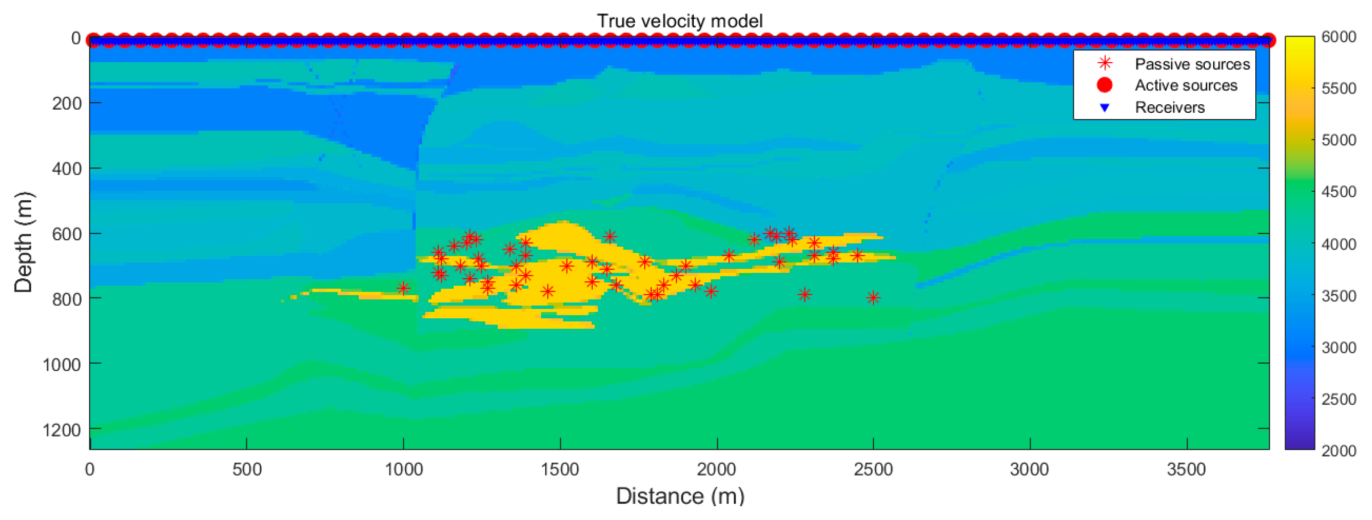
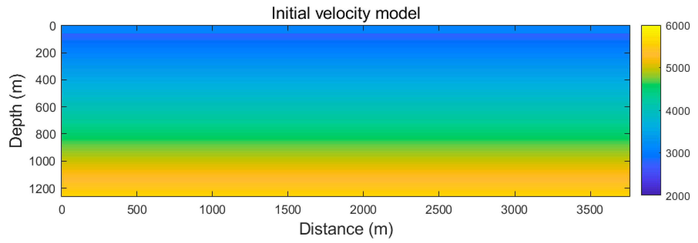
2. Synthetic Datasets

Our goal in generating the synthetic data was to verify the effectiveness of our inversion method. The complexity of the synthetic dataset is not comparable with the field data, so we tried our best to make the synthetic datasets close to the filed datasets. We used a velocity model of a complex metal ore body. The model was modified from a geological ore body model in the Luzong Basin, China and is shown in Figure 1. The deposit consists of several ore bodies. The overall ore body is complexly layered and gently lenticular. Its plane projection is elliptical. The ore body is dome-like in spatial expression, with leached poor iron ore dominating in the center and rich and thick ore surrounding it. Only two of them are relatively large in scale, and the rest are small [34].
We used our own finite-difference program based on the MATLAB software to model both active and passive datasets, which were used for this work. The finite-difference program uses a 8th order accuracy and PML (perfect match layer) boundary condition. The modeling parameters are shown in Table 1. The model size was 376 * 126 with a grid size of 10 m for both dx and dz. There were 376 receivers at the model surface as shown in Figure 1, marked with blue inverted triangles. The distance between each receiver is 10 m. The receiver locations are the same for both active and passive data sets. The active source locations marked with red dots are shown in Figure 1. We use a 20 Hz Ricker wavelet as the source wavelet for the active data set, and 75 shots are generated. The distance between each shot is 50 m. The passive source locations marked with red stars are shown in Figure 1. Fifty passives shots were generated. We assumed that the passive sources had a relative uniform distribution and put the passive source locations around the ore bodies. We generated two passive source datasets. First, we used a 10 Hz source wavelet for all the source locations for one passive source dataset. This dataset was used to test whether the method will work in an ideal case. To make the synthetic test more realistic, another passive dataset used different source wavelets for the other source locations. We also added random noise to different datasets. Six different datasets were generated for future tests, as shown in Table 2.
In order to simulate the lack of low-frequency information in the active source data, we performed high-pass filtering with low cut frequency at 5 Hz on the active source datasets. Figure 2 shows the example shot gathers of the active and passive synthetic seismic datasets. Figure 2a is the active seismic shot gather that was shot at the center of the survey, and Figure 2c is the same shot gather with random noise. Figure 2b is an example passive seismic shot gather with a 10 Hz source wavelet, and Figure 2d is the same shot gather with random noise.

3. Multisource Full Waveform Inversion

3.1. Theory

3.1.1. Conventional Full Waveform Inversion

FWI is used to find a model that generates a synthetic seismic wavefield that fits the real observed seismic wavefield. The conventional FWI workflow is shown in Figure 3. The objective function E can be defined as:
E = i n s j n r u i j d i j 2
where uij is the synthetic seismic data; dij is the observed seismic data; i is the source location; and j is the receiver location. This is a nonlinear inversion problem. FWI usually uses a local optimization algorithm to solve it.

3.1.2. Source Independent Full Waveform Inversion

A successful full waveform inversion needs a good source wavelet estimation of the observed seismic dataset. In real conditions, it is very hard to obtain a good source estimation, especially for the passive seismic dataset. There is one approach called source independent FWI that can solve this problem [32].
We could use Green’s function and source wavelet to replace the uij(m) and dij in Equation (1). The new misfit function is:
E = i n s j n j G i j u S u G i j d S d 2
where G and S are the Green’s function and source wavelet; the * represents the convolution process; and superscripts u and d are the modeled and observed seismic data, respectively. The source independent FWI uses a special misfit function that consists of the convolution of the observed wavefields with a reference trace from the modeled wavefield and the convolution of the modeled wavefields with a reference trace from the observed wavefield. The new misfit function can be written as follows:
E = i n s j n r u i j d i k d i j u i k 2
where uik and dik are the reference traces from the modeled and the observed seismic data at the kth receiver position, respectively. The misfit function E can be rewritten with G and S:
E = i n s j n j G i j u G j k d S u S d G i j d G j k u S u S d 2
The effects of the source wavelets are eliminated as the source wavelet of the observed and the modeled wavefields are equally convolved with both terms in the new misfit function.

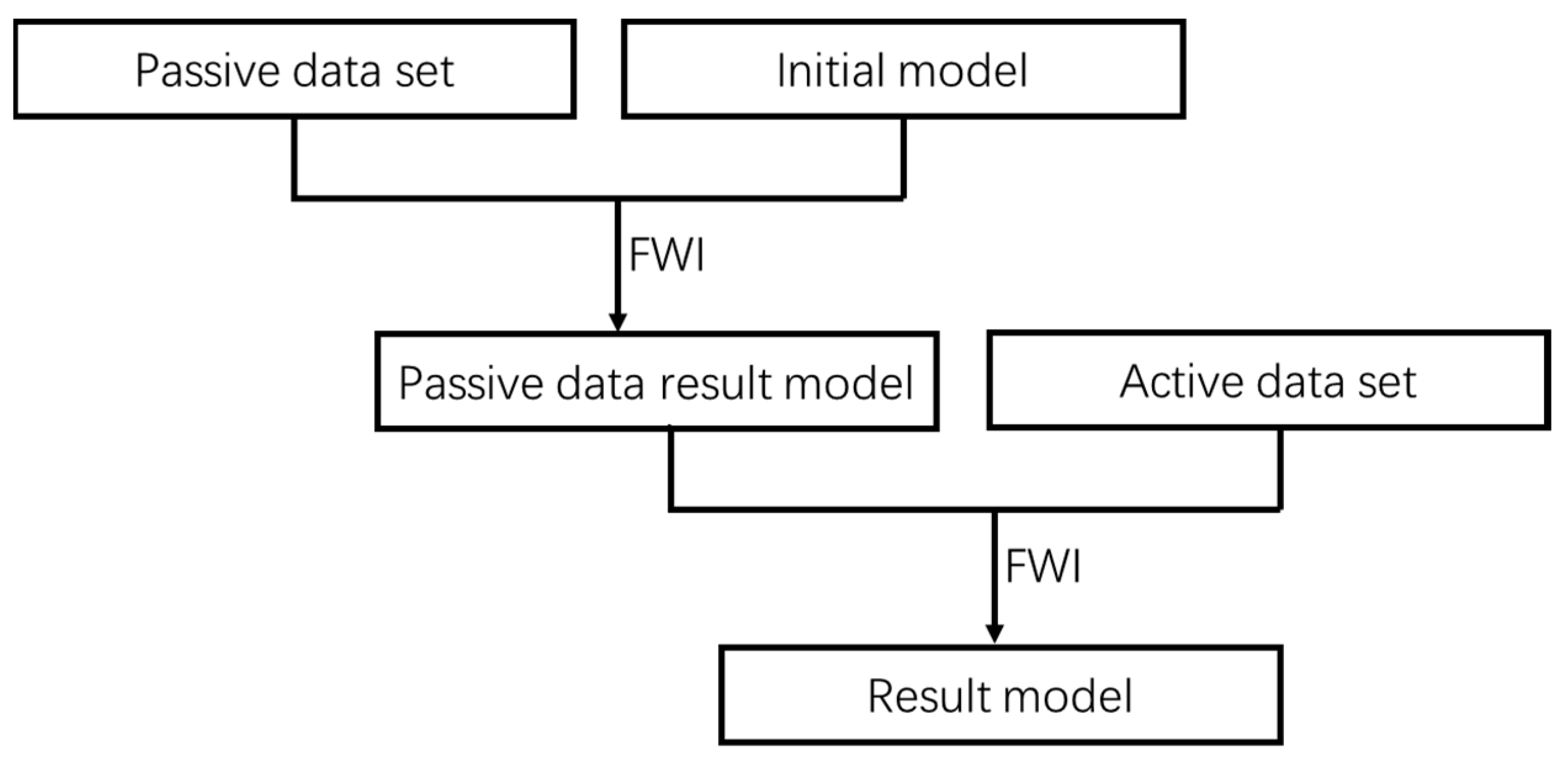
3.1.3. Multisource FWI Workflow

FWI is based on the Born approximation and can be considered as a local optimization problem. The success of active source FWI depends on the good initial model and low-frequency data. However, the real seismic data may not contain good low-frequency information or have a very low signal-to-noise ratio (SNR) in the low-frequency band. The passive seismic data usually carries low-frequency information, and when used to compensate for the active seismic data, it has a more physical basis than pure mathematical methods. Although passive seismic data have the advantages above-mentioned, its weak energy, low signal-to-noise ratio, and unknown source locations and source wavelets also limit its application in FWI.
There are many forms of joint FWI of active source and passive source seismic data. The main idea is to compensate the active source FWI by taking advantage of the richer low-frequency information contained in the passive source data. In general, there are three different approaches.
  • Directly apply FWI to the passive source seismic data to construct an initial model for the active source seismic data FWI;
  • Use the passive seismic data to compensate for the insufficient illumination of the active seismic data [28,30];
  • Merge the active source and passive source seismic data using a specific method to compensate for the low-frequency information; and
  • Use the seismic interferometry method to process the passive source data and generate virtual shot gathers, then directly inverts it to provide an initial model for the active seismic FWI [29].
In this study, we chose the first multisource FWI approach. To further carry out our research, we made the following assumptions. We assumed we could relative correctly locate the passive source locations. This is a strong assumption, but in some cases, we could achieve it. We did not consider the elastic problem. Both forward modeling and inversion were conducted using the acoustic wave equation. The workflow is shown in Figure 4.

3.2. Numerical Examples

To verify our multisource FWI method and workflow, we designed three different numerical tests. We used the same initial velocity model shown in Figure 5 for all tests. First, we tested the method in a near-perfect condition. Second, we tested the condition where we did not know the source wavelet for the active and passive seismic datasets. Finally, we tested how the method works with noise in both the active and passive datasets. We conducted five different tests, as shown in Table 3.

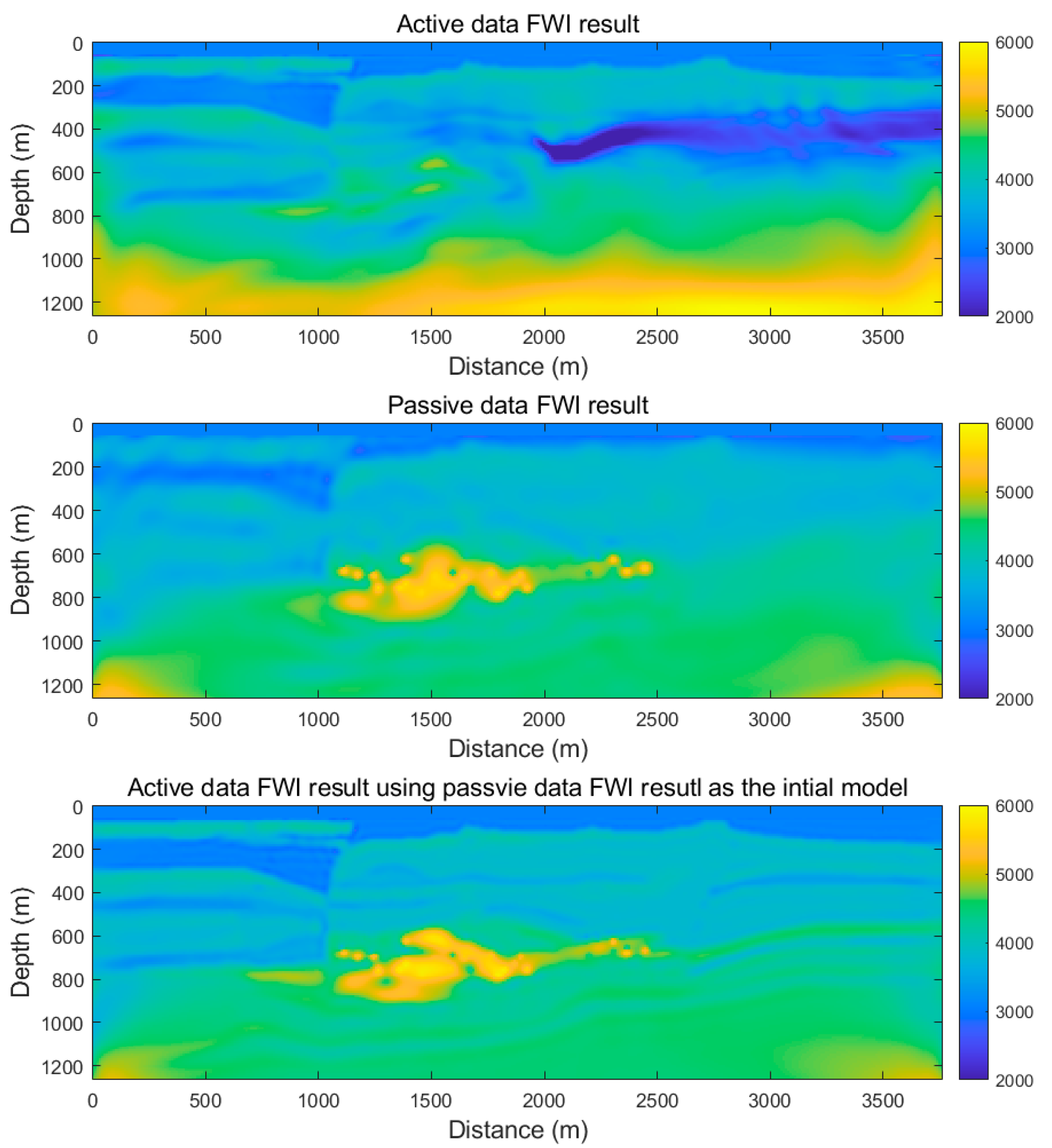
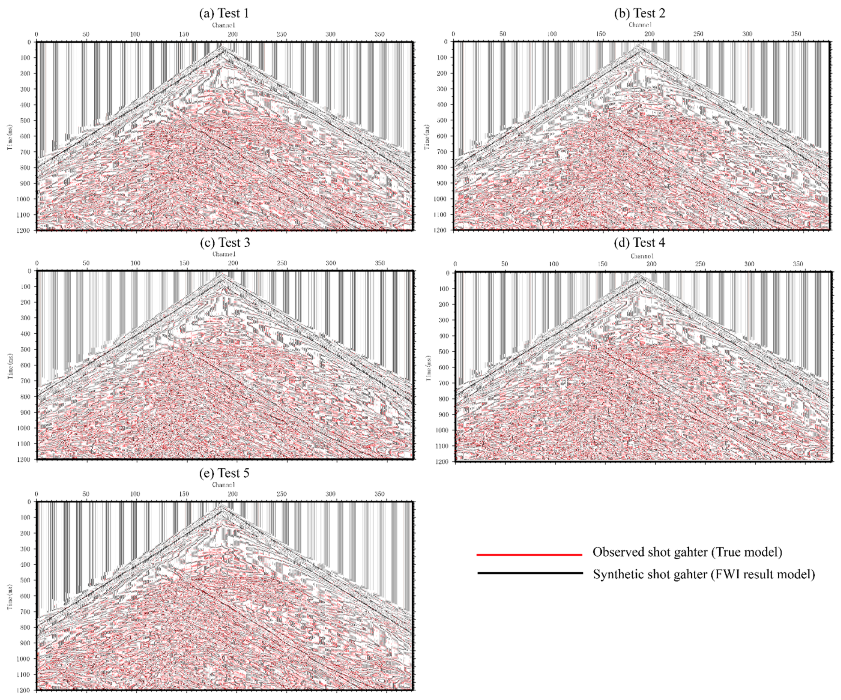
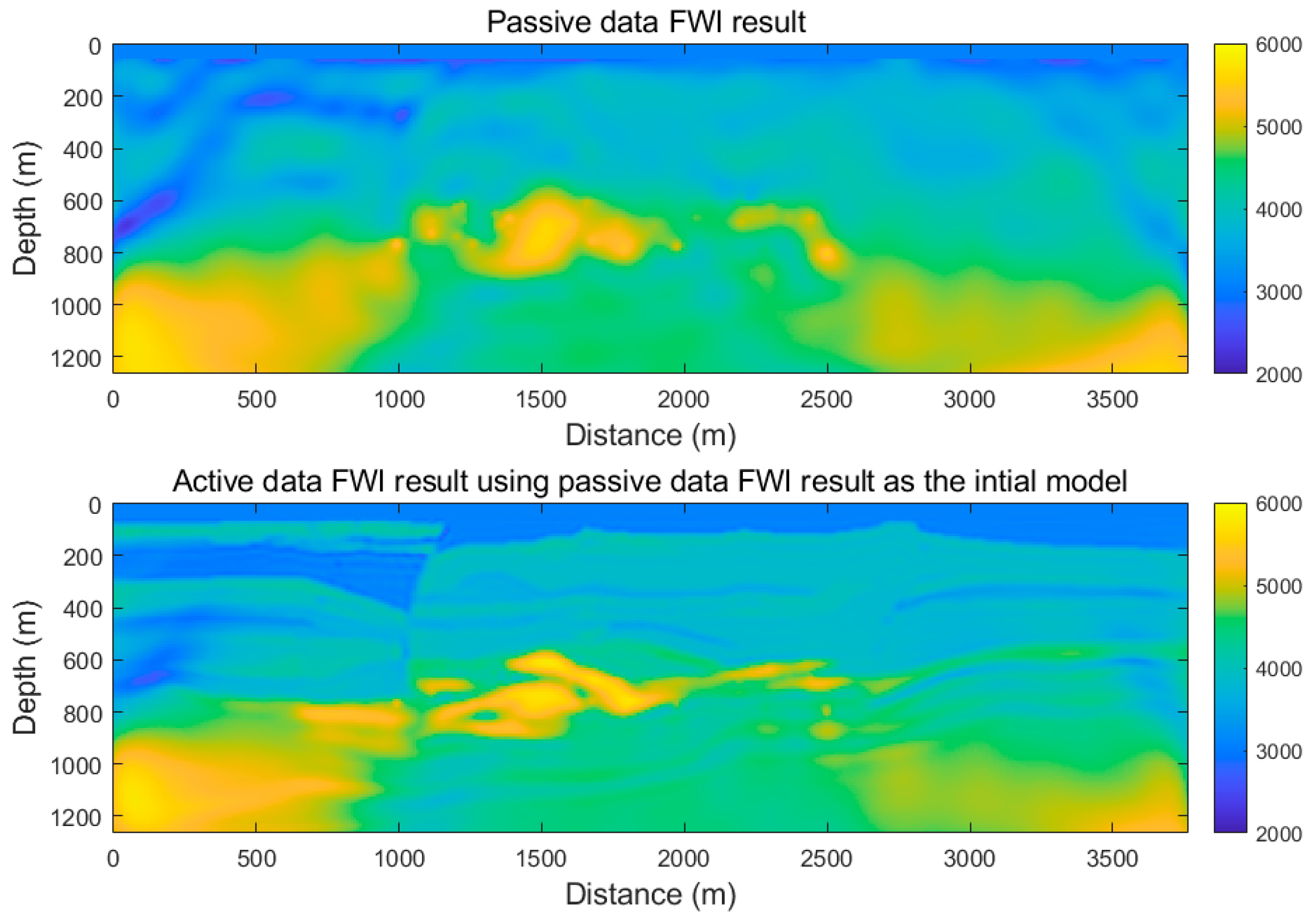
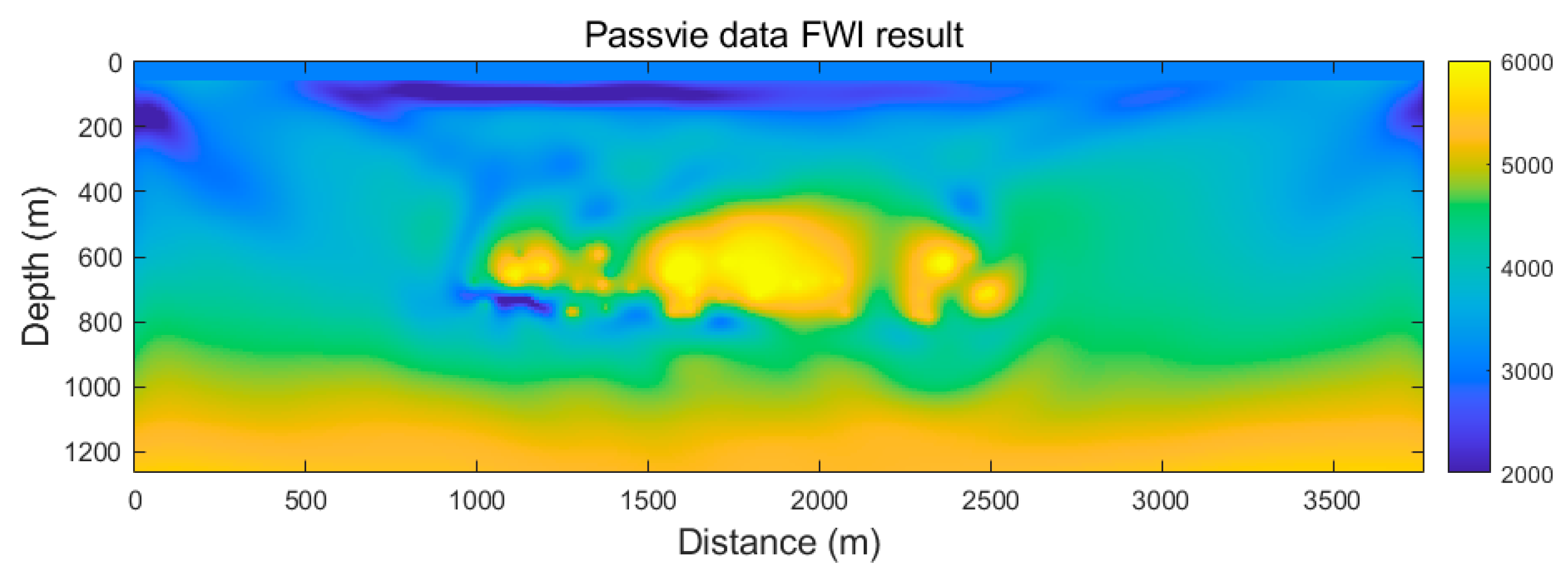
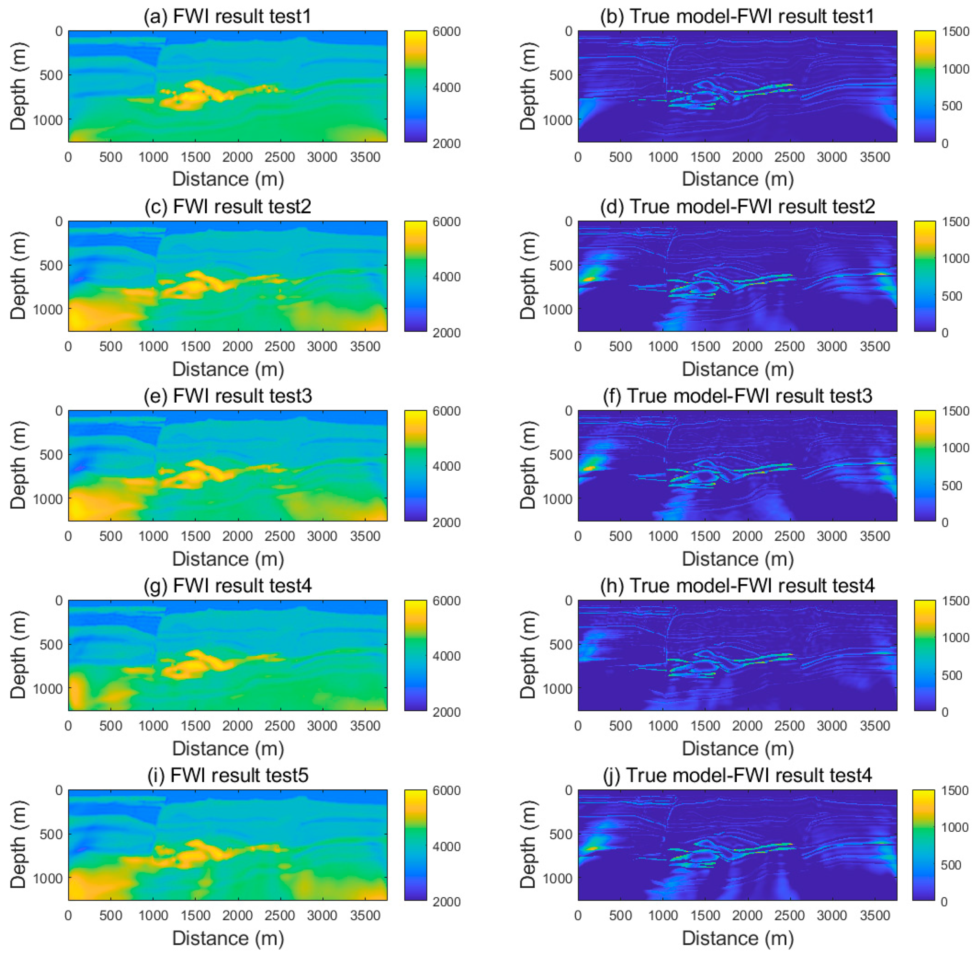
3.2.1. Test 1: Test with Ideal Condition

We conducted a simple numerical test to compare the multisource FWI and conventional active source FWI. We used the synthetic datasets 1 and 3, as shown in Table 2. We assumed that we knew the passive source location and source wavelets for both passive and active sources. First, we applied the multiscale FWI to the active source seismic dataset. The multiscale approach was conducted by filtering the data with different frequency bands (low pass filter with a stop frequency at 24 Hz, 32 Hz, 40 Hz, and 50 Hz). The result of the lower frequency band data was used as the initial model for the higher frequency band data. The upper figure in Figure 6 shows the active source FWI result. Compared with the true velocity model, it provides a relatively correct shallow part of the model. We can roughly see some outlines of the ore body. However, it is difficult to obtain a clear idea of the ore body’s shape. The main reason is that the active source survey is at the surface. The gradients were weak in the deep parts of the model. The insufficient illumination will influence the final results of FWI, and it is hard to invert the deep parts of the model. The lack of low-frequency information of the active seismic dataset also limits the accuracy of the inversion results.
For the multisource FWI, we used the same approach as the active FWI. However, we used the FWI result of the passive source dataset as the initial model for the active source dataset. The middle figure in Figure 6 shows the FWI result of the passive source dataset. Although the resolution of the shallow layer was not as good as the result of the active source dataset, it provided a much better result of the ore body. This is because the passive sources are located around the ore body, which has a better illumination condition. The rich information of the low-frequency information of the passive dataset also improves the stability and accuracy of the inversion. The lower figure of Figure 6 shows the FWI results of the active source dataset using the passive source dataset that was the result of the initial model. The result velocity model was significantly improved by using both passive and active source data. We could see the details of both the shallow and deep parts of the model. The shapes of the two relatively large-scale and even some small ore bodies are clearly imaged.

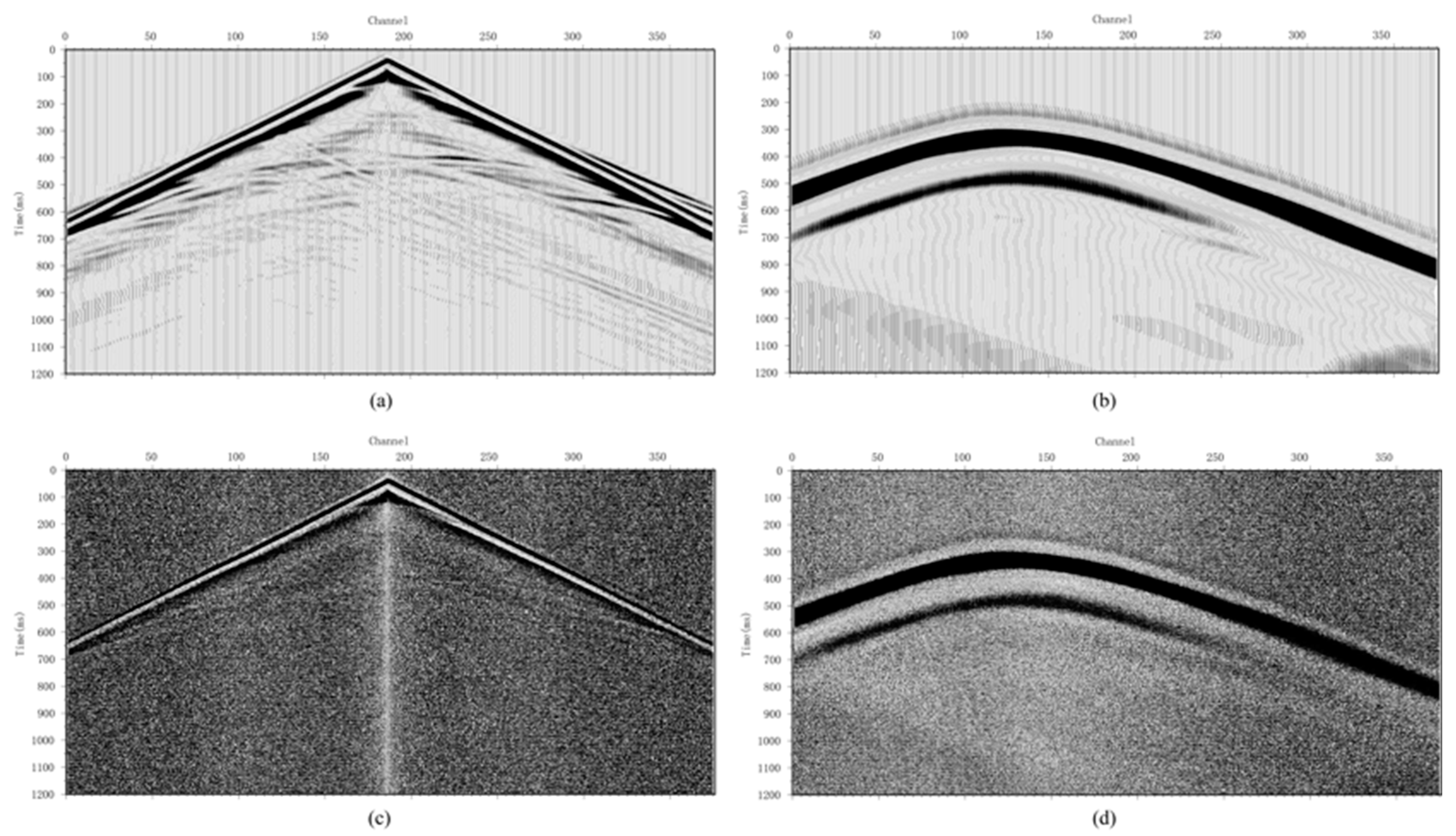
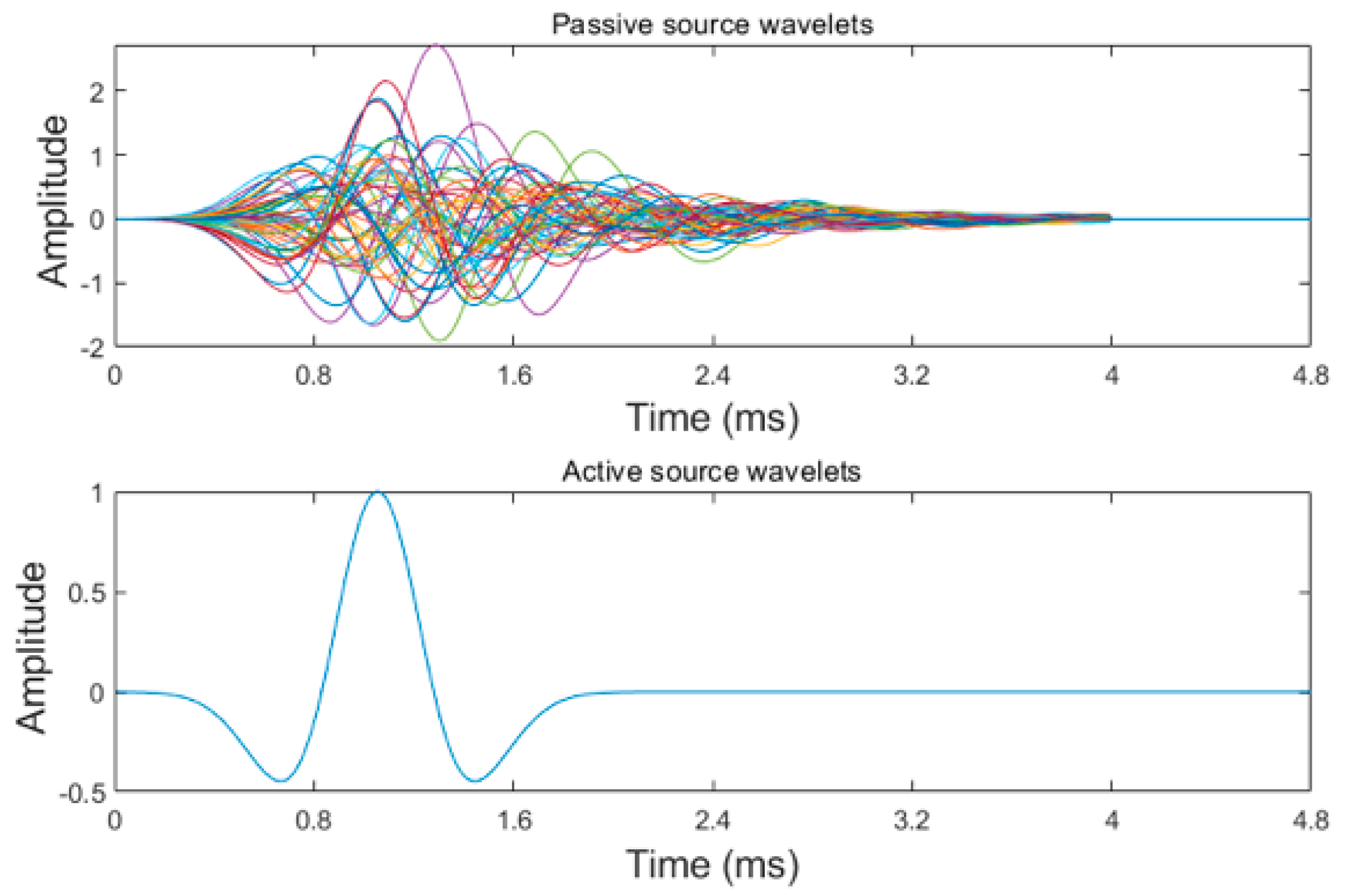
3.2.2. Test 2: Numerical Test with Unknown Source Wavelets

The previous simple test showed that our multisource FWI approach works in an ideal condition. In this test, we weakened the preconditions for our method. In a real case, the inaccuracy of the source location and wavelets will also affect the inversion result. The source wavelets are more difficult to obtain compared with source locations. We simulated the condition that we did not know the source wavelets for the passive and active datasets. We used the synthetic datasets 1 and 4 as shown in Table 2. Figure 7 shows the source wavelets used to generate the synthetic datasets. The passive source wavelets at different source locations were generated by using a 10 Hz Ricker wavelet convoluted with a random sequence. We used the source independent FWI algorithm that did not rely on the source wavelet, which can overcome the influence of the inaccuracy of the passive source wavelets on the inversion result. The low-frequency information of the passive source data can be used to obtain the large-scale structure information of the model. The resulting model of the passive source data can be used as the initial model for the FWI of the active source data that is missing low-frequency information. For the active source data FWI, we used the same multiscale approach as in the previous test.
Figure 8 shows the source independent multisource FWI inversion result. The upper figure is the source independent passive source FWI result. It provided relatively correct large-scale information of the model. The result was worse than the passive FWI result shown in Figure 6. This is because both the passive datasets and FWI approach were different. The lower figure of Figure 8 shows the source independent active FWI result using the passive source FWI result as the initial model. The result shows that we could obtain a similarly good result even when we did not know the correct source wavelets.

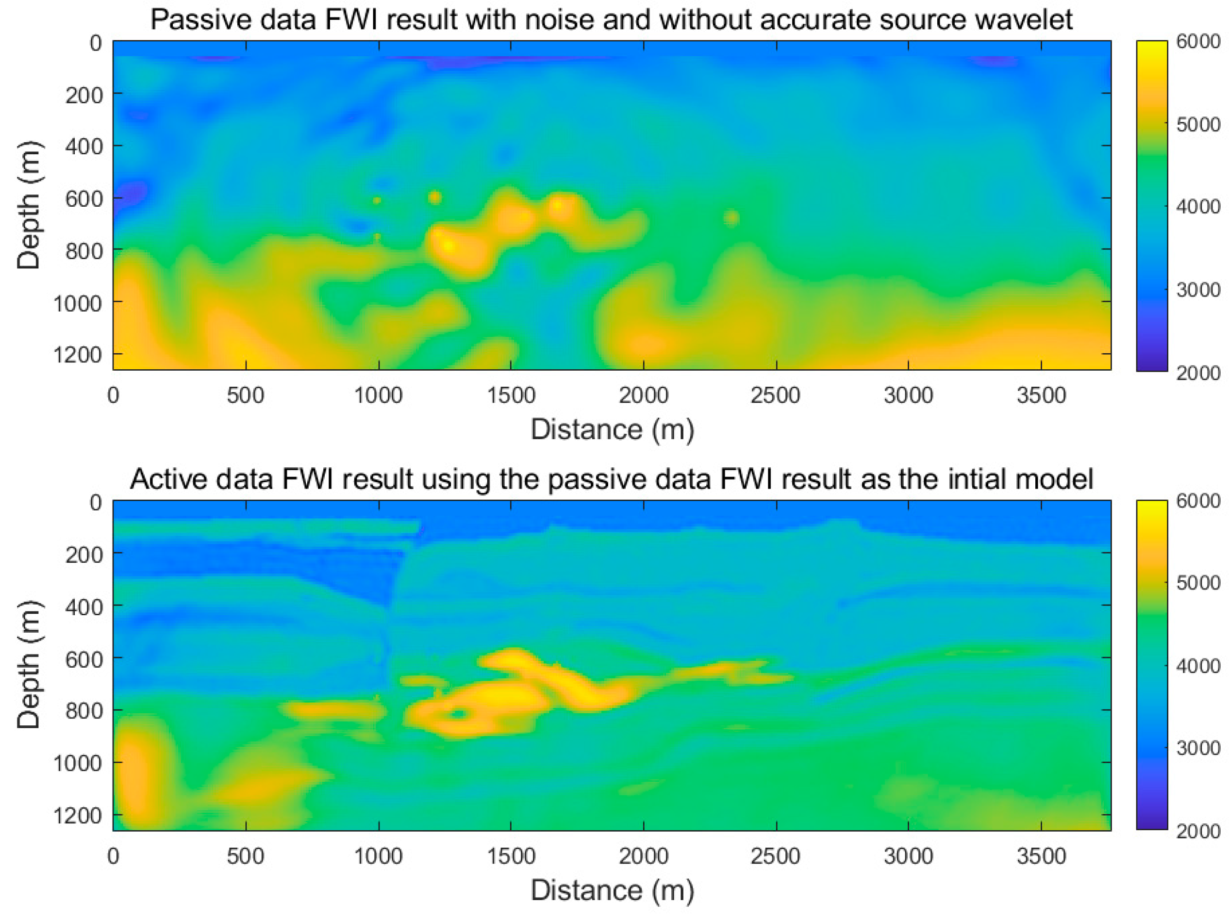
3.2.3. Test 3: Numerical Test with Noise and Unknown Source Wavelets

We also added noise to the passive and active source datasets to test the multisource FWI in a more realistic condition. We used synthetic datasets 2 and 5, as shown in Table 2, in this test. A relatively strong noise (30 db Gaussian white noise) was added to both the active and passive source seismic datasets. We chose this noise level because most of the real datasets could reach this level after processing. Figure 9 shows the conventional FWI result of the noisy passive source seismic dataset. The inversion failed to converge due to the noise and unknown source wavelets when using the conventional FWI approach. Then, we tried the source independent FWI approach that was the same as test 2. Figure 10 shows the source independent FWI results of the noise datasets. The result is very similar to the FWI result in test 1, which is shown in Figure 6. This means that the source independent FWI method can handle the noise dataset quite well. However, due to the influence of noise, the final inversion results were slightly worse than test 1.

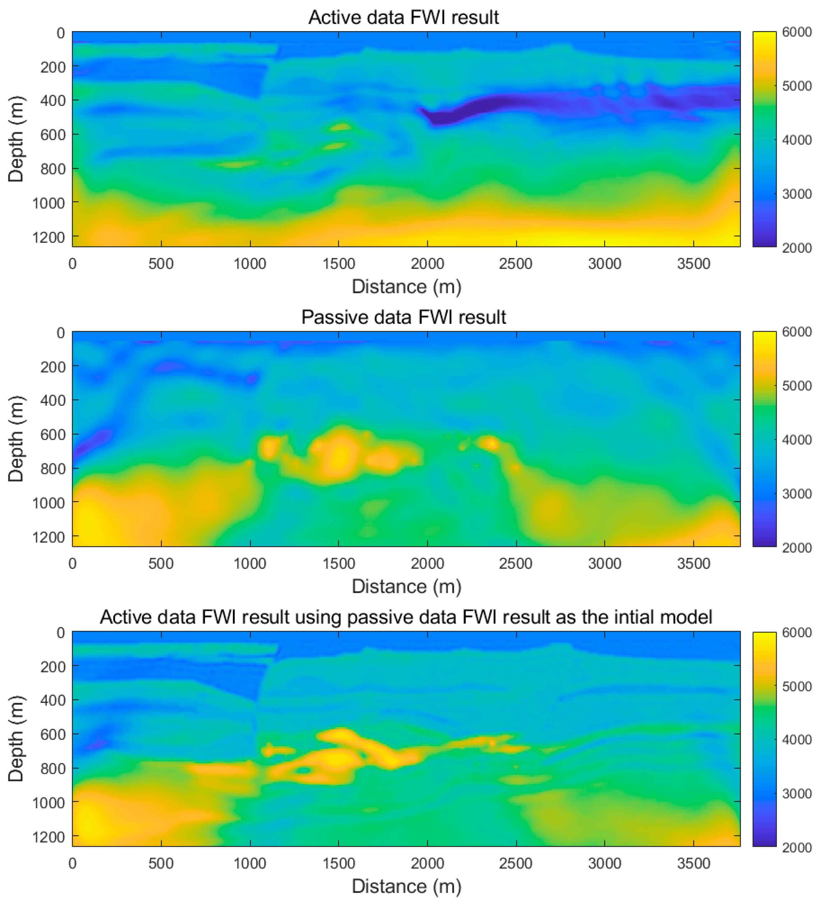
3.2.4. Test 4: Numerical Test with Noise, Unknown Source Wavelets, and Less Passive Shots

In a real case, we may not get 50 usable passive sources records as we did here. We also tested the condition where we were only able to obtain 10 passive source records. We randomly picked 10 passive shots from dataset 5. We applied the same inversion procedure to datasets 2 and 6. First, we applied source independent FWI to dataset 6. Then, we used the inversion result as the initial model for dataset 2. Figure 11 shows the inversion results. From the results, we could see that even if we only used 10 passive shots, the passive dataset inversion still builds up large-scale information of the velocity structure. This provides a useful initial model for the active dataset inversion. The active dataset inversion result was comparable with the previous one.

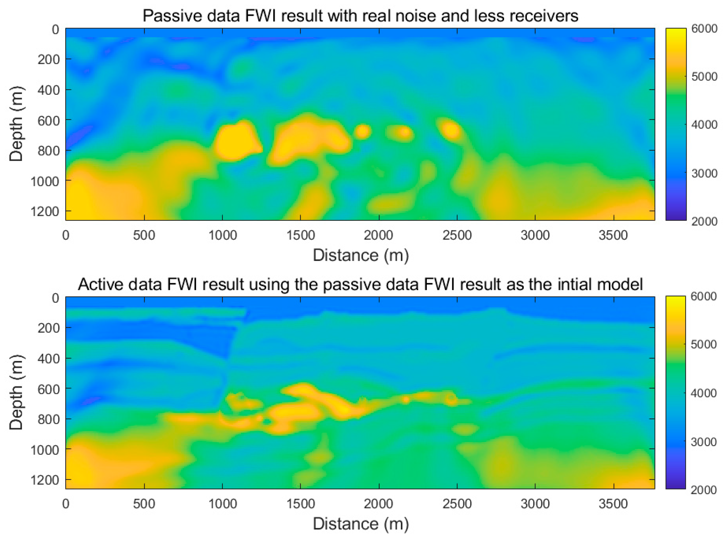
3.2.5. Test 5: Numerical Test with Real Noise, Unknown Source Wavelets and Fewer Passive Shots and Fewer Receivers for Both Passive and Active Dataset

In addition, we also tested our method with real noise data and less dense acquisition geometry. We took the real background noise from a mining area. The noise was directly added to the synthetic datasets. We also used only 10 randomly picked passive shots (dataset 7). We took every 5th receiver channel from both passive and active datasets to simulate the less dense acquisition. Figure 12 shows the example shot gathers with real noise and less dense acquisition geometry. The same inversion perdure was applied to datasets 7 and 8. First, we applied source independent FWI to dataset 7. Then, we used the inversion result as the initial model for dataset 8. Figure 13 shows the inversion results. The results show that the method works fine in real noise conditions and sparse acquisition geometry.

4. Discussion

Figure 14 shows the final FWI result and the differences between the final FWI test and the true model for each test. The ideal test gave the best result. We can clearly identify the geometry of the main ore bodies. However, the velocity of the ore body obtained by the FWI was about 10% lower than the actual velocity. Figure 15 shows the comparison between the observed active shot gather (generated from the true model) and the synthetic active shot gather (generated from each multisource FWI test). We found that the data fitting was pretty good for all the tests. When adding different noise and making the data set sparse, we could still obtain a reasonable result using our multisource FWI approach.
There are also some limitations to our current numerical tests. We chose a complex model built from a real mining area, added real noise to the synthetic datasets, and used sparse acquisition geometry. The synthetic datasets were still idealized compared with real datasets. We may also face many other issues in the real datasets such as complex noise characteristics, discontinuity, and complexity of the shot gather signal and elastic effects. However, these were not within our study scope. It is possible to minimize these effects by preprocessing the dataset in some real cases.
Another main assumption was that the location of the seismic sources is known. Numerical tests 4 and 5 showed that we could only use a few passive shots to build a suitable initial model for the active data inversion. We believe that it is possible to obtain a few usable passive shots in some actual cases.
The best way to test our multisource FWI approach is to apply it to an actual dataset. However, there is no suitable real dataset available for testing at present, which can be considered as research content in the future.

5. Conclusions

The active seismic data acquired in the metal mine area usually lacks low-frequency information. It is challenging to use only active source data to obtain good imaging of the ore bodies. The multisource FWI method uses effective low-frequency signals from the original passive source information, proving the potential use of low-frequency passive source information in constructing large-scale velocity models. The passive seismic FWI can provide a good initial model for the active seismic FWI, thus reducing the dependence of the active seismic FWI on the initial model and low-frequency information. We chose a complex velocity model from a mining area and generated serval datasets to test our method. The numerical results of the perfect condition show that the multisource seismic full waveform inversion could obtain a suitable result for high-resolution seismic imaging of metal ore bodies. The method also worked fine when the source wavelets are unknown, and the datasets had a relatively high noise level by introducing the source independent approach.

Author Contributions

Conceptualization, F.Z. and P.Z.; Methodology, F.Z. and P.Z.; Software, P.Z.; Validation, F.Z., P.Z., Z.X., X.G. and L.H.; Formal analysis, F.Z., P.Z. and Z.X.; Investigation, P.Z. and X.G.; Resources, F.Z. and Z.X.; Data curation, P.Z.; Writing—original draft preparation, F.Z. and P.Z.; Writing—review and editing, Z.X., X.G. and L.H.; Visualization, F.Z.; Supervision and project administration: F.Z. and P.Z. All authors have read and agreed to the published version of the manuscript.

Funding

This research was funded by the National Natural Science Foundation of China (No. 41974138, 42004106, 42074151, 41874139, 42130805, and 42074154), the Natural Science Foundation of Jilin Province (No. YDZJ202101ZYTS020), the National Key R&D Program of China (2020YFE0201300), and the Lift Project for Young Science and Technology Talents of Jilin Province (No. QT202116).

Data Availability Statement

The data presented in this study are available on request from the corresponding author.

Acknowledgments

We thank numerous people from Jilin University for their suggestions about this work. We used MATLAB and GMT for modeling, processing, and visualization.

Conflicts of Interest

The authors declare no conflict of interest. The funders had no role in the design of the study, in the collection, analyses, or interpretation of data, in the writing of the manuscript, or in the decision to publish the results.

References

  1. Malehmir, A.; Dahlin, P.; Lundberg, E.; Juhlin, C.; Sjöström, H.; Högdahl, K. Reflection seismic investigations in the Dannemora area, central Sweden: Insights into the geometry of polyphase deformation zones and magnetite-skarn deposits. J. Geophys. Res. Solid Earth 2011, 116, B11307. [Google Scholar] [CrossRef]
  2. Malehmir, A.; Durrheim, R.; Bellefleur, G.; Urosevic, M.; Juhlin, C.; White, D.J.; Milkereit, B.; Campbell, G. Seismic methods in mineral exploration and mine planning: A general overview of past and present case histories and a look into the future. Geophysics 2012, 77, WC173–WC190. [Google Scholar] [CrossRef] [Green Version]
  3. Place, J.; Malehmir, A.; Högdahl, K.; Juhlin, C.; Nilsson, K.P. Seismic characterization of the Grangesberg iron deposit and its mining-induced structures, central Sweden. Interpret. J. Subsurf. Charact. 2015, 3, Sy41–Sy56. [Google Scholar] [CrossRef]
  4. Singh, B.; Malinowski, M.; Hloušek, F.; Koivisto, E.; Heinonen, S.; Hellwig, O.; Buske, S.; Chamarczuk, M.; Juurela, S. Sparse 3D Seismic Imaging in the Kylylahti Mine Area, Eastern Finland: Comparison of Time Versus Depth Approach. Minerals 2019, 9, 305. [Google Scholar] [CrossRef] [Green Version]
  5. Bräunig, L.; Buske, S.; Malehmir, A.; Bäckström, E.; Schön, M.; Marsden, P. Seismic depth imaging of iron-oxide deposits and their host rocks in the Ludvika mining area of central Sweden. Geophys. Prospect. 2020, 68, 24–43. [Google Scholar] [CrossRef] [Green Version]
  6. Lailly, P.; Bednar, J. The seismic inverse problem as a sequence of before stack migrations. In Proceedings of the Conference on Inverse Scattering—Theory and Application, Tulsa, OK, USA, 16–18 May 1983. [Google Scholar]
  7. Tarantola, A. Inversion of seismic reflection data in the acoustic approximation. Geophysics 1984, 49, 1259–1266. [Google Scholar] [CrossRef]
  8. Pratt, R.G. Seismic waveform inversion in the frequency domain, Part 1: Theory and verification in a physical scale model. Geophysics 1999, 64, 888–901. [Google Scholar] [CrossRef] [Green Version]
  9. Pratt, R.G.; Shipp, R.M. Seismic waveform inversion in the frequency domain, Part 2: Fault delineation in sediments using crosshole data. Geophysics 1999, 64, 902–914. [Google Scholar] [CrossRef]
  10. Sirgue, L.; Pratt, R.G. Efficient waveform inversion and imaging: A strategy for selecting temporal frequencies. Geophysics 2004, 69, 231–248. [Google Scholar] [CrossRef] [Green Version]
  11. Brenders, A.J.; Pratt, R.G. Full waveform tomography for lithospheric imaging: Results from a blind test in a realistic crustal model. Geophys. J. Int. 2007, 168, 133–151. [Google Scholar] [CrossRef] [Green Version]
  12. Brossier, R.; Operto, S.; Virieux, J. Seismic imaging of complex onshore structures by 2D elastic frequency-domain full-waveform inversion. Geophysics 2009, 74, WCC105–WCC118. [Google Scholar] [CrossRef]
  13. Virieux, J.; Operto, S. An overview of full-waveform inversion in exploration geophysics. Geophysics 2009, 74, WCC1–WCC26. [Google Scholar] [CrossRef]
  14. Kamei, R.; Pratt, R.G.; Tsuji, T. Waveform tomography imaging of a megasplay fault system in the seismogenic Nankai subduction zone. Earth Planet. Sci. Lett. 2012, 317, 343–353. [Google Scholar] [CrossRef]
  15. Warner, M.; Ratcliffe, A.; Nangoo, T.; Morgan, J.; Umpleby, A.; Shah, N.; Vinje, V.; Štekl, I.; Guasch, L.; Win, C.; et al. Anisotropic 3D full-waveform inversion. Geophysics 2013, 78, R59–R80. [Google Scholar] [CrossRef]
  16. Yao, G.; Wu, D.; Wang, S.-X. A review on reflection-waveform inversion. Pet. Sci. 2020, 17, 334–351. [Google Scholar] [CrossRef] [Green Version]
  17. Sun, H.-Y.; Han, L.-G.; Han, M.; Wang, Z.-Q. Elastic full waveform inversion based on visibility analysis and energy compensation for metallic deposit exploration. Chin. J. Geophys. 2015, 58, 4605–4616. [Google Scholar]
  18. Egorov, A.; Bóna, A.; Pevzner, R.; Tertyshnikov, K. Potential of full waveform inversion of vertical hard rock environment seismic profile data in. ASEG Ext. Abstr. 2019, 2018, 1–3. [Google Scholar] [CrossRef] [Green Version]
  19. Mao, B.; Han, L.; Hu, Y.; Zhang, P. Low-frequency seismic data reconstruction based similarity phenomenon for metal mine full waveform inversion in frequency domain. Chin. J. Geophys. 2019, 62, 4010–4019. [Google Scholar]
  20. Hlousek, F.; Malinowski, M.; Buske, S.; Bräunig, L.; Singh, B.; Malehmir, A.; Markovic, M.; Koivisto, E.; Heinonen, S.; Sito, L.; et al. A tailored workflow for advanced high-resolution seismic imaging of mineral exploration targets. In Mineral Exploration Symposium; European Association of Geoscientists & Engineers: Houten, The Netherlands, 2020; pp. 1–3. [Google Scholar]
  21. Singh, B.; Górszczyk, A.; Malehmir, A.; Hlousek, F.; Buske, S.; Sito, L.; Marsden, P. 3D Velocity Model Building in Hardrock Environment Using FWI: A Case Study from Blötberget Mine, Sweden. In Proceedings of the NSG2020 3rd Conference on Geophysics for Mineral Exploration and Mining, Belgrade, Srbija, 30 August–3 September 2020; pp. 1–5. [Google Scholar]
  22. Song, C.; Wu, Z.; Alkhalifah, T. Passive seismic event estimation using multiscattering waveform inversion. Geophysics 2019, 84, KS59–KS69. [Google Scholar] [CrossRef]
  23. Lyu, B.; Nakata, N. Iterative passive-source location estimation and velocity inversion using geometric-mean reverse-time migration and full-waveform inversion. Geophys. J. Int. 2020, 223, 1935–1947. [Google Scholar] [CrossRef]
  24. Wang, H.; Guo, Q.; Alkhalifah, T.; Wu, Z. Regularized elastic passive equivalent source inversion with full-waveform inversion: Application to a field monitoring microseismic data set. Geophysics 2020, 85, Ks207–Ks219. [Google Scholar] [CrossRef]
  25. Kamei, R.; Lumley, D. Passive seismic imaging and velocity inversion using full wavefield methods. In SEG Technical Program Expanded Abstracts 2014; Society of Exploration Geophysicists: Denver, CO, USA, 2014; pp. 2273–2277. [Google Scholar]
  26. Kamei, R.; Lumley, D. Full waveform inversion of repeating seismic events to estimate time-lapse velocity changes. Geophys. J. Int. 2017, 209, 1239–1264. [Google Scholar] [CrossRef]
  27. Sun, J.; Xue, Z.; Zhu, T.; Fomel, S.; Nakata, N. Full-waveform inversion of passive seismic data for sources and velocities. In SEG Technical Program Expanded Abstracts 2016; Society of Exploration Geophysicists: Dallas, TX, USA, 2016; pp. 1405–1410. [Google Scholar]
  28. Zhang, P.; Han, L.G.; Jin, Z.Y.; Zhang, F.J. Passive Source Illumination Compensation Based Full Waveform Inversion. In Proceedings of the 78th EAGE Conference and Exhibition 2016, online, 30 May–2 June 2016; pp. 1–3. [Google Scholar]
  29. Zhang, P.; Han, L.; Yin, Y.; Feng, Q. Passive seismic full waveform inversion using reconstructed body-waves for subsurface velocity construction. Explor. Geophys. 2019, 50, 124–135. [Google Scholar] [CrossRef]
  30. Zhang, P.; Xing, Z.Z.; Hu, Y. Velocity construction using active and passive multi-component seismic data based on elastic full waveform inversion. Chin. J. Geophys. 2019, 62, 3974–3987. [Google Scholar]
  31. Choi, Y.; Shin, C.; Min, D.J.; Ha, T. Efficient calculation of the steepest descent direction for source-independent seismic waveform inversion: An amplitude approach. J. Comput. Phys. 2005, 208, 455–468. [Google Scholar] [CrossRef]
  32. Choi, Y.; Alkhalifah, T. Source-independent time-domain waveform inversion using convolved wavefields: Application to the encoded multisource waveform inversion. Geophysics 2011, 76, R125–R134. [Google Scholar] [CrossRef] [Green Version]
  33. Zhang, P.; Wu, R.-S.; Han, L. Source-independent seismic envelope inversion based on the direct envelope Fréchet derivative. Geophysics 2018, 83, R581–R595. [Google Scholar] [CrossRef]
  34. Lian, Y.; Lv, Q.; Han, L.; Zhao, J. The Research of Seismic Modeling in Complex Metal Ore Region-Take Luzong Luohe-Nihe-Dabaozhuang Deposits for an Example. Acta Geol. Sin. 2011, 85, 887–899. [Google Scholar]
Figure 1. The complex velocity model of a metal ore body from the Luzong Basin, China. The active sources, passives sources, and receiver locations are marked with different marks, as shown in the right upper corner of the figure.
Minerals 12 00004 g001
Figure 2. Example of shot gathers of the active and passive synthetic seismic datasets used in this work. (a) An example of the active shot gather. (b) An example of the passive shot gather. (c) An example of the active shot gather with noise. (d) An example of a passive shot gather with noise.
Minerals 12 00004 g002
Figure 3. The conventional FWI workflow.
Minerals 12 00004 g003
Figure 4. Multisource FWI workflow.
Minerals 12 00004 g004
Figure 5. The initial velocity model for FWI.
Minerals 12 00004 g005
Figure 6. The results of numerical test one. The upper figure shows the FWI result only using the active dataset (dataset 1 in Table 2). The middle figure shows that the FWI result only uses the passive dataset (dataset 3 in Table 2). The lower figure shows the FWI result when using both active and passive datasets.
Minerals 12 00004 g006
Figure 7. The true source wavelets for the passive datasets and the different color lines means different source wavelets (upper figure), and active dataset (lower figure).
Minerals 12 00004 g007
Figure 8. The source independent multisource FWI results. The upper figure is the passive source FWI results and the lower figure is the active source FWI result using the passive source FWI result as the initial model.
Minerals 12 00004 g008
Figure 9. The conventional FWI result of the passive source data with noise.
Minerals 12 00004 g009
Figure 10. The source independent multisource FWI results of the noise datasets. The upper figure shows that the FWI result only uses the active dataset. The middle figure shows the FWI result only uses the passive dataset. The lower figure shows the FWI result when using both the active and passive dataset.
Minerals 12 00004 g010
Figure 11. The source independent multisource FWI results of the noise datasets with less passive shots. The upper figure shows the FWI result only using the passive dataset. The lower figure shows the FWI result when using both active and passive datasets.
Minerals 12 00004 g011
Figure 12. Example shot gathers of the active (right) and passive (left) synthetic seismic datasets with real noise.
Minerals 12 00004 g012
Figure 13. The source independent multisource FWI results of the real noise datasets with less passive shots and less receivers. The upper figure shows the FWI result only using the passive dataset. The lower figure shows the FWI result when using both active and passive datasets.
Minerals 12 00004 g013
Figure 14. The comparison of the different multisource FWI tests. (a,c,e,g,i) are the final FWI results for tests 1–5; (b,d,f,h,j) are the differences between the final FWI results and the true model for tests 1–5.
Minerals 12 00004 g014
Figure 15. The comparison between the observed shot gather and synthetic shot gather from the different multisource FWI tests. The synthetic shot gather (black) is plotted on top of the observed shot gather (red); (ae) are the comparison for tests 1–5.
Minerals 12 00004 g015
Table 1. Modeling parameters for the active and passive seismic datasets.
Parameters/Data SetsThe Active Seismic DatasetThe Passive Seismic Dataset
Source wavelet20 Hz Ricker wavelet10 Hz Ricker wavelet, or 10 Hz Ricker wavelet convoluted with random sequences
Model size (nx × nz)376 × 126376 × 126
Model dx and dz10 m10 m
Sample rate/Record length0.8 ms/2 s0.8 ms/2 s
Source number7550
Receiver number376376
Table 2. The active and passive seismic datasets were generated for the tests.
Datasets
1. Dataset 1: Active dataset without low frequencies information (no data below 5 Hz);
2. Dataset 2: Dataset 1 with random noise;
3. Dataset 3: Passive dataset with 10 Hz source wavelet for all the source locations;
4. Dataset 4: Passive dataset with different source wavelets for different source locations;
5. Dataset 5: Dataset 4 with random noise;
6. Dataset 6: Ten randomly picked passive shot gathers from dataset 5;
7. Dataset 7: Ten randomly picked pass shot gathers from dataset 4 with real noise, and every 5th receiver channel is used;
8. Dataset 8: Dataset 1 with real noise and every 5th receiver channel is used.
Table 3. Numerical tests for the multisource FWI method.
Tests
1. Test 1 (noise-free, known source locations and known one single wavelet for all source locations, use datasets 1 and 3, the conventional FWI)
2. Test 2 (noise-free, known source locations and unknown wavelets for each source location, use datasets 1 and 4, the source-independent FWI)
3. Test 3 (with noise, known source locations and unknown wavelets for each source location, use datasets 2 and 5, the source-independent FWI)
4. Test 4 (fewer passive data, with noise, known source locations and unknown wavelets for each source location, use datasets 2 and 6, the source-independent FWI)
5. Test 5 (fewer passive data, with noise, known source locations and unknown wavelets for each source location, fewer receivers for both active and passive data, use datasets 7 and 8, the source-independent FWI)
Publisher’s Note: MDPI stays neutral with regard to jurisdictional claims in published maps and institutional affiliations.

