Testing Five Nonlinear Equations for Quantifying Leaf Area Inequality of Semiarundinaria densiflora

Abstract

Accurately quantifying the inequality of plant organ size distributions, such as leaf area, is essential for understanding plant resource allocation strategies, and this is commonly achieved using Lorenz curves. Previous studies have shown that the performance equation (PE) and its generalized form (GPE) effectively describe Lorenz curves that are rotated 135° counterclockwise around the origin and shifted rightward by $\sqrt{2}$ units. However, few studies have compared the fitting performance of PE (and GPE) with other traditional equations generating Lorenz curves in modeling empirical leaf area distributions, and even fewer have considered the validity of linear approximation assumptions in these nonlinear models. To address this gap, we quantified the inequality of leaf area distributions in Semiarundinaria densiflora, a bamboo species for which the abundant and measurable leaves per culm provide an ideal system for examining the ecological strategies underlying leaf allocation patterns. Five nonlinear models were employed to fit the leaf area distribution: PE, GPE, the Sarabia equation (SarabiaE), the Sarabia–Castillo–Slottje equation (SCSE), and the Sitthiyot–Holasut equation (SHE). Model performance was assessed using root-mean-square error (RMSE) and Akaike information criterion (AIC), while nonlinearity curvature measures were applied to evaluate the close-to-linear behavior of parameter estimates. In addition, the Lorenz asymmetry coefficient (LAC) was used to quantify the asymmetry of the Lorenz curves. Our results showed a clear trade-off between predictive accuracy and linear approximation behavior. Among the five models, GPE achieved the best fit, with the lowest RMSE and AIC values, yet did not show good close-to-linear behavior. In contrast, SHE provided the poorest fit but demonstrated the strongest close-to-linear properties. LAC values indicated that relatively abundant, larger leaves disproportionately contributed to the inequality in leaf area distribution. These findings highlight an inherent trade-off in using Lorenz-based models to describe leaf area frequency distributions: predictive accuracy does not necessarily align with statistical validity. By integrating model fit, nonlinearity diagnostics, and asymmetry assessment, this study provides new perspectives and methodological tools for future investigations into inequality in plant organ size distributions and their ecological significance.

1. Introduction

Leaves play a central role in plant growth and development by capturing light energy, regulating gas exchange, and influencing water and nutrient dynamics [1,2,3,4]. Among the many traits that characterize leaves, leaf area is one of the most important functional attributes, as it directly determines the photosynthetic capacity of individual plants and contributes to their competitive performance within ecological communities [5,6,7]. Because variation in leaf area underlies differences in resource acquisition and carbon balance [8,9,10], an accurate quantification of the frequency distribution of leaf area is essential for understanding plant physiology, population structure, and ecological interactions. Capturing not only mean values but also the inequality of leaf area distributions can therefore provide deeper insights into how plants allocate resources and adapt to their environments.

In economics, the Gini coefficient is widely used to measure the inequality of household incomes [11,12]. It is derived from the Lorenz curve, which describes the relationship between the cumulative proportion of household income and the cumulative proportion of the number of households [13,14]. Under conditions of perfect equality, the Lorenz curve coincides with the 1:1 line (i.e., y = x), and the Gini coefficient quantifies the extent to which the Lorenz curve deviates from this line of absolute equality. Specifically, it is defined as the ratio of the area between the Lorenz curve and the line of equality to the total area of the right isosceles triangle beneath the line of absolute equality. Thus, the Gini coefficient ranges between 0 and 1, with values closer to 0 indicating greater equality and values closer to 1 indicating stronger inequality.

The Gini coefficient has proven to be a valuable tool for quantifying inequality across diverse scientific disciplines, including economics and ecology. In economics, it has been employed to analyze the statistical distributions of wealth and income, showing that income distributions often exhibit an exponential form for the majority of the population and a power-law tail for high-income groups [15]. Similarly, agent-based models have utilized the Gini coefficient to study how exchange dynamics and wealth distribution mechanisms lead to emergent inequality patterns, such as the Pareto principle [16]. In recent years, this approach has been extended beyond economics to ecology [17,18,19,20], where Lorenz curves and Gini coefficients have been applied to quantify the inequality of biological size distributions, including variation in leaf area [21,22,23], fruit volume [24], and stomatal size [25]. Just as income inequality reflects economic disparities, size inequality in plant populations may signify asymmetric competition for resources like light, water, or nutrients. When applied to leaf area, the Lorenz curve captures the relationship between the cumulative proportion of leaf area and the cumulative proportion of the number of leaves within an individual plant (Figure 1a).

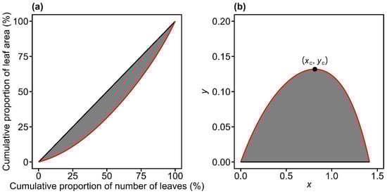
Figure 1. Illustration of the original Lorenz curve (red curve in panel a) and its rotated and right-shifted transformation (red curve in panel b) for leaf area distribution. In panel (a), the Lorenz curve plots the cumulative proportion of leaf area against the cumulative proportion of leaf number. In panel (b), the curve from (a) is rotated 135° counterclockwise around the origin and shifted rightward by $\sqrt{2}$ units. The Gini coefficient is defined as twice the shaded area between the red curve and the line of equality in panel (a). The point of (x_c, y_c) is the maximum value point of the curve in panel (b). The Lorenz asymmetry coefficient is defined as $x_c/\sqrt{2}$.

Building on this framework, Lian et al. [22] reported that when a Lorenz curve derived from leaf area distributions is rotated counterclockwise by 135° around the origin and shifted rightward by $\sqrt{2}$ units, its geometry closely resembles that of a thermal performance curve (Figure 1). This inverted U-shaped curve defined between two fixed points (Figure 1b) can be expressed by a nonlinear performance equation [26,27]:

$$y=c\left(1-e^{-K_1\left(x-x_1\right)}\right)\left(1-e^{K_2\left(x-x_2\right)}\right)$$

(1)

where y denotes the jumping distance of the green frog (Rana clamitans Latreille) at body temperature x, and c, K₁, K₂, x₁, and x₂ are parameters to be estimated. By converting the cumulative Lorenz representation into an inverted U-shaped curve defined within a bounded domain, it allows the application of the performance equation originally developed for biological response curves. Moreover, the transformation reduces the strong autocorrelation inherent in cumulative data and makes prediction errors more readily observable, thereby facilitating statistical modeling and model comparison [22]. The nonlinear performance equation (i.e., Equation (1)), together with its generalized version, has been successfully used to fit the rotated and right-shifted Lorenz curves of leaf area distributions [22,24,28]. In addition, several other nonlinear Lorenz equations have been proposed and widely used to characterize inequality in biological and non-biological size distributions [29,30,31]. However, the performance equation differs from traditional Lorenz equations in that they require a geometric transformation of the data (rotation and translation), whereas conventional Lorenz equations do not. As a result, very few studies have directly compared the relative performance of these two classes of equations in quantifying inequality in biological size distributions. Moreover, most previous studies have primarily emphasized the goodness of fit while giving little attention to evaluating the appropriateness of these nonlinear models in terms of their underlying assumptions, such as linear approximations.

To address these gaps, we digitized all foliage leaves from 121 culms of Semiarundinaria densiflora (Rendle) T. H. Wen, with each culm bearing between 36 and 187 foliage leaves, to determine the area of every individual leaf. We then employed five nonlinear equations (see Section 2.2) to fit the rotated and right-shifted Lorenz curves of leaf area distributions (i.e., cumulative proportion of leaf area versus cumulative proportion of leaf number). Our aim was to assess the relative performance of these equations using multiple evaluation criteria and to provide guidance for the application of Lorenz-based methods in future studies of the inequality of plant organ size distributions.

2. Materials and Methods

2.1. Leaf Collection and Data Acquisition

In October 2024, a total of 121 healthy culms of Semiarundinaria densiflora were randomly collected from the Whitehorse Experimental Station of Nanjing Forestry University, Nanjing, China (119°09′14″ E, 31°36′48″ N). This species, with its abundant and measurable leaves per culm (ranging from 36 to 187 leaves in our study), serves as an ideal system for quantifying inequality in organ size distributions and examining the ecological strategies underlying leaf allocation patterns. To preserve leaf fresh weight and prevent morphological deformation, each culm was cut at ground level, immediately wrapped in moist paper, and transported to the laboratory within two hours. An example of the aboveground portion of a culm is shown in Figure 2.

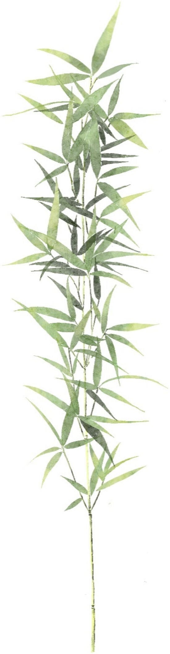
Figure 2. Hand-drawn illustration of the aboveground portion of Semiarundinaria densiflora (Rendle) T. H. Wen.

All foliage leaf blades were removed from each culm and scanned using a flatbed scanner (V550, Epson Indonesia, Batam, Indonesia) at a resolution of 600 dpi. The scanned images were saved in JPG format and subsequently converted into black and white images using Adobe Photoshop 2021 (version 22.4.2; Adobe, San Jose, CA, USA) before being exported as BMP files. Planar boundaries of each leaf were extracted with a custom MATLAB script (version ≥ 2009a; MathWorks, Natick, MA, USA), following the methodology described by Shi et al. [32] and Su et al. [33]. Leaf area was then calculated for each leaf using the “bilat” function in the “biogeom” package (version 1.3.6) [34]. The raw leaf area data are available in Supplementary Table S1 of Jiao et al. [35]. Lorenz curve coordinates for each culm of S. densiflora used for model fitting are available in Table S1.

2.2. Models to Fit the Lorenz Curve

We employed five nonlinear models (two performance equation models and three other traditional Lorenz equation models) to describe the inequality of leaf area distribution of S. densiflora:

(i) The performance equation (Equation (1)) can be used to fit the rotated and right-shifted Lorenz curves (i.e., curves obtained by rotating the original Lorenz curve 135° counterclockwise around the origin and shifting it rightward by $\sqrt{2}$ units, denoted as RRLC) with $x_1=0$ and $x_2=\sqrt{2}$ [22,24]:

$$y=c\left(1-e^{-K_{1}x}\right)\left(1-e^{K_2\left(x-\sqrt{2}\right)}\right)$$

(2)

In this study, (x, y) denotes an arbitrary coordinate point on the RRLC, and c, K₁, and K₂ are parameters to be estimated. Equation (2) was denoted as PE.

(ii) The generalized performance equation extends PE by introducing two additional parameters (a and b), thereby increasing the flexibility of data fitting [22,24]. This generalized version was denoted as GPE:

$$y=c{\left(1-e^{-K_{1}x}\right)}^a{\left(1-e^{K_2\left(x-\sqrt{2}\right)}\right)}^b$$

(3)

where (x, y) in Equation (3) denotes an arbitrary coordinate point on the RRLC, and c, K₁, K₂, a, and b are parameters to be estimated.

(iii) The Sarabia equation (denoted as SarabiaE hereinafter) [23,30]:

$$y_L=\left(1-\mathrm{\lambda }+\mathrm{\eta }\right)x_L+\mathrm{\lambda }{x}_L^{a_1+1}-\mathrm{\eta }\left[1-{\left(1-x_L\right)}^{a_2+1}\right]$$

(4)

where (x_L, y_L) in Equation (4) denotes an arbitrary coordinate point on the original Lorenz curve, and λ, η, a₁, and a₂ are constants to be estimated, where a₁ ≥ 0, a₂ + 1 ≥ 0, ηa₂ + λ ≤ 1, λ ≥ 0, and ηa₂ ≥ 0.

(iv) The Sarabia–Castillo–Slottje equation (denoted as SCSE hereinafter) [29]:

$$y_L=x_L^{\mathrm{\gamma }}{\left[1-{\left(1-x_L\right)}^{\mathrm{\alpha }}\right]}^{\mathrm{\beta }}$$

(5)

where (x_L, y_L) in Equation (5) denotes an arbitrary coordinate point on the original Lorenz curve, and α, β, and γ are constants to be estimated, where 0 < α ≤ 1, β ≥ 1, and γ ≥ 0.

(v) The Sitthiyot–Holasut equation (denoted as SHE hereinafter) [31]:

$$y_L=\left(1-\mathrm{\rho }\right)\left[\left({\displaystyle \frac{2}{P+1}}\right)\left({\displaystyle \frac{x_L-\mathsf{\delta }}{1-\mathsf{\delta }}}\right)\right]+\mathrm{\rho }\left[\left(1-\mathrm{\omega }\right){\left({\displaystyle \frac{x_L-\mathsf{\delta }}{1-\mathsf{\delta }}}\right)}^P+\mathrm{\omega }\left\{1-{\left[1-\left({\displaystyle \frac{x_L-\mathsf{\delta }}{1-\mathsf{\delta }}}\right)\right]}^{{\displaystyle \frac{1}{P}}}\right\}\right]$$

(6)

when $x_L>\mathsf{\delta }$; and $y_L=0$, when $x_L\le \mathsf{\delta }$. (x_L, y_L) in Equation (6) denotes an arbitrary coordinate point on the original Lorenz curve, and δ, ρ, ω, and P are constants to be estimated, where 0 ≤ δ < 1, 0 ≤ ρ ≤ 1, 0 ≤ ω ≤ 1, and P ≥ 1. It is worth noting that SHE is a universal model for fitting Lorenz curves and is particularly suitable for cases of extreme inequality in size distributions [31]. For example, the top 10% of mammal species by body mass account for approximately 99% of the total mammalian biomass, illustrating an extreme concentration pattern [36].

The five nonlinear models selected in this study represent two distinct classes: the performance equations (PE and GPE) are specifically designed to fit the RRLSs, capturing their unimodal and asymmetric features, whereas the traditional Lorenz equations (SarabiaE, SCSE, and SHE) are parametric models widely used in economics to fit original Lorenz curves and are capable of flexibly capturing various distribution shapes. Including both classes enables a comprehensive comparison of their relative performance in quantifying inequality in biological size distributions.

2.3. Data Fitting and Model Evaluation

We used the PE, GPE, SarabiaE, SCSE, and SHE to fit the empirical data of S. densiflora for quantifying the inequality of leaf area distribution. For model comparison, the rotated and right-shifted data were used to fit the PE and GPE, whereas the same transformed data were used to fit the rotated and right-shifted forms of the SarabiaE, SCSE, and SHE models. Model parameters were estimated by minimizing the residual sum of squares (RSS) between observed and predicted y-values using the Nelder–Mead optimization algorithm [37].

The root-mean-square error (RMSE) was employed to quantify the goodness of fit for each model, with smaller RMSE values indicating higher predictive accuracy. The Akaike information criterion (AIC) was used to evaluate the trade-off between model fit and structural complexity, where lower AIC values indicate better model performance [38]. Pairwise t-tests were conducted to assess the statistical significance of differences in RMSE or AIC values among models.

The foundation of parameter estimation by least squares in nonlinear regression—and many of the associated inference techniques—relies on a first-order Taylor series expansion that locally approximates a nonlinear function by a linear one. This linearization entails two key assumptions: the planar assumption and the uniform coordinate assumption [39,40]. To assess the adequacy of these assumptions, a variety of nonlinearity measures have been proposed, including those based on confidence region distortions [41], estimator bias [42], skewness [43], and kurtosis [44]. Among these, the root-mean-square relative curvature measures (${\mathrm{\gamma }}_{\mathrm{RMS}}$) provide a comprehensive framework for evaluating whether a nonlinear regression model behaves as “close-to-linear” or “far-from-linear” [39,45]. These include the root-mean-square relative intrinsic curvature (${\mathrm{\gamma }}_{\mathrm{RMS}}^N$), which reflects deviations from the planar assumption, and the root-mean-square relative parameter–effects curvature (${\mathrm{\gamma }}_{\mathrm{RMS}}^T$), which reflects deviations from the uniform coordinate assumption. A model classified as “close-to-linear” implies that its least squares estimators closely adhere to the desirable asymptotic properties of linear regression—namely being unbiased, approximately normally distributed, and achieving minimum variance [46,47]. In contrast, “far-from-linear” models fail to meet these properties, limiting the reliability of inference. The evaluation of ${\mathrm{\gamma }}_{\mathrm{RMS}}^N$ and ${\mathrm{\gamma }}_{\mathrm{RMS}}^T$ is benchmarked against a critical curvature value (K_c), defined as $1/\sqrt{F\left(m,n-m;{\alpha }_0\right)}$, where F represents the F-distribution, m is the number of model parameters, n is the number of data points, and ${\alpha }_0=0.05$ is the significance level [39]. If ${\mathrm{\gamma }}_{\mathrm{RMS}}^N<K_c$, the planar assumption is considered valid, whereas ${\mathrm{\gamma }}_{\mathrm{RMS}}^T<K_c$ indicates that the uniform coordinate assumption is satisfied.

However, ${\mathrm{\gamma }}_{\mathrm{RMS}}^N$ and ${\mathrm{\gamma }}_{\mathrm{RMS}}^T$ offer limited resolution regarding the performance of individual parameters under the linear approximation. To address this limitation, we complemented our analysis with parameter-specific diagnostics by calculating the skewness (S_k) of each parameter estimator, which reflects the degree of nonlinearity associated with a given parameter [43,44,48]. As a general guideline, nonlinear models can be regarded as “close-to-linear” when the absolute value of S_k is less than 0.25 [47]. Under this condition, the estimators for individual parameters are expected to exhibit desirable asymptotic properties, including approximate unbiasedness, near-normality, and minimal variance [47].

2.4. Quantification of the Asymmetry of the Lorenz Curve and the Gini Coefficient

We used the Lorenz asymmetry coefficient (LAC) to quantify the degree of asymmetry of the RRLC [25,49]:

$$\mathrm{LAC}={\displaystyle \frac{x_c}{\sqrt{2}}}$$

(7)

where x_c represents the x-coordinate associated with the maximum value point on the RRLC (Figure 1b). When LAC > 0.5, the RRLC is left-skewed, indicating an inequality pattern driven by abundant large individuals; when LAC < 0.5, the RRLC is right-skewed, indicating inequality primarily driven by a few large individuals; when LAC = 0.5, the RRLC is bilaterally symmetrical about the vertical line x = x_c, reflecting parity in the contributions of small and large individuals to the overall size distribution [25,49].

By definition, the Gini coefficient is the ratio of the area between the Lorenz curve and the line of absolute equality to the total area beneath the line of absolute equality (Figure 1a). When the Lorenz curve is rotated 135° counterclockwise around the origin and shifted rightward by $\sqrt{2}$ units, it transforms into a parabolic-like curve passing through the fixed points (0, 0) and (0, $\sqrt{2}$) (Figure 1b). After this transformation, the line of absolute equality coincides with the x-axis, and the Gini coefficient (GC) can be expressed as twice the definite integral of the RRLC between the two fixed points [22]:

$$\mathrm{GC}=2\times {\displaystyle {\int }_0^{\sqrt{2}}f(x)dx}$$

(8)

where f(x) in Equation (8) denotes the rotated and right-shifted Lorenz equation.

Model parameters for the five nonlinear equations (PE, GPE, SarabiaE, SCSE, and SHE) were determined using the “fitLorenz” function in the “biogeom” package (version 1.4.4) [34]. This function is designed for fitting Lorenz curves and can be applied to several nonlinear models. Parameter estimation in “fitLorenz” was performed through nonlinear optimization, and the algorithm employed was the Nelder–Mead simplex method [37]. Nonlinearity curvature measures, including ${\mathrm{\gamma }}_{\mathrm{RMS}}^N$, ${\mathrm{\gamma }}_{\mathrm{RMS}}^T$, K_c, and S_k, were computed with the “curvIPEC” and “skewIPEC” functions in the “IPEC” package (version 1.1.0) [50]. All statistical analyses and graphical outputs were performed in R (version 4.3.3) [51].

3. Results

All five models (PE, GPE, SarabiaE, SCSE, and SHE) effectively described the inequality of leaf area distributions, as indicated by RMSE values lower than 0.01 for all cases (Tables S2–S6 in the Supplementary Materials). Pairwise t-tests at the 0.05 significance level revealed that GPE exhibited significantly lower RMSE and AIC values than the other models. PE and SarabiaE work the second best but still outperformed SCSE and SHE (Figure 3). These results demonstrated that, compared with the other four nonlinear models, GPE not only provided the best goodness of fit but also achieved the most favorable trade-off between model complexity and fit quality. Figure 4 illustrates the fitting results for one representative sample of both the original and the rotated and right-shifted Lorenz curves using the five equations.

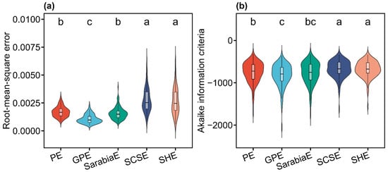
Figure 3. Violin plots showing the distribution of the root-mean-square error (a) and Akaike information criterion (b) values derived from the five Lorenz-based models (PE, GPE, SarabiaE, SCSE, and SHE). The horizontal bar within each box denotes medians; the bottoms and tops of boxes represent the 25th and 75th percentiles, and lines extend to the 1.5-fold interquartile range. Pairwise t-tests were conducted at the 0.05 significance level, with different letters indicating significant differences among models.

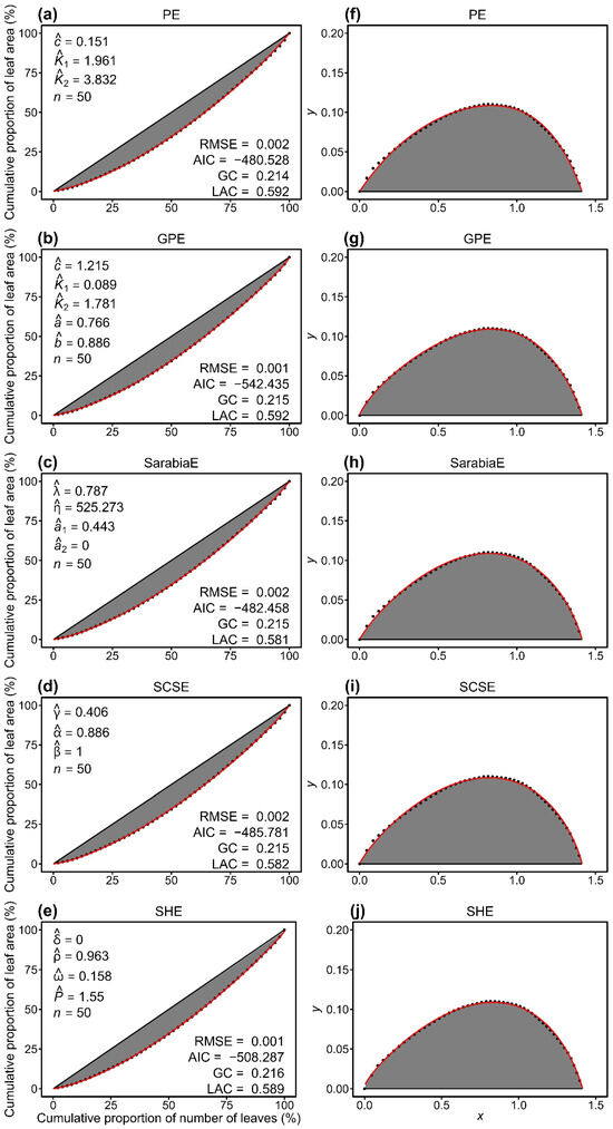
Figure 4. Comparison of the observed (closed circles) and predicted (red lines) data of the original Lorenz curve (a–e) and its rotated and right-shifted version (f–j) for a representative individual culm of Semiarundinaria densiflora. PE and GPE represent the performance equation and its generalized version, respectively. SarabiaE, SCSE, and SHE denote the Sarabia equation, the Sarabia–Castillo–Slottje equation, and the Sitthiyot–Holasut equation, respectively. Letters c, K₁, K₂, a, b, λ, η, a₁, a₂, γ, α, β, δ, ρ, ω, and P with hats represent the estimated values of the parameters of the corresponding equation in each panel. n represents the number of leaves on this individual culm; RMSE represents the root-mean-square error; AIC represents the Akaike information criterion; GC represents the Gini coefficient. LAC represents the Lorenz asymmetry coefficient.

To evaluate overall nonlinearity, we calculated the root-mean-square relative curvatures (i.e., ${\mathrm{\gamma }}_{\mathrm{RMS}}^N$, ${\mathrm{\gamma }}_{\mathrm{RMS}}^T$, and K_c) for all models. For all of the empirical data of S. densiflora, the proportions of culms with ${\mathrm{\gamma }}_{\mathrm{RMS}}^N$ values smaller than the corresponding K_c were 100% (PE), 100% (GPE), 23.97% (SarabiaE), 96.69% (SCSE), and 100% (SHE). By contrast, the proportions of ${\mathrm{\gamma }}_{\mathrm{RMS}}^T$ values below K_c were 15.70% (PE), 0% (GPE), 1.65% (SarabiaE), 0% (SCSE), and 100% (SHE) (Figure 5a). These findings indicated that SHE displayed the best linear approximation behavior among the five models, while SarabiaE exhibited the worst. Notably, although PE, GPE, and SCSE satisfied the planar assumption (with nearly all ${\mathrm{\gamma }}_{\mathrm{RMS}}^N$ values smaller than the K_c), they performed poorly with respect to the uniform coordinate assumption, as indicated by less than 16% of ${\mathrm{\gamma }}_{\mathrm{RMS}}^T$ values falling below K_c.

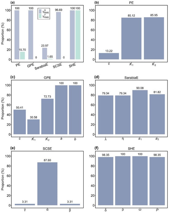
Figure 5. Assessment of the linear approximation behavior of the five equations (PE, GPE, SarabiaE, SCSE, and SHE) at the global (a) and parameter levels (b–f). In panel a, ${\mathrm{\gamma }}_{\mathrm{RMS}}^N$ represents root-mean-square relative intrinsic curvature, and ${\mathrm{\gamma }}_{\mathrm{RMS}}^T$ represents root-mean-square relative parameter-effects curvature. Percentages above the bars indicate the proportions of ${\mathrm{\gamma }}_{\mathrm{RMS}}^N$ or ${\mathrm{\gamma }}_{\mathrm{RMS}}^T$ values smaller than the critical curvature. In (b–f), percentages above the bars indicate the proportions of the absolute values of skewness of each parameter in the corresponding equation less than 0.25.

Parameter-specific skewness (S_k) analysis provided further insights into nonlinear behavior. For PE, the absolute values of S_k for parameters c, K₁, and K₂ were smaller than 0.25 in 13.22%, 85.12%, and 85.95% of cases, respectively (Figure 5b). For GPE, the proportions of the absolute values of S_k below 0.25 were 50.41% (c), 30.58% (K₁), 72.73% (K₂), and 100% for both a and b (Figure 5c). In SarabiaE, 79.34%, 79.34%, 90.08%, and 81.82% of the absolute values of S_k for λ, η, a₁, and a₂ were smaller than 0.25 (Figure 5d). For SCSE, the proportions were 3.31% (γ), 87.60% (α), and 3.31% (β) (Figure 5e). For SHE, nearly all values were smaller than 0.25, with 98.35% (δ), 100% (ρ), 100% (ω), and 98.35% (P) (Figure 5f). Collectively, these results confirmed that SHE demonstrated the strongest close-to-linear behavior, with nearly all of the absolute values of S_k for each parameter being smaller than 0.25. PE also showed relatively good close-to-linear behavior, except for parameter c, where fewer than 14% of the absolute values of S_k were less than 0.25. By contrast, SCSE performed the worst, with two parameters (γ and β) having less than 4% of the absolute values of S_k below 0.25.

The mean (±standard deviation) values of the Lorenz asymmetry coefficient (LAC) were 0.571 ± 0.023 for PE, 0.569 ± 0.027 for GPE, 0.565 ± 0.019 for SarabiaE, 0.570 ± 0.018 for SCSE, and 0.576 ± 0.017 for SHE (Tables S2–S6). The consistency of LAC values across the five models indicated that relatively abundant, larger leaves disproportionately contribute to the inequality in leaf area distribution across the 121 culms.

4. Discussion

4.1. Applications of the Rotated and Right-Shifted Lorenz Curves (RRLCs) in Ecology

The distribution of individual sizes, such as organ dimensions, provides an important window into species’ physiological adaptations, ecological strategies, and evolutionary dynamics [52,53,54]. At the population level, the frequency distribution of individual sizes often reflects the combined effects of resource competition and density dependence. For example, the negative relationship between mean individual size and population density in plants is well captured by the self-thinning law: as density increases, competition for limited resources intensifies, smaller individuals die, and the surviving individuals attain larger average sizes [53]. This trade-off highlights the role of spatial limitation and resource allocation in regulating growth and survival. Moreover, temporal shifts in size distributions can serve as indicators of ecosystem resilience, defined as the capacity to withstand and recover from environmental perturbations [55,56,57]. For instance, an increase in the Gini coefficient of leaf size under drought stress reflects intensified inequality in resource allocation, whereas a more homogeneous distribution may indicate greater community stability [21]. In ecological studies, the Gini coefficient has thus been widely applied to quantify inequality in the allocation of resources among individuals, such as light, water, or nutrients, thereby providing a proxy for competitive asymmetry within populations [52,58].

From an ecological perspective, the use of RRLCs substantially broadens the application of inequality metrics. For instance, the Gini coefficient (calculated by Equation (8)) derived from RRLCs not only provides a more tractable geometric form but also largely eliminates the autocorrelation inherent in cumulative data. Such approaches can be employed to compare organ size distributions among species with contrasting ecological strategies, to assess how environmental gradients (e.g., moisture availability or light conditions) influence within-population trait inequality, and to explore evolutionary trade-offs in resource allocation.

4.2. Ecological Perspectives on Lorenz Asymmetry in Leaf Area Distributions

The Lorenz asymmetry coefficient (LAC) derived from the RRLC complements the Gini coefficient by explicitly incorporating the contribution of large-sized individuals to overall inequality. In this study, most RRLCs were left-skewed (LAC > 0.5), highlighting the predominant contribution of larger leaves to the inequality of leaf area distributions of S. densiflora shoots. One possible explanation is the adaptive adjustment of leaf morphology in response to heterogeneous microenvironments. Consistent with a previous study, Chen et al. [49] found that most RRLCs of the leaf area of Shibataea chinensis Nakai exhibited left skewness, which could be interpreted as a consequence of adaptive strategies for optimizing light capture under shaded or heterogeneous light conditions. In understory or lower canopy environments where light availability is reduced, plants typically develop larger, thinner leaves to maximize intercepted light [59,60].

When LAC equals 0.5, the Lorenz curve is symmetrical, indicating parity in contributions between smaller and larger leaves and a relatively smooth curvature. As LAC deviates from 0.5, inequality becomes increasingly influenced by larger leaves, and the curve develops steeper, asymmetric segments [49]. Such curvature differences may reflect underlying allocation strategies. If carbon investment disproportionately favors particular leaf cohorts (e.g., more light-exposed leaves), cumulative leaf area increases rapidly with leaf number, producing steeper curvature. Conversely, a more uniform allocation yields flatter and more symmetrical curves.

The Lorenz asymmetry coefficient addresses a key limitation of the Gini coefficient, which is insensitive to the asymmetry of the Lorenz curve. By distinguishing whether inequality is primarily driven by many moderately large individuals or by a few exceptionally large ones, the Lorenz asymmetry coefficient provides additional ecological insight into the structure of size distributions. Furthermore, integrating Lorenz-based indices, including both the Gini coefficient and the Lorenz asymmetry coefficient, with measures of community stability or ecosystem resilience may yield new perspectives on how inequality in organ size distributions mediates ecological responses to environmental change.

4.3. The Importance of Nonlinearity Curvature Measures in Model Evaluation

In nonlinear regression, root-mean-square error (RMSE) and Akaike information criterion (AIC) are widely used criteria for model evaluation. However, these indices alone are insufficient because they overlook the stochastic assumptions underlying nonlinear regression models [39]. Specifically, it is essential to assess whether parameter estimates exhibit close-to-linear behavior, as such estimates tend to possess desirable asymptotic properties: approximate unbiasedness, normality, and minimum variance [46,47]. If the close-to-linear assumption is violated, the statistical properties of the parameter estimates may deteriorate. In such cases, the least squares estimators may deviate from these desirable asymptotic characteristics, potentially leading to biased parameter estimates, unreliable confidence intervals, and difficulties in conducting valid hypothesis testing.

Our analysis highlighted the trade-offs among different Lorenz equation models in terms of fitting performance and linear approximation behavior. Among the five models, GPE achieved the best goodness of fit (Figure 3). Moreover, GPE robustly satisfied the planar assumption, with all ${\mathrm{\gamma }}_{\mathrm{RMS}}^N$ values smaller than the corresponding K_c. Nevertheless, it failed to meet the uniform coordinate assumption, as all ${\mathrm{\gamma }}_{\mathrm{RMS}}^T$ values exceeded the corresponding K_c (Figure 5a). At the parameter level, GPE also showed drawbacks: two of its key parameters (c and K₁) did not demonstrate close-to-linear characteristics according to skewness analysis (Figure 5c). At the other end of the spectrum, SHE provided the poorest fit to the observed data (Figure 3), yet it displayed the best linear approximation. All of its ${\mathrm{\gamma }}_{\mathrm{RMS}}^N$ and ${\mathrm{\gamma }}_{\mathrm{RMS}}^T$ values were below the corresponding K_c (Figure 5a), and nearly all parameter estimates exhibited close-to-linear behavior based on skewness (Figure 5f).

The contrasting performance of GPE and SHE underscores an important point: relying solely on goodness-of-fit measures such as RMSE or AIC may provide an incomplete or even misleading picture of model performance, particularly for complex nonlinear models with multiple parameters [48]. Without considering nonlinearity curvature, one risks overlooking violations of the underlying stochastic assumptions when estimating parameters via least squares protocols. Therefore, future studies should evaluate nonlinear models not only in terms of their fitting performance but also with respect to curvature-based diagnostics, ensuring that both predictive accuracy and statistical validity are properly balanced. For other plant species, the relative performance of these models may vary depending on the degree of inequality, sample size, and the underlying distribution of leaf areas. Species with extreme inequality may be better fitted by SHE, while those with more uniform distributions may be adequately described by GPE. Therefore, model selection should be guided by both the mathematical properties of the models and the empirical characteristics of the data.

In addition, it remains unclear whether curvature-based diagnostics themselves are sensitive to environmental gradients that shape the empirical distributions being modeled. As environmental heterogeneity, such as variation in light availability or hydraulic conditions, can influence organ size distributions, it is conceivable that these factors may indirectly affect the stability and linear approximation behavior of nonlinear models. Addressing this possibility will require multi-site or environmentally stratified datasets that explicitly incorporate contrasting ecological conditions. Such efforts would help clarify whether model diagnostic behavior is purely a statistical property or partially reflects environmentally mediated variation in underlying biological structure.

5. Conclusions

In this study, we comprehensively evaluated the performance of five nonlinear models (PE, GPE, SarabiaE, SCSE, and SHE) in fitting the rotated and right-shifted Lorenz curves to describe the empirical data of leaf area distribution in S. densiflora. Our results revealed a clear trade-off among model performance criteria. GPE and SHE represented opposite ends of the performance spectrum: the former maximized predictive accuracy but compromised linear approximation properties, whereas the latter favored close-to-linear behavior at the expense of fit. These findings underscore that predictive accuracy alone is insufficient for evaluating nonlinear regression models. Instead, it is also necessary to examine the linear approximation behavior of model parameters, particularly when dealing with complex models with multiple parameters.

The analytical framework developed in this study, integrating model fitting, curvature-based diagnostics, and Lorenz asymmetry assessment, is not restricted to S. densiflora or to leaf area distributions. It can be extended to other plant species and additional organs (e.g., fruits, seeds, or stomata), where size inequality may reflect underlying ecological and physiological regulation. More generally, the framework is applicable to biological systems characterized by size–frequency or allocation distributions, such as body size structure within animal populations or biomass partitioning within communities. By providing a standardized method to evaluate both predictive accuracy and statistical validity, our framework offers a generalizable tool for studying inequality across diverse biological hierarchies and environmental contexts.

References

- Poorter, L.; Bongers, F. Leaf traits are good predictors of plant performance across 53 rain forest species. Ecology 2006, 87, 1733–1743. [Google Scholar] [CrossRef]
- Rascher, U.; Nedbal, L. Dynamics of photosynthesis in fluctuating light. Curr. Opin. Plant Biol. 2006, 9, 671–678. [Google Scholar] [CrossRef]
- Wright, I.J.; Reich, P.B.; Westoby, M.; Ackerly, D.D.; Baruch, Z.; Bongers, F.; Cavender-Bares, J.; Chapin, T.; Cornelissen, J.H.C.; Diemer, M.; et al. The worldwide leaf economics spectrum. Nature 2004, 428, 821–827. [Google Scholar] [CrossRef] [PubMed]
- Zirbel, C.R.; Bassett, T.; Grman, E.; Brudvig, L.A. Plant functional traits and environmental conditions shape community assembly and ecosystem functioning during restoration. J. Appl. Ecol. 2017, 54, 1070–1079. [Google Scholar] [CrossRef]
- Duursma, R.A.; Falster, D.S. Leaf mass per area, not total leaf area, drives differences in above-ground biomass distribution among woody plant functional types. New Phytol. 2016, 212, 368–376. [Google Scholar] [CrossRef]
- Funk, J.L.; Cornwell, W.K. Leaf traits within communities: Context may affect the mapping of traits to function. Ecology 2013, 94, 1893–1897. [Google Scholar] [CrossRef]
- Westoby, M. A leaf-height-seed (LHS) plant ecology strategy scheme. Plant Soil 1998, 199, 213–227. [Google Scholar] [CrossRef]
- Milla, R.; Reich, P.B. The scaling of leaf area and mass: The cost of light interception increases with leaf size. Proc. R. Soc. B 2007, 274, 2109–2115. [Google Scholar] [CrossRef]
- Niinemets, U.; Portsmuth, A.; Tena, D.; Tobias, M.; Matesanz, S.; Valladares, F. Do we underestimate the importance of leaf size in plant economics? Disproportional scaling of support costs within the spectrum of leaf physiognomy. Ann. Bot. 2007, 100, 283–303. [Google Scholar] [CrossRef] [PubMed]
- Niklas, K.J.; Cobb, E.D.; Niinemets, U.; Reich, P.B.; Sellin, A.; Shipley, B.; Wright, I.J. “Diminishing returns” in the scaling of functional leaf traits across and within species groups. Proc. Natl. Acad. Sci. USA 2007, 10, 8891–8896. [Google Scholar] [CrossRef] [PubMed]
- Gastwirth, J.L. The estimation of the Lorenz curve and Gini index. Rev. Econ. Stat. 1972, 54, 306–316. [Google Scholar] [CrossRef]
- Gini, C. Measurement of inequality of incomes. Econ. J. 1921, 31, 124–126. [Google Scholar] [CrossRef]
- Lorenz, M.O. Methods of measuring the concentration of wealth. Am. Stat. Assoc. 1905, 9, 209–219. [Google Scholar] [CrossRef]
- Kakwani, N.C. Applications of Lorenz curves in economic analysis. Econometrica 1977, 45, 719–727. [Google Scholar] [CrossRef]
- Drăgulescu, A.; Yakovenko, V.M. Exponential and power-law probability distributions of wealth and income in the United Kingdom and the United States. Physica A 2001, 299, 213–221. [Google Scholar] [CrossRef]
- Aydiner, E.; Cherstvy, A.G.; Metzler, R. Money distribution in agent-based models with position-exchange dynamics: The Pareto paradigm revisited. Eur. Phys. J. B 2019, 92, 104. [Google Scholar] [CrossRef]
- Chen, B.J.; During, H.J.; Vermeulen, P.J.; Anten, N.P. The presence of a below-ground neighbour alters within-plant seed size distribution in Phaseolus vulgaris. Ann. Bot. 2014, 114, 937–943. [Google Scholar] [CrossRef]
- Hara, T. Effects of density and extinction coefficient on size variability in plant populations. Ann. Bot. 1986, 57, 885–892. [Google Scholar] [CrossRef]
- Metsaranta, J.M.; Lieffers, V.J. Inequality of size and size increment in Pinus banksiana in relation to stand dynamics and annual growth rate. Ann. Bot. 2007, 101, 561–571. [Google Scholar] [CrossRef]
- Taylor, K.M.; Aarssen, L.W. Neighbor effects in mast year seedlings of Acer saccharum. Am. J. Bot. 1989, 76, 546–554. [Google Scholar] [CrossRef]
- Huang, L.; Ratkowsky, D.A.; Hui, C.; Gielis, J.; Lian, M.; Yao, W.; Li, Q.; Zhang, L.; Shi, P. Inequality measure of leaf area distribution for a drought-tolerant landscape plant. Plants 2023, 12, 3143. [Google Scholar] [CrossRef]
- Lian, M.; Shi, P.; Zhang, L.; Yao, W.; Gielis, J.; Niklas, K.J. A generalized performance equation and its application in measuring the Gini index of leaf size inequality. Trees 2023, 37, 1555–1565. [Google Scholar] [CrossRef]
- Shi, P.; Deng, L.; Niklas, K.J. Rotated Lorenz curves of biological size distributions follow two performance equations. Symmetry 2024, 16, 565. [Google Scholar] [CrossRef]
- Wang, L.; He, K.; Hui, C.; Ratkowsky, D.A.; Yao, W.; Lian, M.; Wang, J.; Shi, P. Comparison of four performance models in quantifying the inequality of leaf and fruit size distribution. Ecol. Evol. 2024, 14, e11072. [Google Scholar] [CrossRef] [PubMed]
- Yao, W.; Niinemets, Ü.; Niklas, K.J.; Damgaard, C.F.; Shi, P. Low size inequality in stomatal area distributions detected for 12 tree and shrub Magnoliaceae species: Evidence of hydraulic optimization. Bot. Lett. 2025, 173, 72–84. [Google Scholar] [CrossRef]
- Huey, R.B. Ecology of Lizard Thermoregulation; Harvard University: Cambridge, MA, USA, 1975. [Google Scholar]
- Huey, R.B.; Stevenson, R.D. Integrating thermal physiology and ecology of ectotherms: A discussion of approaches. Am. Zool. 1979, 19, 357–366. [Google Scholar] [CrossRef]
- Deng, L.; He, K.; Niklas, K.J.; Shi, Z.; Mu, Y.; Shi, P. Comparison of five equations in describing the variation of leaf area distributions of Alangium chinense (Lour.) Harms. Front. Plant Sci. 2024, 15, 1426424. [Google Scholar] [CrossRef]
- Sarabia, J.M.; Castillo, E.; Slottje, D.J. An ordered family of Lorenz curves. J. Econom. 1999, 91, 43–60. [Google Scholar] [CrossRef]
- Sarabia, J.M. A hierarchy of Lorenz curves based on the generalized Tukey’s lambda distribution. Econom. Rev. 1997, 16, 305–320. [Google Scholar] [CrossRef]
- Sitthiyot, T.; Holasut, K. A universal model for the Lorenz curve with novel applications for datasets containing zeros and/or exhibiting extreme inequality. Sci. Rep. 2023, 13, 4729. [Google Scholar] [CrossRef] [PubMed]
- Shi, P.; Ratkowsky, D.A.; Li, Y.; Zhang, L.; Lin, S.; Gielis, J. A general leaf area geometric formula exists for plants—Evidence from the simplified Gielis equation. Forests 2018, 9, 714. [Google Scholar] [CrossRef]
- Su, J.; Niklas, K.J.; Huang, W.; Yu, X.; Yang, Y.; Shi, P. Lamina shape does not correlate with lamina surface area: An analysis based on the simplified Gielis equation. Glob. Ecol. Conserv. 2019, 19, e00666. [Google Scholar] [CrossRef]
- Shi, P.; Gielis, J.; Quinn, B.K.; Niklas, K.J.; Ratkowsky, D.A.; Schrader, J.; Ruan, H.; Wang, L.; Niinemets, Ü. ‘biogeom’: An R package for simulating and fitting natural shapes. Ann. N. Y. Acad. Sci. 2022, 1516, 123–134. [Google Scholar] [CrossRef]
- Jiao, Z.; Liu, S.; Niklas, K.J.; Damgaard, C.F.; Yao, W.; Lian, M.; Jiang, F.; Shi, P. Linking the Weibull distribution to Gini coefficients: A bamboo specific framework for intra-culm leaf area inequality. Front. Plant Sci. 2025, 16, 1685552. [Google Scholar] [CrossRef]
- Smith, F.A.; Lyons, S.K.; Ernest, S.K.M.; Jones, K.E.; Kaufman, D.M.; Dayan, T.; Marquet, P.A.; Brown, J.H.; Haskell, J.P. Body mass of late Quaternary mammals. Ecology 2003, 84, 3403. [Google Scholar] [CrossRef]
- Nelder, J.A.; Mead, R. A simplex method for function minimization. Comput. J. 1965, 7, 308–313. [Google Scholar] [CrossRef]
- Spiess, A.N.; Neumeyer, N. An evaluation of R2 as an inadequate measure for nonlinear models in pharmacological and biochemical research: A Monte Carlo approach. BMC Pharmacol. 2010, 10, 6. [Google Scholar] [CrossRef] [PubMed]
- Bates, D.M.; Watts, D.G. Relative curvature measures of nonlinearity. J. R. Stat. Soc. B 1980, 42, 1–16. [Google Scholar] [CrossRef]
- Bates, D.M.; Watts, D.G. Nonlinear Regression Analysis and Its Applications; John Wiley & Sons: New York, NY, USA, 1988. [Google Scholar]
- Beale, E.M.L. Confidence regions in non-linear estimation. J. R. Stat. Soc. B 1960, 22, 41–76. [Google Scholar] [CrossRef]
- Box, M.J. Bias in nonlinear estimation. J. R. Stat. Soc. B 1971, 33, 171–201. [Google Scholar] [CrossRef]
- Hougaard, P. The appropriateness of the asymptotic distribution in a nonlinear regression model in relation to curvature. J. R. Stat. Soc. B 1985, 47, 103–114. [Google Scholar] [CrossRef]
- Haines, L.M.; O’Brien, T.E.; Clarke, G.P.Y. Kurtosis and curvature measures for nonlinear regression models. Stat. Sin. 2004, 14, 547–570. [Google Scholar]
- He, K.; Wang, L.; Ratkowsky, D.A.; Shi, P. Comparison of four light-response models using relative curvature measures of nonlinearity. Sci. Rep. 2024, 14, 24058. [Google Scholar] [CrossRef]
- Ratkowsky, D.A. Nonlinear Regression Modeling: A Unified Practical Approach; Marcel Dekker: New York, NY, USA, 1983. [Google Scholar]
- Ratkowsky, D.A. Handbook of Nonlinear Regression Models; Marcel Dekker: New York, NY, USA, 1990. [Google Scholar]
- Ratkowsky, D.A.; Reddy, G.V.P. Empirical model with excellent statistical properties for describing temperature-dependent developmental rates of insects and mites. Ann. Entomol. Soc. Am. 2017, 110, 302–309. [Google Scholar] [CrossRef]
- Chen, Y.; Jiang, F.; Damgaard, C.F.; Shi, P.; Weiner, J. Re-expression of the Lorenz asymmetry coefficient on the rotated and right-shifted Lorenz curve of leaf area distributions. Plants 2025, 14, 1345. [Google Scholar] [CrossRef]
- Shi, P.; Ridland, P.; Ratkowsky, D.A.; Li, Y. IPEC: Root Mean Square Curvature Calculation. R Package Version 1.1.0. Available online: https://CRAN.R-project.org/package=IPEC (accessed on 14 January 2024).
- R Core Team. R: A Language and Environment for Statistical Computing; R Foundation for Statistical Computing: Vienna, Austria, 2024; Available online: https://www.r-project.org/ (accessed on 1 April 2024).
- Vogel, E.R.; Janson, C.H. Quantifying primate food distribution and abundance for socioecological studies: An objective consumer-centered method. Int. J. Primatol. 2011, 32, 737–754. [Google Scholar] [CrossRef]
- Dillon, K.T.; Henderson, A.N.; Lodge, A.G.; Hamilton, N.I.; Sloat, L.L.; Enquist, B.J.; Price, C.A.; Kerkhoff, A.J. On the relationships between size and abundance in plants: Beyond forest communities. Ecosphere 2019, 10, e02856. [Google Scholar] [CrossRef]
- Diaz, R.M.; Ernest, S.K.M. Temporal changes in the individual size distribution modulate the long-term trends of biomass and energy use of North American breeding bird communities. Glob. Ecol. Biogeogr. 2024, 33, 74–84. [Google Scholar] [CrossRef]
- Dakos, V.; Carpenter, S.R.; van Nes, E.H.; Scheffer, M. Resilience indicators: Prospects and limitations for early warnings of regime shifts. Philos. Trans. R. Soc. B 2015, 370, 20130263. [Google Scholar] [CrossRef]
- Scheffer, M.; Bascompte, J.; Brock, W.A.; Brovkin, V.; Carpenter, S.R.; Dakos, V.; Held, H.; van Nes, E.H.; Rietkerk, M.; Sugihara, G. Early-warning signals for critical transitions. Nature 2009, 461, 53–59. [Google Scholar] [CrossRef]
- Van Meerbeek, K.; Jucker, T.; Svenning, J.C. Unifying the concepts of stability and resilience in ecology. J. Ecol. 2021, 109, 3114–3132. [Google Scholar] [CrossRef]
- Walker, G.K.; Blackshaw, R.E.; Dekker, J. Leaf area and competition for light between plant species using direct sunlight transmission. Weed Technol. 1988, 2, 159–165. [Google Scholar] [CrossRef]
- Niinemets, Ü. Global-scale climatic controls of leaf dry mass per area, density, and thickness in trees and shrubs. Ecology 2001, 82, 453–469. [Google Scholar] [CrossRef]
- de Casas, R.R.; Vargas, P.; Pérez-Corona, E.; Manrique, E.; García-Verdugo, C.; Balaguer, L. Sun and shade leaves of Olea europaea respond differently to plant size, light availability and genetic variation. Funct. Ecol. 2011, 25, 802–812. [Google Scholar] [CrossRef]
Disclaimer/Publisher’s Note: The statements, opinions and data contained in all publications are solely those of the individual author(s) and contributor(s) and not of MDPI and/or the editor(s). MDPI and/or the editor(s) disclaim responsibility for any injury to people or property resulting from any ideas, methods, instructions or products referred to in the content. |
© 2026 by the authors. Licensee MDPI, Basel, Switzerland. This article is an open access article distributed under the terms and conditions of the Creative Commons Attribution (CC BY) license.