Stability and Forward Bifurcation Analysis of an SI_PIVR Model for Poliovirus Transmission with Neural Network

Abstract

The aim of this research is to formulate and analyze a modified $S{I}_{p}IVR$ mathematical model to study the transmission dynamics of poliovirus and assess the impact of vaccination on disease control. The proposed model extends classical SEIV-type frameworks by incorporating a recovered compartment with long-term immunity and by replacing the traditional exposed class with a pre-infectious compartment ($I_p$) that captures silent viral shedding during the incubation phase of poliovirus. This modification addresses the critical epidemiological feature that individuals can transmit the virus before showing symptoms while maintaining biological accuracy in compartment definition. Several fundamental analytical properties are rigorously established, including positivity, boundedness, and the existence of a biologically meaningful invariant region. The basic reproduction number $R_0$ is derived using the next-generation matrix approach, and comprehensive stability analysis is carried out. The analysis shows that the DFE is locally and globally asymptotically stable whenever $R_0<1$. Using center manifold theory, a forward bifurcation is rigorously demonstrated, indicating that disease persistence emerges smoothly as $R_0$ crosses unity. Local and global sensitivity analyses of the basic reproduction number $R_0$ identify critical epidemiological parameters, and points to vaccination coverage and transmission rates as key drivers of outbreak dynamics. Numerical simulations confirm the analytical results and illustrates two different epidemiological scenarios, one with $R_0<1$, and another with $R_0>1$ along with neural network analysis by using the same data from both cases in a built-in function package in MATLAB-2020 software. It utilizes all of its hidden layers to check the data used by the model for validation performance and training and to find the absolute and mean squared errors. It also shows how vaccination suppresses the spread of infection. These findings provide a strong mathematical basis for public health policy, offering strategic insight into how vaccination campaigns might be optimized to accelerate progress toward global polio eradication.

1. Introduction

Poliomyelitis, more commonly referred to as polio, is a highly infectious viral disease caused by the poliovirus, which primarily invades the nervous system and can result in irreversible paralysis [1]. Historical evidence for the presence of polio dates back to ancient Egyptian artifacts that showed typical depictions of limb deformities [2]. However, polio emerged as a major epidemic disease during the late 19th and early 20th centuries, paradoxically at a time when marked improvements in sanitation and public health were occurring [3]. This feature led to the categorization of polio as a “disease of development,” as improved hygiene reduced early-life exposure to the virus, thus increasing the number of susceptible adolescents and adults who were at a higher risk of severe neurological complications if infected. The mid-20th century saw devastating outbreaks, particularly in industrialized nations, which motivated intensive scientific efforts, and culminated in the inactivated polio vaccine (IPV) invented by Jonas Salk and the oral polio vaccine (OPV) invented by Albert Sabin. These breakthroughs changed global public health and gave rise to the current worldwide eradication campaign [4].

Despite remarkable progress, polio remains a global health challenge [5]. Although endemic transmission remains confined to a few regions, international travel, population displacement, and pockets of low immunization coverage continue to create outbreak risks [6]. Furthermore, cVDPVs-emerging due to low vaccination rates in parts of the population—raise a serious reason for further surveillance and sustained immunization efforts [7]. Silent transmission in polio, wherein individuals shed the virus but rarely manifest symptoms, has further complicated eradication efforts. Strong analytical tools are needed to understand the dynamics of viral spread [8]. A particularly insidious feature of poliovirus is its silent transmission: approximately $95\%$ of infections are asymptomatic or mild, yet infected individuals shed the virus and can infect others during the incubation period before showing symptoms [9,10]. This means there exists a significant population of pre-infectious individuals who are actively transmitting the virus while not yet displaying clinical symptoms. Classical compartmental models often represent this period as an exposed (E) class with no transmission, which is epidemiologically inaccurate for polio. To address this, our model replaces the traditional exposed compartment with a pre-infectious compartment ($I_p$) that captures both the incubation period and the asymptomatic transmission that occurs during this phase. This silent spread, combined with the emergence of circulating vaccine-derived polioviruses (cVDPVs) in under-vaccinated populations, complicates surveillance and undermines eradication efforts [11]. Mathematical modeling has become one of the indispensable tools in understanding and combating polio [12,13,14], providing a structured framework for the simulation of transmission dynamics and the evaluation of the impact of interventions. In particular, compartmental models [15], the most representative of which includes the SEIR [16] structure (Susceptible–Exposed–Infectious–Recovered), enable researchers to partition populations and investigate how contact patterns, latency periods, infectiousness, and immunity influence disease propagation [17,18]. Such models have played a key role in identifying some epidemiologically important thresholds, such as the basic reproduction number [19], that define whether an outbreak will grow or fade out [20]. For example, models considering age-structured and sanitation-dependent transmission have provided insight into how improvements in hygiene led to a shift in the average age of infection that drove the emergence of large polio epidemics in high-income countries before vaccines became available [21] and several other noteworthy studies have also been reported in the literature, such as [22,23,24,25,26].

In addition to advancing theoretical insight, mathematical models have played a vital practical role in public health planning and policy-making [27]. Models have helped establish optimal vaccination strategies, including routine immunization, pulse vaccination, and supplementary immunization activities [28]. They allow the examination of additional factors, such as waning immunity, environmental transmission from contaminated water, and the prevalence of asymptomatic carriers [29]. During the global eradication campaign still in progress, models have been at the heart of determining poliovirus importation risks, assessing response strategies against outbreaks, projecting future patterns of transmission, and informing resource deployment by international health agencies [30]. By providing simulations of different scenarios, such as changes in vaccination coverage, the introduction of new vaccines, and the improvement of sanitation, mathematical modeling offers a cost-effective and powerful tool for foreseeing challenges and preparing robust strategies for disease control [31].

Models of classical polio traditionally are segmented into susceptible, exposed, infectious, and vaccinated classes. One such model is the SEIV model of Archana and Agarwal [32], which is given by

$$\begin{array}{cc}\hfill \dot{S}\left(t\right)& =A-\beta SI-r\beta SE-(\mu +\nu )S,\hfill \\ \hfill \dot{E}\left(t\right)& =\beta SI+r\beta SE-(b+\mu +{\nu }_1)E,\hfill \\ \hfill \dot{I}\left(t\right)& =(b+{\nu }_1)E-(\mu +\alpha )I,\hfill \\ \hfill \dot{V}\left(t\right)& =\nu S-\mu V,\hfill \end{array}$$

(1)

where the compartments represent susceptible S, exposed E, infectious I, and vaccinated V individuals. Despite the fact that this model captures important aspects of polio transmission, it does not consider a recovered compartment, whereas, in reality, individuals who recover from an infection usually develop long-term immunity. In reality, poliovirus can be transmitted during the incubation period, as exposed individuals may shed virus before symptoms appear. Moreover, recovered individuals typically acquire long-term immunity. Ignoring these features may underestimate transmission potential and distort predictions of disease persistence.

Biological Motivation and Model Modifications:

To address these gaps, we develop a modified $S{I}_{p}IVR$ model with two key innovations driven by polio-specific epidemiology:

• Recovered compartment ($\mathit{R}$): Including recovered individuals allows us to track long-term immunity dynamics, which is essential for projecting elimination timelines and assessing the impact of waning immunity. In reality, individuals who recover from infection typically develop long-term immunity, and capturing this population is crucial for accurate long-term projections.
• Enhanced force of infection: Unlike classical models that assume no transmission during the incubation period, our force of infection includes transmission from both pre-infectious (${\alpha }_2{I}_p$) and fully infectious (${\alpha }_{1}I$) individuals. This captures the critical role of silent spread and better reflects real-world polio transmission dynamics, where asymptomatic shedding during the pre-infectious phase drives undetected circulation.

These modifications are not merely mathematical exercises—they are biologically motivated by the unique features of poliovirus epidemiology. The inclusion of transmission from exposed individuals is particularly significant, as it addresses a key factor in polio persistence that has been inadequately represented in previous modeling studies.

2. Problem Formulation

In this work, we overcome these limitations and improve biological realism by developing a modified $S{I}_{p}IVR$ model that includes a recovered class R and an improved force of infection that considers transmission from both pre-infectious and infectious individuals.

Hence, in our model the total population $N\left(t\right)$ divided into five subpopulations namely Susceptible $S\left(t\right)$, pre-infectious $I_p\left(t\right)$, Infected $I\left(t\right)$, Vaccinated $V\left(t\right)$, and Recovered $R\left(t\right)$ while the parameters details are given in Table 1 and graphically flowchart is mentioned in Figure 1.

Table 1. Descriptions of Prameters.

Symbol	Meaning
$\Lambda$	Recruitment rate into susceptible population
$\beta$	Rate of transmission from susceptible to pre-infectious
${\alpha }_1$	Rate of transmission due to infectious class
${\alpha }_2$	Transmission rate due to pre-infectious class
$\mu$	Natural mortality rate
$\lambda$	Vaccination rate
$\delta$	Rate of flow from $I_p\left(t\right)$ to $I\left(t\right)$
$\omega$	Disease-induced mortality rate
$\gamma$	rate of recovery in infectious individuals

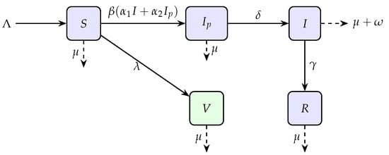
Figure 1. Flow diagram of the $S{I}_{p}IVR$ model illustrating transitions between compartments.

The proposed model is formulated as:

$$\begin{array}{cc}\hfill {\displaystyle \frac{dS}{dt}}& =\Lambda -\beta ({\alpha }_{1}I+{\alpha }_2{I}_p)S-(\mu +\lambda )S,\hfill \\ \hfill {\displaystyle \frac{d{I}_p}{dt}}& =\beta ({\alpha }_{1}I+{\alpha }_2{I}_p)S-(\mu +\delta )I_p,\hfill \\ \hfill {\displaystyle \frac{dI}{dt}}& =\delta I_p-(\mu +\omega +\gamma )I,\hfill \\ \hfill {\displaystyle \frac{dV}{dt}}& =\lambda S-\mu V,\hfill \\ \hfill {\displaystyle \frac{dR}{dt}}& =\gamma I-\mu R,\hfill \end{array}$$

(2)

It is important to note the scope of the present study. Our analysis focuses exclusively on temporal dynamics at the population level using a deterministic compartmental framework. Factors known to be epidemiologically significant for polio—such as age-structured contact patterns, sanitation-dependent transmission, and spatial heterogeneity—are outside the scope of this work. This deliberate scoping decision maintains analytical tractability and allows us to rigorously establish threshold behavior $R_0$, stability properties, and bifurcation patterns. The incorporation of age structure or spatial dynamics would require partial differential equations or agent-based models, which would shift the focus away from the core analytical contributions presented here.

Model Assumptions

The proposed $S{I}_{p}IVR$ model is developed under the following epidemiological and demographic assumptions:

(i)

The total population is assumed to be homogeneous, meaning every individual has an equal probability of coming into contact with any other individual per unit time.

(ii)

Recruitment into the susceptible population occurs at a constant rate $\Lambda$, and all newborns are assumed to be susceptible.

(iii)

Natural mortality occurs at a constant rate $\mu$ in all compartments.

(iv)

The force of infection incorporates transmission from both pre-infectious and infected individuals, recognizing that pre-infectious individuals may contribute to viral shedding and disease spread before showing symptoms.

(v)

Vaccination is administered only to susceptible individuals at a constant rate $\lambda$. Vaccinated individuals acquire permanent immunity and move to the vaccinated compartment V. No waning immunity is considered.

(vi)

Individuals who recover from natural infection develop permanent immunity and move to the recovered compartment R. No waning immunity or reinfection is considered.

(vii)

Disease-induced mortality occurs only in the infectious compartment I at rate $\omega$.

(viii)

All parameters are non-negative and constant over time.

These assumptions provide a biologically plausible yet mathematically tractable framework for analyzing the transmission dynamics of poliovirus and the impact of vaccination strategies.

3. Basic Properties of the Model

Positivity, boundedness, reproduction number, stability analysis, bifurcation analysis, sensitivity analysis, and numerical simulation are covered in this section. Before presenting the said properties of the model, we give some definitions that explore the idea of a neural network (NN) and the need for its application to the said model.

Definition 1 (Neural Network Performance).

In the concept of neural network, the performance refers to the model’s goal achievements in the context of accuracy and best approaches. For the performances, accuracy, mean square error, absolute error, recall, and precision are required for the concerned data. Further, for improvement in performance, the training, networking design, and placement of the hyperparameter should be modified.

Definition 2 (Average Square Error).

The measurement of efficiency is termed the mean square error. It is used for the computation of the mean square deviation between the exact and estimated or Approximate result, which implies the correctness of network predictions.

Definition 3. 

$Mu\left(\mu \right)$ For the rate of learning or step size interval, we usually chose μ. A hyperparameter is used for controlling biases and weight age when the network variation occurs in the learning rate of the training. The rate of learning rate μ refers to the magnitude of step size in loss quantities in optimization techniques under gradient.

3.1. Positivity

Theorem 1. 

The solution of the system at the given initial conditions is always non-negative for $t>0$.

Proof. 

Epidemiological models must be positive to model disease dynamics realistically.

The 1st equation of system (2)

$$\begin{array}{ccc}\hfill {\displaystyle \frac{dS}{dt}}& =& \Lambda -\beta ({\alpha }_{1}I+{\alpha }_2{I}_p)S-(\mu +\lambda )S\hfill \end{array}$$

We have

$$\begin{array}{ccc}\hfill {\displaystyle \frac{dS}{dt}}+[\beta ({\alpha }_{1}I+{\alpha }_2{I}_p)+\mu +\lambda ]S& =& \Lambda \hfill \end{array}$$

The above ODEs are solved by Integrating Factor method with the given Initial condition.

The Integrating Factor is

$$\begin{array}{c}\hfill I.F=e^{{\int }_0^t[\beta ({\alpha }_{1}I+{\alpha }_2{I}_p)+\mu +\lambda ]dt}\end{array}$$

Hence we have

$$S\left(t\right)=\left(S\left(0\right)+{\int }_0^t\Lambda \left(e^{{\int }_0^t[\beta ({\alpha }_{1}I+{\alpha }_2{I}_p)+\mu +\lambda ]dt}\right)\right)e^{-{\int }_0^t[\beta ({\alpha }_{1}I+{\alpha }_2{I}_p)+\mu +\lambda ]dt}$$

$S\left(t\right)$ non-negative for all time $t>0$.

The same approach allows us to show that all other system variables are also non-negative when $t>0$. □

3.2. Boundedness

For the model, the closed set D represents a feasible region.

$$D=\left\{(S,I_p,I,V,R)\in {\mathbb{R}}_{+}^5:N\le {\displaystyle \frac{\Lambda }{\mu }}\right\},$$

Theorem 2. 

The closed set D is bounded and positive invariant.

Proof. 

The total population $N=S+I_p+I+V+R$. Taking derivative

$$\begin{array}{ccc}\hfill {\displaystyle \frac{dN}{dt}}& =& {\displaystyle \frac{d}{dt}}(S+I_p+I+V+R)\hfill \\ & =& \Lambda -\mu S-\mu I_p-\mu I-\mu V-\mu R-\omega I\hfill \\ & =& \Lambda -\mu N-\omega I\hfill \\ & \le & \Lambda -\mu N\hfill \end{array}$$

To simplify, we have

$$N\left(t\right)\le N\left(0\right)e^{-\mu t}+{\displaystyle \frac{\Lambda }{\mu }}(1-e^{-\mu t})$$

As $t\to \infty$, $e^{-\mu t}\to 0$ and so ${lim}_{t\to \infty }N\left(t\right)\le {\displaystyle \frac{\Lambda }{\mu }}$.

Thus, D is bounded and absolutely invariant in ${\mathbb{R}}_{+}^5$. □

3.3. Basic Reproduction Number

Now we calculate the basic threshold number for our proposed problem (2). For this purpose we use next-generation matrix method.

We consider the infectious classes in the proposed model. Let $Y=(I_p,I)$.

$$\begin{array}{c}\hfill \mathbf{f}=\left[\begin{array}{c}\beta ({\alpha }_{1}I+{\alpha }_2{I}_p)S\\ 0\end{array}\right]\mathbf{v}=\left[\begin{array}{c}(\mu +\delta )I_p\\ -\delta I_p+(\mu +\omega +\gamma )I\end{array}\right]\end{array}$$

The Jacobian matrix of $\mathbf{F}$ and $\mathbf{v}$ evaluated at DFE are

$$\begin{array}{c}\hfill \mathbf{f}=\left[\begin{array}{cc}\beta {\alpha }_2{S}^0& \beta {\alpha }_1{S}^0\\ 0& 0\end{array}\right]\mathbf{v}=\left[\begin{array}{cc}(\mu +\delta )& 0\\ -\delta & (\mu +\omega +\gamma )\end{array}\right]\end{array}$$

$$\begin{array}{c}\hfill {\mathit{V}}^{-1}=\left[\begin{array}{cc}{\displaystyle \frac{1}{(\mu +\delta )}}& 0\\ {\displaystyle \frac{\delta }{(\mu +\delta )(\mu +\omega +\gamma )}}& {\displaystyle \frac{1}{(\mu +\omega +\gamma )}}\end{array}\right]\end{array}$$

$$\mathbf{F}{\mathbf{V}}^{-1}=\left[\begin{array}{cc}{\displaystyle \frac{\beta {\alpha }_2{S}^0}{(\mu +\delta )}}+{\displaystyle \frac{\beta {\alpha }_1{S}^0\delta }{(\mu +\delta )(\mu +\omega +\gamma )}}& {\displaystyle \frac{\beta {\alpha }_1{S}^0}{(\mu +\omega +\gamma )}}\\ 0& 0\end{array}\right]$$

The spectral radius of $F{V}^{-1}$ is the threshold number $R_0$:

$$R_0={\displaystyle \frac{\beta {\alpha }_2{S}^0}{(\mu +\delta )}}+{\displaystyle \frac{\beta {\alpha }_1{S}^0\delta }{(\mu +\delta )(\mu +\omega +\gamma )}}$$

Substituting $S^0={\displaystyle \frac{\Lambda }{\mu +\lambda }}$:

$$R_0={\displaystyle \frac{\beta \Lambda ({\alpha }_2(\mu +\omega +\gamma )+{\alpha }_1\delta )}{(\mu +\lambda )(\mu +\delta )(\mu +\omega +\gamma )}}$$

The basic reproduction number $R_0$ represents the average number of secondary infections produced by a single infected individual in a completely susceptible population. Biologically, $R_0<1$ implies that each infected individual replaces itself with less than one new infection, causing the disease to die out. Conversely, $R_0>1$ indicates that each infected individual generates more than one new infection, leading to disease persistence and potential outbreaks as seen in the Figure 2.

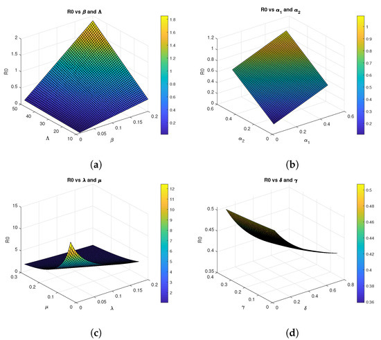
Figure 2. Three-dimensional graphs of $R_0$ for Model 2 using parametrs values $\mu =0.5,\Lambda =1000,\beta =0.002,{\alpha }_1=0.2,$${\alpha }_2=0.15,\lambda =0.6,\delta =0.9,\omega =0.6,\gamma =0.23.$

3.4. Equilibriums Points

3.4.1. Disease Free State

When a community is in a disease-free state (DFS), there is no disease infection. The symbol for it is $E^0$.

The infectious classes are taken to be equal to zero in order to reach this state. We observe that the DFS is given by $E^0=(S^0,0,0,V^0,0).$

$$E^0=\left({\displaystyle \frac{\Lambda }{\mu +\lambda }},0,0,{\displaystyle \frac{\lambda \Lambda }{\mu (\mu +\lambda )}},0\right).$$

3.4.2. Disease Endemic State

$E^{*}=(S^{*},I_p^{*},I^{*},V^{*},R^{*})$ represent the Disease Endemic State which indicates that the infection is present in the population. The endemic equilibrium point for the system (2) is follows:

$$\left\{\begin{array}{cc}\hfill S^{*}& ={\displaystyle \frac{(\mu +\delta )(\mu +\omega +\gamma )}{\beta (\delta {\alpha }_1+{\alpha }_2(\mu +\omega +\gamma ))}},\hfill \\ \hfill I_p^{*}& ={\displaystyle \frac{(\mu +\omega +\gamma )}{\delta }}{I}^{*},\hfill \\ \hfill I^{*}& ={\displaystyle \frac{\delta (\mu +\lambda )(R_0-1)}{\beta ({\alpha }_1\delta +{\alpha }_2(\mu +\omega +\gamma ))}},\hfill \\ \hfill V^{*}& ={\displaystyle \frac{\lambda }{\mu }}{S}^{*}={\displaystyle \frac{\lambda \beta (\delta {\alpha }_1+{\alpha }_2(\mu +\omega +\gamma ))}{\mu (\mu +\delta )(\mu +\omega +\gamma )}},\hfill \\ \hfill R^{*}& ={\displaystyle \frac{\gamma }{\mu }}{I}^{*}.\hfill \end{array}\right.$$

It is clear from this expression that the infectious class $I^{*}$ depends explicitly on the basic reproduction number $R_0$. Indeed, $I^{*}$ is directly proportional to $(R_0-1)$, and a biologically meaningful endemic equilibrium can exist only when $R_0>1$ because in this case, $I^{*}>0$ and the infection persists in the population, settling into a stable endemic state. If $R_0<1$, then $I^{*}$ would be a negative value, which is not biologically realizable.

3.5. Stability Analysis

Biologically, the local and global stability of the disease-free equilibrium when $R_0<1$ means that even if a small number of infected individuals are introduced into the population, the infection will not persist and will eventually be eliminated. This threshold condition is crucial for public health planning, as it defines the conditions under which outbreaks can be controlled.

3.5.1. Local Stability

Using the Routh-Hurwitz criterion. By examining the eigenvalues of the Jacobian matrices of the specified model at equilibria, we first examine the local stability of equilibria.

Theorem 3. 

When $R_0<1$, the disease free equilibrium (DFS) of the system (2) is locally asymptotically stable; nevertheless, when $R_0>1$, it is unstable.

Proof. 

The system (2) at DFE has the following Jacobian matrix:

$$J^0=\left[\begin{array}{ccccc}-(\mu +\lambda )& -\beta {\alpha }_2{S}^0& -\beta {\alpha }_1{S}^0& 0& 0\\ 0& \beta {\alpha }_2{S}^0-(\mu +\delta )& \beta {\alpha }_1{S}^0& 0& 0\\ 0& \delta & -(\mu +\omega +\gamma )& 0& 0\\ \lambda & 0& 0& -\mu & 0\\ 0& 0& \gamma & 0& -\mu \end{array}\right]$$

The eigenvalues of this matrix $J^0$ are given by

$$x_{1,2}=-\mu ,x_3=-(\mu +\lambda )$$

the eigenvalues of the submatrix:

$$A=\left[\begin{array}{cc}\beta {\alpha }_2{S}^0-(\mu +\delta )& \beta {\alpha }_1{S}^0\\ \delta & -(\mu +\omega +\gamma )\end{array}\right]$$

The characteristic equation for matrix A is:

$$x^2+a_{1}x+a_2=0$$

where

$$a_1=(\mu +\delta )+(\mu +\omega +\gamma )-\beta {\alpha }_2{S}^0$$

$$a_2=(\mu +\delta )(\mu +\omega +\gamma )-\beta {\alpha }_2{S}^0(\mu +\omega +\gamma )-\beta {\alpha }_1{S}^0\delta$$

Note that $a_1$ and $a_2$ can be written as:

$$a_1=\beta S^0[{\displaystyle \frac{{\alpha }_1\delta +{\alpha }_2(\mu +\omega +\gamma )}{\mu +\delta }}+{\displaystyle \frac{{\alpha }_1\delta }{\mu +\omega +\gamma }}]+[(\mu +\delta )+(\mu +\omega +\gamma )](1-R_0)$$

$$a_2=(\mu +\delta )(\mu +\omega +\gamma )(1-R_0)$$

Thus, when $R_0<1$, we have $a_1>0$ and $a_2>0$, and by the Routh-Hurwitz criterion, all eigenvalues have negative real parts. This demonstrates that when $R_0<1$, our system is locally asymptotically stable. □

3.5.2. Global Stability Analysis of Equilibria

Now we discuss the Global Stability Analysis of DFE.

Theorem 4. 

The DFE$\left(E^0\right)$ is globally asymptotically stable in D when $R_0<1$.

Proof. 

We prove GAS using Lyapunov functions and LaSalle’s invariance principle.

Consider the Lyapunov function:

$$\Gamma =A_1{I}_p+A_{2}I,A_1=(\mu +\omega +\gamma ),A_2=\beta S^0{\alpha }_1.$$

Differentiate Lyapunov function:

$$\begin{array}{cc}\hfill \dot{\Gamma }& =A_1[\beta ({\alpha }_{1}I+{\alpha }_2{I}_p)S-(\mu +\delta )I_p]+A_2[\delta I_p-(\mu +\omega +\gamma )I]\hfill \\ & =(A_1\beta {\alpha }_{2}S+A_2\delta -A_1(\mu +\delta ))I_p+(A_1\beta {\alpha }_{1}S-A_2(\mu +\omega +\gamma ))I\hfill \end{array}$$

Using $S\left(t\right)\le S^0$, $A_1=(\mu +\omega +\gamma )$, and $A_2=\beta S^0{\alpha }_1$ and rearranging, we get:

$$\dot{\Gamma }\le [\left(\mu +\omega +\gamma )\beta {\alpha }_2{S}^0+\beta S^0{\alpha }_1\delta -(\mu +\omega +\gamma )(\mu +\delta \right]I_p+[(\mu +\omega +\gamma ){\alpha }_1\beta S^0-{\alpha }_1\beta S^0(\mu +\omega +\gamma ))I]$$

$$\dot{\Gamma }\le (R_0-1)(\mu +\delta )(\mu +\omega +\gamma )I_p$$

Hence, we prove that $\dot{\Gamma }\le 0$ when $R_0<1$, and $\dot{\Gamma }=0$ only at the DFE ($I_p=0$). The disease-free equilibrium is therefore globally asymptotically stable in the feasible region according to LaSalle’s invariance principle. □

3.6. Bifurcation Analysis

Here, we discuss the existence of bifurcation which has been discussed in various articles [33,34]. A rigorous proof of forward bifurcation is provided using the central manifold theory [35] and the method of Chavez and Song’s method [36].

3.6.1. Existence of Bifurcation

We put $R_0=1$ to find $\beta$, the bifurcation parameter, and replace it by ${\beta }^{*}$

$$R_0={\displaystyle \frac{\beta S^0({\alpha }_2(\mu +\omega +\gamma )+{\alpha }_1\delta )}{(\mu +\delta )(\mu +\omega +\gamma )}}$$

$${\beta }^{*}={\displaystyle \frac{(\mu +\delta )(\mu +\omega +\gamma )}{S^0({\alpha }_2(\mu +\omega +\gamma )+{\alpha }_1\delta )}}$$

Jacobian matrix of the system (2) at DFE is as follows:

$$J^0=\left[\begin{array}{ccccc}-(\mu +\lambda )& -{\beta }^{*}{\alpha }_2{S}^0& -{\beta }^{*}{\alpha }_1{S}^0& 0& 0\\ 0& {\beta }^{*}{\alpha }_2{S}^0-(\mu +\delta )& {\beta }^{*}{\alpha }_1{S}^0& 0& 0\\ 0& \delta & -(\mu +\omega +\gamma )& 0& 0\\ \lambda & 0& 0& -\mu & 0\\ 0& 0& \gamma & 0& -\mu \end{array}\right]$$

After the simplification some eigenvalue is $x_{1,2}=-\mu$ and $x_3=-(\mu +\lambda )$.

The characteristic equation for the remaining matrix with eigenvalue x is

$$det\left(\right|J{|}^0-Ix)=0$$

$$det\left[\begin{array}{cc}{\beta }^{*}{\alpha }_2{S}^0-(\mu +\delta +x)& {\beta }^{*}{\alpha }_1{S}^0\\ \delta & -(\mu +\omega +\gamma +x)\end{array}\right]=0$$

After finding the determinant we have $x^2+a_{1}x+a_2=0$.

Where

$$a_1=(\mu +\delta )+(\mu +\omega +\gamma )-{\beta }^{*}{\alpha }_2{S}^0$$

$$a_2=(\mu +\delta )(\mu +\omega +\gamma )-{\beta }^{*}{\alpha }_2{S}^0(\mu +\omega +\gamma )-{\beta }^{*}{\alpha }_1{S}^0\delta$$

Putting ${\beta }^{*}$ in $a_2$ value we get;

$$a_2=0$$

so

$$x^2+a_{1}x=0$$

$$x(x+a_1)=0$$

One of the roots of the above equation is zero. Which show the existence of the bifurcation.

3.6.2. Determining the Direction of Bifurcation

To find the direction of bifurcation, we have found the Right and Left eigenvectors through which we will explore what kind of bifurcation is occurring here. The right eigenvector is provided by

$$J^{\left|0\right|}\left(\beta \right).W=0$$

$$\left[\begin{array}{ccccc}-(\mu +\lambda )& -{\beta }^{*}{\alpha }_2{S}^0& -{\beta }^{*}{\alpha }_1{S}^0& 0& 0\\ 0& {\beta }^{*}{\alpha }_2{S}^0-(\mu +\delta )& {\beta }^{*}{\alpha }_1{S}^0& 0& 0\\ 0& \delta & -(\mu +\omega +\gamma )& 0& 0\\ \lambda & 0& 0& -\mu & 0\\ 0& 0& \gamma & 0& -\mu \end{array}\right]\left[\begin{array}{c}{w}_1\\ w_2\\ w_3\\ w_4\\ w_5\end{array}\right]=\left[\begin{array}{c}0\\ 0\\ 0\\ 0\\ 0\end{array}\right]$$

$$\left[\begin{array}{c}-(\mu +\lambda )w_1-{\beta }^{*}{\alpha }_2{S}^0{w}_2-{\beta }^{*}{\alpha }_1{S}^0{w}_3\\ ({\beta }^{*}{\alpha }_2{S}^0-(\mu +\delta ))w_2+{\beta }^{*}{\alpha }_1{S}^0{w}_3\\ \delta w_2-(\mu +\omega +\gamma )w_3\\ \lambda w_1-\mu w_4\\ \gamma w_3-\mu w_5\end{array}\right]=\left[\begin{array}{c}0\\ 0\\ 0\\ 0\\ 0\end{array}\right]$$

$$(\mu +\lambda )w_1-{\beta }^{\mathrm{*}}{a}_2{S}^0{w}_2-{\beta }^{\mathrm{*}}{a}_1{S}^0{w}_3=0$$

$$({\beta }^{\mathrm{*}}{a}_2{S}^0-(\mu +\delta \left)\right)w_2+{\beta }^{\mathrm{*}}{a}_1{S}^0{w}_3=0$$

$$\delta w_2-(\mu +\omega +\gamma )w_3=0$$

$$\lambda w_1-\mu w_4=0$$

$$\gamma w_3-\mu w_5=0$$

The system of equations is solved in terms of $w_2$. The solutions are:

$$\begin{array}{cc}\hfill w_1& =-{\displaystyle \frac{\beta S^0({\alpha }_2(\mu +\omega +\gamma )+{\alpha }_1\delta )}{(\mu +\lambda )(\mu +\omega +\gamma )}}{w}_2\hfill \\ \hfill w_3& ={\displaystyle \frac{\delta }{\mu +\omega +\gamma }}{w}_2\hfill \\ \hfill w_4& =-{\displaystyle \frac{\lambda \beta S^0({\alpha }_2(\mu +\omega +\gamma )+{\alpha }_1\delta )}{\mu (\mu +\lambda )(\mu +\omega +\gamma )}}{w}_2\hfill \\ \hfill w_5& ={\displaystyle \frac{\gamma \delta }{\mu (\mu +\omega +\gamma )}}{w}_2\hfill \end{array}$$

The left eigenvectors that match the zero eigenvalues are now:

$$V.J^{\left|0\right|}\left(\beta \right)=0$$

$$\left[\begin{array}{ccccc}{v}_1& v_2& v_3& v_4& v_5\end{array}\right]\left[\begin{array}{ccccc}-(\mu +\lambda )& -{\beta }^{*}{\alpha }_2{S}^0& -{\beta }^{*}{\alpha }_1{S}^0& 0& 0\\ 0& {\beta }^{*}{\alpha }_2{S}^0-(\mu +\delta )& {\beta }^{*}{\alpha }_1{S}^0& 0& 0\\ 0& \delta & -(\mu +\omega +\gamma )& 0& 0\\ \lambda & 0& 0& -\mu & 0\\ 0& 0& \gamma & 0& -\mu \end{array}\right]=\left[\begin{array}{c}0\\ 0\\ 0\\ 0\\ 0\end{array}\right]$$

$$-(\mu +\lambda )v_1+\lambda v_4=0$$

$$-\left({\beta }^{*}{\alpha }_2{S}^0\right)v_1+({\beta }^{*}{\alpha }_2{S}^0-(\mu +\delta ))v_2+\delta v_3=0$$

$$-{\beta }^{*}{\alpha }_1{S}^0{v}_1+{\beta }^{*}{\alpha }_1{S}^0{v}_2-(\mu +\omega +\gamma )v_3+\gamma v_5=0$$

$$-\mu v_4=0$$

$$-\mu v_5=0$$

after solving, we get the Left eigenvectors as: $v_1=v_4=v_5=0$ and

$$v_3={\displaystyle \frac{{\beta }^{*}{\alpha }_1{S}^0}{\mu +\omega +\gamma }}{v}_2$$

By setting $S=y_1,I_p=y_2=,I=y_3,V=y_4,R=y_5$ the equations of the system (2) are:

$$\left\{\begin{array}{c}{k}_1\left(y\right)=\Lambda -\beta ({\alpha }_1{y}_3+{\alpha }_2{y}_2)y_1-(\mu +\lambda )y_1\hfill \\ k_2\left(y\right)=\beta ({\alpha }_1{y}_3+{\alpha }_2{y}_2)y_1-(\mu +\delta )y_2\hfill \\ k_3\left(y\right)=\delta y_2-(\mu +\omega +\gamma )y_3\hfill \\ k_4\left(y\right)=\lambda y_1-\mu y_4\hfill \\ k_5\left(y\right)=\gamma y_3-\mu y_5\hfill \end{array}\right.$$

(3)

We choose the function k based on the value of the left eigenvectors v, meaning that we only choose those k at which the components of v are non-zero. Thus, we compute the second-order partial derivatives of only $k_2$ and $k_3$ as follows:

$$\left\{\begin{array}{c}{k}_2\left(y\right)=\beta ({\alpha }_1{y}_3+{\alpha }_2{y}_2)y_1-(\mu +\delta )y_2\hfill \\ k_3\left(y\right)=\delta y_2-(\mu +\omega +\gamma )y_3\hfill \end{array}\right.$$

(4)

$${\displaystyle \frac{{\partial }^2{k}_2}{\partial y_i\partial y_1}}(P_0,{\beta }^{*})={\displaystyle \frac{{\partial }^2{k}_2}{\partial y_1\partial y_i}}(P_0,{\beta }^{*})=\left\{\begin{array}{cc}0,\hfill & \mathrm{for}i=1\hfill \\ \beta {\alpha }_2,\hfill & \mathrm{for}i=2\hfill \\ \beta {\alpha }_1,\hfill & \mathrm{for}i=3\hfill \end{array}\right.$$

$${\displaystyle \frac{{\partial }^2{k}_2}{\partial y_j\partial y_i}}=0\mathrm{for}\mathrm{other}i,j,\mathrm{and}{\displaystyle \frac{{\partial }^2{k}_3}{\partial y_j\partial y_i}}=0\forall i,j$$

The second-order partial derivatives of $k_2$ and $k_3$ with respect to the bifurcation parameter ${\beta }^{*}$ are now calculate:

$${\displaystyle \frac{{\partial }^2{k}_2}{\partial y_i\partial {\beta }^{*}}}(P_0,{\beta }^{*})=\left\{\begin{array}{cc}0,\hfill & \mathrm{for}i=1\hfill \\ {\alpha }_2{y}_1,\hfill & \mathrm{for}i=2\hfill \\ {\alpha }_1{y}_1,\hfill & \mathrm{for}i=3\hfill \end{array}\right.$$

$${\displaystyle \frac{{\partial }^2{k}_3}{\partial y_i\partial {\beta }^{*}}}(P_0,{\beta }^{*})=0\forall i=4,5$$

Now, taking into account the eigenvectors on the left and right, we calculate the bifurcation coefficients a and b as:

$$a=\sum _{g,i,j=1}^7{v}_g{w}_i{w}_j{\displaystyle \frac{{\partial }^2{k}_g}{\partial y_i\partial y_j}},$$

and

$$b=\sum _{g,i=1}^7{v}_g{w}_i{\displaystyle \frac{{\partial }^2{k}_g}{\partial y_i\partial {\beta }^{*}}}$$

Since only $k_2$ has non-zero second-order partial derivatives, we have:

$${\displaystyle \frac{{\partial }^2{k}_2}{\partial y_1\partial y_2}}={\displaystyle \frac{{\partial }^2{k}_2}{\partial y_2\partial y_1}}=\beta {\alpha }_2,{\displaystyle \frac{{\partial }^2{k}_2}{\partial y_1\partial y_3}}={\displaystyle \frac{{\partial }^2{k}_2}{\partial y_3\partial y_1}}=\beta {\alpha }_1$$

and all other derivatives are zero. Thus,

$$a=v_2\left[2w_1{w}_2\beta {\alpha }_2+2w_1{w}_3\beta {\alpha }_1\right]=2v_2\beta w_1({\alpha }_2{w}_2+{\alpha }_1{w}_3)$$

Using the value of $w_1$ and $w_3$

$$a=2v_2\beta \left[-{\displaystyle \frac{\beta S^0({\alpha }_2(\mu +\omega +\gamma )+{\alpha }_1\delta )}{(\mu +\lambda )(\mu +\omega +\gamma )}}{w}_2\right]\left[w_2{\displaystyle \frac{{\alpha }_2(\mu +\omega +\gamma )+{\alpha }_1\delta }{(\mu +\omega +\gamma )}}\right]$$

$$a=-{\displaystyle \frac{2v_2{\beta }^2{S}^0{w}_2^2{({\alpha }_2(\mu +\omega +\gamma )+{\alpha }_1\delta )}^2}{(\mu +\lambda ){(\mu +\omega +\gamma )}^2}}$$

it is clear that $a<0$.

Similarly, for b:

$$b=\sum _{k,i=1}^3{v}_k{w}_i{\displaystyle \frac{{\partial }^2{k}_k}{\partial y_i\partial {\beta }^{*}}}=v_2\sum _i{w}_i{\displaystyle \frac{{\partial }^2{k}_2}{\partial y_i\partial {\beta }^{*}}}$$

$${\displaystyle \frac{{\partial }^2{k}_2}{\partial y_1\partial {\beta }^{*}}}=0,{\displaystyle \frac{{\partial }^2{k}_2}{\partial y_2\partial {\beta }^{*}}}={\alpha }_2{S}^0,{\displaystyle \frac{{\partial }^2{k}_2}{\partial y_3\partial {\beta }^{*}}}={\alpha }_1{S}^0$$

Thus,

$$b=v_2\left[w_1·0+w_2{\alpha }_2{S}^0+w_3{\alpha }_1{S}^0\right]=v_2{S}^0({\alpha }_2{w}_2+{\alpha }_1{w}_3)$$

$$b={\displaystyle \frac{v_2{S}^0{w}_2({\alpha }_2(\mu +\omega +\gamma )+{\alpha }_1\delta )}{(\mu +\omega +\gamma )}}$$

we have $b>0$.

Since $a<0$ and $b>0$, the bifurcation is forward. According to reference [37], in the case of $a<0$ and $b>0$, when $R_0$ increases through one, the disease-free equilibrium loses its stability, whereas there appears a stable endemic equilibrium. In the former case, if $R_0<1$, then the system is attracted to the disease-free equilibrium, implying that any small infection will die out. In the latter case of $R_0>1$, the endemic equilibrium turns out to be stable.

3.7. Sensitivity Analysis for $R_0$

We investigate the parameters that are most sensitive and contribute most to the basic reproduction number, as they must be controlled to efficiently halt disease spread. We apply the sensitivity index formula developed in established literature [38,39]. to each parameter using baseline values from Table 2 and graphically presented in Figure 3. These baseline values were drawn from published literature and reasonable estimations as indicated

$$R_0={\displaystyle \frac{\beta \Lambda ({\alpha }_2(\mu +\omega +\gamma )+{\alpha }_1\delta )}{(\mu +\lambda )(\mu +\delta )(\mu +\omega +\gamma )}}$$

Table 2. Sensitivity index for parameters in the model.

Parameter	Value	Source	Sensitivity Index
$\beta$	0.002	[32]	+1.00
$\Lambda$	1000	[32]	+1.00
${\alpha }_1$	0.2	Estimated	+0.4743
${\alpha }_2$	0.15	Assumed	+0.5257
$\lambda$	0.6	[32]	$-0.5455$
$\delta$	0.9	[40]	−0.1685
$\mu$	0.5	[32]	$-0.99$
$\omega$	0.6	[40]	$-0.214$
$\gamma$	0.23	[40]	$-0.0820$

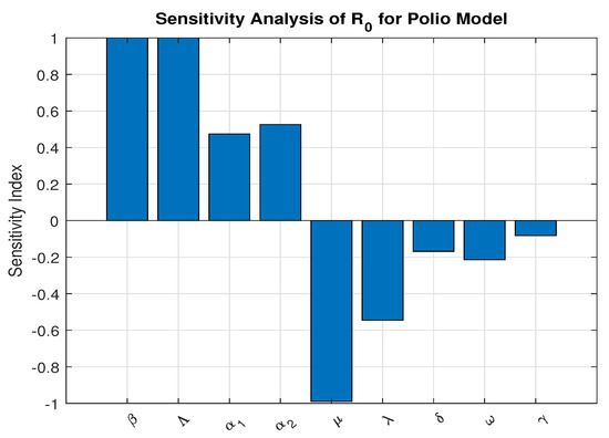
Figure 3. Sensitivity Analysis using parameters values $\mu =0.5,\Lambda =1000,\beta =0.002,{\alpha }_1=0.2,$${\alpha }_2=0.15,\lambda =0.6,\delta =0.9,\omega =0.6,\gamma =0.23.$

The partial derivatives of $R_0$ with respect to each parameter were calculated using the sensitivity index formula:

$${\Gamma }_p^{R_0}={\displaystyle \frac{\partial R_0}{\partial p}}\times {\displaystyle \frac{p}{R_0}}$$

1.

Sensitivity of $\beta$:

$${\displaystyle \frac{\partial R_0}{\partial \beta }}\times {\displaystyle \frac{\beta }{R_0}}=1$$

2.

Sensitivity of $\Lambda$:

$${\displaystyle \frac{\partial R_0}{\partial \Lambda }}\times {\displaystyle \frac{\Lambda }{R_0}}=1$$

3.

Sensitivity of ${\alpha }_1$:

$${\displaystyle \frac{\partial R_0}{\partial {\alpha }_1}}\times {\displaystyle \frac{{\alpha }_1}{R_0}}={\displaystyle \frac{\beta \Lambda \delta }{(\mu +\lambda )(\mu +\delta )(\mu +\omega +\gamma )}}\times {\displaystyle \frac{{\alpha }_1}{R_0}}\approx 0.4743$$

4.

Sensitivity of ${\alpha }_2$:

$${\displaystyle \frac{\partial R_0}{\partial {\alpha }_2}}\times {\displaystyle \frac{{\alpha }_2}{R_0}}={\displaystyle \frac{\beta \Lambda (\mu +\omega +\gamma )}{(\mu +\lambda )(\mu +\delta )(\mu +\omega +\gamma )}}\times {\displaystyle \frac{{\alpha }_2}{R_0}}\approx 0.5257$$

5.

Sensitivity of $\lambda$:

$${\displaystyle \frac{\partial R_0}{\partial \lambda }}\times {\displaystyle \frac{\lambda }{R_0}}\approx -0.5455$$

6.

Sensitivity of $\delta$:

$${\displaystyle \frac{\partial R_0}{\partial \delta }}\times {\displaystyle \frac{\delta }{R_0}}\approx -0.1685$$

7.

Sensitivity of $\mu$:

$${\displaystyle \frac{\partial R_0}{\partial \mu }}\times {\displaystyle \frac{\mu }{R_0}}\approx -0.99$$

8.

Sensitivity of $\omega$:

$${\displaystyle \frac{\partial R_0}{\partial \omega }}\times {\displaystyle \frac{\omega }{R_0}}\approx -0.2140$$

9.

Sensitivity of $\gamma$:

$${\displaystyle \frac{\partial R_0}{\partial \gamma }}\times {\displaystyle \frac{\gamma }{R_0}}\approx -0.0820$$

3.8. Global Sensitivity Analysis

To assess the impact of parameter uncertainty on the basic reproduction number $R_0$, a global sensitivity analysis was performed using the Partial Rank Correlation Coefficient (PRCC) method combined with Latin Hypercube Sampling (LHS). Unlike local sensitivity analysis, which evaluates parameter influence at a single baseline point, global sensitivity analysis accounts for simultaneous parameter variation across biologically feasible ranges, thereby providing a more comprehensive measure of uncertainty.

A total of 10,000 samples were generated using LHS to ensure efficient and uniform exploration of the multidimensional parameter space. For each sampled parameter set, the basic reproduction number $R_0$ was computed. The PRCC values were then calculated to determine the strength and direction of the monotonic relationship between each parameter and $R_0$, while controlling for the effects of other parameters. The parameter ranges and corresponding PRCC results are presented in Table 3 which is graphically presented in Figure 4.

Table 3. Parameter ranges and PRCC results for the basic reproduction number $R_0$.

Parameter	Range	PRCC Value	p-Value
$\beta$	$[0.001,0.003]$	0.7706	0.0000
$\Lambda$	$[500,1500]$	0.7711	0.0000
${\alpha }_1$	$[0.01,0.39]$	0.5794	0.0000
${\alpha }_2$	$[0.01,0.29]$	0.8889	0.0000
$\delta$	$[0.02,0.16]$	−0.5636	0.0000
$\mu$	$[0.01,0.09]$	−0.8726	0.0000
$\lambda$	$[0.02,0.10]$	−0.6715	0.0000
$\omega$	$[0.02,0.10]$	−0.1000	0.0000
$\gamma$	$[0.06,0.40]$	−0.3537	0.0000

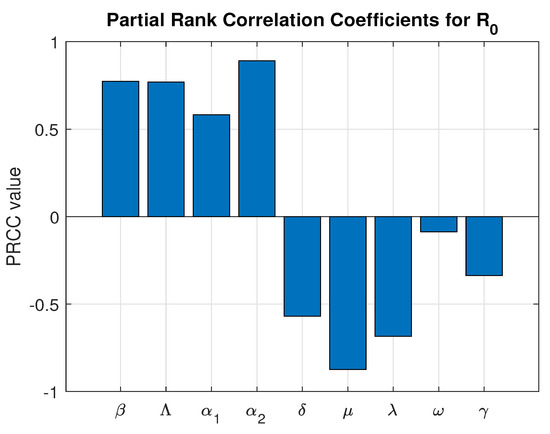
Figure 4. Global Sensitivity Analysis.

The PRCC results indicate that the progression parameter ${\alpha }_2$ and the transmission rate $\beta$ exert the strongest positive influence on $R_0$, confirming that increased transmission intensity and faster progression significantly enhance disease spread.

Notably, the vaccination rate $\lambda$ exhibits a strong and statistically significant negative correlation with $R_0$ (PRCC = −0.6715, p-value $<0.05$). This demonstrates that increasing vaccination coverage substantially reduces the transmission potential of the disease. Among the controllable intervention parameters, $\lambda$ represents one of the most influential mechanisms for driving $R_0$ below the epidemic threshold.

Although the natural mortality rate $\mu$ shows the strongest overall negative correlation, it does not represent a feasible control strategy. In contrast, vaccination is a practical and implementable public health intervention. Therefore, the global sensitivity analysis quantitatively confirms that strengthening immunization programs is a highly effective strategy for disease mitigation and long-term epidemic control.

All parameters are statistically significant, indicating the robustness of the model predictions and reinforcing the reliability of the uncertainty quantification framework.

3.9. Numerical Simulation

3.9.1. Endemic Behavior When $R_0>1$

The analytical results obtained from working on the model’s numerical simulation using the MATLAB ode45 solver are discussed in this section.

We obtain

$$R_0=3.0$$

by selecting the specific values of parameters $\Lambda =60$, $\mu =0.06$, $\beta =0.033$, ${\alpha }_1=0.15$, ${\alpha }_2=0.1$, $\delta =0.93$, $\gamma =0.98$, $\lambda =0.09$, and $\omega =0.01$. Using the initial values $S\left(0\right)=500,I_p\left(0\right)=450,I\left(0\right)=300,V\left(0\right)=150$, and $R\left(0\right)=100$, the graph below is produced. This demonstrates that the population’s infection rate increases with time when $R_0>1$.

In the long term, all the populations of susceptible (S), pre-infectious ($I_p$), infected (I), and Vaccinated (V) decline rapidly. There was a sudden decrease in the number of susceptible populations, indicating a mass outbreak. At the peak of the pandemic, the number of individuals vulnerable to getting the disease declined sharply to a new low.

The recovered (R) population demonstrates a smooth and considerable rise throughout the simulation. This is a direct result of the extensive infection, as much of the population moves from being susceptible, exposed, or infected to being recovered which is graphically presented in Figure 5.

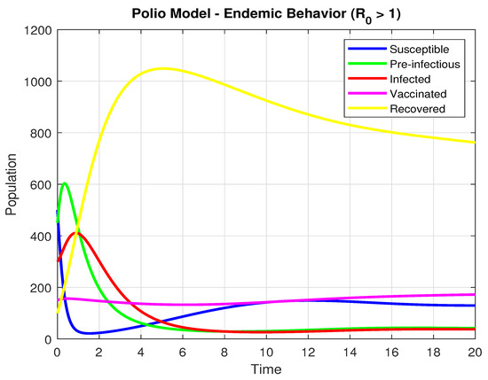
Figure 5. The Population dynamics when $R_0=3.0>1$.

3.9.2. Disease Free Behavior When $R_0<1$

By selecting the particular values of $\Lambda =100$, $\mu =0.059$, $\beta =0.001$, ${\alpha }_1=0.001$, ${\alpha }_2=0.001$, $\delta =0.09$, $\gamma =0.012$, $\lambda =0.004$, $\omega =0.05$. we arrive at

$$R_0=0.0185.$$

Additionally, the starting values are $S\left(0\right)=500,I_p\left(0\right)=450,I\left(0\right)=300,V\left(0\right)=150$, and $R\left(0\right)=100$.

Using the settings mentioned above, the graph below is produced. The graph below is produced. It indicates that the infection is approaching zero when $R_0<1$ and the dynamics are showing in Figure 6.

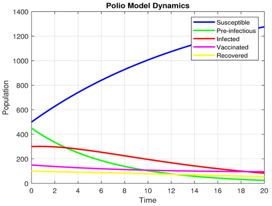
Figure 6. The population dynamics when $R_0=0.0185<1$.

At long last, the pre-infectious ($I_p$), infected (I)and Vaccinated (V) populations all trend strongly downwards to near zero. This means that the disease is not self-maintaining. The number of susceptible (S) individuals, on the other hand, has a uniform rise over time. This is a direct result of the disease disappearing, as fewer people are transitioning to the exposed or infected states. The system’s overall dynamics, whereby the infection disappears and the number of susceptibles increases, is exactly what one should expect when the reproductive number is less than one $R_0<1$.

3.9.3. Effect of Vaccination on Subpopulations

It follows from the Figure 7 that the vaccination rate $\lambda$ significantly affects the dynamics of all subpopulations. For larger values of $\lambda$, the susceptible population $S\left(t\right)$ decreases more rapidly, as there is a quicker movement of individuals into the vaccinated class. Thus, for larger values of $\lambda$, the vaccinated population $V\left(t\right)$ increases more rapidly and settles at a higher equilibrium value. Larger vaccination rates also cause a significant decline in both pre-infectious ($I_p$) and infected $I\left(t\right)$ populations, which decrease more rapidly and reach zero much faster than in the case of small vaccination rates. This is pre-infectious ($I_p$) because increased vaccination reduces the pool of susceptible individuals that are available for infection. Lastly, the recovered population $R\left(t\right)$ is seen to have a decreasing trend for increasing values of $\lambda$ due to the fact that fewer infected individuals result in fewer recoveries. In general, the results show that increased vaccination rates suppress the transmission of the disease, reduce the populations of pre-infectious and infected, and improve long-term protection due to a larger vaccinated population.

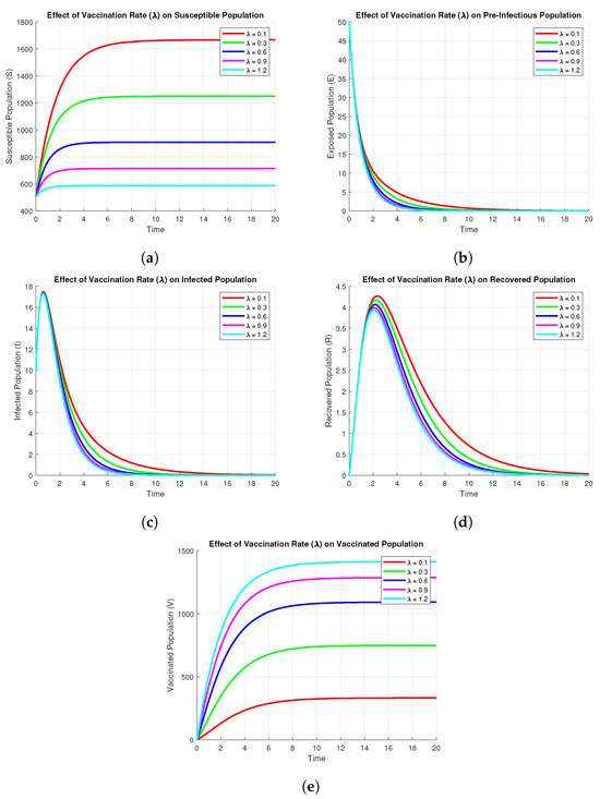
Figure 7. Effect of Vaccination on subpopulations using parameters values $\mu =0.5$, $\Lambda =1000$, $\beta =0.002$, ${\alpha }_1=0.2$, ${\alpha }_2=0.15$, $\delta =0.9$, $\omega =0.6$, $\gamma =0.23$.

3.9.4. Effect of Parameters on Infected

The Figure 8 shows the sensitivity of the infected compartment $I\left(t\right)$, to variations in key model parameters, namely, ${\alpha }_1$, ${\alpha }_2$, $\gamma$, and $\lambda$. From panels $\left(a\right)$ and $\left(b\right)$, one can see that an increase in either ${\alpha }_1$ or ${\alpha }_2$ leads to a higher peak and larger endemic level of infection. In contrast, panels $\left(c\right)$ and $\left(d\right)$ indicate that an increase in $\gamma$ or $\lambda$ decreases both peak and steady-state values of infected individuals, suggesting these parameters are control measures such as recovery or vaccination rates. In general, the analysis identifies those parameters whose change most impacts the dynamics of infection and therefore may offer potential points of intervention.

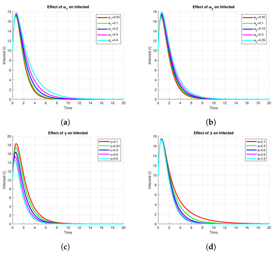
Figure 8. Effect of ${\alpha }_1,{\alpha }_2,\gamma ,\lambda$ on Infected using parameters values $\mu =0.5$, $\Lambda =1000$, $\beta =0.002$, $\delta =0.9$, $\omega =0.6$, ${\alpha }_1=0.2$, ${\alpha }_2=0.15$, $\lambda =0.6$, $\gamma =0.23$.

4. Neural Networking

The methodology of a neural network is like an artificial network that works through hidden layers with the maximum and minimum operations of multiplication and addition using the matrix vectors rules of linear algebra, probability, and data science. The already saved data of the model parameters are putted in the code of NN in matlab package which tested all the data for validation, training, performance, histogram, fitting values and root mean square error (RMSE), mean square error (MSE) and absolute error (AE). The code has the ability to search the data using their built-in function for all such properties given in the figures below. The flow chart for NN is given in Figure 9.

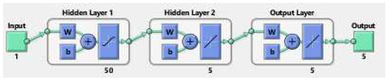
Figure 9. The Neural Network flowchart for target and output values.

For the biological justification, Neural network is linked with numerical simulation of both local stability $R_0<1$ and global stability $R_0>1$ in the form of saved data 1 and data 2 in mathlab 2020 software as usual. After that, the data are used in the neural network code of the MATLAB package in which the target and output built-in functions are already stored in form of hidden layers for the five compartments up to 1000 epochs. The performance and correlations of the data are then tested and worked on with the saved data to train, test, and validate all data along with comparison, regression, absolute error, and mean square error for the already saved data. Further, we extended the discussion of the neural network section. The NN analysis, like AI is the combination of Already saved work related to the said model or its modified versions applied to this model to check its comparison or correlation with the saved numerical simulation in the form of a system of differential equations. This analysis pointed out that the previous works on polio infection are comparable with this model. Furthermore, it has small absolute and mean square errors as the curves of the NN overlap on the previous simulation curves. The NN are performed twice, applied to the saved simulation of the model for $R_0<1$ and $R_0>1$.

Keeping in view the above points, this section presents the neural network analysis of the polio model, representing the dynamics of the compartments based on simulated data for the cases $R_0>1$ and $R_0<1$. The neural network has two or three hidden layers that process the simulated data and return the output in the form of graphs showing all the training, validation, and testing data, along with mean squared errors, performance metrics, regression plots, and fit values. The graphs are shown in Figure 10a–f and Figure 11a–d. Figure 10e is the comparison between the $S{I}_{p}IVR$ model and neural network dynamics for $R_0>1$ while Figure 10f is the absolute error. Similarly, the graphs are shown in Figure 12a–f and Figure 13a–d are neural network dynamics for $R_0<1$. Figure 12e is the comparison of the polio model and neural network dynamics for $R_0<1$, while Figure 12f is the absolute error. Figure 13a–d showing the sample NN along with different characteristics of the model. In both cases, the NN curves are on the curves of human polio dynamics, showing very small mean square errors, which implies the correctness of obtained scheme.

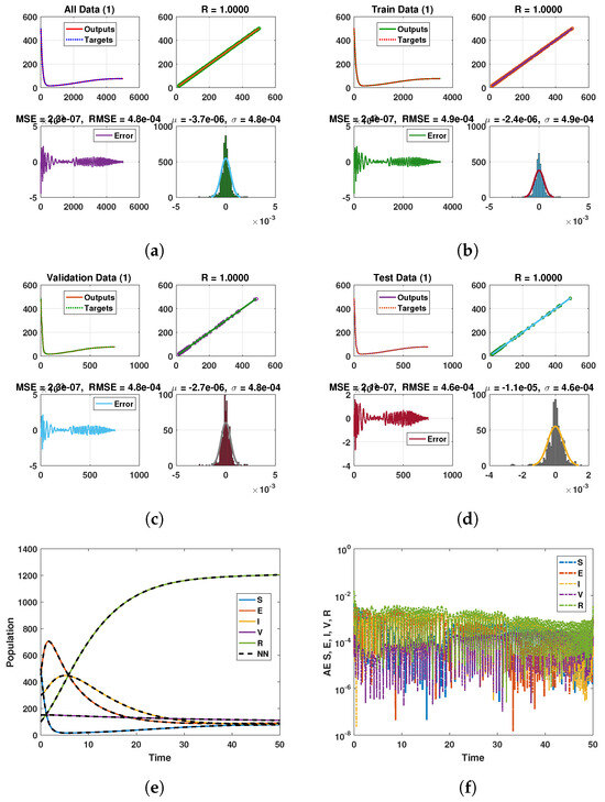
Figure 10. Neural Network dynamics of all five Compartments of Human $S{I}_{p}IVR$ Polio model having $R_0>1$ for (a) All data, (b) Train data, (c) Valid data, (d) Test data, (e) Comparison of Approximate solution with NN and (f) Absolute error.

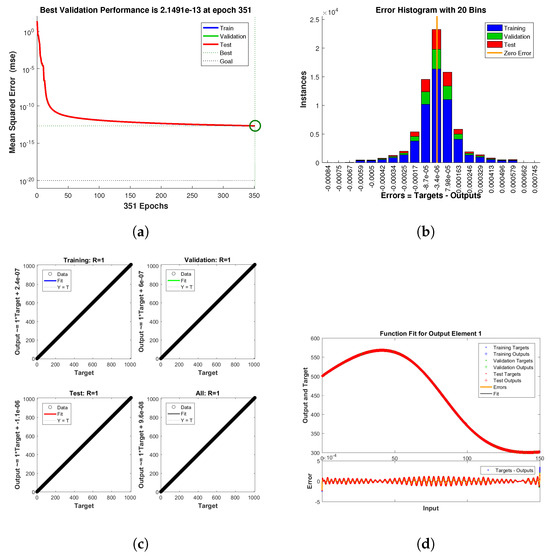
Figure 11. Neural Network dynamics of all five Compartments of Human $S{I}_{p}IVR$ Polio model having $R_0>1$ for (a) Performance, (b) Histogram with error, (c) Regression and (d) Fitting values with error.

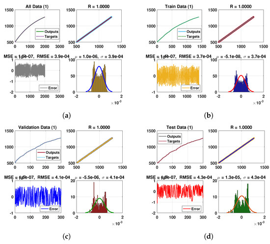
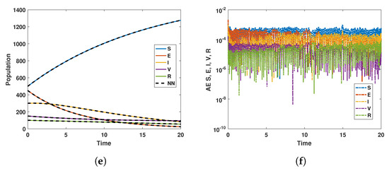
Figure 12. Neural Network dynamics of all five Compartments of Human $S{I}_{p}IVR$ Polio model having $R_0<1$ for (a) All data, (b) Train data, (c) Valid data, (d) Test data, (e) Comparison of Approximate solution with NN and (f) Absolute error.

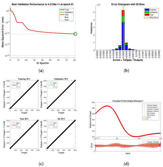
Figure 13. Neural Network dynamics of all five Compartments of Human $S{I}_{p}IVR$ Polio model having $R_0>1$ for (a) Performance, (b) Histogram with error, (c) Regression and (d) Fitting values with error.

5. Conclusions

In this work, a revised $S{I}_{p}IVR$ mathematical model was developed and analyzed to explore the transmission dynamics of poliovirus and the influence of vaccination on disease control. By including a recovered class and an improved force of infection that depends on both pre-infectious and infected individuals, the model captures important epidemiological features that are absent in classical formulations.

We established some basic qualitative properties of the model: positivity, boundedness, and the existence of a biologically feasible invariant region. The basic reproduction number $R_0$ was calculated using the Next Generation Matrix method and we proved its threshold role concerning disease persistence. Our analysis has shown that the disease-free equilibrium is locally and globally asymptotically stable whenever $R_0<1$, and thus the virus is eliminated. When $R_0>1$, there exists a unique endemic equilibrium, and from stability analysis, it follows that infection persists.

Using the central manifold theory and Chavez and Song’s method, we established and analyzed the forward bifurcation. Further, sensitivity analysis identified the most sensitive parameters that greatly affect $R_0$, and recovery rate and vaccination rate played the most critical roles. The results make vaccination a very effective way to reduce infection levels and suppress it for a longer period of time.

Numerical simulations supported the results of the analytical derivations, showing how changes epidemiological parameters alter the dynamics of susceptible, pre-infectious, infected, vaccinated, and recovered populations. The results, in particular, showed that increasing the rate of vaccination substantially suppresses infection, thereby reducing the burden of disease across the population. All the data are tested for the neural network, showing a very small error, which implies the validity of obtained scheme.

Overall, the findings underline that sustaining high vaccination coverage is not only beneficial but essential for achieving eradication and long-term disease control.

5.1. Limitations

It is recognized that numerical simulations within this study are based on parameter values from current literature and reasonable estimations, rather than being calibrated with a specific geographic region or outbreak dataset. Therefore, this limitation does not detract from the theoretical contributions of this work but rather provides a foundation for subsequent applications in specific contexts.

5.2. Future Research Directions

Building on this work, several future directions emerge.

• Model extensions:

Future models should incorporate waning immunity by including transition terms from recovered back to susceptible compartments. They should also differentiate between natural and vaccine-induced immunity for populations with mixed immunity profiles. Additional extensions include booster vaccination, age-structure, spatial dynamics, and environmental transmission.

Future models should incorporate waning immunity, booster vaccination, age structure, spatial dynamics, and environmental transmission.

• Data integration:

The model should be calibrated to real polio data from endemic regions using Bayesian estimation methods.

• Control optimization:

Optimal control theory can design time-varying vaccination strategies, while cost-effectiveness analysis can compare pulse versus continuous vaccination.

• Neural network applications:

Physics-informed neural networks and neural ODEs offer promising tools for parameter identification and data-driven modeling.

These extensions will enhance the model’s applicability for polio eradication efforts.

References

- Nathanson, N. The pathogenesis of poliomyelitis: What we don’t know. Adv. Virus Res. 2008, 71, 1–50. [Google Scholar]
- David, R. Egyptian medicine and disabilities: From pharaonic to greco-roman egypt. In Disability in Antiquity; Routledge: Abingdon, UK, 2016; pp. 91–105. [Google Scholar]
- Mehndiratta, M.M.; Mehndiratta, P.; Pande, R. Poliomyelitis: Historical facts, epidemiology, and current challenges in eradication. Neurohospitalist 2014, 4, 223–229. [Google Scholar] [CrossRef] [PubMed]
- Montero, D.A.; Vidal, R.M.; Velasco, J.; Carreño, L.J.; Torres, J.P.; Benachi O, M.A.; Tovar-Rosero, Y.Y.; Oñate, A.A.; O’Ryan, M. Two centuries of vaccination: Historical and conceptual approach and future perspectives. Front. Public Health 2024, 11, 1326154. [Google Scholar] [CrossRef] [PubMed]
- Aylward, B.; Tangermann, R. The global polio eradication initiative: Lessons learned and prospects for success. Vaccine 2011, 29, D80–D85. [Google Scholar] [CrossRef] [PubMed]
- Mbaeyi, C. Polio vaccination activities in conflict-affected areas. Hum. Vaccines Immunother. 2023, 19, 2237390. [Google Scholar] [CrossRef]
- Kew, O.M.; Wright, P.F.; Agol, V.I.; Delpeyroux, F.; Shimizu, H.; Nathanson, N.; Pallansch, M.A. Circulating vaccine-derived polioviruses: Current state of knowledge. Bull. World Health Organ. 2004, 82, 16–23. [Google Scholar]
- Martinez-Bakker, M.; King, A.A.; Rohani, P. Unraveling the transmission ecology of polio. PLoS Biol. 2015, 13, e1002172. [Google Scholar] [CrossRef]
- Mach, O.; Verma, H.; Khandait, D.W.; Sutter, R.W.; O’Connor, P.M.; Pallansch, M.A.; Cochi, S.L.; Linkins, R.W.; Chu, S.Y.; Wolff, C.; et al. Prevalence of asymptomatic poliovirus infection in older children and adults in northern india: Analysis of contact and enhanced community surveillance, 2009. J. Infect. Dis. 2014, 210, S252–S258. [Google Scholar] [CrossRef]
- Grassly, N.C.; Jafari, H.; Bahl, S.; Durrani, S.; Wenger, J.; Sutter, R.W.; Aylward, R.B. Asymptomatic wild-type poliovirus infection in india among children with previous oral poliovirus vaccination. J. Infect. Dis. 2010, 201, 1535–1543. [Google Scholar] [CrossRef]
- Mohanty, A.; Rohilla, R.; Zaman, K.; Hada, V.; Dhakal, S.; Shah, A.; Padhi, B.K.; Al-Qaim, Z.H.; Altawfiq, K.J.A.; Tirupathi, R.; et al. Vaccine derived poliovirus (vdpv). Infez. Med. 2023, 31, 174. [Google Scholar]
- Liu, X.; Rahman, M.U.; Arfan, M.; Tchier, F.; Ahmad, S.; Mustafa Inc.; Akinyemi, L. Fractional mathematical modeling to the spread of polio with the role of vaccination under non-singular kernel. Fractals 2022, 30, 2240144. [Google Scholar] [CrossRef]
- Thompson, K.M.; Kalkowska, D.A. Review of poliovirus modeling performed from 2000 to 2019 to support global polio eradication. Expert Rev. Vaccines 2020, 19, 661–686. [Google Scholar] [CrossRef] [PubMed]
- Aron, J.L. Mathematical modeling: The dynamics of infection. In Infectious Disease Epidemiology: Theory and Practice; Aspen Publishers: Gaithersburg, MD, USA, 2007; pp. 181–212. [Google Scholar]
- Tolles, J.; Luong, T. Modeling epidemics with compartmental models. JAMA 2020, 323, 2515–2516. [Google Scholar] [CrossRef] [PubMed]
- Biswas, M.H.A.; Paiva, L.T.; de Pinho, M.D.R. A seir model for control of infectious diseases with constraints. Math. Biosci. Eng. 2014, 11, 761–784. [Google Scholar] [CrossRef]
- Grassly, N.C.; Fraser, C. Mathematical models of infectious disease transmission. Nat. Rev. Microbiol. 2008, 6, 477–487. [Google Scholar] [CrossRef]
- Siettos, C.I.; Russo, L. Mathematical modeling of infectious disease dynamics. Virulence 2013, 4, 295–306. [Google Scholar] [CrossRef]
- Dietz, K. The estimation of the basic reproduction number for infectious diseases. Stat. Methods Med. Res. 1993, 2, 23–41. [Google Scholar] [CrossRef]
- Holme, P.; Masuda, N. The basic reproduction number as a predictor for epidemic outbreaks in temporal networks. PLoS ONE 2015, 10, e0120567. [Google Scholar] [CrossRef]
- Gothefors, L. The impact of vaccines in low-and high-income countries. Ann. Nestlé (Engl. Ed.) 2008, 66, 55–69. [Google Scholar] [CrossRef]
- Zhu, X.; Xia, P.; He, Q.; Ni, Z.; Ni, L. Coke price prediction approach based on dense gru and opposition-based learning salp swarm algorithm. Int. J. Bio-Inspired Comput. 2023, 21, 106–121. [Google Scholar] [CrossRef]
- Zhang, X.; Yang, X.; He, Q. Multi-scale systemic risk and spillover networks of commodity markets in the bullish and bearish regimes. N. Am. J. Econ. Financ. 2022, 62, 101766. [Google Scholar] [CrossRef]
- Du, W.; He, Q.; Cao, T.; Wu, J. Intellectual property protection and platform digitalization empowering technology entrepreneurship in emerging markets. Oper. Res. Lett. 2025, 63, 107367. [Google Scholar] [CrossRef]
- Li, B.; Liang, H.; He, Q. Multiple and generic bifurcation analysis of a discrete hindmarsh-rose model. Chaos Solitons Fractals 2021, 146, 110856. [Google Scholar] [CrossRef]
- Eskandari, Z.; Avazzadeh, Z.; Ghaziani, R.K.; Li, B. Dynamics and bifurcations of a discrete-time lotka–volterra model using nonstandard finite difference discretization method. Math. Methods Appl. Sci. 2025, 48, 7197–7212. [Google Scholar] [CrossRef]
- Boden, L.A.; McKendrick, I.J. Model-based policymaking: A framework to promote ethical “good practice” in mathematical modeling for public health policymaking. Front. Public Health 2017, 5, 68. [Google Scholar] [CrossRef] [PubMed]
- Dinleyici, E.C.; Borrow, R.; Safadi, M.A.P.; van Damme, P.; Munoz, F.M. Vaccines and routine immunization strategies during the COVID-19 pandemic. Hum. Vaccines Immunother. 2021, 17, 400–407. [Google Scholar] [CrossRef]
- Tebbens, R.J.D.; Pallansch, M.A.; Chumakov, K.M.; Halsey, N.A.; Hovi, T.; Minor, P.D.; Modlin, J.F.; Patriarca, P.A.; Sutter, R.W.; Wright, P.F.; et al. Expert review on poliovirus immunity and transmission. Risk Anal. 2013, 33, 544–605. [Google Scholar] [CrossRef]
- Thompson, K.M.; Badizadegan, K. Review of poliovirus transmission and economic modeling to support global polio eradication: 2020–2024. Pathogens 2024, 13, 435. [Google Scholar] [CrossRef]
- Shankar, M.; Hartner, A.-M.; Arnold, C.R.K.; Gayawan, E.; Kang, H.; Kim, J.; Gilani, G.N.; Cori, A.; Fu, H.; Jit, M.; et al. How mathematical modelling can inform outbreak response vaccination. BMC Infect. Dis. 2024, 24, 1371. [Google Scholar] [CrossRef]
- Agarwal, M.; Bhadauria, A.S. Modeling spread of polio with the role of vaccination. Appl. Appl. Math. Int. J. (AAM) 2011, 6, 11. [Google Scholar]
- Chitnis, N.; Cushing, J.M.; Hyman, J.M. Bifurcation analysis of a mathematical model for malaria transmission. SIAM J. Appl. Math. 2006, 67, 24–45. [Google Scholar] [CrossRef]
- Rahmi, N.; Fajri, A.; Anggitamaya, A.; Ekasasmita, W.; Kusnaeni, K.; Husain, H.; Nisardi, M.R. Mathematical analysis of polio prevention through vaccination and sanitation: Incorporating incomplete vaccination and virus carrier vectors. ITM Web Conf. 2025, 75, 02006. [Google Scholar] [CrossRef]
- Carr, J. Applications of Centre Manifold Theory; Springer Science & Business Media: Berlin/Heidelberg, Germany, 2012; Volume 35. [Google Scholar]
- Castillo-Chavez, C.; Song, B. Dynamical models of tuberculosis and their applications. Math. Biosci. Eng. 2004, 1, 361–404. [Google Scholar] [CrossRef]
- Lacitignola, D. On the backward bifurcation of a vaccination model with nonlinear incidence. Nonlinear Anal. Model. Control 2016, 16, 30–46. [Google Scholar]
- Elbaz, I.M.; El-Metwally, H.; Sohaly, M.A. Viral kinetics, stability and sensitivity analysis of the within-host COVID-19 model. Sci. Rep. 2023, 13, 11675. [Google Scholar] [CrossRef]
- Taiwo, O.W. Stability and sensitivity analysis of hiv/aids model with saturated incidence rate. Transpublika Int. Res. Exact Sci. 2025, 4, 68–86. [Google Scholar]
- Agbata, B.C.; Obeng-Denteh, W.; Achenecje, G.O.; Amoah-Mensah, J.; Mensa, F.A.; Ezeafulukwe, A.U.; Kwabi, P.A. Mathematical modeling of poliomyelitis with control measure. Dutse J. Pure Appl. Sci. 2024, 10, 186–201. [Google Scholar] [CrossRef]
Disclaimer/Publisher’s Note: The statements, opinions and data contained in all publications are solely those of the individual author(s) and contributor(s) and not of MDPI and/or the editor(s). MDPI and/or the editor(s) disclaim responsibility for any injury to people or property resulting from any ideas, methods, instructions or products referred to in the content. |
© 2026 by the authors. Licensee MDPI, Basel, Switzerland. This article is an open access article distributed under the terms and conditions of the Creative Commons Attribution (CC BY) license.