Symmetry Breaking in Car-Following Dynamics: Suppressing Traffic Oscillations via Asymmetric Dynamic Delays

Abstract

Accurately describing driver response mechanisms is fundamental to microscopic traffic modeling. Traditional car-following models typically assume a fixed reaction time, implying a temporal symmetry where drivers exhibit identical response characteristics during acceleration and deceleration. To address this limitation, this paper proposes a Delay Adaptive Car-following Model that incorporates an asymmetric dynamic delay function to capture the symmetry breaking in driving behavior. Calibrated using empirical trajectory data from the Next Generation Simulation program, the proposed model demonstrates superior accuracy over the conventional Full Velocity Difference Model by effectively reproducing the realistic phenomenon of sluggish acceleration and agile deceleration. Linear stability analysis and numerical simulations reveal that, unlike fixed symmetric delays which often induce instability, the asymmetric dynamic delay acts as a self-adaptive damper. This mechanism suppresses the amplification of disturbances and prevents the formation of stop-and-go waves. The results confirm that incorporating temporal symmetry breaking into delay mechanisms significantly enhances the robustness of traffic flow against oscillations.

1. Introduction

Car-following behavior is an essential characteristic of microscopic traffic flow, and an in-depth investigation of car-following behavior can help understand the dynamic evolution of microscopic traffic flow comprehensively.

Over the past decades, car-following modeling has evolved significantly and can be broadly categorized into data-driven and theory-driven approaches [1,2,3]. Among theory-driven frameworks, the Optimal Velocity Model (OVM) originally proposed by Bando et al. [4] has served as a paradigmatic foundation due to its concise mathematical structure. While the OVM captures basic instability phenomena, Helbing and Tilch [5] identified unrealistic acceleration behaviors and proposed the Generalized Force Model (GFM). Subsequently, Jiang et al. [6] introduced the Full Velocity Difference Model (FVDM) by incorporating the velocity difference term, which resolved the unrealistic deceleration issues of GFM and significantly improved stability analysis.

Given the robustness of the FVDM framework, numerous extensions have been developed to incorporate complex driving factors. Recent studies have investigated the impacts of varying spacing headway [7], electronic throttle control [8], acceleration memory [9], connected environment information [10], and heterogeneous traffic characteristics [11,12,13,14]. These studies have enriched our understanding of car following behavior under specific conditions. However, the temporal symmetry of driver reaction mechanisms remains a key issue and has been oversimplified in most studies.

Reaction delay is an inherent physiological and mechanical property of driving. Early works by Pipes [15] and Newell [16] established that drivers require a finite time to perceive and process stimuli. While Bando et al. [17] and subsequent researchers [18,19,20,21,22,23] integrated explicit delay terms into the OVM and FVDM frameworks, these models typically treat the reaction time as a constant parameter or a simple linear function of headway. This treatment implies a temporal symmetry hypothesis assuming that drivers exhibit identical response latencies during both acceleration and deceleration phases. However, this assumption contradicts empirical observations in traffic psychology and physics. Real-world driving behavior exhibits significant symmetry breaking, where drivers tend to react sluggishly when accelerating to maintain comfort and fuel economy but demonstrate agile and high-sensitivity responses when decelerating to ensure safety [12].

Neglecting this asymmetry leads to biased estimations of traffic stability. Models with fixed symmetric delays often overestimate instability during acceleration or underestimate safety risks during braking. Although some studies have explored multiple time delays [24,25,26,27,28] or state-dependent behaviors [29,30,31], few have explicitly modeled the symmetry breaking mechanism in delays to explain the suppression of traffic oscillations. Zhu et al. [32] and Kim et al. [33] further noted that total delay comprises not only cognitive reaction time but also vehicle mechanical response time, and both of them vary dynamically with motion states.

To the best of our knowledge, many studies have considered the driver’s reaction delay in the car-following model but setting the reaction delay of the driver as a constant is inconsistent with the real driving behavior. In addition, the varying reaction-time delays can effectively ensure the robust stability of traffic flow and suppress traffic jams. However, the researchers only considered the driver’s reaction delay in their study. Therefore, a car-following model that considers both the driver’s reaction delay and the vehicle’s mechanical response time is proposed in this study, wherein the constant reaction delay in the traditional model is improved to a dynamic delay function. The results of empirical analysis and numerical simulations show that considering the driver–vehicle dynamic delay can improve not only the prediction accuracy of the proposed model but also its linear stability and dynamic performance.

The remainder of this paper is organized as follows. An improved car-following model that considers the driver–vehicle dynamic delay is proposed in Section 2. The proposed model is calibrated and validated using vehicle trajectory data in Section 3. The linear stability analysis is performed in Section 4. Different numerical simulation schemes are carried out to verify the reliability of the proposed model in Section 5. Finally, the study is summarized and conclusions from this study are drawn in Section 6.

2. Methodology

In microscopic traffic flow modeling, accurately describing the driver’s response mechanism to stimuli is crucial. Traditional car-following models typically assume that drivers possess a fixed reaction time for the sake of mathematical simplicity. This treatment implies a temporal symmetry assumption, i.e., considering that the neural and mechanical response characteristics of drivers are identical during acceleration and deceleration processes. However, actual driving behavior often exhibits significant asymmetric characteristics. This section will derive and construct a driver-vehicle dynamic delay model considering asymmetric characteristics based on the symmetric delay assumption of traditional models.

2.1. Symmetric Delay Assumption in Traditional Models

As early as 1961, Newell [16] pointed out that there is a stimulus-response delay for drivers and proposed the car-following model shown in Equation (1).

$$v_n\left(t+\tau \right)=V\left(∆x\left(t\right)\right),$$

(1)

where $v_n$ is the velocity of the following vehicle, $\tau$ is the driver’s reaction delay, and $∆x_n\left(t\right)$ is the spacing headway. In this model, $\tau$ is treated as a constant, meaning the model assumes that vehicle dynamics are translationally symmetric in time. $V\left(∆x_n\left(t\right)\right)$ is the optimal velocity function, expressed as Equation (2).

$$V\left(∆x\left(t\right)\right)=v_{\mathrm{m}\mathrm{a}\mathrm{x}}-v_{\mathrm{m}\mathrm{a}\mathrm{x}}\cdot \mathrm{e}\mathrm{x}\mathrm{p}\left[-{\displaystyle \frac{c}{v_{\mathrm{m}\mathrm{a}\mathrm{x}}}}\cdot \left(∆x\left(t\right)-d_n\right)\right],$$

(2)

where $v_{max}$ is the maximum velocity, $c$ is a parameter, and $d_n$ is the minimum spacing.

Bando et al. [4] subsequently proposed the OVM, assuming that drivers control the pedal to eliminate the deviation between the current velocity and the optimal velocity, as shown in Equation (3).

$$a_n\left(t\right)=k\cdot \left[V\left(∆x\left(t\right)\right)-v_n\left(t\right)\right],$$

(3)

where $k$ is the sensitivity parameter. The optimal velocity function adopted by this model is shown in Equation (4).

$$V\left(∆x\left(t\right)\right)={\displaystyle \frac{v_{\mathrm{m}\mathrm{a}\mathrm{x}}}{2}}\cdot \left[\mathrm{t}\mathrm{a}\mathrm{n}\mathrm{h}\left(∆x\left(t\right)-h_c\right)+\mathrm{t}\mathrm{a}\mathrm{n}\mathrm{h}\left(h_c\right)\right],$$

(4)

where $h_c$ is the safety spacing. Notably, although the OVM does not have an explicit delay term, it implies a response mechanism similar to the Newell model. By expanding the left side of Equation (1) using the Taylor series and ignoring higher-order terms, Equation (5) can be obtained.

$$v_n\left(t+\tau \right)=v_n\left(t\right)+\tau \cdot a_n\left(t\right).$$

(5)

Substituting Equation (5) into Equation (1) and rearranging yields Equation (6).

$$a_n\left(t\right)={\displaystyle \frac{1}{\tau }}\cdot \left[V\left(∆x\left(t\right)\right)-v_n\left(t\right)\right]=k\cdot \left[V\left(∆x\left(t\right)\right)-v_n\left(t\right)\right].$$

(6)

Comparing Equations (3) and (6), it can be seen that the sensitivity parameter $k$ in the OVM is essentially the reciprocal of the driver’s reaction delay $\tau$. Since $k$ is usually set as a constant in the OVM, this further confirms that traditional models imply the assumption that reaction delay remains unchanged (i.e., symmetric) under different driving states.

Jiang et al. [6] introduced the velocity difference term on this basis and proposed the Full Velocity Difference Model (FVDM) to address the limitations of the OVM, as shown in Equation (7).

$${\displaystyle \frac{d{v}_n\left(t\right)}{dt}}=k\cdot \left[V\left(∆x\left(t\right)\right)-v_n\left(t\right)\right]+\lambda \cdot ∆v\left(t\right),$$

(7)

where $∆v_n\left(t\right)$ is the velocity difference. Although the FVDM improves stability, it still inherits the constant $k$ setting, thereby ignoring the asymmetric delay effect prevalent in real driving.

2.2. Improved Model Considering Asymmetric Delay

Zhu et al. [32] pointed out that total delay includes not only the driver’s cognitive reaction time but also the vehicle’s mechanical response time. More importantly, from physics and psychology perspectives, there are essential differences in the driver’s behavioral patterns during acceleration (catching up with the preceding vehicle) and deceleration (collision avoidance), leading to symmetry breaking in time.

To mathematically describe this asymmetry, this study introduces the dynamic delay time function proposed by Ozaki [34]. This function explicitly constructs delay characteristics under two different phase planes, acceleration and deceleration, through a piecewise form, as shown in Equation (8). This function is derived from the empirical regression analysis conducted by Ozaki using real-world data. The constant term represents the inherent baseline delay, while the coefficients of the subsequent terms represent the sensitivity of the delay to changes in spacing headway and acceleration (or deceleration). Specifically, the difference in these coefficients captures the driver’s asymmetric behavior: sluggishness during acceleration and agility during deceleration.

$$T\left(∆x,a_n\right)=\left\{\begin{array}{cc}0.743+0.016·∆x\left(t\right)+0.037·a_n\left(t-∆t\right),& \mathrm{d}\mathrm{e}\mathrm{c}\mathrm{e}\mathrm{l}\mathrm{e}\mathrm{r}\mathrm{a}\mathrm{t}\mathrm{i}\mathrm{o}\mathrm{n}\\ 0.886+0.008·∆x\left(t\right)+0.037·a_n\left(t-∆t\right),& \mathrm{a}\mathrm{c}\mathrm{c}\mathrm{e}\mathrm{l}\mathrm{e}\mathrm{r}\mathrm{a}\mathrm{t}\mathrm{i}\mathrm{o}\mathrm{n}\end{array}\right..$$

(8)

It should be noted here that Equation (8) is discontinuous and non-differentiable at zero acceleration (deceleration). This implies that the delay value exhibits a jump discontinuity when the driver switches between acceleration and deceleration states. However, this jump discontinuity precisely captures the realistic behavioral characteristics of drivers, as the operation of vehicle acceleration and deceleration by drivers is not a smooth transition but a discrete event. Thus, Equation (8) can accurately model the asymmetry of driving behavior. Furthermore, the acceleration (deceleration) during car-following may fluctuate around zero, causing the delay value calculated by Equation (8) to change frequently and become unstable. To avoid this problem, a hysteresis switching mechanism is introduced to control the transition between acceleration and deceleration states, as shown in Equation (9).

$$S\left(t\right)=\left\{\begin{array}{cc}1,& \mathrm{i}\mathrm{f} a_n\left(t-∆t\right)>ϵ\\ -1,& \mathrm{i}\mathrm{f} a_n\left(t-∆t\right)<-ϵ\\ S\left(t-∆t\right),& \mathrm{o}\mathrm{t}\mathrm{h}\mathrm{e}\mathrm{r}\mathrm{w}\mathrm{i}\mathrm{s}\mathrm{e}\end{array}\right..$$

(9)

Specifically, $S\left(t\right)$ represents the current control state, and $S\left(t-∆t\right)$ represents the control state at the previous time step. If $S\left(t\right)=1$, it indicates that the delay term uses acceleration; if $S\left(t\right)=-1$, it indicates that the delay term uses deceleration; if $S\left(t\right)=S\left(t-∆t\right)$, it indicates that the motion state of the previous time step is maintained. $ϵ$ is set to $0.1\times {10}^{-3}$ m/s² to avoid unreasonable driving mode switching caused by noise.

Based on the above analysis, we propose an improved car-following model capable of characterizing asymmetric dynamic features—the Delay Adaptive Car-following Model (DACM). This model replaces the constant delay parameter in traditional models with the asymmetric dynamic delay function $T\left(∆x,a_n\right)$.

Considering the cognitive mechanism during driving, the driver’s judgment of the safe distance ahead is significantly affected by their reaction time and the vehicle’s mechanical lag. In contrast, the driver’s perception of velocity difference is often based on instantaneous visual stimuli, possessing a faster response speed. Existing studies indicate that the change in spacing headway is the dominant factor inducing drivers to adjust speed, while dynamic delay mainly manifests as the lag when the driver adjusts the expected speed [24]. Furthermore, under the FVDM framework, the velocity difference term mainly plays a role in stabilizing traffic flow. To focus on exploring the dominant effect of driver-vehicle asymmetric dynamic delay on car-following behavior and to maintain the physical simplicity of the model, this study explicitly introduces the dynamic delay term into the optimal velocity function while ignoring the relatively minor delay influence in the velocity difference term. The improved dynamics equation is shown in Equation (10).

$${\displaystyle \frac{d{v}_n\left(t\right)}{dt}}=k\cdot \left[V\left(∆x\left(t-T\left(∆x,a_n\right)\right)\right)-v_n\left(t\right)\right]+\lambda \cdot ∆v\left(t\right),$$

(10)

where the optimal velocity function is shown in Equation (11).

$$V\left(∆x\left(t\right)\right)=V_1+V_2\cdot \mathrm{t}\mathrm{a}\mathrm{n}\mathrm{h}\left[C_1\cdot \left(∆x\left(t\right)-l_c\right)-C_2\right],$$

(11)

where $V_1,V_2,C_1,C_2$ are parameters, and $l_c$ is the vehicle length.

By introducing the asymmetric delay term from Equation (8), Equation (10) constructs a nonlinear dynamic system with state-dependent time lag. This improvement enables the model to capture the hysteresis effects ignored by traditional symmetric models, thereby more realistically reproducing the complex evolutionary phenomena in traffic flow.

3. Data and Model Calibration

3.1. Data Description and Processing

This study leverages high-precision vehicle trajectory data from the Next Generation Simulation (NGSIM) program administered by the U.S. Federal Highway Administration [35]. Given the focus of this research on car-following dynamics in continuous traffic flow, trajectory data from the US-101 highway segment in Los Angeles, California, was selected for analysis. Collected during the morning peak period on 15 June 2005, the complete 45 min dataset comprises three 15 min intervals: (1) 7:50 a.m. to 8:05 a.m., (2) 8:05 a.m. to 8:20 a.m., and (3) 8:20 a.m. to 8:35 a.m. Characterized by both congested stop-and-go traffic waves and free-flow conditions, this segment is well-suited for investigating the nonlinear delay properties inherent in car-following behavior [36].

To explicitly investigate car-following interactions, we applied stringent filtering criteria to the raw dataset [37]. First, specific filters were set to minimize heterogeneity: only passenger cars driving on main Lanes 1–5 were retained, excluding trucks and vehicles on auxiliary lanes. Second, a valid car-following pair was defined by strict ID matching—ensuring the Preceding_ID of the follower matched the Vehicle_ID of the leader—and trajectories were synchronized based on Frame_ID to ensure strict temporal alignment. Third, to capture complete oscillation processes, only segments with a continuous duration exceeding 60 s without lane-changing maneuvers were extracted. Based on these rules, 1500 valid car-following pairs were obtained. Finally, to handle measurement noise and outliers, we adopted a physical threshold truncation strategy. Specifically, negative velocities were corrected to 0 m/s, and accelerations and decelerations were restricted within the range of $\left[-3.4, 3.4\right]$ m/s². Additionally, the headway between vehicles was limited to the physical limit range of $\left[5, 80\right]$ m. For each pair, the key attributes extracted for analysis include Vehicle_ID, Frame_ID, Fol_Velocity (v_Vel), Fol_Acceleration (v_Acc), Lane_ID, Preceding_ID, Following_ID, Space_Headway, and Time_Headway.

Given the measurement noise in the raw NGSIM data, direct differentiation would lead to non-physical and violent oscillations in velocity and acceleration. To address this, we employed the Robust Locally Weighted Regression (RLOWESS) method [38,39] to smooth the position data $x\left(t\right)$. Specifically, the smoothing process was implemented using an adaptive window strategy, where the window span was set to 2% of the total data points for each trajectory. This bandwidth was selected to filter out measurement noise while preserving the trajectory’s valid dynamic features. To ensure kinematic consistency, velocity $v\left(t\right)$ and acceleration $a\left(t\right)$ were obtained strictly by first-order and second-order numerical differentiation of the smoothed position data. Furthermore, to address the zero-speed drift phenomenon that may be produced by the regression algorithm when the vehicle is stationary, a zero-speed correction step was introduced: when the raw velocity is below a threshold for a continuous period, the smoothed velocity and acceleration are forced to zero.

The comparison of data before and after processing is shown in Figure 1. It can be observed that the processed trajectories eliminate high-frequency noise while retaining critical dynamic characteristics during acceleration and deceleration processes.

The processed data were divided into two non-overlapping subsets: 70% of the car-following groups were randomly selected for model parameter calibration, and the remaining 30% were used for model validation. This partition method based on vehicle groups rather than data points can effectively improve the calibration accuracy of the model.

3.2. Model Calibration

The objective of model calibration is to find a set of optimal parameters that minimizes the discrepancy between the simulated trajectories and the observed real trajectories. Considering the strong global search capability and robustness of the Genetic Algorithm in solving nonlinear optimization problems [40], this study employs an improved genetic algorithm to estimate the model parameters.

According to the study by Kesting et al. [41], the cumulative effect of errors is most sensitive to spacing headway. Therefore, we selected the Root Mean Square Normalized Error (RMSNE) of the spacing headway as the objective function [42], as shown in Equation (12).

$$\mathrm{R}\mathrm{M}\mathrm{S}\mathrm{N}\mathrm{E}=\sqrt{{\displaystyle \frac{1}{N}}\sum _{i=1}^N{\left({\displaystyle \frac{P_i-O_i}{O_i}}\right)}^2},$$

(12)

where $P_i$ and $O_i$ are the predicted and observed values of spacing headway, respectively, and $N$ is the total number of samples.

We initialized the model parameters on the basis of the empirical findings reported by Yu et al. [43], followed by parameter calibration via a Genetic Algorithm. The final parameter set was determined by minimizing the RMSNE on the validation set, thereby ensuring the accuracy of the model in reproducing trajectories. In addition, to avoid overfitting caused by excessive degrees of freedom, we directly adopted the empirical regression analysis results from Ozaki [34] for the coefficients in Equation (8). The initial parameters of the genetic algorithm are set as follows: population size, 100; adaptive crossover probability interval, [0.5, 0.9]; scale coefficient, 0.75; mutation probability, 0.1; and maximum number of generations, 300. The range of main parameters for the model is $k\in \left[\mathrm{0,1}\right]$ and $\mathsf{\lambda }\in \left[\mathrm{0,1}\right]$, while others are consistent with those in the literature [6]. A penalty term is added to the fitness function to eliminate the effects of certain parameter combinations that may lead to unreasonable results in the car-following model [42]. Additionally, since the genetic algorithm is a stochastic search algorithm, the optimal solution may vary slightly for each optimization run. Therefore, the solving process is repeated 50 times, and the set of optimal parameters yielding the minimum error is selected. The calibration results are presented in

Table 1. Calibration result of FVDM and DACM.

Parameter	$\mathit{k}$	$\mathit{\lambda }$
FVDM	0.36	0.84
DACM	0.12	0.97

.

Comparing the parameters in Table 1, an interesting phenomenon can be observed: the sensitivity parameter $k$ of the DACM is significantly lower than that of the FVDM. From a physical perspective, the sensitivity parameter in the FVDM not only carries the driver’s reaction intensity to the spacing headway but also implicitly compensates for the neglected delay effects. In contrast, in the DACM, due to the introduction of an explicit dynamic delay term to specifically describe the response lag, the sensitivity parameter reverts to its essence of reflecting pure control gain. This indicates that the DACM more accurately characterizes the driving mechanism by decoupling the delay effect from the control gain.

3.3. Empirical Verification

To verify the generalization ability of the model on unseen data, we evaluated the model from two dimensions: statistical distribution characteristics and prediction accuracy. Based on the validation set data, we compared the acceleration distributions of the observed values and the predicted values of the two models, as shown in Figure 2.

To quantitatively evaluate the prediction accuracy, we adopted the Root Mean Square Error (RMSE) as the evaluation metric, as shown in Equation (13).

$$\mathrm{R}\mathrm{M}\mathrm{S}\mathrm{E}=\sqrt{{\displaystyle \frac{1}{N}}{\sum }_{i=1}^N{\left(P_i^a-O_i^a\right)}^2},$$

(13)

where $P_i^a$ and $O_i^a$ are the predicted and observed values of acceleration, respectively. The statistical results are shown in

Table 2. Validation results (RMSE) of FVDM and DACM.

Model	Average	Median	Min	Max	Std
FVDM	1.61	1.52	0.71	3.34	0.47
DACM	0.92	0.88	0.46	3.21	0.27

.

As shown in Table 2, the average RMSE of the DACM is 0.92, which is reduced by about 42.9% compared to 1.61 of the FVDM. Moreover, the error standard deviation of the DACM is smaller, indicating that its performance is more robust under different car-following scenarios. This significant improvement in accuracy confirms that considering the driver-vehicle dynamic delay (especially its asymmetry during acceleration and deceleration) can greatly correct the deviation of traditional models in describing the complex evolution of traffic flow. Moreover, to analyze whether the asymmetric delay mechanism is superior to the symmetric mechanism under dynamic delay conditions, we theoretically analyzed the error of the symmetric mechanism. We assumed that the dynamic delay of the symmetric mechanism was calculated using the formula under acceleration mode (see Equation (8)), but the constant term was taken as the average value (0.81) under both acceleration and deceleration modes. Since the acceleration and deceleration delays under both the asymmetric and symmetric mechanisms are very close ($∆T=0.14$ s), the RMSE difference is not significant under the same parameter configuration. Therefore, in subsequent circular road simulations, we focused on exploring the differences between the asymmetric and symmetric mechanisms in suppressing traffic oscillations, compensating for the limitations of relying solely on fitting error to evaluate model performance.

4. Linear Stability Analysis

In this section, the linear stability theory is used to analyze the stability of the car-following model. For steady-state traffic flow, it can be described by Equation (14).

$$\left\{\begin{array}{l}{x}_n^0\left(t\right)=b·n+V\left(b\right)·t\\ ∆x_n^0\left(t\right)=b\\ v_n^0\left(t\right)=V\left(b\right)\end{array}\right.,$$

(14)

where $x_n^0\left(t\right)$ is the initial position of the $n$-th vehicle, $b$ is the spacing headway under steady-state traffic flow, $∆x_n^0\left(t\right)$ is the initial spacing headway of the $n$-th vehicle, and $v_n^0\left(t\right)$ is the initial velocity of the $n$-th vehicle.

Applying an initial small perturbation to the $n$-th vehicle in the car-following platoon, denoted by $y_n\left(t\right)$, the position of the $n$-th vehicle can be rewritten as Equation (15).

$$x_n\left(t\right)=x_n^0\left(t\right)+y_n\left(t\right).$$

(15)

According to Equations (14) and (15), the following results can be obtained as shown in Equation (16).

$$\left\{\begin{array}{l}{\dot{x}}_n\left(t\right)=V\left(b\right)+{\dot{y}}_n\left(t\right)\\ {\ddot{x}}_n\left(t\right)={\ddot{y}}_n\left(t\right)\\ ∆x\left(t\right)=b+∆y_n\left(t\right)\end{array}\right..$$

(16)

It should be specifically noted that the linear stability analysis examines the local properties of the system under infinitesimal perturbations. Therefore, we adopt a first-order approximation valid near the equilibrium state, treating the dynamic delay function $T\left(∆x,a_n\right)$ as a constant value determined solely by the steady-state headway $b$ (since acceleration is zero at equilibrium). This approximation effectively reduces the governing equation to a constant-delay differential equation in the vicinity of the equilibrium point. At steady state, the acceleration is zero; according to Equation (8), the dynamic delay is determined solely by the steady-state spacing. Based on this assumption, substituting Equation (16) into Equation (10), the following equation regarding the disturbance can be obtained as Equation (17).

$${\ddot{y}}_n\left(t\right)=k\cdot \left[V\left(b+∆y_n\left(t\right)-{\dot{y}}_{n-1}\left(t\right)\cdot T\left(∆x,a_n\right)+{\dot{y}}_n\left(t\right)\cdot T\left(∆x,a_n\right)\right)-V\left(b\right)-{\dot{y}}_n\left(t\right)\right]+\lambda \cdot ∆{\dot{y}}_n\left(t\right).$$

(17)

Expanding the optimal velocity function in Equation (17) by using the Taylor series, we can get Equation (18).

$$V\left(b+∆y_n\left(t\right)-{\dot{y}}_{n-1}\left(t\right)\cdot T\left(∆x,a_n\right)+{\dot{y}}_n\left(t\right)\cdot T\left(∆x,a_n\right)\right)=V\left(b\right)+V^{\prime }\left(b\right)\cdot \left[∆y_n\left(t\right)-{\dot{y}}_{n-1}\left(t\right)\cdot T\left(∆x,a_n\right)+{\dot{y}}_n\left(t\right)\cdot T\left(∆x,a_n\right)\right].$$

(18)

Thus, Equation (17) can be rewritten as Equation (19).

$${\ddot{y}}_n\left(t\right)=k\cdot \left[V^{\prime }\left(b\right)\cdot ∆y_n\left(t\right)-V^{\prime }\left(b\right)\cdot ∆{\dot{y}}_n\left(t\right)\cdot T\left(∆x,a_n\right)-{\dot{y}}_n\left(t\right)\right]+\lambda \cdot ∆{\dot{y}}_n\left(t\right).$$

(19)

Let $y_n\left(t\right)=e^{i\mathsf{\omega }n+zt}$ and substitute it into Equation (19), the following results are obtained as shown in Equation (20).

$$z^2+z\cdot \left[k\cdot V^{\prime }\left(b\right)\cdot T\left(∆x,a_n\right)\cdot \left(e^{-i\omega }-1\right)+k-\lambda \cdot \left(e^{-i\omega }-1\right)\right]-k\cdot V^{\prime }\left(b\right)\cdot \left(e^{-i\omega }-1\right)=0.$$

(20)

Then, let $e^{-i\mathsf{\omega }}-1\approx -i\mathsf{\omega }+{\displaystyle \frac{{\left(i\mathsf{\omega }\right)}^2}{2}}$ and $z\approx z_1\left(i\mathsf{\omega }\right)+z_2{\left(i\mathsf{\omega }\right)}^2$. Equation (20) can be rewritten as an equation with respect to $z_1$ and $z_2$ as shown in Equation (21).

$${z_1}^2{\left(i\omega \right)}^2-z_1{\left(i\omega \right)}^2\cdot k\cdot V^{\prime }\left(b\right)\cdot T\left(∆x,a_n\right)+z_1\left(i\omega \right)\cdot k+z_2{\left(i\omega \right)}^2\cdot k+z_1{\left(i\omega \right)}^2\cdot \lambda -k\cdot V^{\prime }\left(b\right)\cdot \left({\displaystyle \frac{1}{2}}{\cdot \left(i\omega \right)}^2-i\omega \right)=0.$$

(21)

The first-order term and second-order term with respect to $i\mathsf{\omega }$ are given in Equation (22), respectively.

$$\left\{\begin{array}{l}{z}_1={-V}^{\prime }\left(b\right)\\ z_2={\displaystyle \frac{V^{\prime }\left(b\right)\cdot \left(\lambda +\frac{k}{2}\right)-{V^{\prime }\left(b\right)}^2\cdot \left(1+k\cdot T\left(∆x,a_n\right)\right)}{k}}\end{array}\right..$$

(22)

Thus, the neutral stability condition of the proposed model is given in Equation (23).

$$V^{\prime }\left(b\right)={\displaystyle \frac{2·\lambda +k}{2+2·k\cdot T\left(∆x,a_n\right)}}.$$

(23)

It can be seen from Equation (23) that when $T=0$, the neutral stability condition of the DACM is consistent with the FVDM; when $T=0$ and $\mathsf{\lambda }=0$, the neutral stability condition of the DACM is consistent with the OVM. Furthermore, according to the long-wave theory, the stability domain of uniform flow can be expressed as Equation (24).

$$T\left(∆x,a_n\right)<{\displaystyle \frac{2·\lambda +k-{2·V}^{\prime }\left(b\right)}{{2·V}^{\prime }\left(b\right)·k}}.$$

(24)

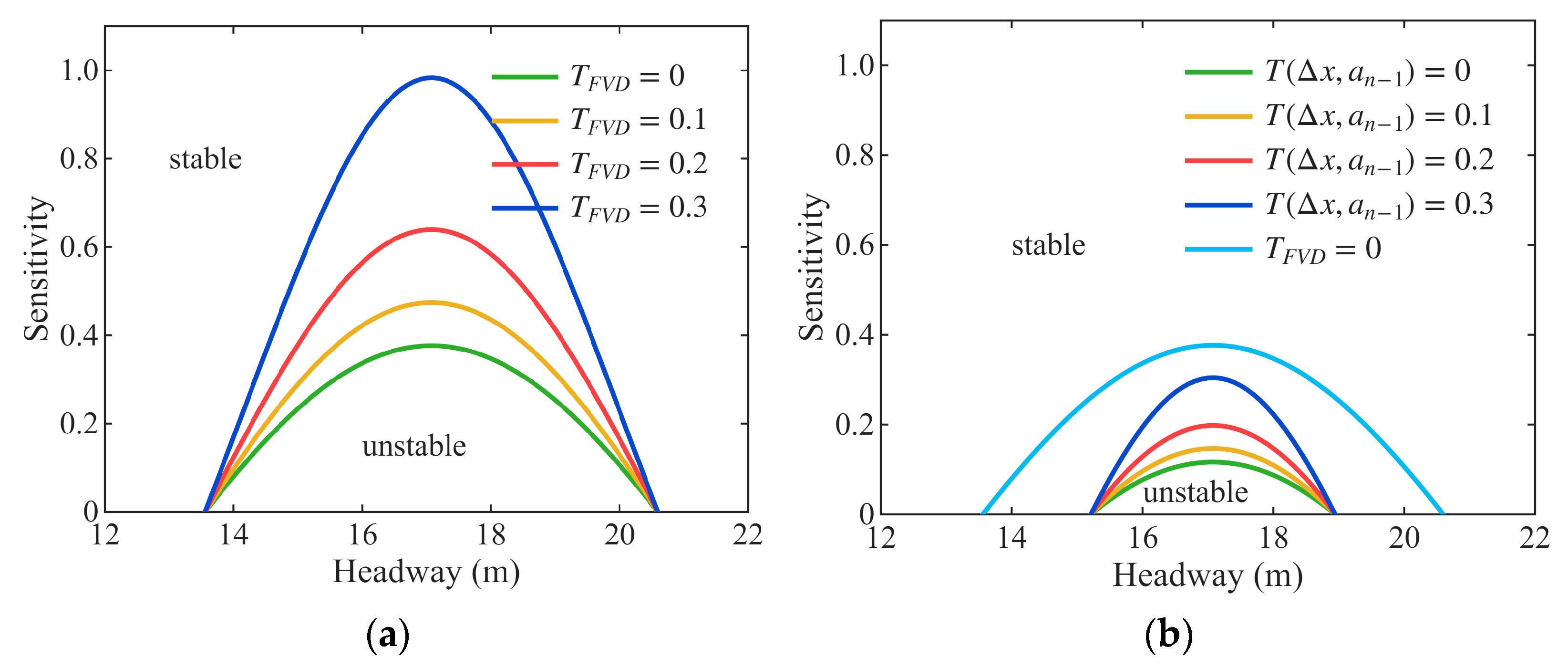
Equation (24) reveals the profound influence of delay time $T$ on traffic flow stability. To intuitively illustrate the difference in stability between the proposed DACM and the traditional FVDM, we plotted the neutral stability curves in the headway-sensitivity space, as shown in Figure 3.

From Figure 3a, it can be seen that for the FVDM, as the artificially introduced fixed delay time increases, the stable region shrinks significantly. This implies that the delay effect is fundamentally a factor that destroys system symmetry and stability. Figure 3b shows the stability performance of the DACM. Notably, although the DACM introduces delay, under the same magnitude of delay (e.g., comparing the case of $T=0.3 \mathrm{s}$), the stable region of the DACM is noticeably larger than that of the FVDM. This improvement is attributed to two key factors: First, the parameter $k$ in the DACM decouples the pure gain regulation function from the delay effect, making the system mathematically more robust. Second, and more importantly, the asymmetric delay mechanism acts as a physical stabilizer. Specifically, the larger delay during acceleration acts as a low-pass filter that dampens high-frequency disturbances, preventing them from growing into traffic oscillations, while the smaller delay during deceleration ensures a rapid response to braking signals. This dual mechanism expands the stable region compared to the fixed-delay model, thereby enhancing the overall robustness of the traffic flow. Figure 3 further indicates that the asymmetric delay mechanism alters the stability boundary without changing the fundamental type of bifurcation. From the perspective of dynamical systems, the traffic flow system still undergoes Hopf bifurcation. However, the introduction of the asymmetric delay mechanism effectively expands the stable region, that is, it shifts the critical stability curve, thereby enhancing the traffic flow system’s ability to resist disturbances.

Although the linear stability analysis is based on the equilibrium state, the dynamic delay in Equation (24) is actually determined by Equation (8). This means that in real nonlinear traffic flow evolution, vehicles will dynamically switch between different stability boundaries according to their asymmetric acceleration or deceleration states. This dynamic adjustment mechanism enables the DACM to dissipate disturbances more effectively than a single fixed-delay model, thereby suppressing the occurrence of traffic congestion. However, given that the dynamic delay function is approximated to the first order near the equilibrium state, the derived stability conditions are first-order approximate criteria applicable in the vicinity of the equilibrium point. This result may not fully capture the complex nonlinear dynamics induced by the time-varying nature of the delay. To address the limitations of linear stability analysis, this study focuses on investigating the oscillation suppression mechanism of the asymmetric delay under nonlinear conditions in the Section 5.

5. Numerical Simulation

This section conducts numerical simulations to comprehensively validate the effectiveness of the proposed model. We first clarify the microscopic mechanism of asymmetric time delay in Section 5.1, thereby establishing a physical foundation for subsequent experiments. To ensure that the simulation can cover typical car-following scenarios, we designed two complementary scenarios. In Section 5.2, we simulated the discrete acceleration and braking processes representing deterministic transient responses. In Section 5.3, we simulated the traffic flow evolution under periodic boundary conditions, which captured self-organized oscillation phenomena such as stop-and-go waves. This comprehensive design verified the model’s performance under different mechanisms, ranging from the underlying time-delay mechanism to single-vehicle interactions and then to the stability of macroscopic vehicle platoons.

5.1. Mechanism of Asymmetric Delay

To deeply analyze the macroscopic stability mechanism exhibited by the model, this section first dissects the driver-vehicle asymmetric delay mechanism from the microscopic level.

In the traditional FVDM and its derivative models, the driver’s reaction time is usually simplified as a single constant parameter or is only linearly related to the time headway. This treatment implies a hypothesis of Time-reversal Symmetry, assuming that drivers have identical response characteristics in the two opposite motion phases of acceleration and deceleration. However, the DACM proposed in this study breaks this symmetry mathematically by introducing the state-dependent dynamic delay function.

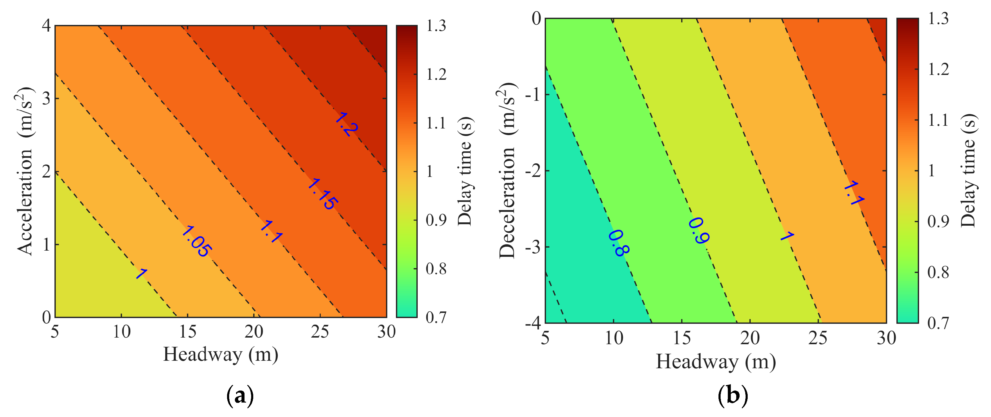
To quantify and visualize this Symmetry Breaking, the theoretical distribution of delay time in the phase plane of spacing headway and acceleration was calculated according to Equation (8), as shown in Figure 4.

Figure 4 clearly reveals the asymmetric characteristics of the delay time distribution, and its physical mechanism can be analyzed from the following two dimensions. First, there is a significant difference in the baseline delay. According to the empirical study by Ozaki [34], the baseline delay coefficient in the acceleration phase (0.886) is significantly higher than that in the deceleration phase (0.743). Reflected in the acceleration phase plane of Figure 4a, the delay time generally maintains a high level (warm color area, approximately 0.9–1.3 s); while in the deceleration phase plane of Figure 4b, the delay time decreases significantly (cool color area, approximately 0.7–1.0 s). This indicates that under the same spacing headway, drivers have a larger inherent lag in executing acceleration commands. Second, the driver’s sensitivity to changes in spacing headway presents asymmetry. In Equation (8), the sensitivity coefficient to spacing headway in the deceleration phase (0.016) is twice that in the acceleration phase (0.008). This means that during deceleration, drivers are more keenly aware of the shrinking gap and can adjust the vehicle speed more quickly through the brake pedal. In contrast, during acceleration, drivers tend to adjust the throttle smoothly to maintain comfort, and their response to the widening gap is relatively sluggish.

This asymmetric mechanism of sluggish acceleration and agile deceleration conforms to realistic driving psychology and vehicle dynamics characteristics. It is this response asymmetry at the microscopic level that acts as a self-adaptive damper in the traffic flow system, effectively inhibiting the propagation and amplification of disturbances.

5.2. Microscopic Asymmetry: Starting and Braking

To verify the specific performance of the aforementioned asymmetric delay mechanism at the level of single-vehicle interaction, this section designs two typical scenarios: vehicle starting (acceleration process) and braking (deceleration process) for numerical simulation. These two scenarios correspond to different regions in the phase plane, effectively testing the dynamic behavior of the model under the asymmetric response field.

5.2.1. Starting Process

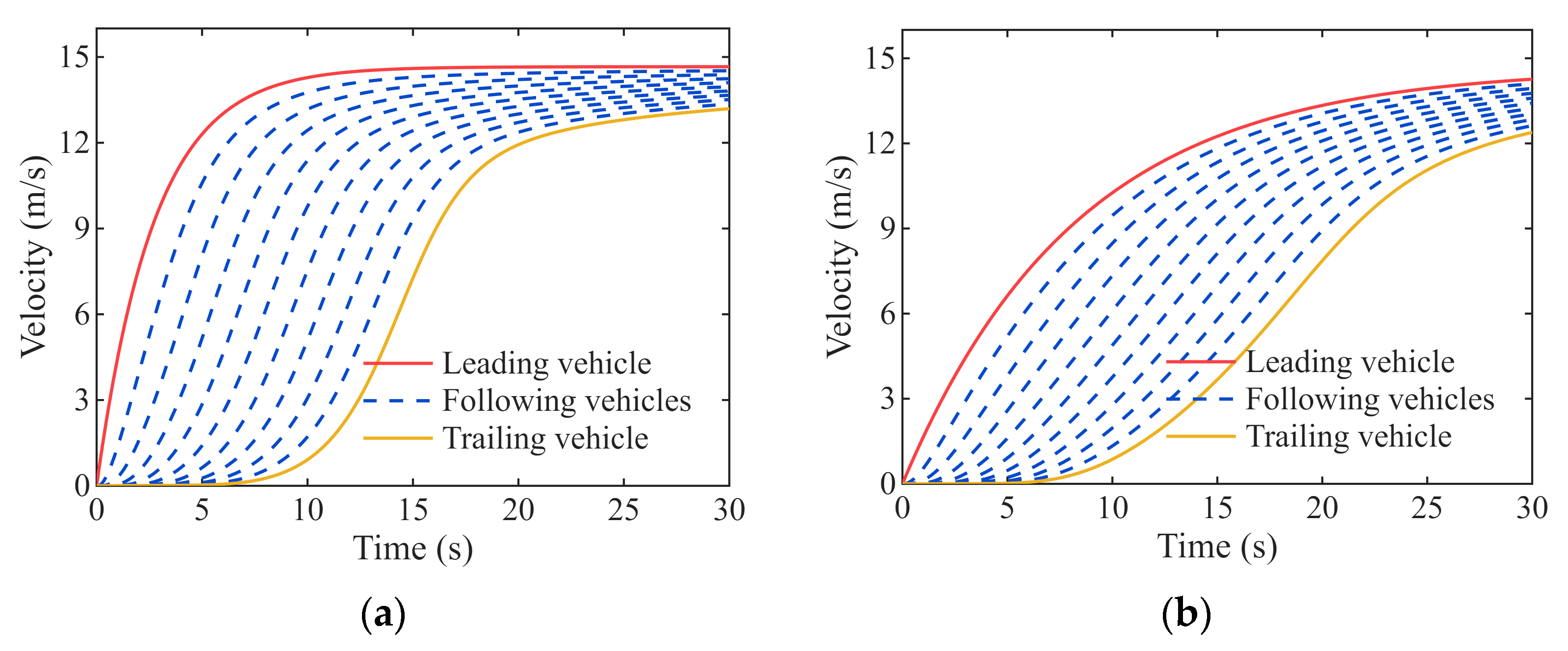
The initial simulation conditions for the starting process are as follows: a car-following platoon of 11 vehicles stops at the rear of the intersection parking line, and the spacing headway between vehicles is 7.4 m. The platoon starts and accelerates to the set maximum velocity when the traffic signal turns green. The instantaneous velocity of the platoon for the first 30 s can then be obtained, as shown in Figure 5.

Significant dynamic differences can be observed from Figure 5. In the FVDM (Figure 5a), the acceleration response of the vehicles is relatively rapid. In contrast, the DACM (Figure 5b) exhibits a distinct hysteresis effect. Combined with the mechanism analysis in Section 5.1, the starting process mainly occurs in the acceleration phase region shown in Figure 4a, where the higher baseline delay and lower spacing sensitivity jointly lead to the sluggish characteristics of the vehicle when starting. This characteristic manifests macroscopically as a reduction in the propagation speed of the starting wave, objectively serving to smooth the traffic flow and avoid sudden acceleration.

5.2.2. Braking Process

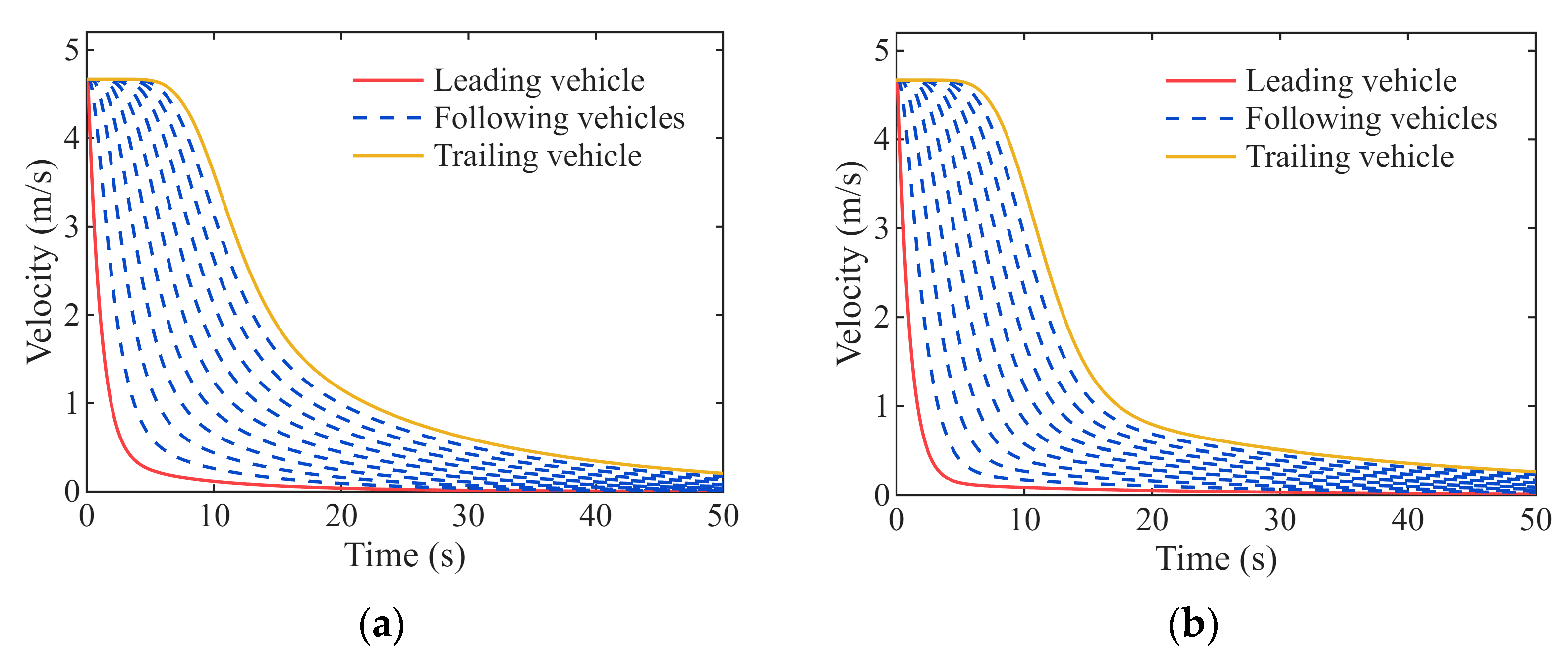
The initial simulation conditions for the braking process are as follows: a car-following platoon of 11 vehicles is uniformly distributed on a single-lane road with a spacing headway of 15 m, and the initial velocity is the optimal velocity at $t=0$. A set of traffic signals is located downstream of the road. The traffic signal turns red, and the platoon starts to decelerate gradually until the leading vehicle stops completely behind the parking line at $t=100$ s. The instantaneous velocity of the platoon for the first 50 s is obtained, as shown in Figure 6.

In sharp contrast to the starting process, the DACM demonstrates high agility in the braking scenario. Observing the velocity curves in Figure 6, the deceleration response of the following vehicles in the DACM is more timely, closely following the changes in the preceding vehicle. The deceleration curves in Figure 7b further confirm that the peak deceleration of the DACM appears significantly earlier than that of the FVDM.

This reversal of dynamic behavior is a direct manifestation of symmetry breaking: when the vehicle enters the deceleration phase, the system automatically switches to a response mode with low delay and high sensitivity. This mechanism ensures that vehicles can make an instant response when facing rear-end collision risks, thereby effectively guaranteeing driving safety.

5.2.3. Quantification of Asymmetry

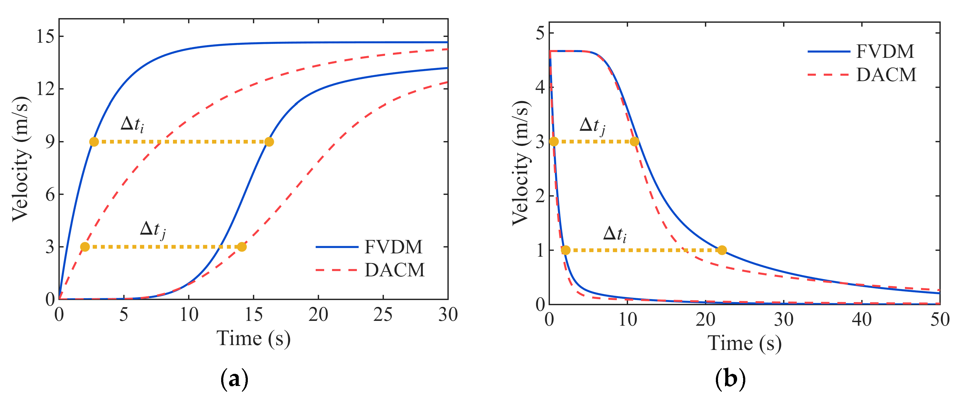
To quantitatively verify the asymmetric mechanism proposed in Section 5.1, this section introduces a dynamic response indicator $∆t$, defined as the time required for the trailing vehicle to reach the same velocity as the leading vehicle (Figure 7). This indicator directly reflects the propagation efficiency of traffic signals within the platoon and the degree of response lag. We selected typical velocity nodes in both the starting and braking processes for statistics, and the results are shown in

Table 3. Time difference between leading and trailing vehicles to reach the same velocity.

Velocity (m/s)	Starting (s)		Velocity (m/s)	Braking (s)
	$∆{\mathit{t}}_{\mathit{i}}$ (FVDM)	$∆{\mathit{t}}_{\mathit{j}}$ (DACM)		$∆{\mathit{t}}_{\mathit{i}}$ (FVDM)	$∆{\mathit{t}}_{\mathit{j}}$ (DACM)
3	11.7	12.1	4	8.7	8.5
6	12.8	13.4	3	10.9	10.3
9	13.5	13.4	2	13.4	12.1
12	15.5	13.7	1	20.0	15.4
Mean	13.4	13.2	Mean	13.3	11.6

.

The data in Table 3 reveal the asymmetric dynamic characteristics of the DACM under different motion states. First, in the early stage of starting, the DACM exhibits obvious hysteresis. Observing the low-speed stage of the starting process (3 m/s and 6 m/s), the time differences in the DACM are all larger than those of the FVDM. This implies that in the initial stage of starting acceleration, the trailing vehicle in the DACM requires a longer time to follow the velocity change in the leading vehicle. This phenomenon coincides with the high-delay mechanism revealed in Figure 4a of Section 5.1, proving that in the acceleration phase, the combined effect of higher baseline delay and lower sensitivity makes the platoon behave more robustly during the starting stage, effectively smoothing violent velocity fluctuations.

Secondly, in the braking process, the DACM exhibits significant agility. At all velocity nodes in the braking process, the time differences in the DACM are significantly smaller than those of the FVDM. Especially when the velocity drops to 1 m/s, the moment just before stopping, the response time of the DACM is shortened by 23% compared to the FVDM. In terms of the average value, the braking response time difference in the DACM is significantly superior to that of the FVDM. These data powerfully prove that in the deceleration phase, the low-delay mechanism (see Figure 4b) is effectively activated, enabling vehicles to transmit braking signals with extremely high efficiency, thus macroscopically manifesting as safer car-following spacing control.

In summary, the quantitative results in Table 3 confirm that the DACM successfully reproduces the temporal asymmetry in real driving behaviors: providing lag damping during the acceleration stage where smoothness is needed, and providing instant response during the braking stage where safety is needed. This state-dependent dynamic switching is the physical essence of why the proposed model is superior to traditional fixed-parameter models.

5.3. Macroscopic Symmetry Breaking: Oscillation Suppression

Numerical simulations are performed under periodic boundary conditions in this section to analyze the impact of the dynamic delay on the car-following behavior. The simulation scenario and initial small perturbation settings are the same as those in the literature [44]. Specifically, the simulation is conducted on a circular road with a total length of $L=1500$ m. The total number of vehicles is set to $N=100$, resulting in an initial uniform spacing headway of $b=L/N=15$ m. Initially, all vehicles move at the steady-state velocity $V\left(b\right)$. At $t=0$, a perturbation of magnitude 1 m is applied to the positions of the 50th and 51st vehicles to disrupt the equilibrium, while the remaining vehicles maintain their steady-state conditions.

5.3.1. Instability Induced by Fixed Symmetric Delay

It is essential to analyze the effect of delay on FVDM performance and verify its consistency with actual situations, since delays are unavoidable in realistic car-following processes. In addition to analyzing the dynamic performance of the FVDM at $T=0$ s, we also investigate the effect of different fixed delay times. The fixed delay time ($T$) is added to the spacing headway term in the FVDM to be consistent with the DACM. Note that Equation (10) shows that the DACM degenerates to the FVDM when $T\left(∆x,a_n\right)=0$ s but with different parameter values. Thus, we select the parameter combination of $k=0.36$ and $\lambda =0.84$ for the FVDM, and $k=0.12$ and $\lambda =0.97$ for the DACM to explore the impact of different delay times on their dynamic performance under the small perturbation. 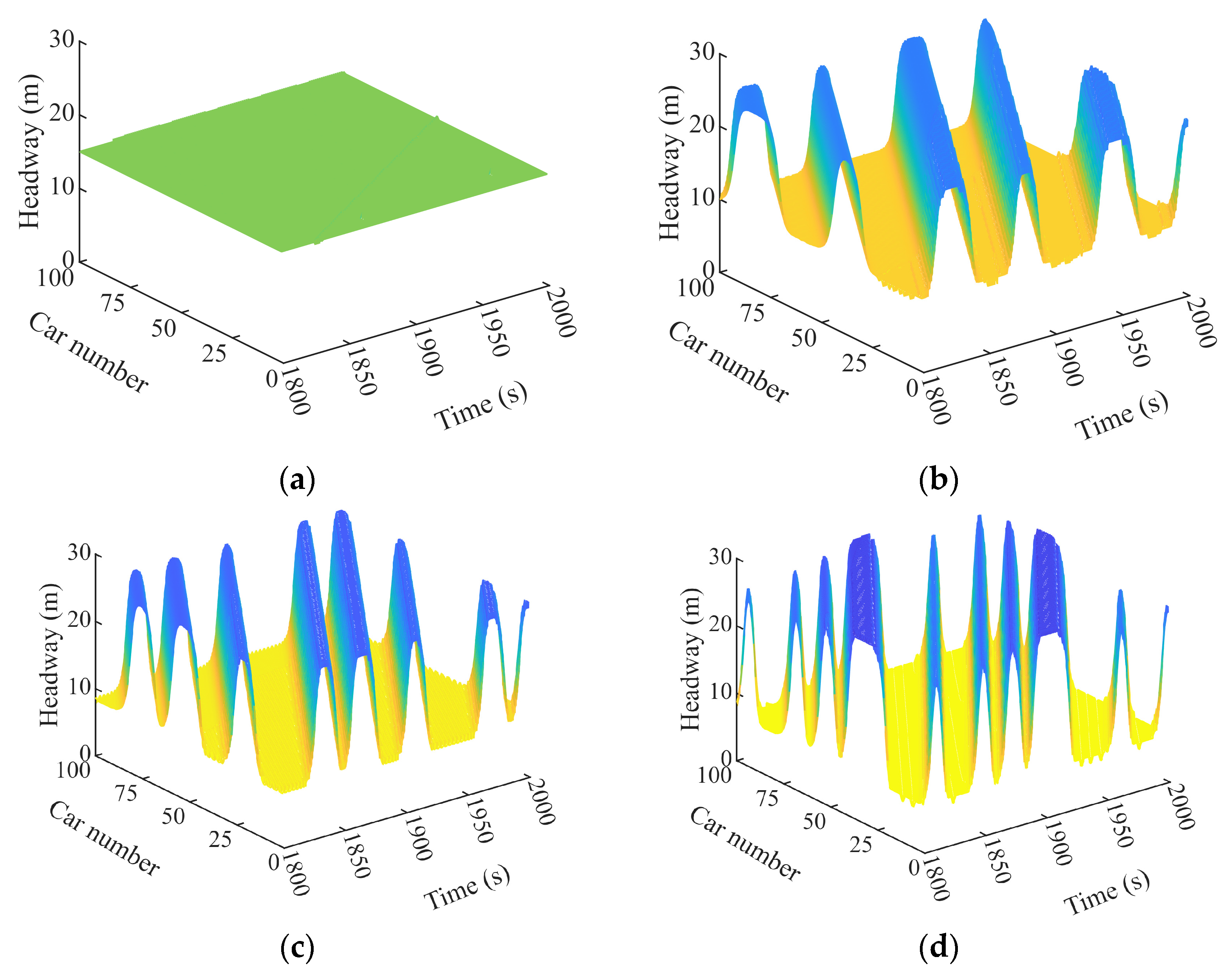Figure 8 shows the spatiotemporal evolution of the spacing headway of the FVDM under different fixed delay times.

From Figure 8a, it can be seen that when the delay effect is ignored ($T=0$), the FVDM is capable of absorbing the initial perturbation, and the traffic flow rapidly recovers to a uniform steady state. However, with the introduction and increasing value of the fixed delay time (Figure 8b–d), the system gradually loses stability. Particularly when $T \ge 1.0$ s, the spacing headway exhibits violent periodic oscillations, and the amplitude of these oscillations amplifies over time, eventually forming stop-and-go waves. This instability phenomenon reveals the drawback of temporally symmetric delays. Since the model adopts identical delay parameters during both acceleration and deceleration phases, the system fails to break the closed loop of energy accumulation. When the driver attempts to adjust the spacing headway through acceleration or deceleration, the fixed delay leads to continuous overshoot, thereby macroscopically inducing symmetric traffic oscillations.

5.3.2. Suppression Mechanism via Asymmetric Delay

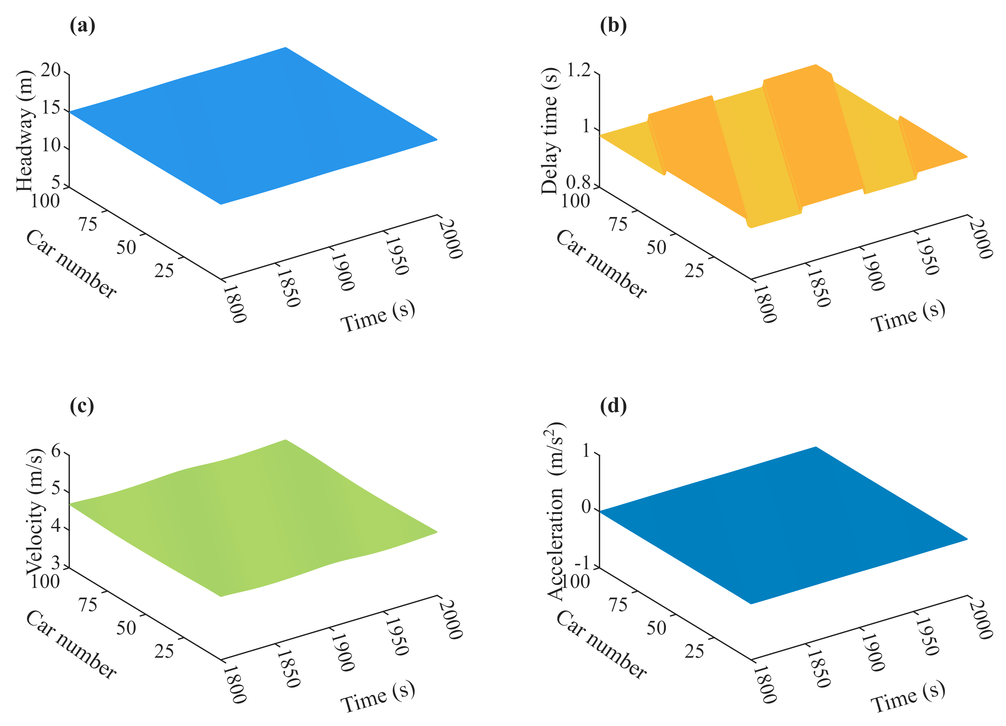
To validate the performance of the calibrated model, we conducted numerical simulations identical to those of the FVDM to investigate the stabilizing effect of the asymmetric delay mechanism on traffic flow. Figure 9 illustrates the temporal evolution trends of headway, dynamic delay, velocity, and acceleration under the asymmetric delay mechanism.

Figure 9a,c,d show that the initial disturbance was completely absorbed by the system after considering the asymmetric delay mechanism, and no traffic congestion occurred, fully demonstrating the strong anti-interference capability of the proposed model. Figure 9b directly shows the core contribution of the proposed model, namely, the delay time in the DACM is dynamically changing and actively adjusts the delay according to traffic conditions. Furthermore, it can be seen that the dynamic delay time fluctuates between 0.8 s and 1.2 s, with an average of approximately 1.0 s. Based on this, we compared the performance difference with that of the FVDM with a fixed delay of 1.0 s. The headway fluctuation amplitude can fully characterize the severity of traffic flow oscillations. We calculated the maximum amplitude and standard deviation of the headway fluctuation during the oscillation development stage (t > 1500 s). The calculation results show that the amplitude of the fixed-delay FVDM is 18.4 m, and the standard deviation of the velocity is 5.12 m/s, exhibiting severe oscillations. In contrast, the DACM effectively suppressed these disturbances, causing the oscillation amplitude and velocity fluctuations to decay rapidly to negligible levels, thereby maintaining a stable traffic flow. This result strongly confirms the superior ability of the calibrated DACM in stabilizing traffic flow.

We must acknowledge that the above results were obtained under a specific combination of calibrated parameters. To investigate whether the optimal parameter combination or the asymmetric mechanism was the cause, we designed an ablation experiment to compare the ability of symmetric and asymmetric mechanisms to suppress traffic congestion and resist interference under the same parameter settings. For the asymmetric mechanism, the dynamic asymmetric delay function in Equation (8) was retained. For the symmetric delay mechanism, we unified the dynamic delay using the calculation logic from the acceleration mode, with the constant term set to the average of the acceleration and deceleration modes. This setup is discussed in Section 3.3. 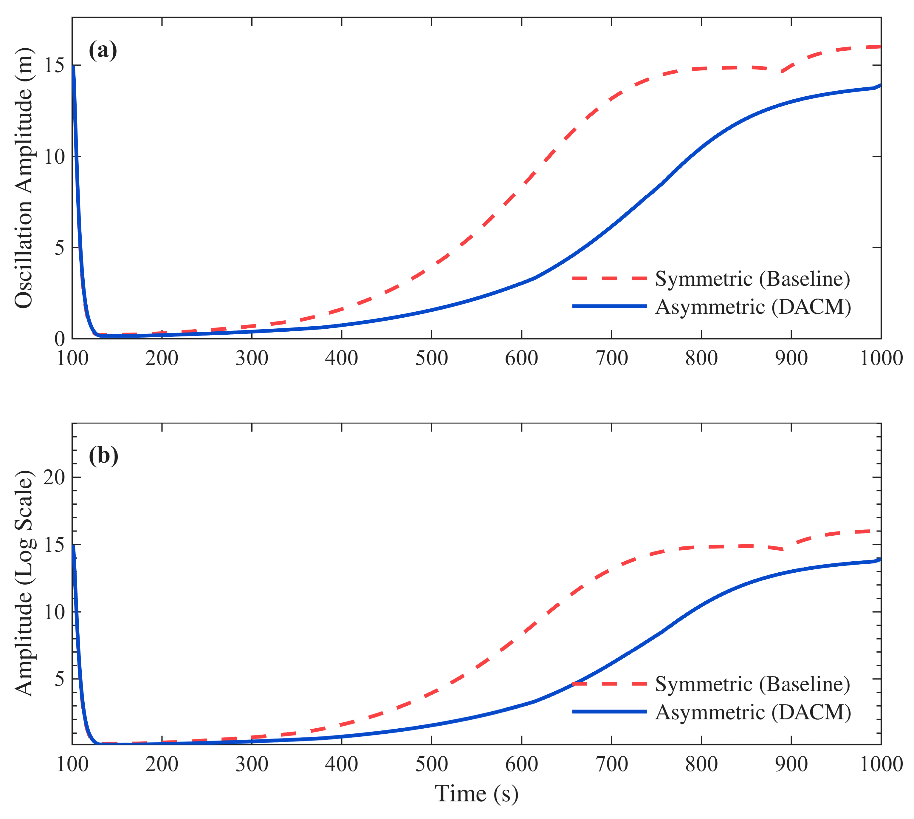Since the calibrated parameters were overly robust in suppressing congestion, and to clearly observe the differences between the two mechanisms, we adjusted $\lambda$ to 0.8 while keeping other parameters unchanged. This enables us to observe the performance difference between asymmetric and symmetric mechanisms under more adverse traffic conditions. We repeated the numerical simulation and obtained the results shown in Figure 10.

As clearly observed in Figure 10a, under adverse traffic conditions, the simulated traffic flows under both mechanisms exhibited oscillations and rebounds after 300 s. However, the oscillation amplitude of the symmetric delay mechanism was significantly greater than that of the asymmetric mechanism. At t = 600 s, the oscillation amplitude of the traffic flow under the symmetric delay mechanism reached approximately 8.0 m, while that under the asymmetric delay mechanism was only about 2.5 m. In comparison, the asymmetric delay mechanism effectively suppressed traffic oscillations. Furthermore, on a logarithmic scale, the slope of the curve reflects the exponential growth rate of the disturbance. Observing Figure 10b, it can be seen that the exponential growth rate under the asymmetric delay mechanism is much smaller than that under the symmetric delay mechanism, which further demonstrates that the asymmetric delay mechanism can effectively suppress traffic congestion. That is, the asymmetric delay mechanism plays a core role in suppressing traffic oscillations within the model architecture.

It is worth noting that in Section 2.2, we specified that the threshold $ϵ$ for the hysteresis switching mechanism was set to $0.1\times {10}^{-3}$ m/s². This setting aims to avoid frequent switching between acceleration and deceleration modes near the zero point of acceleration during numerical calculations or when substituting real data. Based on the ablation experiments described above, we further conducted robustness tests on $ϵ$. Specifically, under the asymmetric delay mechanism, we performed numerical simulations with $ϵ$ at different orders of magnitude, and the results are shown in

Table 4. Robustness of simulation results under different hysteresis switching thresholds.

	$\mathit{ϵ}$ (m/s2)	Oscillation Amplitude (m)	Deviation
Baseline	$0.1\times {10}^{-3}$	3.0359
Case A	$0.1\times {10}^{-2}$	3.0185	0.57%
Case B	$0.1\times {10}^{-4}$	3.0370	0.04%

.

Experimental results show that the amplitude of traffic oscillations did not change significantly under different thresholds. This indicates that the choice of threshold does not affect the severity of traffic congestion; rather, the asymmetric delay mechanism plays a suppressive role. In conclusion, the introduction of the asymmetric delay mechanism into car-following control is essential and has a positive effect on traffic flow stability.

6. Conclusions and Discussion

This paper addresses the limitations of the temporal symmetry assumption implied in traditional car-following models by constructing an improved delay adaptive car-following model that considers the asymmetric dynamic delay characteristics of drivers and vehicles. By introducing a state-dependent dynamic delay function, the proposed model mathematically breaks the response congruence between acceleration and deceleration processes. It not only successfully decouples the mixed effects of sensitivity parameters and delay effects found in traditional models but also endows the model with the capability to describe complex hysteresis phenomena in realistic driving behaviors.

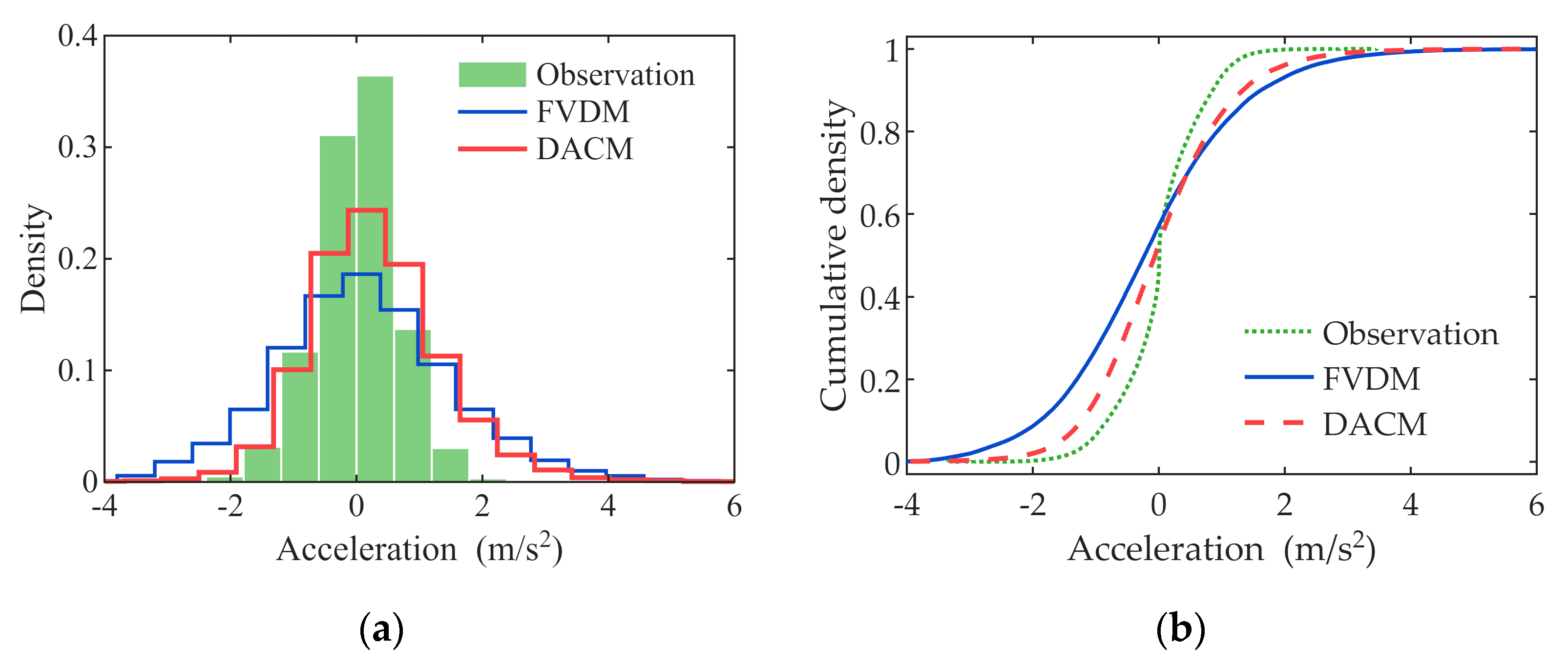
Calibration and validation results based on empirical trajectory data from the Next Generation Simulation program indicate that the delay adaptive car-following model is significantly superior to the classic full velocity difference model in reproducing microscopic vehicle motion characteristics. The study confirms that real driving behaviors exhibit significant characteristics of sluggish acceleration and agile deceleration, and this microscopic symmetry breaking mechanism is accurately quantified in the delay adaptive car-following model. Specifically, during vehicle starting and acceleration phases, the model exhibits larger delays and lower sensitivity, serving as a damper to smooth velocity fluctuations. Conversely, during braking and deceleration phases, the model automatically switches to a low-delay and high-sensitivity mode, ensuring instant response to the deceleration signals of the preceding vehicle and guaranteeing driving safety. Linear stability analysis and numerical simulations of macroscopic traffic flow evolution further reveal the profound physical mechanism of the asymmetric delay. Comparative analysis shows that the fixed symmetric delay in traditional models is often a key factor that destroys system stability and induces the evolution of small perturbations into severe stop-and-go waves. In contrast, the delay adaptive car-following model dynamically adjusts the response lag under different motion phases and effectively dissipates disturbance energy by utilizing the high-delay characteristics during the acceleration process, thereby significantly suppressing the generation of traffic oscillations at the macroscopic level. This finding powerfully demonstrates that incorporating the temporal symmetry breaking mechanism into car-following dynamic equations plays a crucial role in enhancing the robustness of the traffic flow system against delays.

We must acknowledge the limitations of this study. The current numerical simulation is based on an idealized single-lane homogeneous traffic environment. In reality, traffic heterogeneity (such as mixed vehicle types with different delay characteristics), lane-changing behavior, and signal control at intersections introduce additional complexity that may affect the stability boundary. Future research will extend the proposed model to these complex scenarios to further validate the robustness of the asymmetric delay mechanism. Additionally, the proposed mechanism has significant practical application potential in connected and autonomous vehicle systems. Specifically, the asymmetric acceleration delay logic can be integrated into the algorithm design of adaptive cruise control (ACC) and cooperative adaptive cruise control (CACC). By mimicking this human-like asymmetry, the automatic controller can effectively act as an oscillation damper, thereby enhancing queue stability and passenger comfort in mixed traffic flows.