Abstract
The population activity of grid cells from a single module is topologically constrained to a toroidal manifold. Our work proposes an improved version of Gardner’s earlier model, which can account for both geometric properties and force field dynamics. Employing methods from Differential Geometry, we have derived Lagrangian densities that—under very general assumptions and avoiding dimensionful constants—provide a rationale for the trajectories associated with the synaptic spacetime as a global solution to the Einstein–Maxwell field equations. Then, we investigate the helical solutions to show that the synaptic toroidal topological space, as a locally flat Minkowski spacetime, with a Lorentzian metric is geodesically complete and, therefore, exhibits maximal stability. Finally, we consider a Lorentzian metric with curved spacetimes that give rise to Lorentzian tori admitting curvature spacetime singularities.
1. Introduction
Gardner et al. [1] demonstrated that the population activity of grid cells—an essential component of the visual nervous system (VNS)—is reliably confined to a low-dimensional manifold with toroidal topology, wherein the dynamics of neural activity closely track an animal’s movement through physical space. More specifically, they showed that the attractor of the dynamical system formed by the population activity of a grid cell module is topologically equivalent to a torus. This toroidal representation was shown to be invariant across different environments and brain states, offering important insights into the underlying mechanisms governing visual cortex neuron dynamics. Notably, this finding is independent of the specific grid cell sample chosen, its size, or the experimental conditions under which the experiment is conducted, thus establishing it as an invariant feature of the grid cell system [2]. However, the nature of the network architecture that sustains this topology remains unresolved [3]. Specifically, it is still unclear whether the toroidal manifold reflects a preconfigured geometric organization or emerges from initially random connectivity that is shaped through experience-dependent synaptic plasticity.
In previous work [4], we proposed a geometric framework for modelling synaptic brain dynamics based on Lorentzian manifolds. This approach deliberately omits several details related to spatial irregularities and the microscopic temporal evolution of fields, which remain beyond the reach of current experimental measurement. Within this framework, we developed a covariant formulation of Maxwell’s equations, including a generalized Ohm’s law suitable for media with non-uniform and highly anisotropic properties, characterized by conductivity tensors with non-zero off-diagonal components.
Then, we study two previously unrelated findings: (i) the torus as the topological space associated with the VNS, and (ii) the observation that spiral waves are a ubiquitous and natural mode of communication among neurons [5]. We demonstrated that these two aspects are intrinsically linked through specific topological and geometric constraints imposed on the corresponding Lorentzian manifold. In particular, we showed that stable circular helices arise as geodesics—solutions to the path-minimization problem—within the toroidal manifold [6].
Within the work provided by Gardner et al., the validity of the toroidal description was assessed by comparing statistical measures of how well toroidal coordinates accounted for neural activity both on the torus and in physical space in the context of continuous attractor networks (CANs). To examine the structure of the grid cell population activity for signs of toroidal topology, they constructed a three-dimensional embedding of the n-dimensional activity of a module of = 149 pure grid cells. This was achieved by applying a two-stage dimensionality reduction procedure to the firing-rate matrix. The spatial offsets of individual cells in the arena matched the relative firing locations of the cells in the toroidal state space.
The concept of a continuous attractor network (CAN) has emerged as one of the most influential frameworks in theoretical systems neuroscience. However, in the case of grid cells, the sheer number of possible locations in the two-dimensional state space has thus far prevented a clear identification of the underlying manifold topology. To address this limitation, we propose employing geometric and topological methods from Einstein–Maxwell theory in curved spacetime. On the inferred torus, individual grid cells display distinct firing fields. Toroidal coordinates for the population activity vector are then incorporated into a Lagrangian, with parameters linked to the mean firing rate of a grid cell as a function of its toroidal position.
In this paper, we propose a Lagrangian approach to deriving energy-preserving finite difference schemes for Euler–Lagrange partial differential equations. The Lagrangian formulation provides general and elegant frameworks for mechanics, unifying the treatment of diverse mechanical systems. Symmetries and conserved quantities are central in the analysis of particle and rigid-body dynamics [7,8]. Within our approach, we explore the geometric structure of differential equations, including the inverse problem of the calculus of variations.
Mathematical models aimed at describing the dynamics of electromagnetic fields in the brain should take into account the inherently irregular and non-uniform anisotropy. Yet, no mathematical framework has been formulated that adequately reflects the influence of the brain’s multiscale structural discontinuities—identified through histological analysis—on electrophysiological behaviour. Here, we propose a solution derived from the coupled Einstein–Maxwell field equations (with source charges and currents) in four spacetime dimensions. Then, we derive all the metric and Maxwell field components, together with explicit constraints imposed by the field equations [9].
In spacetime , with , a connected 4D manifold and , a Lorentzian metric, physical fields represent matter content. These fields follow equations involving tensors on , where differentiation is defined via the covariant derivative compatible with . The dynamics of matter imply the existence of a symmetric energy–momentum tensor , relating geometry and matter through Einstein’s field equation [10],
is the cosmological constant, is the Ricci tensor, is its trace, and . The tensor incorporates contributions from the fields and their covariant derivatives. The Einstein–Maxwell equations constitute a regularized form of Maxwell’s theory within nonlinear electrodynamics, admitting numerous significant geometric solutions in the framework of General Relativity. In the Einstein–Maxwell system, the field equations (without ) are paired with , where includes the Maxwell stress–energy tensor, alongside the generally covariant Maxwell equations [11,12].
A major obstacle in efforts to incorporate this geometric framework with Maxwell’s equations stems from the fundamental differences in their formulation. Maxwell’s equations, developed within the context of Special Relativity, describe fields propagating on a fixed Minkowski spacetime background. General Relativity, by contrast, treats the force field not only as the mediator of a fundamental interaction but also as the entity that fundamentally determines the geometry of spacetime. Thus, unlike electromagnetism, where the background is fixed and independent of the field, in General Relativity, the field and the background are the same: the spacetime metric [13].
An additional conceptual challenge arises from the fact that the treatment of matter in General Relativity is fundamentally different from that in Maxwell field theory on a fixed, flat (Minkowski) background. In the absence of a unique global time parameter, it is not evident how to define an inner product that remains invariant under time evolution. The lack of a preferred foliation leads to an intertwining of kinematical and dynamical structures when the background geometry is curved [14]. At the foundational level, one starts with a set of abstract points that must be related to physical spacetime events. This set must be endowed with a topology—toroidal in the case under consideration—and a differentiable structure that equips it with the properties of a smooth manifold. Furthermore, even in semiclassical approximations where the background geometry is fixed and one studies only the influence of matter on it, a dimensional coupling constant appears in the action, introducing additional difficulties in the formulation and interpretation of the theory [15].
The Einstein field equations, which govern the evolution of the force field, are purely differential in nature. Their solutions determine the local geometry of spacetime but do not constrain its global topology. A manifold endowed with the metric that satisfies Einstein’s equations may, in principle, support multiple distinct topologies. Nevertheless, unless stated otherwise, the literature generally assumes manifolds that are connected, Hausdorff, compact, and smooth (), with no boundary [16]. Even in the simplest case—where the field equations yield a completely flat manifold (i.e., with a vanishing Riemann tensor everywhere)—the global topology need not be Euclidean.
This work seeks to address several outstanding questions by determining the appropriate form of the Lagrangian, at least within a semiclassical framework; examining the impact of observer-related modifications on the formulation; and identifying a suitable potential function in the context of the Einstein–Maxwell equations, particularly in relation to how the electromagnetic tensor affects the underlying toroidal manifold.
So, we constructed a topological relativistic field theory within the Einstein–Maxwell equations, which was formulated to address the Lagrangian dynamics of VNS-inspired toroidal manifolds. The development relies entirely on differential geometric methods, employing the Weyl formalism to encode both the metric and gauge structures [17]. The associated observables were derived, revealing a nontrivial set of topological invariants that characterize the underlying geometry. This formulation offers a novel perspective on the interaction between curvature, topology, and field dynamics in complex manifolds relevant to geometric modelling in neuroscience.
The paper is organized as follows: In the Preliminary Section, the family of cylindrical and toroidal differentiable manifolds is presented. Initially, in the Results and Discussion Section, we discuss the geometric and topological aspects of the Einstein–Maxwell fields in flat spacetimes. We constructed a Lagrangian to analyse the synaptic stability of helical geodesics in Einstein–Maxwell toroidal field equations. Subsequently, we also consider the geodesic completeness and curvature of spacetime singularities on the Lorentzian torus in curved spacetimes. Finally, the conclusions are presented.
2. Preliminary
2.1. Toroidal and Cylindrical Differentiable Manifolds
Differential geometry investigates geometric objects (manifolds) through the methods of analysis and algebra. Manifolds constitute the fundamental objects of study, as they generalize notions such as curves and surfaces while locally exhibiting the structure of Euclidean space. Einstein’s general theory of relativity characterizes gravitation not as a force but rather as the curvature of spacetime induced by matter and energy, with manifolds serving as the mathematical framework—specifically, four-dimensional pseudo-Riemannian or Lorentzian manifolds—that enable the modelling of this curved spacetime.
It can be shown that every finite-dimensional manifold over can be embedded into [18] for sufficiently large . One of the main problems in differential topology is determining the minimal , for which such an embedding exists for a given manifold . In the case of the torus, a two-dimensional manifold, it can be embedded directly into . In the following, we define a differentiable manifold structure on the cylinder (finite or infinite) and on the torus.
2.1.1. Finite Cylinder
The finite cylinder of radius and height is projected onto an annular region in the plane,
Then,
It is a differentiable manifold with a single chart.
2.1.2. Infinite Cylinder
It becomes a finite cylinder of height simply by previously defining the homeomorphism,
Ultimately, the projection is now
Once again, it constitutes a differentiable manifold characterizable by a single chart.
2.1.3. Torus (
The toroidal coordinates are defined by
By making two local cuts (Figure 1), it is transformed into two cylinders, each of which is a one-chart manifold. Consequently, the torus can be described using two local charts.

Figure 1.
A torus with two cuts representing the compactification of the cylinder.
Another representation: the torus is obtained from a square by identifying each side with its opposite (Figure 2).
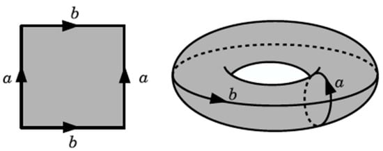
Figure 2.
The torus can be constructed by identifying the sides of the square and continuously deforming it; every open set on leads to an open set on . A torus is defined by two key parameters: the major radius () and the minor radius ().
The standard parametric equations of the circular helix with radius and pitch are as follows:
This describes a curve that spirals around the -axis, with the and components forming a circle of radius , while the component increases linearly with , representing the helix’s vertical rise.
With the following explicit Lorentzian metric for the toroidal manifold,
Geodesics on a cylinder are helical curves (helices). On the circular cylinder defined by , the geodesics include cross-sectional circles formed by the intersection of planes parallel to the xy-plane with the cylinder, as well as straight lines parallel to the -axis (helices) (see Figure 3). To determine the geodesics, we utilized the isometry that maps to .

Figure 3.
The right circular cylinder of radius and height . The point M on the helix is defined by helical coordinates .
3. Results and Discussion
3.1. Geometric and Topological Aspects of the Einstein–Maxwell Equations in Flat Spacetime
The initial formulation of the Einstein–Maxwell equations involves considering a flat metric that decomposes into a Minkowski background metric , plus a perturbation tensor , which represents deviations from this flat geometry. Thus,
This decomposition allows for the recovery of a flat background possessing all the symmetries of the Poincaré group, which are essential for a relativistic field theory within Special Relativity, along with the existence of privileged reference frames. However, the question arises as to what ensures that the manifold possesses metric properties sufficiently close to those of Minkowski spacetime to allow such a decomposition, given that the proposed metric assumes to be a perturbation of a flat background. In practice, performing this decomposition requires the manifold to have topological properties similar to those of flat spacetime. Yet, topology remains entirely undetermined within the framework of General Relativity [19,20].
Nevertheless, this generalization entails several difficulties. In particular, a complication arises when attempting to express the Einstein–Maxwell Lagrangian explicitly: one finds that the theory involves not a single tensor, but two: the metric and its inverse . This dual structure renders the theory intrinsically non-polynomial, unless one introduces a background-perturbation decomposition or adopts a suitable parametrization scheme [21,22]. The proposed changes to the Einstein–Maxwell equations consist of (1) replacing the gravitational side with a scalar term added to the electromagnetic sector and (2) introducing a nonlinear, four-dimensional electromagnetic constitutive tensor.
3.2. Dimensional Analysis
To satisfy the requirements of dimensional analysis, only those functions of physical quantities will be admissible that transform under a scale transformation of ratio according to the following rule: if , ,…, have dimensions , ,…, , then any function , ,…, with dimensions that can be formed from them must satisfy
This is the only imposed restriction. It prohibits the presence of dimensionful constants in the theory.
Aldersley demonstrates the following two theorems in his work [23]:
- Let be a class tensor concomitant of the metric and its derivatives up to any order,such that its dimensions are , and assuming that condition (2) is satisfied—which is, in fact, an axiom of the theory—then, for a four-dimensional manifold, it holds thatis the curvature scalar and is the electromagnetic field tensor, such thatwhere is the Lagrangian.
- Let be a scalar density of class , concomitant of the metric and its derivatives up to the arbitrary ordersuch that its dimensions are , and assuming that axiom (2) is satisfied. Then, it follows that the manifold is four-dimensional, since
For both proofs, Aldersley employs arguments similar to those described so far, together with Lovelock’s theorem [24]: If is a tensorial concomitant satisfying , then, in a four-dimensional manifold,
If dimensional constants had been permitted in —for example, with —the absence of the differentiability properties of with respect to (and the same holds for any tensor, not just density ) would have rendered the entire analysis presented above impossible.
If, instead of choosing two universal constants with dimensions that relate lengths, times, and charges as per Aldersley ( and ), it is considered that three universal constants exist, for example , , and with , , this would lead to the time scale being proportional to itself, satisfying the relation,
where is a dimensionless constant.
The restriction of excluding dimensionful constants from the theory—aside from the aforementioned two universal constants relating length, time, and mass—does not affect the derivation of the Lagrangian densities for the Einstein–Maxwell fields. In particular, no dimensionful constants are introduced in the Lagrangian, and the cosmological constant Λ is treated as a variable, which may become constant only in specific cases. The remaining parameters appearing in the Lagrangian (, ,…, ) are regarded as dimensionless constants.
3.3. Einstein–Maxwell Lagrangian Formulation
In the formulation of Lagrangian densities, it is natural to employ the classical theory of concomitants, which studies the general form of mathematical entities depending on the field variables and their derivatives, combined with dimensional analysis. This approach is justified because the equations of motion for the various fields involved in the Lagrangian formulation of a theory can be derived by applying a variational principle to the action constructed from the corresponding Lagrangian density, which is a function of the fields and their derivatives. The outcome of applying the variational principle is the Euler–Lagrange equations, and it has been demonstrated that these expressions are concomitant operators [25].
Weyl’s theorem states that the most general Lagrangian density that can be constructed from the metric and its derivatives up to the second order and that is linear in the second derivatives is the Einstein Lagrangian. Rigorous studies have been conducted on the Lagrangians commonly employed in semiclassical theories [26], as well as on more general possible Lagrangians [27]. The resulting field equations derived from the variation of the Lagrangian density must be gauge-invariant under the appropriate symmetry group.
Hypothesis:
The precise formulation of this hypothesis is summarized as follows:
- (i)
- The Lagrangian density to be constructed must be a function of the metric , the electromagnetic vector potential , and a scalar field . The latter may be either a conventional field or a constant.
- (ii)
- No dimensional constants are allowed in the Lagrangian, as their presence generally leads to non-renormalizable theories.
- (iii)
- We permit first derivatives of the fields and because we require their field equations to be of the second order. For the metric, both first and second derivatives are allowed. No upper bound is imposed on the order of derivatives in the Lagrangian to keep the theory as general as possible.
- (iv)
- Units are chosen such that and denotes the action. Hence,
- (v)
- Finally, we require gauge invariance for the field equations.
In the subsequent development, the powers of the arbitrary degree of the fields and their derivatives will be admitted. We shall allow only derivatives of and so that the resulting field equations for them are of the second order and the second derivatives of , since it is not possible to construct a concomitant other than a constant using only the metric and its first partial derivatives. In any case, the Hilbert action is degenerate, and consequently, the field equations for the Einstein–Maxwell system derived from it are of the second order, even though the Lagrangian density itself is of the same order.
The correct units of and are obtained by inspecting the units of their kinetic terms in the Lagrangian,
with y
so,
The issue of the dimensionful constant is related to the fact that two tensors, rather than one, are involved in the field action. The perturbative treatment of the field requires its decomposition into a flat background metric plus a perturbation , which must be multiplied by the constant so that the sum carries the correct units. Thus, the decomposition is
The inverse and the determinant expand into an infinite power series in ,
where the position of the indices is irrelevant, since raising and lowering is performed with . In the coordinate gauge for , one has with . Thus, gauge invariance reduces the degree of divergence in the Einstein–Maxwell case, making it sufficient to set several coefficients in the Lagrangian expression to zero.
Lemma 1.
Let
denote the concomitant Lagrangian of the metric tensor, the electromagnetic potential (a covector), a scalar field, and their derivatives up to the order specified in the following equation:
Based on condition (iii) and using the field dimensions expressed in (iv), under a scaling transformation applied to , we obtain
Replacement Theorem.
If satisfies Equation (3), as well as assumptions (i)–(iv), then for real manifold dimension
, the general Lagrangian density is [28]
where
denote numerical constants.
Lemma 2.
By differentiating four times with respect to
, taking the limit
, and applying the replacement theorem, we obtain
where are tensor densities, and the semicolon denotes covariant differentiation with respect to the Christoffel symbols . In a physical problem formulated within the framework of Differential Geometry, the Christoffel symbols correspond directly to the force field governing the physical system under consideration. The underlying differentiable manifold is typically Lorentzian, and particles are assumed to follow geodesic paths, that is, trajectories of stationary action.
Lemma 3.
The tensor densities
have been determined for the arbitrary order [29]. Based on these results, and assuming the spacetime dimension , it is shown that
- (i)
- (ii)
- (iii)
- (iv)
- is a linear combination of and , where the brackets [ ] denote antisymmetrization over the indices enclosed, and denote the concomitants of the metric tensor, which are known in the generic case. For example,
- (v)
- (vi)
- (vii)
- is a linear combination of y
- (viii)
- is a linear combination of y
Observation 1.
In this way, we obtain the following expression for the action:
We now return to the issue of gauge invariance. We require that all field equations, which must have physical significance, remain invariant under local transformations of the group. Thus, suppose that is gauge invariant. Then,
and consequently,
By differentiating Equation (4) with respect to , it immediately follows that . Then, by contracting Equation (4) with and differentiating with respect to , one finds that:
Multiplying by and contracting with , we obtain .
Let us now suppose that is gauge invariant. Then,
which implies that
By differentiating Equation (5) with respect to , and evaluating at a point where the metric takes the form , setting and , and we obtain . Next, taking , , and , it follows that . Finally, with and , we find .
Differentiating Equation (5) with respect to , and taking into account that , we obtain
Now, by setting and, , we find that .
Finally, let us assume that is gauge invariant. Then,
The same applies to
Since is linear in , fourth-order derivatives do not appear in . Finally, by differentiating with respect to and subsequently contracting with , it follows that . In this way, we have established the following,
Theorem 1.
If is a Lagrangian density of the form,
which satisfies hypotheses (i) through (v), then the gauge invariance of the Euler–Lagrange equations imply the gauge invariance of the Lagrangian, which takes the form
The terms , , and can be related in four dimensions () through the Gauss–Bonnet theorem.
Observation 2.
The brain’s spacetime, considered a manifold, constitutes a central theme of the present work. Building on Weyl’s program for the unification of long-range interactions (gravity and electromagnetism), we associate the purely geometric concept of curvature of a Weyl spacetime with the presence of the local cerebral electromagnetic field. General Relativity arises as a particular case of Equation (6) if we allow it to be expressed without dimensional constants in the Brans–Dicke fashion. The Lagrangian of the latter theory can be derived from Equation (6) by choosing , , and setting all other coefficients to zero. General Relativity is then recovered by identifying .
Corollary 1.
Equation (6) enables us to derive the Lagrangian for the Einstein–Maxwell field equations, which we adapt to the Minkowskiian spacetime of the grid cells toroidal manifold by an appropriate choice of constants. The Einstein–Maxwell equations are obtained by replacing the partial derivatives in the Minkowski space formulation with covariant derivatives from Equation (6) by setting , , all other , and identifying .
Observation 3.
However, the application of this Lagrangian entails several difficulties. Among them is the question of what guarantees that the manifold possesses metric properties sufficiently similar to those of Minkowski spacetime to allow for a decomposition such as (1). Furthermore, when treated perturbatively, the powers of the cosmological constant Λ that appear in the expansion lead to a loss of predictability in the theory. In addition, for such a decomposition to be carried out in practice, the manifold must exhibit topological properties akin to those of flat spacetime. Yet, topology remains completely undetermined in General Relativity and in the Einstein–Maxwell equations. In what follows, we shall develop this Lagrangian for a toroidal manifold associated with cerebral synaptic activity and examine its properties.
3.4. Synaptic Stability of Helical Geodesics in Einstein–Maxwell Brain Field Equations
Our previous work [5] aimed to better understand how brain spiral waves arise by studying the geometric properties on regular surfaces of a given topological space where a metric has been incorporated, and specifically, we demonstrated that helices are the only non-trivial geodesics on Minkowskiian tori (Figure 4).
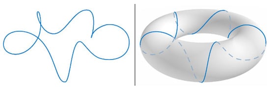
Figure 4.
The circular helix: a helical line (of radius a) coiling around a torus (of radius R) in the x–z plane.
The problem of particle motion can be simplified by considering a central potential and, specifically, by analysing the Lagrangian corresponding to the Lorentz force experienced by a particle in electromagnetic fields. A persistent difficulty in the analysis of cylindrical spacetimes arises from the fact that they do not asymptotically approach a Minkowski background at large distances [30]. This behaviour is analogous to the Newtonian gravitational potential of a cylinder mass distribution, which exhibits a logarithmic divergence at large radii . In General Relativity, a similar divergence appears in the metric component , further complicating the interpretation of such geometries. As a consequence, the physical meaning of cylindrical spacetimes becomes increasingly ambiguous at large distances, posing limitations on their use in global models. A common resolution to this issue involves restricting attention to configurations that are locally cylindrical but spatially confined within a finite region. This problem can be overcome in systems like thin rings (tori) or needles (finite cylinders), since they are locally cylindrical and limited to a finite region of space.
The solution is constructed within the framework of Weyl’s formalism, which provides a systematic approach for obtaining axially symmetric solutions to the coupled Maxwell–Einstein field equations. The background spacetime is described by two scalar potentials, and , both exhibiting axial symmetry. These functions are determined by the following system of field equations:
Partial derivatives are indicated by commas. For convenience, these field equations can be reformulated using the gradient operator and the Laplacian defined with respect to the background metric:
If the gradient of , denoted , forms an angle with the radial direction , then the gradient of , , forms an angle of relative to the same direction. For each solution of the field Equations (7)–(11) within the background space defined by (6), there corresponds an axially symmetric solution to the Einstein–Maxwell field equations characterized by the metric (6):
Different types of singular sources—points, lines, or surfaces—chosen for in the background space yield different solutions. When these sources are confined to a bounded region, the functions and approach constant values at spatial infinity (i.e., as ). These constants can be taken as zero without changing the physics, resulting in an asymptotically Minkowskiian spacetime (Equation (12)) [31].
The motion of a charged particle can be described by a variety of orbital paths in spacetime, which are solutions to the equations of motion—effectively the geodesics of the background geometry. Charged particles trace out geodesics along timelike curves, thereby revealing the properties of spacetime itself. Equatorial plane orbits, confined to , are characterized by the coordinates and , which obey a system of first-order differential equations representing the geodesic equations in this plane.
The motion is mathematically governed by the three Equations (7)–(9), which encode the conservation of angular momentum per unit mass and restrict the dynamics to the equatorial plane. These equations admit a classical interpretation in terms of radial kinetic energy, rotational energy, and potential energy. Equation (10), obtained from the line element (6), represents an equivalent formulation of the system. With three equations and three variables, the system is well-determined and suitable for numerical integration.
It is essential to find a different function for modelling the electromagnetic potential, ensuring that it is a solution to Laplace’s Equation (10), which plays a significant role in describing stationary processes and constructing vector fields from the potential.
With this formulation of the Maxwell–Einstein Lagrangian, the structure of the toroidal metric and the curved spacetime reduces to Minkowski spacetime in the asymptotic limit, indicating that the geometry is asymptotically flat. Equations (7)–(9) are also symmetric under reflection about the torus, namely [32],
The resulting physical spacetime, as described by Equation (12), corresponds to a pure line monopole solution, for which
The source in the background space corresponding to a locally cylindrical yet globally toroidal metric exhibits distinctive characteristics. It is most appropriately modelled by considering the background as filled with an incompressible fluid undergoing steady-state potential flow with potential and momentum density , where denotes the fluid’s mass density, distinct from the cylindrical coordinate . This fluid expands over a finite height , and is emitted at a constant rate The fluid flow is confined by two rigid disks attached at the endpoints , each having radius , thereby restricting the fluid’s expansion within the background space.
When the fluid has moved sufficiently far from the confining disks, , its flow is almost spherical, with a mass flow rate,
and potentials,
Thus, the physical spacetime metric (10) takes the asymptotic form
from which the total mass-energy of the system can be determined in terms of the mass flow rate in the (fictitious) background metric:
Near the source, the component of the flow is in the direction, with
The solutions for the potential can be succinctly summarized as follows:
- (i)
- behaves asymptotically, as
- (ii)
- The boundary conditions require
- (iii)
- At spatial infinity, vanishes according toThe corresponding potential satisfies Equations (8) and (9) everywhere and tends to zero at infinity.
This set of conditions fully determines the metric coefficients of the physical spacetime, as given in Equation (12).
Field Equation (13), along with the boundary condition (14), impose that, in the vicinity of (, the potential assumes the form
Here, and represent polar coordinates defined with their origin at the edge of the disks:
The behaviour of near the edge of the disks, as constrained by Equations (11) and (15), is characterized by
The constants , and are uniquely defined functions of the parameters , and , which can be determined by solving Equations (7)–(14) entirely. Inserting expression (16) into the physical metric (12) yields
By applying the coordinate transformation
results in the subsequent form
The constants of motion corresponding to the energy and the angular momentum per unit mass are introduced, allowing the behaviour of the field source to be determined. Focusing on geodesic trajectories, the Lagrangian reduces to
where a condition is imposed to distinguish the type of particle under consideration:
with for null geodesics, and for timelike geodesics. Imposing circular helical geodesics yields the following expression:
where the so-called effective potential is defined as
which is a function of and allows the energy to be reinterpreted by reducing the problem to one dimension. Next, we analysed the motion of particles along timelike geodesics, though the analysis can be extended to null geodesics.
The model under study was solved using the fifth-order Runge–Kutta–Fehlberg method. Subsequently, we employed the developments by Gonzalez et al. [33], based on the first three terms of the relativistic Kuzmin–Toomre disk solution family, which were derived from the generalized potential with an infinite number of terms. For each potential model, the dynamics of helical geodesics were analysed, the expression for the effective potential was determined, and under a specific set of initial conditions and parameters, it was concluded that the helical geodesics are always stable, as the effective potential exhibits a minimum regardless of the choice of angular momentum. Furthermore, the set of helical solutions is free from singularities, with the exception of the locally cylindrical ring source located at , for .
VNS, as a low-dimensional manifold with toroidal topology, determines the influence of ongoing neural activity through helicoidal geodesics on synaptic strength stability. So, the above results show that VNS is geodesically complete in a Lorentzian manifold with a Minkowskiian spacetime, but what is the physical interpretation of this geodesic completeness?
How, then, can we characterize a singularity? By far, the most satisfactory approach is to consider the presence of ‘holes’ left after the removal of singularities as a criterion for their existence [34]. These ‘holes’ may be detected by the fact that geodesics of finite length exist; in other words, there should be geodesics that are inextensible in at least one direction, either future or past, but which have only a finite range of affine parameters [35]. Such geodesics are said to be incomplete.
Accordingly, a spacetime is said to be singular, i.e., it contains singularities, if it possesses at least one incomplete geodesic (in the case of a Lorentzian manifold with a Minkowskiian spacetime, geodesic completeness is equivalent to Cauchy completeness) [36]. Many examples arise from the failure of geodesic completeness, which corresponds to the intuitive notion of removing singular ‘holes’. In a compact spacetime, every sequence of points has an accumulation point; thus, in a strong intuitive sense, it cannot contain ‘holes’.
From Hawking’s perspective, spacetime is considered singularity-free if it is timelike complete—that is, all timelike geodesics can be extended indefinitely—and if the metric is a well-defined tensor field [37]. Timelike geodesic incompleteness has immediate physical significance, as it suggests the existence of freely falling observers or particles whose worldlines terminate after a finite amount of proper time. Misner refined this concept by analogy with the Riemannian case, proposing geodesic incompleteness as a necessary condition for spacetime singularities [38]. He further argued that it suffices for some scalar polynomial constructed from the curvature tensor and its covariant derivatives to become unbounded on an open geodesic segment of finite length, since this implies the geodesic cannot be extended in any extension of the spacetime.
Penrose introduced a new definition of singularities characterized by two novel features: (1) it is perspectival, meaning that the singularity’s significance depends on its causal relationship with points it can influence, and (2) incomplete causal geodesics serve as the hallmark of singularities, replacing the older notion of non-extendable timelike curves [39]. Earlier, Penrose had proven that under appropriate curvature conditions, a spacetime containing a non-compact Cauchy surface and a trapped surface cannot be future null geodesically complete. Importantly, he focused on causal geodesics rather than arbitrary curves, choosing the former on physical grounds [40].
3.5. Geodesic Completeness
Now, our interest is to study the behaviour of the geodesics of the torus for this metric . Geodesics on a Riemannian manifold are obtained as the curves that solve the system of differential equations:
where is the dimension of the manifold.
is a coordinate system, and the constants are given in terms of the derivatives of the coefficients of the metric :
denotes the coefficients of the inverse of :
In the case of the torus, ; hence,
Then,
and system (17) is reduced to system (18):
To simplify, let us take and , reducing system (18) to
Our objective at this stage is to demonstrate that every non-spacelike geodesic can be extended to arbitrary values of its affine parameter. For this purpose, we shall examine the geodesic equations in metric (12), which, after standard and straightforward calculations, take the form given in (19).
The strategy of the proof is to establish finite bounds for the first derivatives, which implies [41] that the field is nonsingular and the geodesics are complete. We also consider the second derivatives of the coordinates to demonstrate that these cannot diverge. Our discussion focuses solely on geodesics propagating towards the future; those propagating towards the past can be treated in an analogous manner. To proceed, we divided our analysis into steps, beginning with the simpler geodesics and then addressing the general case.
Senovilla [42] proposed a singularity-free solution to Einstein’s equations for a perfect-fluid energy-momentum tensor, which also fulfils the stricter causality conditions. Both pressure and energy density are positive throughout the spacetime. Subsequently, Senovilla et al. [43] showed that the solution is geodesically complete and examined how this result aligns with the general conclusions of the highly powerful singularity theorems.
Using the developments of Senovilla et al., the geodesic completeness of metric (12) for Equation (19) can be demonstrated in the following cases: (i) geodesics in the fluid congruence, (ii) geodesics along the axis, (iii) radial null geodesics, (iv) radial timelike geodesics, (v) null geodesics with no angular velocity, (vi) null geodesics on the hypersurfaces , and (vii) general nonspacelike geodesics. So, we can conclude that in our case of study all the geodesics are complete. Given that each spacelike hypersurface constitutes a global Cauchy surface and that functions as a time coordinate in the solution, it follows that every non-spacelike curve (geodesic or otherwise) can be extended to arbitrary values of its generalized affine parameter. This implies that the solution is free of singularities.
3.6. Analysis of the Quadratic Lagrangian in Curvature
The terms of the Lagrangian in Equation (3) obtained by identifying with and with , where is the cosmological constant, are those customarily used in the Einstein–Maxwell field theory in Minkowski spacetime. The corresponding field action is
From Equation (3), choosing , , and , and invoking the Gauss–Bonnet theorem, one obtains this Lagrangian, which was first suggested by DeWitt and Utiyama [44]. The field action is given by the sum of the Einstein (or Brans–Dicke) Lagrangian and Weyl terms (quadratic in the curvature). Matter is assumed to be minimally coupled, and, in the case of a massless scalar field, conformally. The Einstein–Maxwell model thus defined is formally renormalizable, owing to the fact that the presence of the Weyl terms modifies the field propagator to behave as instead of the behavior of the Einstein Lagrangian. This procedure for treating matter coupled to the field is known as semiclassical theory and may lead to difficulties in the classical regime of the Weyl terms. However, these terms can be neglected if their contribution at low energies is ignored, since it is indeed very small.
It is worth emphasizing that our Lagrangian turns out to be quadratic in the field, even though this was not assumed, and that the possible couplings of matter to the field also arise without being imposed as an additional requirement; the only condition imposed was that the Lagrangian contain no dimensionful constants. Moreover, we have shown that gauge invariance need not be explicitly required of the Lagrangian, since it follows from imposing invariance on the field equations. It is the field equations, in fact, to which this requirement must be applied, as they are the entities that must possess physical meaning. The resulting invariance of the Lagrangian, in turn, excludes a class of interaction terms that would otherwise be admissible if one considered only the construction of concomitants and dimensional analysis. It can further be shown, by computing the Weyl tensor [42], that all curvature invariants remain regular throughout the entire spacetime, so that the metric exhibits no curvature singularity whatsoever.
3.7. Geodesic Completeness and Curvature Singularities on the Lorentzian Torus in a Curved Spacetime
Both the space of synaptic activity of grid cells and the associated manifold with toroidal topology exhibit event horizons. In terms of analytical mappings, one can say that the real singularities of the map define the asymptotic regions of spacetime [45]. Each real singularity corresponds to a specific pattern of synaptic activity, and in particular, the critical points determine the horizons. In the standard interpretation, these singularities connect causally disconnected events; however, the cost of such connectivity is the global loss of distinction between past and future within the region bounded by the singularity’s horizon [46]. As a consequence, at spatial-type singularities, the time orientation is inverted (Figure 5) [47]. The choice of topology corresponds to the choice of boundary conditions for the fields on the horizon, and, therefore, to the definition of the global structure of the manifold.

Figure 5.
The diagram indicates that retrograde temporal displacement (i.e., time travel to the past) would result in the generation of a novel causal chain, extending forward to a newly established ‘present’. This emergent causal structure would be discontinuous with the original timeline, implying a complete detachment from the prior sequence of events. Consequently, the temporal point of origin—the initial ‘present’ from which the time traveller departed—would no longer exist within the newly defined causal framework.
So, timelike geodesic completeness has an immediate physical significance in that it excludes the possibility that there could be freely moving observers or particles whose histories did not exist after (or before) a finite interval of proper time. A spacetime singularity is a breakdown in spacetime, either in its geometry, in some other basic physical structure, or in its causal chain of events. We investigated the existence and stability of tori equipped with Lorentzian metrics and found that Lorentzian tori –with a Minkowski spacetime– exhibit maximal stability. This result indicates that, in contrast to the Riemannian Hopf theorem, the absence of singularities in the Minkowski spacetime context is neither exceptional nor rigid. The above results build a brain model around the central idea that the dynamics associated with the synaptic spacetime of grid cells associated with a Minkowski spacetime is free of spacetime singularities.
In their original work, Gardner et al. [1] employed a Lorentzian torus with a Minkowski spacetime in their topological approach to the synaptic space of individual grid cell modules in the VNS. As the simplest example of a four-dimensional Lorentzian manifold, Minkowski space is topologically trivial and globally asymptotically flat, making it the most elementary model of spacetime within the framework of General Relativity. Trivial topology ensures that local flatness extends globally, yielding a Minkowskiian geometry. In contrast, non-trivial topologies restrict flatness to a local property, potentially allowing for curvature and spacetime singularities.
For Minkowskiian manifolds, the compactness of the manifold implies completeness. In contrast, there are Lorentzian metrics on the torus that are not complete. This striking fact motivated the search for sufficient assumptions under which compactness implies geodesical completeness of such a manifold or, more generally, of a compact indefinite Lorentzian manifold [48]. Consequently, we may ask: What is the relationship between curvature and completeness? The question is quite general, and its answer is somewhat surprising: complete and incomplete Lorentzian metrics with the same curvature on a torus exist.
That is why currently, a singularity represented by a geodesic incompleteness ca be classified according to one or more of the following types: (i) a singularity manifested by the curvature scalar: a scalar polynomially constructed from , and its covariant derivatives diverges along the geodesics; (ii) a singularity manifested by parallel propagation of curvature: no scalar diverges, but a component of the tensor or one of its covariant derivatives diverges along the geodesic; and (iii) a non-curvature singularity: neither curvature scalars nor curvature tensor components diverge. Therefore, the study of the geodesic completeness of compact Lorentzian manifolds requires a more complex analysis.
It is essential to (a) find a physical interpretation for these global singularities and (b) identify a suitable physical condition on spacetimes, such that any compact spacetime satisfying it is geodesically complete. In either case, the study of geodesic completeness in compact manifolds leads to a deeper understanding of the issues posed by singularities. In particular, examining the completeness of compact Lorentzian manifolds sheds light on the concept of singularity in any Lorentzian manifold.
Historically, compact curved spacetimes have been largely excluded from studies in General Relativity. This is primarily because they contain closed timelike curves, which carry troublesome implications from the standpoint of causality. However, since the study of wormholes has gained prominence in cosmology, there has been speculation that the laws of physics may allow—or even necessitate—the existence of closed timelike curves [49,50,51]. As a result, the main objection to using curved compact spacetimes as models of our physical universe has diminished. In fact, the usual constraints imposed by causality theory (such as global hyperbolicity and strong causality) may be weakened and replaced by alternative conditions that still prevent paradoxes [52,53].
From a less radical standpoint, we can present the following argument, which is fully consistent with causality theory. The exceptional importance of field theory on compact curved Lorentzian manifolds is well known. However, one must bear in mind that the standard procedure for applying this framework to a flat Lorentzian manifold becomes problematic when the Lorentzian geometry is arbitrarily curved [54].
Milnor established a certain connection between curvature and completeness by proving that every flat compact Lorentzian manifold is complete [55]. A natural next step following this result is to address the question: Is every compact Lorentzian manifold complete?
If the manifold also admits a temporal Killing (or conformal Killing) vector field, then the answer is affirmative. A natural follow-up question is: Which compact flat Lorentzian manifolds admit a temporal Killing vector field? Furthermore, the lack of temporal orientability would obstruct the existence of such a vector field; however, this does not preclude completeness if the temporally orientable finite-sheeted Lorentzian cover admits a Killing (or conformal Killing) vector field. More generally, one may ask: Which compact Lorentzian manifolds admit a finite-sheeted Lorentzian cover that possesses a temporal Killing (or conformal Killing) vector field? It can be shown that every flat Lorentzian 2-torus admits such a cover. From the arguments in [56], it follows that every flat Lorentzian -torus also admits one. That is, every flat Lorentzian 2-torus admits a temporal Killing vector field. Consequently, since there exist Lorentzian tori that are not temporally orientable, none of these can be conformally flat [57]. That is, only curved spacetimes can contain Lorentzian tori with temporal singularities.
The line element (12) admits an Abelian symmetry group , with the Killing vectors and being globally defined. Both are spacelike, mutually orthogonal, and orthogonally transitive. Since (12) is globally hyperbolic, no Cauchy horizon can exist. The fluid congruence is trivially complete, and through every point of the manifold, there passes a worldline of this congruence. Moreover, given the properties of the solution, any possible singularities would necessarily possess some extension and thus would be reflected in the curvature invariants. Accordingly, if a component of the tensor diverges, the singularity in the arbitrarily curved Lorentzian torus must correspond to type (ii) in the classification above.
The absence of a Hopf–Rinow-type theorem for indefinite compact manifolds opens the door to numerous new problems related to completeness. Despite some significant results, such as those by Marsden [58] and Carrière [59], the list of naturally arising open questions remains extensive. For instance, (a) until recently, the Clifton–Pohl torus was the only known example of an incomplete compact semi-Riemannian manifold in the literature, and (b) very little is known about the structure of the conformal curved moduli space of Lorentzian metrics on a torus.
From the perspective of completeness, connections arising from an indefinite metric on a compact manifold lie somewhere between affine connections (there exist simple examples of incomplete affine connections on ) [60] and Lorentzian connections (where no incomplete Lorentzian connections exist on compact manifolds). In particular, for the construction of Lorentzian tori, one first builds a class of incomplete metrics on a cylinder featuring closed, incomplete geodesics. This provides an intuitive framework to understand how incompleteness can arise in geodesics whose images are contained within a compact set.
Thus, the technical need to induce Lorentzian tori within a compact setting requires the use of coordinate systems in which incompleteness is concealed. As a result, when examining the final expression of the metric on the torus, it is not immediately intuitive that the metric is incomplete. The fact that the Clifton–Pohl torus is not geodesically connected was already noted in [61], where three families of incomplete metrics on ( are presented. When these are induced on a torus, the resulting space is geodesically connected for the first two metrics and geodesically disconnected for the third [62].
While the study of the conformal moduli of Riemannian metrics on the torus is fully completed, the analogous problem in the Lorentzian setting appears far more complex and remains largely unsolved [63]. This situation is not new in Lorentzian geometry; consider, for example, the related problem: How many conformal classes of Lorentzian metrics exist on simply connected surfaces? The Riemannian counterpart of this problem, thanks to the uniformization theorem, is completely resolved. However, the Lorentzian case introduces new elements—such as the assignment of a conformally invariant boundary and the emergence of characteristic points, twins, corners, barriers, and so forth—that significantly increase the complexity of the problem and, to date, only allow for very particular results [64].
In [65], Tipler demonstrated that all geodesics are complete both to the future and to the past in a spacetime containing a compact maximal Cauchy surface, provided the following condition holds: there exist fixed positive constants and , such that
for every timelike geodesic (with tangent vector ) intersecting orthogonally at , where denotes the affine parameter. This condition, however, is not satisfied in metric (10), since for any fixed pair of constants and , the above integral is always positive but not bounded away from zero. Indeed, by selecting geodesics with sufficiently large initial , the integral can be made arbitrarily small and thus less than any preassigned constant .
From the preceding result, it follows that a Lorentzian torus embedded in a curved spacetime cannot be assumed to be free of global singularities. Specifically, when analysing the geodesic connection, there is the possibility that, unlike the Minkowskiian case, complete geodesics exist on compact indefinite manifolds with velocities that are not contained within the compact region (Figure 6) [66].
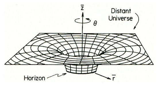
Figure 6.
On a flat manifold, two nearby geodesics that begin as parallel will remain parallel throughout their evolution. This, however, does not hold in the case of a curved manifold. In such a setting, geodesic deviation reflects the intrinsic curvature of the space, indicating that spacetime curvature and tidal forces are fundamentally the same phenomenon described in different terms.
A spacetime singularity denotes a failure in the manifold’s structure. All causal geodesics are terminated by generalized curvature singularities, which are categorized through the interplay between causal structure and curvature intensity. We consider the emergence of both local and global singularities in the brain as a curved Lorentzian manifold, originating from the collapse of a toroidal manifold dust cloud governed by Einstein–Maxwell dynamics with a non-zero velocity profile. In this framework, future-directed null geodesics exit the boundary of the synaptic activity cloud, whereas in the past, they converge to the singularity. Déjà vu may serve as an observable manifestation of such an effect. To preserve physical plausibility, the singularity must satisfy the conditions of a strong curvature singularity.
So, déjà vu may be reinterpreted from a geometric standpoint, specifically as a curvature spacetime singularity embedded in the global dynamics of the brain toroidal manifold. What occurs in the brain during such experiences? Neuroscientific research suggests that déjà vu is not indicative of a pathological condition, nor is it a failure of memory [67,68]. Despite this, no unified explanatory model has gained consensus. Nevertheless, a prevailing hypothesis posits that déjà vu arises when specific neural circuits interpret a current experience as resembling a past event, even in the absence of explicit recall. This suggests that the phenomenon may be rooted in memory processes, wherein the brain detects partial overlaps between present and previously encoded experiences. Einstein–Maxwell’s brain field equations lead to the formation of inherent curvature spacetime singularities; so, déjà vu could be an inherent process in synaptic dynamics.
4. Conclusions
Differential Geometry provides a powerful framework for identifying the shortest paths in metric spaces, with most path optimization problems naturally leading to the construction of a Lorentzian manifold. Furthermore, it offers significant geometric insights into the nature of these optimization problems. The approach presented in this work diverges from conventional methods, which typically solve path optimization problems by directly solving the equations of motion. Instead, this study formulates the problem geometrically and employs the tools of Differential Geometry to derive a solution.
The longstanding difficulties in achieving a unified and geometric description of the Einstein–Maxwell field theory suggest that their combination should be pursued directly at the level of the Lagrangian density. Moreover, simply adding the individual Lagrangians and imposing the coupling class within the Lagrangian (or equivalently, in the equations of motion) effectively constrains the trajectory as well. This requires adding a scalar field with appropriate units to restore the correct dimensions to the connection and to provide a kinetic term in the Lagrangian, which is necessary to ensure all fields are treated on equal terms. We applied the Lagrangian formulation to perform an extensive examination of the stability of geodesics around VNS toroidal manifold solutions to dynamical Einstein–Maxwell field theory, a theory that introduces modifications to General Relativity via a scalar field non-minimally coupled to curvature scalars.
The primary distinction of this method compared to traditional approaches is its ability to translate path stability problems into geometric manifolds. Moreover, the curvature and other geometric properties of these manifolds are intrinsic to the stability problems they represent, directly reflecting the underlying structure of the problem. We have established that metric (12) is free of singularities and fully consistent with the principal singularity theorems. Indeed, once the properties of the solution are understood, its singularity-free character becomes evident.
The formulation of electromagnetic field theory in curved spacetimes or from the perspective of accelerated observers reveals unexpected features of Maxwell’s theory that are not apparent in Minkowskiian spacetimes. More recently, it has been conjectured that changes in the topology of spacetime may further alter established results and provide new insights into their interpretation [69]. While modifications of the topology of the spatial sector alone have been extensively studied—showing that they primarily affect the spatial part of the positive and negative frequency mode bases of field solutions, as well as the vacuum energy (as in the Casimir effect)—global changes in the topology of both spatial and temporal sectors lead to more profound consequences. Notably, such topological modifications have been investigated in the contexts of black holes, de Sitter spacetime, and anti-de Sitter spacetime [70].
It is well established that singularity-free solutions are rare, especially when considering those with cosmological features. Here, we are not referring to solutions that can realistically describe the observed Universe (or brain synaptic activity in our case). This leads to the question of how many singularity-free solutions actually exist and what properties they should fulfil.
It may be argued, for instance, that the particular topology of the manifold (a torus) plays a role in the avoidance of singularities. In [71], a large family of singularity-free metrics for perfect fluids without any imposed equation of state was constructed, sharing similar features with our metric (12). All members of this family are cylindrically symmetric, and indeed, every other solution reported in [71] lacking this symmetry exhibits singularities. This suggests that cylindrical symmetry may be of some significance in the avoidance of singularities, although such a conclusion must, of course, be regarded only as a hypothesis.
The human brain’s structural network exhibits a rich and intricate topology, which researchers have extensively sought to characterize through conventional metrics and concepts from network science. Nonetheless, this characterization remains incomplete, as the subtler features of the topology continue to elude comprehensive and constructive modelling efforts. This study offers a framework for investigating the geometric complexity of the human structural connectome in the contexts of cognition, health, and disease.
Author Contributions
Conceptualization, M.R. (Manuel Rivas); Methodology, M.R. (Manuel Rivas); Formal analysis, M.R. (Manuel Rivas); Investigation, M.R. (Manuel Rivas) and M.R. (Manuel Reina); Writing—original draft, M.R. (Manuel Rivas) and M.R. (Manuel Reina); Writing—review & editing, M.R. (Manuel Reina); Project administration, M.R. (Manuel Reina). All authors have read and agreed to the published version of the manuscript.
Funding
This work was supported by research grants PID2023-148793NB-I00 and PID2023-149249NB-I00 and funded by MICIU/AEI/10.13039/501100011033, ‘ERDF—A way of making Europe’, and the Commission for Universities and Research of the Department of Innovation, Universities, and Enterprise of the Generalitat de Catalunya (SGR2021-00453).
Data Availability Statement
The original contributions presented in this study are included in the article. Further inquiries can be directed to the corresponding author.
Conflicts of Interest
The authors declare no conflict of interest.
References
- Gardner, R.J.; Hermansen, E.; Pachitariu, M.; Burak, Y.; Baas, N.A.; Dunn, B.A.; Moser, M.B.; Moser, E.I. Toroidal topology of the population activity in grid cells. Nature 2022, 602, 123–149. [Google Scholar] [CrossRef]
- Gastner, M.T.; Odor, G. The topology of large Open Connectome networks for the human brain. Sci. Rep. 2016, 6, 27249–27262. [Google Scholar] [CrossRef]
- Singh, G.; Memoli, F.; Ishkhanov, T.; Sapiro, G.; Carlsson, G.; Ringach, D.L. Topological analysis of population activity in visual cortex. J. Vis. 2008, 8, 11. [Google Scholar] [CrossRef]
- Rivas, M.; Reina, M. Covariant Formulation of the Brain’s Emerging Ohm’s Law. Symmetry 2024, 16, 1570. [Google Scholar]
- Xu, Y.; Long, X.; Feng, J.; Gong, P. Interacting spiral wave patterns underlie complex brain dynamics and are related to cognitive processing. Nat. Hum. Behav. 2023, 7, 1196–1215. [Google Scholar] [CrossRef]
- Rivas, M.; Reina, M. Riemannian topological analysis of neuronal activity. Symmetry 2025, 17, 412. [Google Scholar]
- Witten, L. (Ed.) A Geometric Theory of the Electromagnetic and Gravitational Fields, Gravitation an Introduction to Current Research; John Wiley & Sons, Inc: Hoboken, NJ, USA, 1962; pp. 45–48. [Google Scholar]
- Arfken, G.B.; Weber, H.J.; Harris, F.E. Mathematical Methods for Physicists; Addison-Wesley: San Francisco, CA, USA, 2013; pp. 134–156. [Google Scholar]
- Misner, C.W.; Wheeler, J.A. Classical physics as geometry: Gravitation, electromagnetism, unquantized charge, and mass as properties of curved empty space. Ann. Phys. 1957, 2, 525–603. [Google Scholar] [CrossRef]
- Carroll, S.M. Spacetime and Geometry: An Introduction to General Relativity; Addison-Wesley: San Francisco, CA, USA, 2004; p. 145. [Google Scholar]
- Rainich, G.Y. Electrodynamics in General Relativity. Trans. Amer. Math. Soc. 1925, 27, 106–119. [Google Scholar] [CrossRef]
- Stephani, H.; Kramer, D.; MacCallum, M.A.H.; Hoenselaers, C.; Herlt, E. Exact Solutions of Einstein’s Field Equations; Cambridge University Press: Cambridge, UK, 2003; pp. 56–59. [Google Scholar]
- Susskind, L.; Friedman, A. Special Relativity and Classical Field Theory: The Theoretical Minimum; Basic Books: New York, NY, USA, 2017; pp. 145–146. [Google Scholar]
- Wheeler, J.A. Problems on the frontiers between General Relativity, and Differential Geometry. Rev. Mod. Phys. 1962, 34, 873–879. [Google Scholar] [CrossRef]
- Thorne, C.M.; Thorne, K.S.; Wheeler, J.A. Gravitation; W H. Freeman and Company: San Francisco, CA, USA, 1971; p. 45. [Google Scholar]
- Hawking, S.W.; Ellis, G.F.R. The Large Scale Structure of Spacetime; Cambridge University Press: Cambridge, UK, 1973; p. 65. [Google Scholar]
- Eisenhart, L.P. Riemannian Geometry; Princeton University Press: Princeton, NJ, USA, 1964; p. 235. [Google Scholar]
- Romero, A.; Sánchez, M. On the completeness of geodesic obtained as limit. J. Math. Phys. 1993, 34, 3768–3774. [Google Scholar] [CrossRef]
- Hartle, J.B. Gravity: An Introduction to Einstein’s General Relativity; Addison-Wesley: San Francisco, CA, USA, 2003; p. 87. [Google Scholar]
- Adler, R.; Bazim, M.; Schiffer, M. Introduction to General Relativity; Mac Graw Hill: New York, NY, USA, 1965; pp. 65–68. [Google Scholar]
- Isham, C.J. Quantum Gravity, an Oxford Symposium; Clarendon Press: Oxford, UK, 1978; p. 500. [Google Scholar]
- Kuchasr, K. Relativity, Astrophysics and Cosmology. In Proceedings of the Summer School Held, Banff Centre, Banff, AB, Canada, 14–26 August 1972. [Google Scholar]
- Aldersey, S.J. Dimensional analysis in relativistic gravitational theories. Phys. Rev. D. 1977, 15, 370–376. [Google Scholar] [CrossRef]
- Lovelock, D. The four-dimensionality of space and the Einstein tensor. J. Math. Phys. 1972, 13, 874–876. [Google Scholar] [CrossRef]
- Lovelock, D. The uniqueness of the Einstein field equations in a four-dimensional space. Arch. Ration. Mech. Anal. 1969, 33, 54–70. [Google Scholar] [CrossRef]
- Moulin, F. Generalization of Einstein’s gravitational field equations. Eur. Phys. J. C 2017, 77, 878–892. [Google Scholar] [CrossRef]
- Radzikowski, M.J. Micro-local approach to the Hadamard condition in quantum field theory on curved space-time. Commun. Math. Phys. 1996, 179, 529–572. [Google Scholar] [CrossRef]
- Thomas, T.J. Differential Invariants of Generalized Spaces; Cambridge University Press: Cambridge, UK, 1934; p. 145. [Google Scholar]
- Noriega, R.J.; Schifini, C.G. Scalar density concomitants of a metric and a bivector. Gen. Relativ. Gravit. 1984, 16, 293–296. [Google Scholar] [CrossRef]
- Castagnino, M.; Domenech, G.; Levinas, M.; Umérez, N. Classical dynamical variables for the Wess-Zumino matter Lagrangian. Class. Quantum Grav. 1989, 6, 345–367. [Google Scholar]
- Nomizu, K.; Ozeki, H. The existence of complete Riemannian metrics. Proc. Amer. Math. Soc. 1961, 12, 889–891. [Google Scholar] [CrossRef]
- Coley, A.A.; Tupper, B.O.J. Special conformal Killing vector space-times and symmetry inheritance. J. Maths. Phys. 1989, 30, 2616–2625. [Google Scholar] [CrossRef]
- González, G.A.; Gutiérrez-Piñeres, A.C.; Ospina, P.A. Finite axisymmetric charged dust disks in conformastatic spacetimes. Phys. Rev. D Part. Fields Gravit. Cosmol. 2008, 78, 064058. [Google Scholar] [CrossRef][Green Version]
- Landsman, K. Penrose’s 1965 singularity theorem: From geodesic incompleteness to cosmic censorship Landsman, K. Gen. Relativ. Gravit. 2022, 54, 115. [Google Scholar] [CrossRef]
- Penrose, R. Quantum Theory and Beyond; Cambridge University Press: Cambridge, UK, 1972; p. 123. [Google Scholar]
- Yurtsever, U. A simple proof of geodesical completeness for compact space-times of zero curvature. J. Math. Phys. 1992, 33, 1295–1300. [Google Scholar] [CrossRef]
- Hawking, S.W. Properties of Expanding Universes. PhD Thesis, University of Cambridge, Cambridge, UK, 1965; p. 444. [Google Scholar]
- Misner, C.W.; Taub, A.H. A singularity-free empty universe. Sov. Phys. JETP. 1969, 55, 233–255. [Google Scholar]
- Penrose, R. Gravitational collapse. In Gravitational Radiation and Gravitational Collapse; DeWitt-Morette, C., Ed.; International Astronomical Union: Paris, France, 1974; pp. 82–91. [Google Scholar]
- Penrose, R. Gravitational collapse and space-time singularities. Phys. Rev. Lett. 1965, 14, 57–59. [Google Scholar] [CrossRef]
- Arnold, V.I. Ordinary Differential Equations; MIT Press: Cambridge, MA, USA, 1973; p. 76. [Google Scholar]
- Senovilla, J.M.M. New class of inhomogeneous cosmological perfect-fluid solutions without big-bang singularity. Phys. Rev. Lett. 1990, 64, 2219–2224. [Google Scholar] [CrossRef]
- Chinea, F.J.; Fernández-Jambrina, L.; Senovilla, J.M.M. Singularity-free space-time. Phys. Rev. D 1992, 45, 481–486. [Google Scholar] [CrossRef] [PubMed]
- Utiyama, R.; DeWitt, B.S. Renormalization of a classical gravitational field interacting with quantized matter fields. J. Math. Phys. 1962, 3, 608–615. [Google Scholar] [CrossRef]
- Kim, S.W.; Thorpe, K.S. Do vacuum fluctuations prevent the creation of closed timelike curves? Phys. Rev. D 1991, 43, 3929–3947. [Google Scholar] [CrossRef]
- Seifert, H.J. The causal boundary of space-times. Gen. Rel. Grav. 1971, 1, 247–259. [Google Scholar] [CrossRef]
- Ward, R.S.; Wells Jr, R.O. Twistor Geometry and Field Theory; Cambridge Monographs on Mathematical Physics; Cambridge University Press: Cambridge, UK, 1990; pp. 145–156. [Google Scholar]
- Goldman, W.; Hirsch, M. Affine manifolds and orbits of algebraic groups. Trans. Amer. Math. Soc. 1986, 295, 175–198. [Google Scholar] [CrossRef]
- Morris, M.S.; Thorne, K.S.; Yurtsever, U. Wormholes, time machines and the weak energy condition. Phys. Rev. Lett. 1988, 61, 1446–1449. [Google Scholar] [CrossRef]
- Waelbroek, H. Do universes with parallel cosmic strings or two-dimensional wormholes have closed timelike curves? Gen. Rel. Grav. 1991, 23, 219–233. [Google Scholar] [CrossRef]
- Hawking, S.W. The chronology protection conjecture. Phys. Rev. D 1992, 46, 603–611. [Google Scholar] [CrossRef]
- Friedman, J.; Morris, M.S.; Novikov, I.D.; Echevarría, F.; Klinkhammer, K.S.; Thorne, U.; Yurtsever, U. Cauchy problem in spacetimes with a closed timelike curve. Phys. Rev. D 1990, 42, 1915–1930. [Google Scholar] [CrossRef]
- Frolov, V.P.; Novikov, I.D. Physical effects in wormholes and time machines. Phys. Rev. D 1990, 42, 1057–1065. [Google Scholar] [CrossRef]
- Ramond, P. Field Theory: A Modern Primer; Benjamin/Cummings Pub. Co., Advanced Book Program: Reading, MA, USA, 1981; p. 156. [Google Scholar]
- Milnor, J. On the existence of a connection with curvature zero. Comment. Math. Helv. 1958, 32, 215–223. [Google Scholar]
- Yurtsever, U. Test fields on compact space-times. J. Math. Phys. 1990, 31, 3064–3078. [Google Scholar] [CrossRef]
- Sachs, R.K.; Wu, H. General Relativity for Mathematicians; Graduate Texts in Mathematics; Springer: New York, NY, USA, 1977; pp. 89–92. [Google Scholar]
- Marsden, J.E. On completeness of homogeneous pseudo-Riemann manifolds. Indiana Uni. Math. J. 1973, 22, 1065–1066. [Google Scholar] [CrossRef]
- Carrière, Y. Un survol de la théorie des variétés affines. Séminaire De Théorie Spectrale Et Géométrie 1987, 6, 9–22. [Google Scholar]
- Kobayashi, S.; Nomizu, K. Foundations of Differential Geometry; Wiley-Interscience: New York, NY, USA, 1963; Volume 1, p. 292. [Google Scholar]
- O’Neill, B. Semi-Riemannian Geometry with Applications to Relativity; Academic Press: New York, NY, USA, 1983; p. 43. [Google Scholar]
- Milnor, J. On fondamental groups of complete affinely flat manifolds. Adv. Math. 1977, 25, 178–187. [Google Scholar] [CrossRef]
- Farkas, H.M.; Kra, I. Riemann Surfaces; Graduate Texts in Mathematics; Springer: New York, NY, USA, 1992; p. 198. [Google Scholar]
- Kulkarni, R.S. An analogue to the Riemann mapping theorem for Lorentz metrics. Proc. R. Soc. Lond. 1985, 401, 117–130. [Google Scholar]
- Tipler, F.J. Causally symmetric spacetimes. J. Math. Phys. 1977, 18, 1568–1573. [Google Scholar] [CrossRef]
- Sullivan, D. A generalization of Milnor’s inequality concerning affine foliations and affine manifolds. Comm. Math. Helv. 1976, 51, 83–189. [Google Scholar] [CrossRef]
- Stendardi, D.; Basu, A.; Treves, A.; Ciaramelli, E. Déjà vu: A botched memory operation, illegitimate to start with. Behav. Brain Sci. 2023, 14, 46–58. [Google Scholar] [CrossRef]
- Spatt, J. Déjà vu: Possible parahippocampal mechanisms. J. Neuropsychiatry Clin. Neurosci. 2002, 14, 6–10. [Google Scholar] [CrossRef]
- Low, R.J. The geometry of the space of null geodesics. J. Math. Phys. 1989, 30, 809–811. [Google Scholar] [CrossRef]
- Hackmann, E.; Lämmerzahl, C. Geodesic equation in Schwarzschild-(anti)- de Sitter space-times: Analytical solutions and applications. Phys. Rev. D Part. Fields Gravit. Cosmol. 2008, 78, 1–22. [Google Scholar] [CrossRef]
- Ruiz, E.; Senovilla, J.M.M. General class of inhomogeneous perfect-fluid solutions. Phys. Rev. D 1992, 45, 1995–2005. [Google Scholar] [CrossRef]
Disclaimer/Publisher’s Note: The statements, opinions and data contained in all publications are solely those of the individual author(s) and contributor(s) and not of MDPI and/or the editor(s). MDPI and/or the editor(s) disclaim responsibility for any injury to people or property resulting from any ideas, methods, instructions or products referred to in the content. |
© 2025 by the authors. Licensee MDPI, Basel, Switzerland. This article is an open access article distributed under the terms and conditions of the Creative Commons Attribution (CC BY) license (https://creativecommons.org/licenses/by/4.0/).