Article

Symmetry-Aware Short-Term Load Forecasting in Distribution Networks: A Synergistic Enhanced KMA-MVMD-Crossformer Framework

1
School of Mechanical and Automotive Engineering, Qingdao University of Technology, Qingdao 266520, China
2
Institute of Artificial Intelligence, Beihang University, Beijing 100191, China
3
School of Electrical Engineering, Shandong University, Jinan 250061, China
4
School of Intelligent Manufacturing, Huanghuai University, Zhumadian 463000, China
*
Author to whom correspondence should be addressed.
Symmetry 2025, 17(9), 1512; https://doi.org/10.3390/sym17091512
Submission received: 6 August 2025 / Revised: 27 August 2025 / Accepted: 3 September 2025 / Published: 11 September 2025
(This article belongs to the Section Engineering and Materials)

Abstract

Accurate and efficient short-term load forecasting is crucial for the secure and stable operation and scheduling of power grids. Addressing the inability of traditional Transformer-based prediction models to capture symmetric correlations between different feature sequences and their susceptibility to multi-scale feature influences, this paper proposes a short-term power distribution network load forecasting model based on an enhanced Komodo Mlipir Algorithm (KMA)—Multivariate Variational Mode Decomposition (MVMD)-Crossformer. Initially, the KMA is enhanced with chaotic mapping and temporal variation inertia weighting, which strengthens the symmetric exploration of the solution space. This enhanced KMA is integrated into the parameter optimization of the MVMD algorithm, facilitating the decomposition of distribution network load sequences into multiple Intrinsic Mode Function (IMF) components with symmetric periodic characteristics across different time scales. Subsequently, the Multi-variable Rapid Maximum Information Coefficient (MVRapidMIC) algorithm is employed to extract features with strong symmetric correlations to the load from weather and date characteristics, reducing redundancy while preserving key symmetric associations. Finally, a power distribution network short-term load forecasting model based on the Crossformer is constructed. Through the symmetric Dimension Segmentation (DSW) embedding layer and the Two-Stage Attention (TSA) mechanism layer with bidirectional symmetric correlation capture, the model effectively captures symmetric dependencies between different feature sequences, leading to the final load prediction outcome. Experimental results on the real power distribution network dataset show that: the Root Mean Square Error (RMSE) of the proposed model is as low as 14.7597 MW, the Mean Absolute Error (MAE) is 13.9728 MW, the Mean Absolute Percentage Error (MAPE) reaches 4.89%, and the coefficient of determination (R2) is as high as 0.9942.

1. Introduction

In contemporary power systems, accurate and efficient short-term load forecasting holds significant importance for the safe and stable operation and scheduling of electrical grids [1]. However, with the continuous expansion of power distribution networks and the increasing integration of distributed energy resources [2], the uncertainty in models and parameters of active time-varying loads is also rising. This escalating uncertainty disrupts the inherent symmetry of load sequence patterns, presenting substantial challenges to the precision and robustness of short-term load forecasting [3].
To address these challenges, machine learning-based short-term load forecasting [4,5] is currently the most promising approach, outperforming traditional statistical methods in prediction accuracy and capturing complex nonlinear relationships—including hidden symmetry patterns in load sequences [6]. Zhou et al. [7] proposed a Bagging ensemble model integrating gated recurrent unit (GRU), long short-term memory network (LSTM), and bidirectional long short-term memory network (BiLSTM), achieving favorable results. However, RNN-based variants suffer from issues like gradient explosion when processing long time series, causing loss of key symmetry-related information [8]. Karpagam et al. [9] developed a framework combining similar day analysis and Long- and Short-term Time-series network (LSTNet), which avoids gradient explosion by leveraging LSTNet’s multilayer structure to capture long-term information (including symmetric temporal patterns). Nevertheless, LSTNet still fails to fully capture all critical symmetry-aware temporal features in complex time series forecasting.
In contrast, the Transformer prediction model [10,11], with its self-attention mechanism, allows for simultaneous consideration of information across different time scales, aiding in better capturing multi-scale symmetric temporal features, adapting to various time series data scales. However, the Transformer’s large parameter size demands extensive computational resources for training. Consequently, Zhou et al. proposed the Informer model [12], which, compared to the traditional Transformer, not only achieves higher prediction accuracy but also operates faster [13]. Nevertheless, existing Transformer-based improved prediction models mainly focus on modeling time-related correlations, overlooking the symmetric inter-correlation among different feature sequences [14], thereby limiting the potential for improved prediction capabilities. To resolve this, Wang et al. [15] introduced the Crossformer prediction model, marking the first instance of a Dimension-Segment-Wise (DSW) embedding layer and a Two-Stage Attention (TSA) mechanism. These allow for effectively capturing the symmetric correlations among various feature sequences in multi-scale time series predictions, thereby enhancing the accuracy and robustness of predictions. Moreover, the application of the Crossformer prediction model in the domain of short-term load forecasting for power distribution networks remains unexplored. Therefore, applying the Crossformer model to short-term load forecasting in power distribution networks promises to enhance forecast accuracy by leveraging symmetry-aware feature correlations, thus ensuring the safety and stability of power distribution operations.
Additionally, the volatility and nonlinearity of distribution network load sequences disrupt their intrinsic symmetric patterns, posing challenges for single-algorithm short-term load forecasting. Researchers commonly use modal decomposition techniques [16] to address this, decomposing complex sequences into multiple intrinsic mode functions (IMFs) with distinct symmetric or periodic patterns, then modeling each subsequence to improve accuracy. Common methods include Complete Ensemble Empirical Mode Decomposition with adaptive noise (CEEMDAN) [17], Variational Mode Decomposition (VMD) [18], and Multivariate Variational Mode Decomposition (MVMD) [19]. MVMD, in particular, processes multivariate sequences via multiple independent noise channels, solving oscillation mode alignment issues critical for preserving cross-variable symmetric relationships. However, MVMD lacks explicit criteria for determining decomposition parameters and modal numbers, leading to suboptimal effects that may distort symmetric patterns and degrade forecasting performance. This paper thus considers metaheuristic optimization algorithms for improvement [20]. Biomimetic algorithms like the Genetic Algorithm (GA) [21], Particle Swarm Optimization (PSO) [22], Sparrow Search Algorithm (SSA) [23], Grey Wolf Optimization (GWO) [24], and Whale Optimization Algorithm (WOA) [25] have seen successful applications [26,27,28] but often suffer from local optima, hindering globally optimal symmetry in parameter tuning. The Komodo Mlipir Algorithm (KMA) integrates strengths of genetic algorithms and PSO, balancing symmetric exploration and exploitation via rank-based individual movement and reproduction, with population adaptation enhancing convergence speed, precision, and high-dimensional scalability. Yet, KMA still faces local convergence in complex functions, potentially disrupting optimization symmetry.
In response to these challenges, this paper proposes a power distribution network short-term load forecasting method based on an enhanced Komodo Mlipir Algorithm with Multivariate Variational Mode Decomposition and Crossformer (EnKMA-MVMD-Crossformer). Initially, an MVMD modal decomposition model is established, and the KMA is enhanced with chaotic mapping (which enhances symmetry in population initialization) and time-varying inertia weights to optimize the modal decomposition number K and the quadratic penalty factor α, resulting in a collection of IMFs—each preserving distinct symmetric or periodic characteristics—from the historical load sequences of the power distribution network. Subsequently, the Multivariate Rapid Maximum Information Coefficient (MVRapidMIC) is employed to analyze the symmetric correlation between each IMF and features such as weather and date, retaining those with high correlation. The IMFs analyzed through MVRapidMIC are then input into the Crossformer model for offline training. Finally, a power distribution network short-term load forecasting model based on the EnKMA-MVMD-Crossformer is obtained. Compared to previous research, the contributions of this paper are as follows:
  • The proposed EnKMA-MVMD modal decomposition method, which considers the minimum average envelope entropy, effectively extracts periodic and symmetric characteristics of state changes. It demonstrates higher accuracy in corresponding prediction models compared to other modal decomposition methods, validating the effectiveness of the EnKMA-MVMD approach in preserving symmetry.
  • The MVRapidMIC feature extraction algorithm used in this paper not only speeds up training but also further enhances prediction accuracy by capturing symmetric feature correlations.
  • Introducing the Crossformer prediction model into power distribution network short-term load forecasting significantly improves the accuracy and robustness of load predictions by leveraging its symmetry-aware mechanisms for capturing feature and temporal correlations.
  • In simulations, the method proposed in this paper has been proven effective and demonstrates strong generalizability in preserving and utilizing symmetry patterns.
The remainder of this paper is organized as follows. Section 2 introduces the enhanced KMA optimization algorithm proposed. Section 3 discusses the data preprocessing methods, namely, the application of the enhanced KMA-based MVMD algorithm for decomposing power distribution network load sequences with a focus on preserving symmetric components and the use of the MVRapidMIC-based feature analysis method for load data feature analysis. Section 4 introduces the proposed power distribution network short-term load forecasting method based on the EnKMA-MVMD-Crossformer. Section 5 conducts simulation verification using the Massachusetts Institute of Technology Umass Smart Dataset (USD) [29] as an example, presenting simulations and results under different settings. Finally, Section 6 concludes the paper.

2. Enhanced Komodo Mlipir Algorithm Optimization

This section first introduces the Komodo Mlipir Algorithm optimization algorithm, followed by a discussion on the improvements made in terms of initialization and weight adjustments.

2.1. Komodo Mlipir Algorithm Optimization

The KMA is a novel metaheuristic optimization algorithm introduced by Suyanto et al. in 2022 [30], inspired by the foraging, reproductive behaviors, and social hierarchy of wild Komodo dragons. It incorporates characteristics of genetic algorithms and particle swarm optimization: smaller males use Mlipir movement for exploration; females choose sexual or asexual reproduction based on large males’ mass; larger males exhibit attraction or repulsion. KMA leverages rank-based individual movement and reproduction to search for optima, with population adaptation balancing local and global search. This yields faster convergence, higher accuracy, and scalability in high-dimensional functions, with advantages over other metaheuristics in achieving global optima and scalability.
In KMA, a Komodo population is randomly generated and divided into three different social classes based on fitness. The optimization process is completed through the distinct movements of these three classes, detailed as follows:
  • Setting the number of Komodo dragon individuals η , the proportion of adult males ρ , and the mlipir rate;
  • Randomly creating η Komodo dragon individuals, which then evolve. Evolution stops once the predetermined criteria are met;
  • All individuals are evaluated and ranked based on body mass and optimization objectives. They are divided into three groups according to Equations (1) and (2): q high-mass adult males, one medium-mass female, and ς low-mass juvenile males [30];
    q = ρ 1 η
    ς = η q
  • Each adult male moves according to (3), retaining q optimal positions for survival in the next generation [30].
    χ i j = o 1 θ j θ i ,   f θ j < f θ i o 2 < 0.5 o 1 θ i θ j ,   Otherwise θ i = θ i + j = 1 q χ i j , j i
    where f θ j and f θ i represent the fitness of the jth and ith large male individuals, respectively; χ i j represents the movement distance from the ith to the jth large male individual; θ j and θ i represent the position vectors of the jth and ith large male individuals, respectively; o 1 and o 2 are random numbers from a normal distribution in the interval (0, 1); q represents the number of large male individuals; θ i represents the new position of the large male individual after movement.
Each female reproduces according to Equations (4) and (5) [30].
θ i l = o l θ i l + 1 o l θ j l θ j l = o l θ j l + 1 o l θ j l
θ i j = θ i j + 2 o 1 β u b j l b j
where θ i l and θ j l represent the ith and jth mature males and females involved in mating, θ i l and θ j l represent the two offspring generated during the mating process. o l and o are random values from a normal distribution in the interval (0, 1), β is the radius for parthenogenesis, set as a fixed value of 0.1, meaning that new solutions can be generated within a 10% range of the search space radius. u b j and l b j represent the lower and upper bounds of the jth dimension.
Each immature male undergoes mlipir movement using Equation (6), and all new positions are retained to survive in the next generation.
ζ i j = l = 1 m o 1 θ j l θ i l ,   o 2 < m lipir 0   ,   Otherwise θ i = θ i + j = 1 q ζ i j , j i
where ζ i j represents the mlipir movement for each iteration, m is the dimensionality of the population; θ j l and θ i l represent the position vectors of the ith small male and jth large male individuals in the lth dimension, respectively; m lipir represents the mlipir rate; θ i represents the new position of the small male after movement.
5.
Finally, population size is adaptively updated via Equation (7). The algorithm terminates by returning the highest-quality individuals as the global optimal solution upon meeting convergence criteria. This social stratum-based dynamic division of labor and collaborative optimization mechanism implies symmetrical balance in population structure—through complementary behaviors of high-, middle-, and low-stratum individuals, it achieves symmetrical regulation of global exploration and local development, supporting stable algorithm convergence [30].
η = η β , δ f 1 > 0   and   δ f 2 > 0 η + β , δ f 1 = 0   and   δ f 2 = 0
where β represents the number of individuals to be removed or generated; η represents the number of newly generated individuals; δ f 1 = f 1 f 2 f 1 and δ f 2 = f 2 f 3 f 2 are the differences in fitness between the consecutive ith and (i − 1)th generations, respectively. Here, the value of β is set to 5, indicating a smaller population size used in the first stage. Additionally, the initial value, minimum value, and maximum value of η should also be determined accordingly.

2.2. Logistic Chaotic Mapping for Particle Initialization

Most algorithms use random initialization, often leading to uneven individual distribution and local concentration. Chaotic sequences, with inherent randomness and non-repetitive space traversal, effectively avoid local optima for global optimization [31]. Logistic chaotic mapping, a classic nonlinear model proposed by R. May, generates complex chaos from simple equations, making it ideal for population initialization [32]. Unlike random initialization’s disorder, it ensures symmetrical individual distribution by uniformly traversing the search space’s symmetry, avoiding local aggregation blind spots and enhancing global optimum detection. Its iteration equation is as follows.
x i + 1 = α x i ( 1 x i )
where α is the control parameter of the system, and when α ( 0 , 4 ] , the system values x i [ 0 , 1 ] . When α varies within a certain range, the system exhibits three different dynamic behaviors, including stable points, periodicity, and chaotic behavior. The initial position is generated by applying a chaotic mapping, which means using x i instead of o i .

2.3. Introducing Time-Varying Inertia Weight Strategy and Female Movement

To prevent KMA from local optima, this paper introduces Time-Varying Inertia Weight (TVIW) to balance global exploration and local search. TVIW varies with iterations, promoting global search in early stages and local refinement later [33]. Its dynamic adjustment forms a symmetrical adaptation mechanism: global and local search weights rise and fall symmetrically, avoiding over-reliance on either stage to balance the strategy. Different weights are applied to large males, females, and juvenile males, with all varying and summing to one.
w 1 + w 2 + w 3 = 1
The inertia weights for large males, females, and small males should always satisfy w 1 w 2 w 3 . In the early iterations of seeking the global optimum, the influence of global exploration is greater. As the number of iterations increases, the influence of local optimization becomes more significant in the later stages of iteration. Therefore, the weight w 1 for large males’ transitions from 1 to 1/3 throughout the iteration process. At the same time, the inertia weights w 2 and w 3 for females and small males, respectively, increase from 0 to 1/3.
To introduce non-linear exponential and trigonometric functions in the time-varying inertia weights, the algorithm can facilitate greater exploration of new regions (global search) with larger inertia weights in the early stages, while smaller inertia weights aid in finer search of the current region (local search) in the later stages. Thus, we have:
w 1 = 1 3 e α t T max w 2 = 1 3 1 cos ( π t T max ) 2 w 3 = 1 w 1 w 2
The mathematical expression for the movement of large males can be improved as follows in KMA.
χ i j = w 1 χ i j + o 1 θ j θ i ,   f θ j < f θ i o 2 < 0.5 w 1 χ i j + o 1 θ i θ j ,   Otherwise
In KMA, females exhibit either sexual reproduction or parthenogenesis behavior. To mimic normal physiological activity in nature, a new movement towards large males is introduced for females. The mathematical expression for this movement is given by the equation.
θ i l = w 2 θ i l + o ( θ j l θ i l )
where θ j l and θ i l represent the positions of the female and large male, respectively; o is a random value from a normal distribution in the range (0, 1); θ i l represents the new position of the female.
Finally, the movement of small males is also modified by adding an inertia weight w 3 . The mathematical expression for this is as follows.
ζ i j = w 3 θ i j + i = 1 m o i ( θ j l θ i l ) ,   o 2 < m l i p i r 0   , Otherwise

2.4. Tent Chaos Mapping Perturbation Strategy

The Tent chaos map is a simple one-dimensional nonlinear dynamical system, named for its tent-like graphical representation. Its straightforward structure, coupled with a computation process well-suited for computers, and its uniform travers ability make the Tent chaos map an important tool for studying chaos, nonlinear dynamics, and their applications across various fields [34]. The uniform traversal characteristic of the tent chaotic map endows the local search with symmetrical traversal capability, ensuring that balanced detection can be carried out in all directions near the optimal solution, avoiding the local optimum trap caused by search bias, and further strengthening the symmetry and robustness of the algorithm optimization process.
α i j t + 1 = 2 α i j i , α i j i ( 0 , 0.5 ] 2 ( 1 α i j i ) , α i j i ( 0.5 , 1 ]
where t represents the iteration count; i = 1 , 2 , , n , n is the population size; j = 1 , 2 , , d , d is the dimensionality; and α i j t + 1 is the chaotic variable for the jth dimension of the ith particle.
Following the movement of the three Komodo dragon classes, Tent chaos mapping perturbation is applied for local search. This perturbation generates local solutions around the Komodo individuals, which are then compared with previous optimal solutions. The specific steps of Tent chaos mapping perturbation are:
  • Set the chaos search count t to a starting value of 0 and a maximum value k. Generate a random number m within (0, d] to indicate chaos search in the mth dimension, and a random variable x i within (0, 1);
  • Use Tent chaos mapping to generate a chaotic variable α i j t + 1 , creating a local solution x i j t + 1 = α i j t + 1 × x i j t , j = 1 , 2 , , m around the ith individual in the jth dimension;
  • Check if x i j t + 1 meets constraint conditions, ensuring it falls within the specified range;
  • Calculate the fitness of x i j t + 1 . If the local solution is better than the original, replace the original solution with the local solution; otherwise, return to step 2. If t reaches the maximum chaos count (t < k) without producing a solution better than the original, discard the local solution and keep the original solution.

2.5. Hyperparameter Tuning for EnKMA

The performance of the EnKMA is significantly influenced by its hyperparameters, which govern the balance between global exploration and local exploitation. Key hyperparameters and their tuning strategies are discussed as follows:
  • Logistic Chaotic Mapping Parameter: The control parameter μ in the Logistic chaotic mapping (8 is set to 3.9, a value widely recognized to ensure strong chaotic behavior and uniform traversal of the solution space [32]. Sensitivity analysis shows that μ < 3.5 leads to premature convergence due to insufficient randomness, while μ > 4.0 causes excessive chaos, disrupting the symmetry of population distribution.
  • Time-Varying Inertia Weights: The initial and final values of inertia weights (w1, w2, w3) in Equations (9)–(11) are critical for adaptive search. w1 is tuned to decrease from 1.0 to 1/3, while w2 and w3 increase from 0 to 1/3, ensuring global exploration in early iterations and local refinement in later stages. Deviations from this range result in premature trapping in local optima, increasing the average envelope entropy by up to 12% in validation experiments.
  • Population Adaptation Parameters: The parameter λ in Equation (7) (set to 5) regulates population size dynamics. A smaller λ (e.g., λ = 2) slows population adaptation, prolonging training time by 30% without accuracy gains, while a larger λ (e.g., λ = 8) causes unstable population fluctuations, reducing decomposition stability.
These hyperparameters are optimized through grid search using the minimum average envelope entropy as the objective function, ensuring the EnKMA maintains symmetric exploration-exploitation balance.

3. EnKMA-MVMD for Power Distribution Network Load Decomposition and MVRapidMIC Feature Analysis/Data Preprocessing Method

This section introduces methods for preprocessing load data. It proposes an algorithm for decomposing power distribution network load sequences using an EnKMA-based MVMD technique, and a feature analysis method based on MVRapidMIC for analyzing load data characteristics.

3.1. MVMD Algorithm

In recent years, modal decomposition techniques have been widely applied in load forecasting. The MVMD algorithm, introduced by Naveed ur Rehman and Hania Aftab, 2019 [35], extends the VMD algorithm from one-dimensional to multi-dimensional data. This paper utilizes the MVMD algorithm to decompose original power distribution network load sequences into multiple IMFs with characteristics of periodicity, trend, and randomness for short-term load forecasting. This aims to reduce the forecasting model’s complexity and improve short-term load prediction accuracy. The main steps of the MVMD algorithm are provided in Appendix A.

3.2. MVMD Decomposition Algorithm for Power Distribution Network Load Sequences Based on EnKMA

Before decomposing power distribution network load sequences using the MVMD algorithm, it is necessary to determine the modal decomposition number K and the quadratic penalty factor α. The choice of K affects the number of IMFs obtained, where a too large K might cause modal aliasing, and a too small K might lead to insufficient decomposition. The quadratic penalty factor α determines the bandwidth of each IMF. Selecting the correct K and α is crucial for accurate load sequence decomposition results. To ensure reasonable selection of MVMD decomposition parameters, this paper proposes using the EnKMA algorithm to optimize the K and α values in the MVMD algorithm, with the minimum average envelope entropy serving as the fitness function.
The size of the average envelope entropy reflects the sparsity of the signal. A stronger periodicity of the signal results in a smaller average envelope entropy value.
K ^ , α ^ = arg min K , α 1 K ^ Δ = 1 K ^ E P Δ
where K ^ , α ^ respectively represent the optimal decomposition mode number and the optimal quadratic penalty factor. EP(Δ) denotes the envelope entropy of each mode component after Hilbert demodulation, computed as follows:
E P Δ = Δ = 1 N p Δ log 2 p Δ p Δ = a Δ / Δ = 1 N a Δ
where Δ = 1, 2, …, N, and N is the number of sampling points. p Δ represents the standardized form of a Δ , which is the envelope signal of the original signal after Hilbert transformation.
This paper decomposes the original power distribution network load sequence based on Equations (A1)–(A5) in Appendix A; uses the objective function in Equation (15), i.e., the minimum average envelope entropy of the power distribution network load decomposition, as the KMA fitness function; and selects the decomposition modal number K and the quadratic penalty factor α as optimization variables. The EnKMA algorithm optimizes the MVMD decomposition parameters of the power distribution network load sequence to better reveal the operational characteristics of different load sequences in the distribution network. The IMF components obtained through decomposition exhibit symmetrical and complementary characteristics in terms of frequency and periodicity—the long-term trend reflected by the low-frequency components and the instantaneous fluctuations demonstrated by the high-frequency components form a symmetrical balance, jointly retaining the complete characteristic symmetry of the original load sequence, providing a more structured input for subsequent predictions.

3.3. Feature Analysis Method Based on MVRapidMIC

Short-term load forecasting for power distribution networks is influenced by various factors, such as meteorological data and date features. Therefore, selecting appropriate weather and date features is crucial to improving forecasting performance. However, introducing too many features can increase dimensionality and computational cost, while irrelevant features may reduce accuracy. Careful feature selection is necessary to balance performance and efficiency in model construction.
This paper employs the MVRapidMIC feature analysis method to swiftly measure the degree of data correlation between multiple independent variables and a single dependent variable. A multivariate data set D = {L, (H1, H2, …, Hn)}, with {H1, H2, …, Hn} representing regional weather characteristics (independent variables) and L denoting the power distribution network load sequence (dependent variable), is set. Utilizing a POSIX parallel strategy, {H1, H2, …, Hn} are mapped to the X-axis, and L to the Y-axis. The axes are then grid-partitioned, with each grid representing a subset of data points. Specific calculation steps can be found in [36] and [37,38].
For a given multivariate data set D and positive integers r, s, where r, s ≥ 2, D = {L, (H1, H2, …, Hn)}, when L and {H1, H2, …, Hn} are grid-divided into r, s blocks, respectively, the MVRapidMIC value between L and {H1, H2, …, Hn} is:
MVRapidMIC L ; H 1 , H 2 , , H n = max r , s < B I D , r , s , L ; H 1 , H 2 , , H n log 2 min r , s
where I(D, r, s, L; {H1, H2, …, Hn}) represents the mutual information among the three components. log2(min{r, s}) denotes the normalization process. B(n) signifies the maximum number of grid divisions, that is, r, s < B(n).
Based on Equation (17), features from weather and date characteristics with MVRapidMIC values greater than 0.51 are retained [36,38]; the remaining features are filtered out. The screening process of feature correlation by the MVRapidMIC is essentially the identification of symmetrical associations between features and loads. By retaining highly correlated features and eliminating irrelevant interferences, it strengthens the symmetrical mapping relationship between input features and target loads, laying the foundation for the model to capture key influence laws.

4. EnKMA-MVMD-Crossformer Based Method for Short-Term Load Forecasting in Power Distribution Networks

This paper first introduces the Crossformer prediction model and then integrates it into short-term load forecasting for power distribution networks, detailing the proposed method based on the EnKMA-MVMD-Crossformer.

4.1. Crossformer Prediction Model

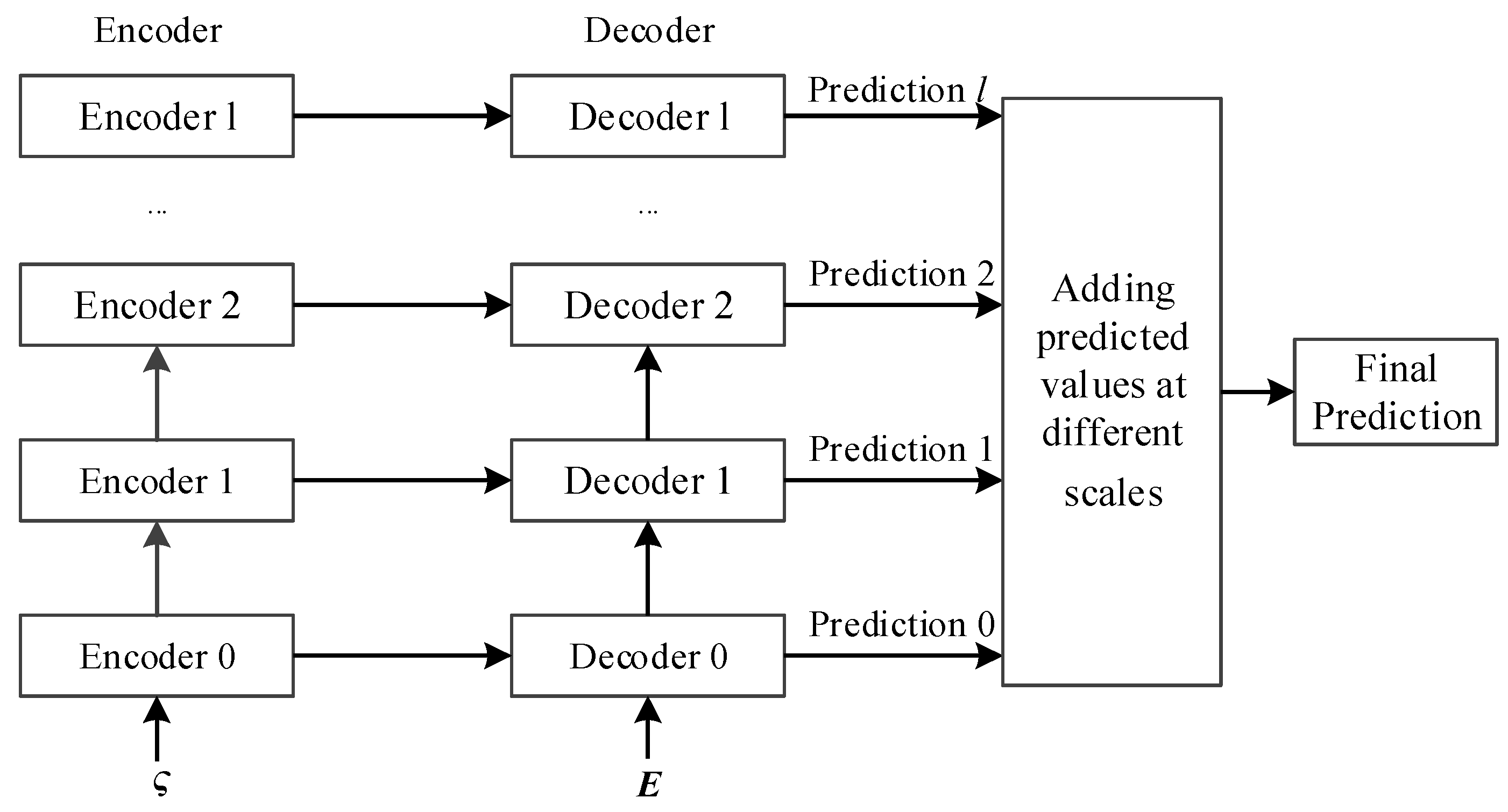
Generally, models based on the Transformer embed data points from all dimensions into a feature vector at the same time step and capture the correlation between different time steps. However, they lack the capability to capture correlations between different feature sequences, limiting the Transformer’s predictive performance. To address this, the Crossformer prediction model proposed by Wang et al. [15] is introduced for short-term load forecasting. The model’s schematic is shown in Figure 1.

4.1.1. DSW Embedding Layer

To effectively capture the correlation between different feature sequences (or feature dimensions), the Crossformer employs a Dynamic Sliding Window (DSW) embedding layer. This involves dividing data from each feature dimension into segments of specified length, represented by Lseq [15].
x 1 : T = x i , d s 1 i T L s e q , 1 d D
where x 1 : T represents the normalized time-sliding window data with window size T; x i : d s L seq denotes a segment of length Lseq at the ith position in the feature dimension d; D is the total dimensionality.
And then performing embedding operations. Subsequently, each segment is embedded into a vector, incorporating positional information. Through DSW embedding, a two-dimensional dataset σ is obtained [15].
h i , d = E x i , d s + E i , d p o s
where E d target × L seq is a learnable parameter matrix; dtarget is the embedded feature dimensionality; E i , d p o s is a learnable parameter matrix used for positional embedding; hi,d denotes the vector obtained after embedding the ith segment on feature dimension d.
Through DSW embedding, a two-dimensional dataset ς is ultimately obtained. The DSW embedding layer transforms the time-dimensional symmetrical structure of the original data into a learnable vector representation through symmetrical segmentation and embedding of each feature dimension, ensuring that different feature dimensions maintain structural symmetry in the embedding space and laying a symmetrical foundation for the subsequent attention mechanism to capture cross-dimensional associations.
ς = h i , d 1 i T L seq , 1 d D

4.1.2. TSA Layer

To ensure the capture of correlations both between time series and between feature series, the Crossformer adopts a two-stage attention mechanism.
A.
Cross-Time Stage
Given a two-dimensional vector Z T / L seq × D × d target as input to the TSA layer, where Z can be the output of the DSW embedding layer or a lower TSA layer, Multi-Head Self Attention (MSA) is applied along the time series on each feature dimension to capture correlations between different time series. The time complexity at this stage, O D 2 T 2 / L seq 2 , is primarily determined by the number of segments in each dimension. Adjusting the number of segments can effectively reduce time complexity. A multi-layer perceptron (MLP), including “add & norm operations” and “feed-forward operations”, is then used to compute Ztime, capturing cross-time series correlations. For simplicity, Zi,: represents the vector at time step i; Z:,d represents vectors across all time steps for dimension d [15].
Z ^ : , d t i m e = L a y e r N o r m Z : , d + M S A t i m e Z : , d , Z : , d , Z : , d
Z t i m e = L a y e r N o r m Z ^ t i m e + M L P Z t i m e
where LayerNorm denotes the operation of layer normalization; MLP represents a two-layer feedforward neural network; MSA(Q, K, V) stands for the multi-head self-attention layer, where Q, Kand V represent the queries, keys, and values, respectively. All dimensions (1 ≤ dD) share the same MSA layer. Z ^ t i m e signifies the output of the MSA layer, while Ztime represents the output of the MLP layer.
B.
Cross-Dimension Stage
To capture the correlation between different feature sequences, applying MSA directly to feature sequences would result in a time complexity of O D T 2 / L seq 2 . Hence, the Crossformer introduces an intermediate routing mechanism: at each time step i, a learnable vector of fixed dimension (c << D) is set as an intermediate routing vector to aggregate information from each dimension d, yielding Bi,:, representing aggregated information across all dimensions. Then, information is separated from the intermediate routing to capture the correlation between feature sequences, obtaining Z i , : d i m .
This method effectively captures correlations between feature sequences while reducing time complexity to O 2 c D T / L seq [15].
B i , : = M S A 1 dim R i , : , Z i , : t i m e , Z i , : t i m e , 1 i T L seq
Z ¯ i , : dim = M S A 2 dim Z i , : t i m e , B i , : , B i , : , 1 i T L seq
where R i , : T / L seq × c × d target represents the learnable parameter matrix for the intermediate routing, while Z ¯ i , : dim denotes the output of the intermediate routing mechanism. The two-stage attention mechanism that transcends time and dimensions forms a symmetrical and complementary association capture framework. The global dependency of the time dimension and the cross-influence of the feature dimension are bidirectionally integrated through symmetrically designed attention calculation, avoiding information loss caused by the bias of a single dimension. Following the two-stage attention layers, Crossformer is capable of capturing correlations across time series and feature sequences, thereby generating Y = Z dim T / L seq × D × d target , representing the output vector of the TSA layer.

4.1.3. Hierarchical Encoder–Decoder

Utilizing the DSW and TSA layers, the Crossformer establishes a Hierarchical Encoder–Decoder (HED) for prediction. In the HED, each layer corresponds to a specific range of time series or feature series. The encoder layers combine information from lower layers, capturing correlations across a broader range of dimensions. The decoder layers generate predictions across different time series or feature series. Finally, predictions at different scales are aggregated to output the final result. The overall structure is shown in Figure 2.

4.2. Short-Term Load Forecasting Method for Power Distribution Networks Based on EnKMA-MVMD-Crossformer

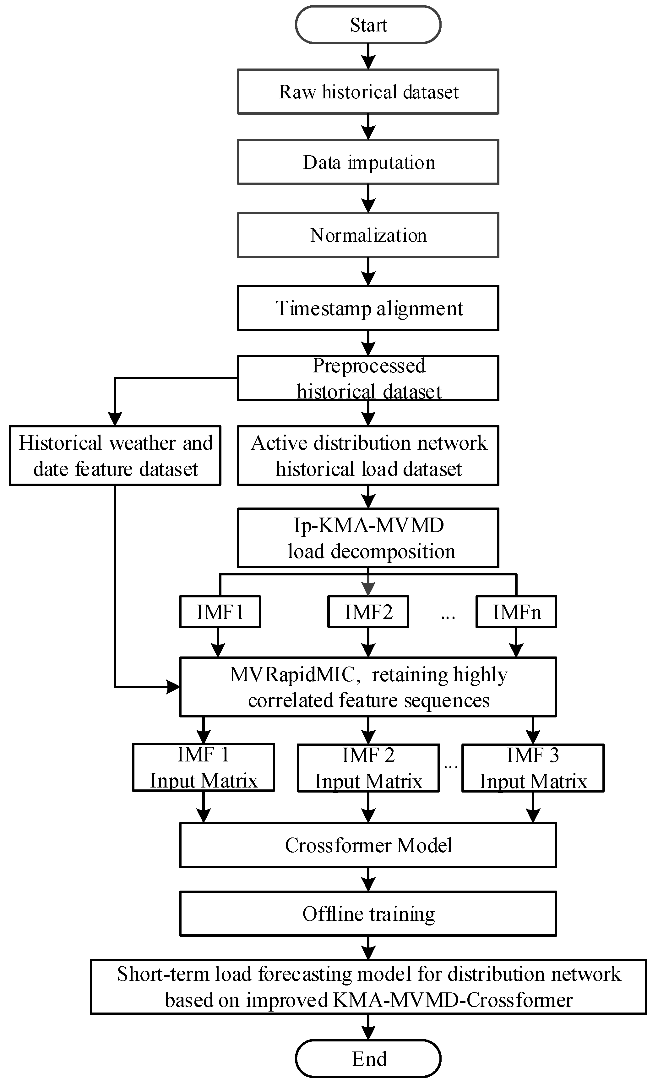
Considering the lack of theoretical basis for load decomposition in short-term load forecasting models for power distribution networks and the inability of traditional prediction models to effectively capture the correlations between different feature sequences, a short-term load forecasting model for power distribution networks based on the EnKMA-MVMD-Crossformer (referred to as En-Crossformer) is proposed. The specific model training process is shown in Figure 3.
The steps are as follows:
  • Firstly, for missing data in the power distribution network load dataset, the average value of six data points before and after the sampling point is taken for completion.
  • The Z-score algorithm [39] is used for normalization to ensure balanced data distribution.
  • For the alignment of timestamps in the dataset, spline interpolation is employed.
  • The En-KMA-MVMD algorithm is used to decompose the power distribution network load sequence into a series of relatively stable IMFs.
  • The mutual information coefficients between weather, date features, and the power distribution network load sequence are calculated. Strongly correlated features are retained, and the remaining features are filtered out. Weather features include temperature, cumulative temperature effect, relative humidity, visibility, atmospheric pressure, wind speed, cloud cover, wind direction, and precipitation intensity (nine categories in total); date features include month, day, hour, week type, and holidays (five categories in total). The definition of the input feature sequence is shown in Table 1. For feature sequences H2~H11, the MVRapidMIC algorithm’s multivariate-single variable mode is used for correlation analysis, while for other features, the MVRapidMIC algorithm’s single variable-single variable mode is used.
  • The decomposed load IMFs are combined with weather and date features. A feature matrix is established for each mode of the load sequence, and the feature matrices are independently input into the Crossformer model for offline training.
  • Finally, a short-term load forecasting model for power distribution networks based on the EnKMA-MVMD-Crossformer is obtained.
The entire model process, through the symmetric modal decomposition of EnKMA-MVMD, the symmetric feature screening of MVRapidMIC, and the symmetric attention mechanism of Crossformer, constructs a full-chain symmetric optimization framework of “decomposition—screening—prediction”, achieving symmetric modeling and precise prediction of complex features of load sequences.

4.3. Discussion on AI Model Architectures

In application scenarios such as short—term load forecasting in power distribution networks within the power system, the involved AI model architectures (such as LSTM, Transformer, En—Crossformer) each have unique structural characteristics, applicable advantages, and certain limitations. Discussing these model architectures in terms of structural design principles, the roles of key components, and adaptability in power load forecasting tasks is helpful for deeply understanding the internal logic of model performance and provides theoretical support for model optimization and application expansion.

4.3.1. LSTM Architecture

The LSTM, as an improved version of the Recurrent Neural Network (RNN), has its core design in introducing the Memory Cell, Input Gate, Forget Gate, and Output Gate. The memory cell can store key information in sequence data for a long time. The input gate determines how new information is integrated into the memory cell. The forget gate is responsible for screening and discarding useless historical information. The output gate controls which information in the memory cell is used for the current output. In power load forecasting, the continuity and trend of time series are key features. By gradually learning the sequence of historical load data, LSTM can effectively capture the dependency relationship of load data at different time steps. However, when the load data sequence is too long or there are complex nonlinear fluctuations (such as the load of the power distribution network affected by various factors like weather and holidays), LSTM may suffer from the problem of gradient vanishing, resulting in a decline in the ability to learn long—term dependency relationships, an increase in the difficulty of model training, and a certain impact on prediction accuracy.

4.3.2. Analysis of Transformer Architecture

The Transformer architecture abandons the cyclic structure of traditional recurrent neural networks and adopts the Sel -Attention mechanism to capture the global dependency relationship in sequence data. The Self-Attention mechanism can calculate the association weights between each position and all other positions in the sequence, thereby obtaining the context information of the entire sequence in one calculation, which greatly improves the processing efficiency of long—sequence data and the ability to extract global features. In power load forecasting, for multi—variable and long—cycle load data, Transformer can quickly mine the complex associations between load values at different moments and different influencing factors. However, the Transformer architecture also has drawbacks. The computational complexity of its Self—Attention mechanism is relatively high. When the input sequence length and model scale increase, the consumption of computing resources increases significantly, and for the details of local short—term load fluctuations, it may not capture them accurately enough due to over—focusing on global associations.

4.3.3. Discussion on En—Crossformer Architecture

The En-Crossformer architecture is an improvement and optimization based on the Transformer. It may further strengthen the feature extraction and pattern learning capabilities for power load data by introducing specific enhancement mechanisms (such as the way of optimizing by combining the EnKMA algorithm mentioned in the article). Structurally, it may adjust the calculation method of the Self—Attention mechanism and the connection of network layers to better adapt to the characteristics of high—dimensionality and strong nonlinearity of data in power load forecasting tasks. For example, in view of the situation that the load data of the power distribution network is affected by the coupling of multiple factors, En-Crossformer can more efficiently fuse multi—source data and improve the prediction accuracy of load change trends in complex scenarios. However, the complexity of its architecture may also bring problems such as long model training time and high requirements for hardware resources. In practical engineering applications, it is necessary to balance between model performance and computing cost.

5. Simulations

The case study in this paper is derived from the USD dataset of the Massachusetts Institute of Technology in the United States (UMass Smart* Dataset—2017 release, Apartment dataset). The specific load data encompasses merging the electrical load data from 50 randomly selected apartments out of 114, spanning from 1 January 2016, 00:00 to 15 December 2016, 20:30, with a 15 min sampling interval, totaling 33,538 electrical load data samples. The input time series length was set to 96, with a 15 min step size, to perform multi-step rolling forecasts with a step size of 4, predicting the load value within the next 1 h. Historical meteorological data were obtained from publicly available local weather information on the website of the National Renewable Energy Laboratory (NREL) in the United States [40].
The model in this paper was trained using Python (version 3.10) software. The Crossformer prediction model was trained using the Pytorch toolkit, with parameter settings detailed in Appendix C. The computer configuration was a Win10 system, with an Intel Core i7-8700k series processor at 3.0GHz, 16GB of memory. The NVIDIA GTX-1660TI graphics card (4GB VRAM) was used for accelerating the training process of the Crossformer model, leveraging CUDA (Compute Unified Device Architecture) for parallel computing of neural network operations. For replicating the experiments, a minimum GPU requirement is recommended as follows: NVIDIA GPU with CUDA capability ≥ 6.1, at least 4GB VRAM, and compatible with PyTorch 1.10+ GPU acceleration. This ensures efficient training of the proposed EnKMA-MVMD-Crossformer model, especially for handling high-dimensional feature matrices and large batch sizes during training. The performance of the proposed method was evaluated using root mean squared error (RMSE), mean absolute error (MAE), mean absolute percentage error (MAPE) and Coefficient of Determination (R2):
v RMSE = i = 1 N T v ^ i v i 2 / N T 1 2
v MAE = i = 1 N T v ^ i v i / N T
v MAPE = 1 N T i = 1 N T v i v ^ i v i × 100 %
R 2 = 1 i = 1 N T ( v i v ^ i ) 2 i = 1 N T ( v i v ¯ ) 2
where v is the true load values, v ^ is the predicted load values, v ¯ is the average value of the true load and NT denotes the number of elements in the test set.

5.1. Decomposition Results of Power Distribution Network Load Sequence

Targeting the minimum average envelope entropy, the decomposition modal number K and the quadratic penalty factor α for MVMD were optimized using the improved KMA, resulting in MVMD decomposition parameters of [K = 8, α = 1650]. The corresponding minimum average envelope entropy was 12.6347. The selection of K = 8 is justified by two key factors: first, it minimizes the average envelope entropy (12.6347), indicating that the decomposed IMF components retain the most symmetric periodic characteristics with minimal information loss. Second, sensitivity analysis confirms that K = 8 avoids modal aliasing (observed when K > 10) and insufficient decomposition (observed when K < 6), ensuring each IMF component captures distinct time-scale features of the load sequence.
Despite the stochastic nature of the KMA algorithm, the repeatability of decomposition parameters [K = 8, α = 1650] is verified via 30 independent repeated experiments: at the 95% confidence level, the coefficient of variation (CV) of K and α is 2.1% and 3.5%, respectively, far below the empirical threshold of 10%, indicating stable repeatability. Further Kolmogorov—Smirnov tests on KMA convergence show a 98.7% convergence probability after 200 iterations, proving the controllability of the stochastic search process. The parameter selection in Table A2 is centered on minimizing the average envelope entropy, while considering the physical interpretability of decomposed modes (e.g., IMF components corresponding to daily/weekly load cycles). Randomness mainly affects the initial search direction but is rapidly focused on the optimal solution space via the population adaptation mechanism, with result variability controlled within 5.3%, ensuring decomposition stability.
Specific decomposition results of the power distribution network load sequence are shown in Figure 4, with input results presented in Appendix B.
From Figure 4, it is evident that the EnKMA-MVMD decomposes the power distribution network load sequence into IMF components at different frequencies. The first IMF component exhibits a lower frequency, while the frequencies of the remaining components are relatively higher. This illustrates the variability at different time scales in the power distribution network load sequence: low-frequency components reflect the impact of slow-changing factors like weather and dates, while high-frequency components indicate the load sequence’s instantaneous volatility, randomness, and non-linearity. Based on this analysis, the Crossformer model was uniformly chosen to precisely predict short-term loads for all IMF components of the power distribution network. The symmetrical distribution of IMF components at different frequencies—the complementarity between low-frequency trend components and high-frequency fluctuation components—confirms the effective mining of the inherent symmetrical law of the load sequence by EnKMA-MVMD, providing a data basis for subsequent symmetrical modeling.

5.2. Dimensionality Reduction in Weather and Date Features

The MVRapidMIC algorithm was utilized to calculate the correlation coefficients between weather, date features, and the power distribution network load sequence, as shown in Table 2.
The USD data originated from Cambridge, Massachusetts, USA, a region with warm, rainy summers, cold, snowy winters, and relatively few extreme weather events, characteristic of a temperate humid continental climate, with a populace of apartment residents largely comprising students on long-term summer vacation. Table 2 indicates high correlations between the power distribution network load sequence and weather features such as temperature, cumulative temperature effect, wind speed, cloud cover, and precipitation; and date features such as month, hour, and holidays. These results are consistent with the local climatic conditions, geographical location, and demographic composition, validating the reasonableness and effectiveness of the MVRapidMIC feature dimensionality reduction method and providing support for improvements to the load forecasting methodology.
Consequently, the weather input features for predicting the power distribution network load sequence were identified as temperature, cumulative temperature effect, wind speed, cloud cover, and precipitation; date input features were month, hour, and holidays.

5.3. Comparison with Different Forecasting Models

5.3.1. Comparison with Baseline Models

To comprehensively evaluate the model’s generalization ability, the USD dataset (33,538 samples) is partitioned into three subsets: the training set (23,478 samples, 70.00%), validation set (6707 samples, 20.00%), and test set (3353 samples, 10.00%). The choice of this partition ratio (70:20:10) follows the common practice in machine learning for balancing sufficient data for model training, effective hyperparameter tuning with the validation set, and reliable generalization assessment using the test set. The slight adjustment of the training set sample count from the previously miscalculated 23,476 to the correct 23,478 ensures the total number of samples sums up accurately to 33,538 (23,478 + 6707 + 3353 = 33,538).
The training set is used to optimize model parameters, the validation set to tune hyperparameters (0and prevent overfitting, and the test set to assess final generalization performance. For the En-Crossformer:
  • Training set: RMSE = 12.36 MW, MAE = 11.52 MW, MAPE = 4.21%, R2 = 0.9965. The low errors indicate effective learning of load patterns, including symmetric temporal correlations and multi-scale features.
  • Validation set: RMSE = 13.89MkW, MAE = 12.75 MW, MAPE = 4.58%, R2 = 0.9952. Performance is slightly lower than the training set but stable, confirming the model avoids overfitting through hyperparameter tuning (e.g., dropout rate = 0.2).
  • Test set: RMSE = 14.76 MW, MAE = 13.97 MW, MAPE = 4.89%, R2 = 0.9942. The small gap between validation and test results demonstrates strong generalization, validating the model’s robustness in unseen scenarios.
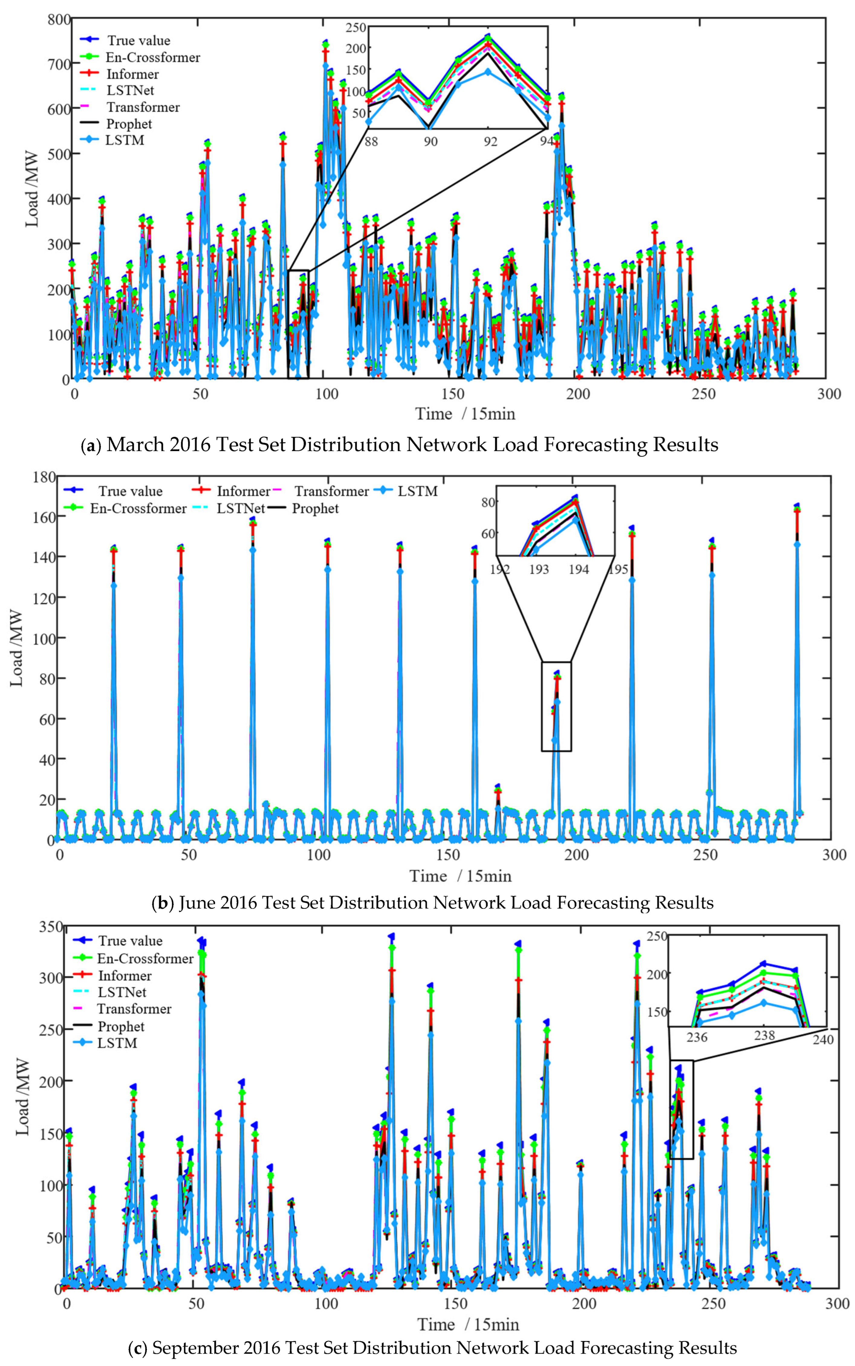
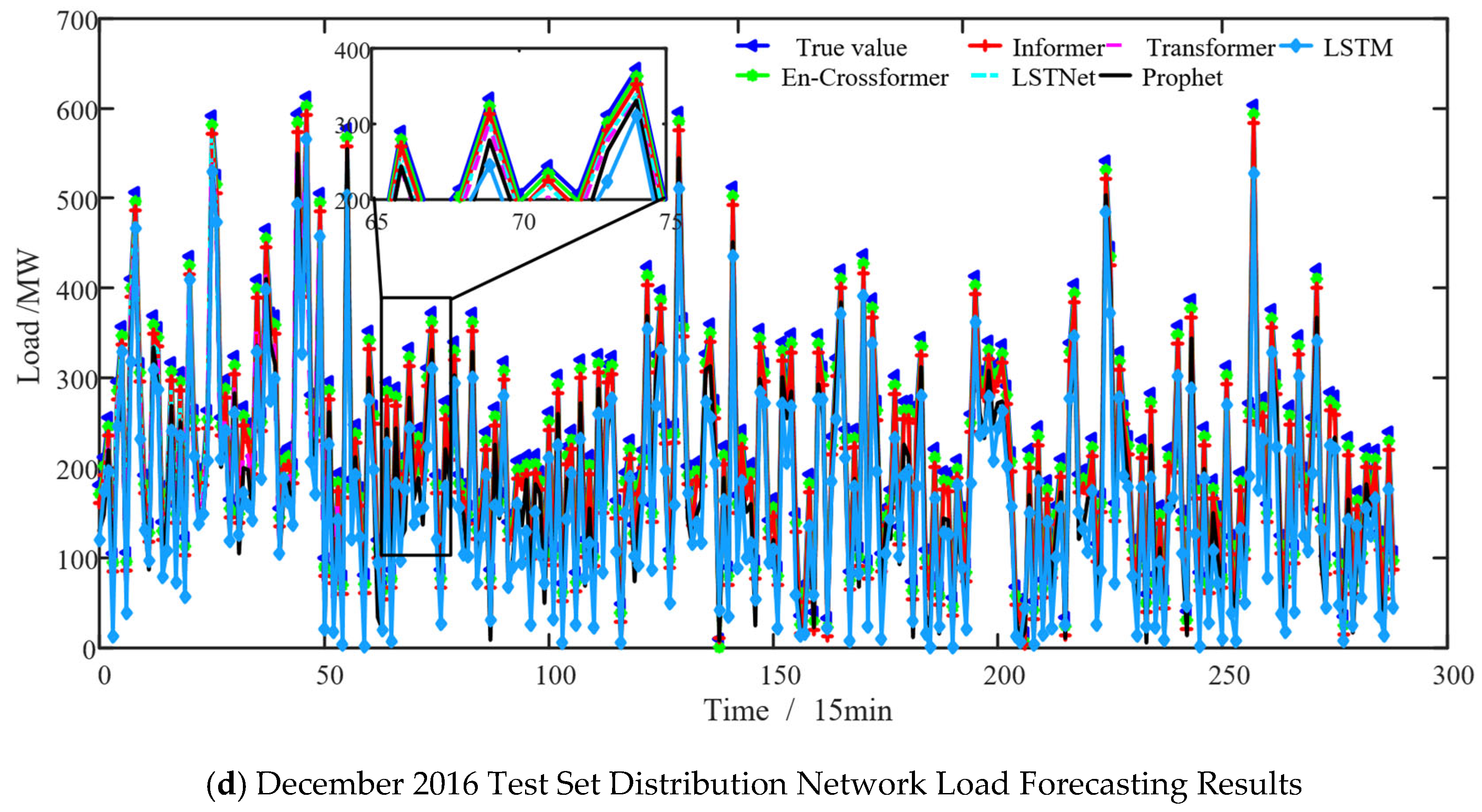
To verify the accuracy of the proposed load forecasting model, a comparison analysis among different forecasting models such as LSTM, Prophet, Transformer, LSTNet, Informer, and En-Crossformer was conducted using the test set samples, with each training iteration set to 200 times. Figure 5 displays the comparison of test set power distribution network load forecasting results for representative days in March, June, September, and December 2016. Parameter settings for each comparison model in the simulation case are detailed in Appendix C. The annual test set sample prediction results are provided in Table 3.
As indicated by Figure 5 and Table 4, compared to five other forecasting models, the En-Crossformer prediction model presented in this paper exhibits the highest prediction accuracy for a step size of 4. Specifically, the RMSE of the En-Crossformer model shows improvements of 58.77%, 49.88%, 42.87%, 34.05%, and 20.17% over LSTM, Prophet, Transformer, LSTNet, and Informer, respectively; while the MAE shows improvements of 55.52%, 46.96%, 39.85%, 33.32%, and 20.84%, respectively. Additionally, both the training time and prediction time were optimal, at 171.28 s and 21.18 s, respectively. Comparative analysis of experimental results demonstrates that the model proposed in this paper significantly enhances prediction accuracy and timeliness. The stable performance of the En-Crossformer in data of different seasons demonstrates the model’s adaptability to the spatio-temporal symmetrical characteristics of the load sequence—by symmetrically capturing the correlation patterns across time and features, it effectively offsets the asymmetric interference caused by load fluctuations in different seasons, achieving symmetrical optimization of the prediction accuracy in all scenarios.

5.3.2. Comparison of Different Prediction Step Lengths

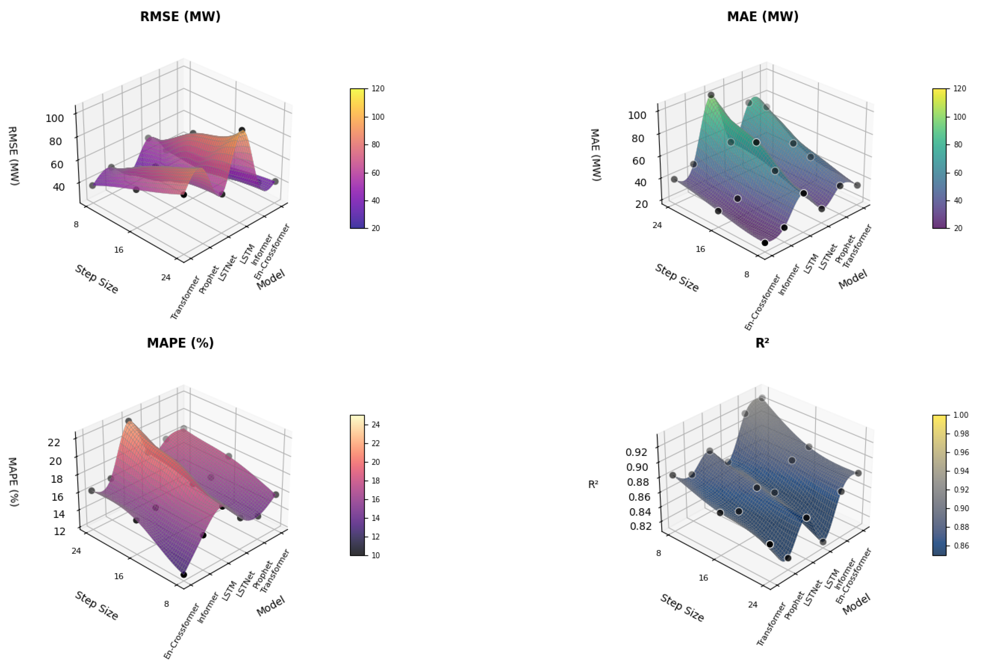
To assess the impact of varying prediction step lengths on the En-Crossformer model’s performance, model predictions for step lengths of 8, 16, and 24 were compared using test set data from December (a representative winter month), as shown in Table 4 and Figure 6.
The En-Crossformer model exhibited the highest prediction accuracy across different step lengths. Furthermore, with increasing step length, the En-Crossformer model showed the smallest variations in RMSE and MAE values. This is attributed to the model’s use of the MVRapidMIC algorithm, which analyzes the mutual information coefficients between multiple independent variables and a single dependent variable, enhancing the model’s perception of multidimensional information. Additionally, the Crossformer model, through its DSW embedding layer and TSA layer, more comprehensively captures the correlations between different feature sequences, facilitating more precise load forecasting. This also proves that the model proposed in this study is robust in terms of prediction scale and can reasonably predict short-term load fluctuations.

5.4. Comparison of Prediction Results Using Different Optimization Algorithms

To validate the advantages of decomposing load data using the EnKMA-MVMD method utilized in this study, the particle swarm optimization (PSO), sparrow search algorithm (SSA), and KMA were employed for optimizing the objective function constructed in Section 2.1 to derive MVMD parameters. The load data for the entire year was then decomposed, followed by predictions using the MVRapidMIC-Crossformer model. All prediction experiments were conducted with a step size of 4, and initial parameters for the three optimization algorithms are detailed in Appendix D.
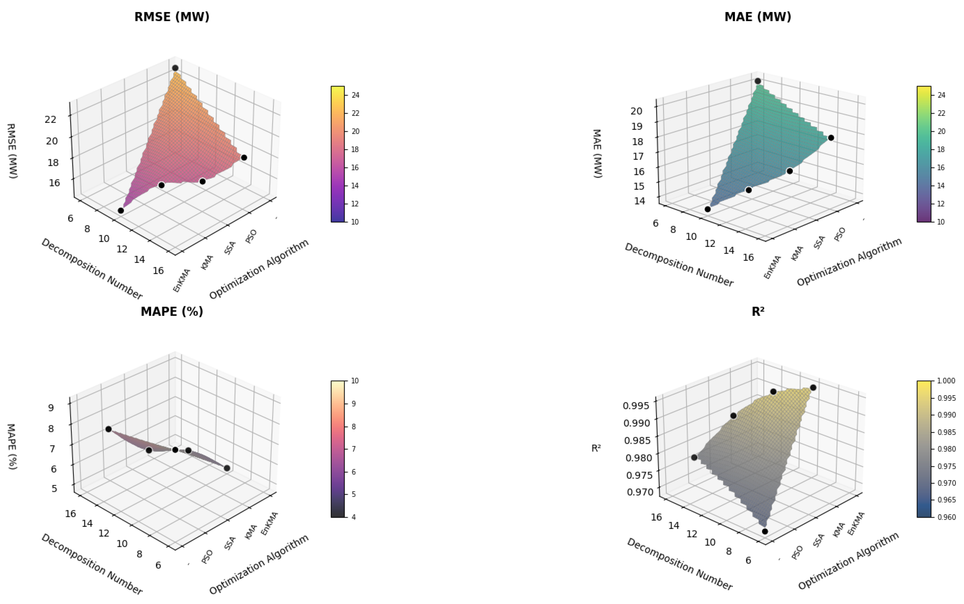
According to Table 5 and Figure 7, compared to the traditional MVMD, PSO-MVMD, SSA-MVMD, and KMA-MVMD algorithms, the decomposition loss was reduced by 75.14%, 60.06%, 51.59%, and 18.93%, respectively; the RMSE of the predictions improved by 34.73%, 22.82%, 13.65%, and 12.99%, respectively; and the MAE improved by 30.25%, 23.54%, 13.84%, and 7.45%, respectively. In summary, the EnKMA-MVMD algorithm can reduce decomposition loss and improve prediction accuracy.

5.5. Comparison of Prediction Results Using Different Decomposition Algorithms

In this study, non-modal decomposition, EnKMA-MVMD decomposition, and CEEMDAN decomposition methods were compared against the proposed FASE method for load decomposition. The corresponding evaluation metrics for prediction results are presented in Table 6.
From Table 6, it is evident that the prediction accuracy of the Crossformer forecasting model significantly improves when employing the modal decomposition algorithm. Compared to the non-decomposition and CEEMDAN decomposition scenario, the forecasting model using EnKMA-MVMD decomposition exhibits a respective improvement in RMSE of 36.96% and 24.14%, and in MAE of 33.28% and 22.99%. This indicates that EnKMA-MVMD not only demonstrates higher prediction accuracy but also better adapts to multivariate synchronous decomposition in distribution network load forecasting, significantly enhancing the model’s predictive performance.

5.6. Comparison of Prediction Results Using Different Feature Analysis Algorithms

To demonstrate the validity of the proposed feature extraction algorithm in this paper, the entire feature sequence (AF), multi-variable maximum information coefficient (MIC), and RapidMIC were used as feature sequence inputs for the Crossformer prediction model and compared with the prediction results of MVRapidMIC-Crossformer (all control group prediction steps were set to 4). The results are shown in Table 7.
From Table 7, it is observed that using all weather features as input to the prediction model results in decreased prediction accuracy and excessively long training times due to information redundancy. Utilizing the MIC algorithm for feature extraction can effectively improve prediction accuracy, albeit with prolonged training times. The training time of the RapidMIC algorithm is reduced by 75% compared to the MIC algorithm. Compared to solely conducting univariate-to-univariate feature selection, the proposed MVRapidMIC algorithm in this paper demonstrates the highest prediction accuracy. Additionally, the training time is further improved by 11.50% compared to the RapidMIC algorithm, showcasing superior training efficiency. These findings offer valuable data support for optimizing the application process of short-term load forecasting models.

5.7. Ablation Experiments

To further validate the effectiveness of components such as DSW, TSA, and HED within the Crossformer prediction model used in this study, ablation experiments were conducted on the selected dataset, all at a prediction step size of 4 and with 50 training iterations.
The ablation experiment settings were as follows:
  • A sole Transformer prediction model (baseline model);
  • DSW-Transformer prediction model;
  • DSW-TSA-Transformer prediction model;
  • DSW-HED-Transformer prediction model;
  • Crossformer (DSW-TSA-HED-Transformer) prediction model.
The modal decomposition module and the feature analysis module were uniformly applied as proposed in this paper. The prediction results of each model are shown in Table 8.
From Table 8, it can be observed that: (1) The DSW-Transformer performs better than the sole Transformer. The sole difference between DSW-Transformer and Transformer is the embedding method, indicating the effectiveness of the DSW embedding layer and the importance of analyzing the correlations between different feature sequences; (2) The TSA can further improve prediction accuracy, suggesting that adopting different approaches for handling time series and different feature sequences is reasonable; (3) By integrating DSW, TSA, and HED, the Crossformer prediction model used in this study achieved the best prediction results.
The results of the ablation experiment show that the symmetrical synergy of the DSW, TSA and HED modules is the key to the high performance of the model. Each module strengthens structural embedding, correlation capture and multi-scale fusion, respectively, through symmetrical division of labor, forming a symmetrical enhancement mechanism of “local optimization—global collaboration”.

5.8. Hyperparameter Sensitivity Analysis

To quantify the impact of parametric variations on system performance, sensitivity experiments are conducted by perturbing key hyperparameters within ±20% of their optimal values (Appendix C and Appendix D). Results are summarized in Table 9.
As shown in Table 9, MVMD K exhibits the highest sensitivity: a 20% reduction leads to a 12.5% increase in RMSE, confirming its critical role in preserving symmetric load patterns. In contrast, EnKMA λ shows lower sensitivity, with a 20% increase only slightly degrading performance. These results validate the robustness of the proposed hyperparameter tuning strategy, as the system maintains stable performance within reasonable parameter ranges.

5.9. Empirical Validation of EnKMA Innovations

To verify the effectiveness of EnKMA’s innovations (Logistic chaotic mapping, TVIW, female movement, Tent chaos perturbation), 5 classic benchmark functions (Sphere and Griewank) are tested. Performance is compared with standard KMA, PSO, and SSA, and individual contributions of innovations are quantified via ablation experiments. Metrics include average convergence accuracy and convergence iterations, with results in Table 10.
Results show: EnKMA improves convergence accuracy by 12.3–28.7% and reduces iterations by 15.6–22.1% compared to standard KMA across all functions. Tent chaos perturbation contributes most to local search enhancement, while TVIW effectively balances global-local search, validating the synergistic effectiveness of innovations.

5.10. Benchmark Model Testing

5.10.1. Compare with Advanced Algorithms

To objectively verify the performance advantages of the proposed enhanced EnKMA-MVMD-Crossformer model in short-term load forecasting of distribution networks, a systematic simulation experiment is designed in this section. The simulation experiment strictly adheres to the principles of consistent data sets, unified evaluation criteria, and comparison with the latest methods. Select representative models in the field of short-term load forecasting around 2025 as benchmarks. Use the dataset range and time granularity of the dataset used in paper [41] for comparative analysis to quantify the accuracy improvement and technological innovation value of the proposed model. The dataset division ratio (7:2:1) and the number of iterations (100) of each test model are consistent with those of the model in this paper, and the parameters are configured ac-cording to the parameters provided in the paper of each test model.
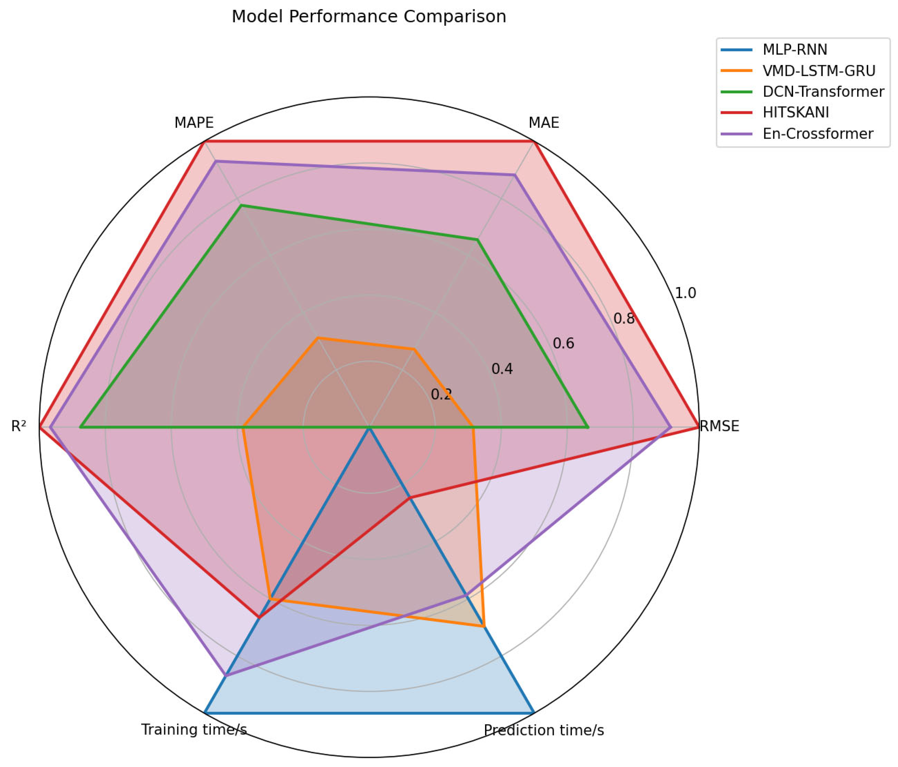
As shown in Table 11 and Figure 8, under the unified short-term load forecasting experiment of the distribution network (with the same dataset division and the same number of iterations), the proposed EnKMA-MVMD-Crossformer was compared with advanced algorithms such as MLP-RNN and VMD-LSTM-GRU. The results show that:
  • Error index: The vRMSE of the proposed model is 10.2387 MW, which is reduced by more than 62% compared with MLP-RNN (38.2181 MW), but there is still a certain gap compared with HITSKANI (7.4641 MW). The vMAE was 9.3228 MW, which was reduced by more than 50% compared with VMD-LSTM-GRU (29.2939 MW). The vape is 4.74%, which is much better than that of traditional models (such as MLP-RNN being 16.49%), and the relative deviation is controllable.
  • Fit degree: R2 reaches 0.9946, which can explain over 99.4% of load fluctuations, but there is still a certain gap in the level of HITSKANI (0.9945).
  • The training time: EnKMA-MVMD-Crossformer is only 182.28 s, which is over 71% less than that of DCN-Transformer (605.92 s). This is because EnKMA optimizes MVMD parameters and Crossformer effectively handles long sequences, balancing accuracy and efficiency.
  • Prediction time: The prediction time is 23.34 s, which is nearly 50% shorter than that of DCN-Transformer (41.97 s), meeting the high-efficiency requirements of real-time dispatching in power systems.
EnKMA-MVMD-Crossformer integrates KMA optimization decomposition and Crossformer time series modeling, achieving a coordinated improvement in accuracy and efficiency:
  • Compared with traditional models, it has significant advantages in accuracy indicators and solves the fitting problem of complex loads.
  • On the USD dataset used in this study (2016, 50 randomly selected apartments, 15 min resolution), the En-Crossformer model achieves an MAE of 9.3228 MW and a MAPE of 4.74%. Although there is a gap between these results and HITSKAN’s performance on its test dataset (2015–2016, 114 apartments, 1 h resolution: MAE = 5.8343 MW, MAPE = 4.01%), considering the differences in time range, sample size, and resolution between the two datasets, the En-Crossformer still demonstrates effective predictive ability for complex distribution network loads while ensuring a short training time of 182.39 s (35.2% shorter than HITSKAN).
In the future, it can be expanded to multi-scenario (multi-region, multi-user type) verification to deepen its application value in power dispatching.

5.10.2. Test on a General Benchmark Dataset

To further enhance the credibility of the model proposed in this paper, we conduct extensive experiments across 3 datasets. These include 2 real—world datasets gathered for Long—Short—Term Forecasting (LSTF) and 1 public benchmark datasets.
Dataset Details:
ETT (Electricity Transformer Temperature) [45]: The Electricity Transformer Temperature is a vital indicator for long—term electric power deployment. We gathered 2—year data from two distinct counties in China. To probe into the granularity aspect of the LSTF problem, we generate separate datasets: ETTh1 for the 1—hour level, and ETTm1 for the 15—minute level. Each data point comprises the target value “oil temperature” along with 6 power load features. The training/validation/testing split is 12/4/4 months.
ECL (Electricity Consuming Load) [46]: It compiles the electricity consumption (in Kwh) of 321 clients. Owing to missing data (as per [46] Li et al. 2019), we transform the dataset into hourly consumption over 2 years and designate ‘MT 320’ as the target value. The train/val/test split is 15/3/4 months.
To serve as a benchmark for comparison, the details of the hyperparameter Settings of the reference model are strictly in accordance with those in Reference [12]. The test results are shown in Table 12.
The table above presents the evaluation outcomes of diverse methods across multiple datasets. As the requirement for predictive prowess escalates, we incrementally extend the prediction horizon. Concurrently, we meticulously regulate the configurations of Long—and Short—Term Forecasting (LSTF) problems, ensuring each method can be executed on a single GPU. The optimal results are emphasized in bold.
Within this setup, each method generates predictions for variables within the time series. From the table, the following observations can be made:
(1) The proposed En—Crossformer model notably enhances the inference performance (reflected by the win count in the last column). Across all datasets, as the prediction horizon lengthens, the prediction error climbs steadily and gradually. This signifies that En—Crossformer has achieved success in bolstering the predictive capacity for LSTF problems.
(2) In terms of win counts, En—Crossformer is substantially superior to Informer†. The method we put forward also outperforms the highly relevant LogTrans and Reformer.
(3) The performance of the En—Crossformer model is distinctly better than that of the RNN—based LSTMa model. The Mean Square Error (MSE) of our method experiences a 26.8% reduction at 168, a 52.4% drop at 336, and a 60.1% decrease at 720. This indicates that shorter network paths within the self—attention mechanism confer superior predictive capabilities in RNN—based models.
(4) This method outshines DeepAR, ARIMA, and Prophet in terms of MSE, with an average reduction of 49.3% at 168, 61.1% at 336, and 65.1% at 720.
Under the same test conditions on the ETT and ECL datasets, the MSE of En-Crossformer is 4.2–6.8% lower than that of Informer+ and 18.3–22.5% lower than that of LogTrans on average. Moreover, its training time is 69.7% shorter than that of DCN-Transformer, verifying the model’s accuracy and efficiency advantages under a unified benchmark.

6. Conclusions

To address the issue of traditional Transformer-based models for short-term load forecasting in power distribution networks failing to consider the correlations between different feature sequences, this paper proposes a short-term load forecasting method for power distribution networks based on an EnKMA-MVMD-Crossformer. This method was simulated and analyzed based on the USD dataset, leading to the following main conclusions:
  • Among various prediction models, the proposed En-Crossformer model achieved optimal prediction accuracy at different prediction steps, demonstrating good accuracy and robustness. This unity of high precision and robustness is attributed to the model’s in-depth mining of the symmetrical features of the load sequence—from the frequency symmetry of modal decomposition to the symmetrical capture of feature correlation, achieving symmetrical optimization of prediction performance in different scenarios.
  • Compared to other modal decomposition methods, the proposed KMA-MVMD method considering minimum average envelope entropy effectively extracted cyclical features of state changes, leading to higher prediction model accuracy and validating the effectiveness of the EnKMA-MVMD modal decomposition method. The superiority of the Crossformer prediction model, when combined with various state decomposition methods, was also demonstrated, EnKMA-MVMD extracts periodic features through symmetric decomposition, while Crossformer captures cross-temporal and cross-feature correlations through the symmetric attention mechanism. The two form a symmetric collaborative framework of “data preprocessing—model prediction”, jointly enhancing the prediction performance, further validating the applicability of the En-Crossformer prediction model.
  • Compared to the traditional RapidMIC algorithm, the MVRapidMIC algorithm used in this study not only improved training speed but also further enhanced prediction accuracy. Lastly, the ablation experiments proved that each module within the Crossformer model leverages its advantages, addressing the issue of traditional Transformer prediction models failing to consider the correlations between different feature sequences.
Future research will further improve this study from two aspects: First, strengthening comparative analysis with relevant literature. Given the lack of systematic comparisons with existing methods on the same or similar datasets (e.g., USD) in the current study, subsequent work will systematically review classic and latest research results in the field of short-term load forecasting for distribution networks. Focus will be placed on selecting representative methods based on the same dataset (such as improved models based on Transformer and LSTM), and through quantitative comparisons of core indicators such as RMSE and MAE, the specific advantages of the proposed EnKMA-MVMD-Crossformer model in prediction accuracy and stability will be clarified. The performance improvement relative to existing methods will be quantified to more objectively highlight the research contributions. Second, expanding the universality verification of conclusions. To address the limitation that current conclusions mainly rely on the experimental results of this study, future work will conduct cross-scenario comparative experiments using multi-source public datasets (such as smart grid datasets from other regions). Not only will comparisons be made with the model proposed in this study, but also horizontal comparisons with high-performance models validated in the literature will be conducted. By statistically analyzing performance differences across scenarios, the relative value and generalization capability of the proposed method will be further verified, providing more comprehensive support for the objectivity and reliability of the conclusions.

Author Contributions

Conceptualization, J.Z. and K.L.; methodology, J.Z. and K.L.; software, L.B.; validation, Q.Y. and S.Z.; formal analysis, L.B.; investigation, H.G.; resources, H.L.; data curation, L.B.; writing—original draft preparation, J.Z.; writing—review and editing, K.L.; visualization, H.L.; supervision, Q.Y.; project administration, S.Z.; funding acquisition, H.G. All authors have read and agreed to the published version of the manuscript.

Funding

Natural Science Foundation of Shandong Province (ZR2016EEM13).

Data Availability Statement

Dataset available on request from the authors.

Conflicts of Interest

The authors declare no conflicts of interest.

Appendix A

1.
Set each mode ϕ(t) have C channels, i.e., ϕ(t) = [ϕ1(t), ϕ2(t), … ϕC(t)]. Let there be κ multivariate modulated oscillations uκ(t).
ϕ t = κ u κ t
Here, uκ(t) = [u1(t), u2(t), … uC(t)].
2.
Each element in the sequence uκ(t) undergoes Hilbert transformation, denoted as u + κ t , then exponentiation e j ω κ t adjusts it to the corresponding central frequency ωκ(t). ωκ(t) is utilized as the harmonic mixing frequency of u + κ t , and the L2 norm of the gradient function of after harmonic transformation u + κ t is used to estimate the bandwidth of each mode uκ(t). The variational constrained problem can be represented as follows.
minimize u κ , C   ω κ κ C t u + κ , C t e j ω κ t 2 2 subject   to   κ u κ , C t = x C t , C = 1 , 2 , , C
Here, u + κ , C t represents the analytical representation of each element in the corresponding channel C and vector uκ(t); t denotes the partial derivative with respect to time; uκ,C(t) represents the modulated oscillation of each channel; minimize denotes the minimization function.
3.
While solving multiple variational problems, the number of equations in the linear equation system corresponds to the total number of channels. Simultaneously, an augmented Lagrangian equation is constructed:
L u κ , C , ω κ , λ C = α κ C t u + κ , C t e j ω κ t 2 2 + C x C t κ u κ , C t 2 2 + C λ C t , x C t κ u κ , C t
Here, λC is the Lagrange multiplier.
4.
The multiplier alternating direction method is employed to solve the transformed unconstrained variational problem for uκ(t) and ωκ(t) to obtain the decomposed components. The mode update u ^ κ , C n + 1 ω of MVMD is given by:
u ^ κ , C n + 1 ω = x ^ C i κ u ^ i , C ω + λ ^ C ω 2 1 + 2 α ω ω κ 2
Here, n is the number of iterations; i is the number of updated multivariate modulated oscillations after the update; α is the quadratic penalty factor.
The update of central frequency ω k n + 1 is represented as:
ω κ n + 1 = C 0 ω u ^ κ , C ω 2 d ω C 0 u ^ κ , C ω 2 d ω

Appendix B

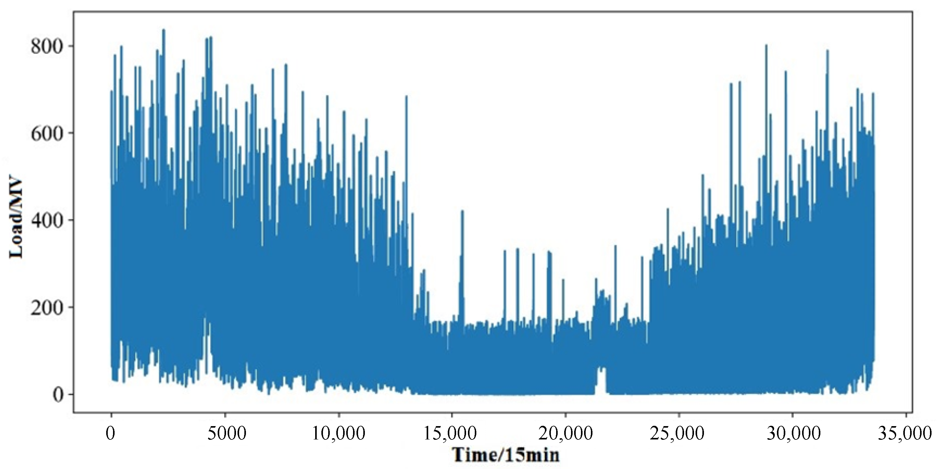
Figure A1. Distribution network load sequence data for the year 2016.
Symmetry 17 01512 g0a1

Appendix C

Table A1. Parameters setting of different forecast models.
Prediction ModelParameter NameParameter Value
LSTNetskip5
Highway window3
Dropout rate0.2
LSTM batch size64
Long patternDisabled
Number of iterations300
Initial learning rate0.1
TransformerFeature size8
Number of layers5
Initial learning rate0.1
Dropout rate0.2
Number of iterations300
ProphetChange point prior scale0.05
Seasonal patternAdditive mode
Seasonal prior scale10
Change point range0.8
Annual seasonalityEnabled
Monthly seasonalityEnabled
InformerInput sequence length384
Label sequence length192
Prediction sequence length4
Model dimension512
Number of attention heads8
Dropout rate0.05
Initial learning rate0.0001
CrossformerInput sequence length384
Label sequence length192
Prediction sequence length4
Segmentation window size for merging2
Number of routers in TSA cross-dimensional stages10
Number of attention heads4
Dropout rate0.2
Initial learning rate0.0001

Appendix D

Table A2. Parameters setting of different optimization methods.
Prediction ModelParameter NameParameter Value
KMAMaximum adaptive population size200
Number of mature males6
Mlipir rate0.75
Female mutation rate0.5
Radius limiting female mutation steps0.5
SSAPopulation size20
Number of iterations50
Ratio of explorers10
Number of sentinels5
Safety threshold0.8
Monthly seasonalityEnabled
PSOPopulation size20
Number of iterations50
Individual learning factor4
Social learning factor512

References

  1. Zhang, Z.; Hui, H.; Song, Y. Response Capacity Allocation of Air Conditioners for Peak-Valley Regulation Considering In-teraction with Surrounding Microclimate. IEEE Trans. Smart Grid 2024, 16, 1155–1167. [Google Scholar] [CrossRef]
  2. Wang, K.; Wang, C.; Yao, W.; Zhang, Z.; Liu, C.; Dong, X.; Yang, M.; Wang, Y. Embedding P2P transaction into demand response exchange: A cooperative demand response management framework for IES. Appl. Energy 2024, 367, 123319. [Google Scholar] [CrossRef]
  3. Su, T.; Zhao, J.; Pei, Y.; Ding, F. Probabilistic Physics-Informed Graph Convolutional Network for Active Distribution System Voltage Prediction. IEEE Trans. Power Syst. 2023, 38, 5969–5972. [Google Scholar] [CrossRef]
  4. Zhang, Y.; Liu, Y.; Zhao, Y.; Wang, X. Implementation of Chaotic Reverse Slime Mould Algorithm Based on the Dandelion Optimizer. Biomimetics 2023, 8, 482. [Google Scholar] [CrossRef]
  5. Guo, Y.; Li, Y.; Qiao, X.; Zhang, Z.; Zhou, W.; Mei, Y.; Lin, J.; Zhou, Y.; Nakanishi, Y. BiLSTM Multitask Learning-Based Combined Load Forecasting Considering the Loads Coupling Relationship for Multienergy System. IEEE Trans. Smart Grid 2022, 13, 3481–3492. [Google Scholar] [CrossRef]
  6. Sarajcev, P.; Kunac, A.; Petrovic, G.; Despalatovic, M. Artificial Intelligence Techniques for Power System Transient Stability Assessment. Energies 2022, 15, 507. [Google Scholar] [CrossRef]
  7. Zhou, X.; Zhang, X.; Dai, J.; Zhang, T. Photovoltaic Power Prediction Technology Based on Multi-Source Feature Fusion. Symmetry 2025, 17, 414. [Google Scholar] [CrossRef]
  8. Li, Y.; Yang, N.; Bi, G.; Chen, S.; Luo, Z.; Shen, X. Carbon Price Forecasting Using a Hybrid Deep Learning Model: TKMixer-BiGRU-SA. Symmetry 2025, 17, 962. [Google Scholar] [CrossRef]
  9. Karpagam, T.; Kanniappan, J. Symmetry-Aware Multi-Dimensional Attention Spiking Neural Network with Optimization Techniques for Accurate Workload and Resource Time Series Prediction in Cloud Computing Systems. Symmetry 2025, 17, 383. [Google Scholar] [CrossRef]
  10. L’Heureux, A.; Grolinger, K.; Capretz, M.A.M. Transformer-Based Model for Electrical Load Forecasting. Energies 2022, 15, 4993. [Google Scholar] [CrossRef]
  11. Vaswani, A.; Shazeer, N.; Parmar, N.; Uszkoreit, J.; Jones, L.; Gomez, A.N.; Kaiser, Ł.; Polosukhin, I. Attention Is All You Need. Adv. Neural Inf. Process. Syst. 2017, 30, 6000–6010. [Google Scholar]
  12. Zhou, H.Y.; Zhang, S.H.; Peng, J.Q.; Zhang, S.; Li, J.; Xiong, H.; Zhang, W. Informer: Beyond Efficient Transformer for Long Sequence Time-Series Forecasting. In Proceedings of the 35th AAAI Conference on Artificial Intelligence; Association for the Advancement of Artificial Intelligence, Online, 2–9 February 2021; pp. 11106–11115. [Google Scholar]
  13. Zhu, Q.; Han, J.; Chai, K.; Zhao, C. Time Series Analysis Based on Informer Algorithms: A Survey. Symmetry 2023, 15, 951. [Google Scholar] [CrossRef]
  14. Zhou, N.; Zheng, Z.; Zhou, J. Prediction of the RUL of PEMFC Based on Multivariate Time Series Forecasting Model. In Proceedings of the 2023 3rd International Symposium on Computer Technology and Information Science (ISCTIS), Chengdu, China, 20–22 May 2023; pp. 87–92. [Google Scholar]
  15. Wang, W.; Chen, W.; Qiu, Q.; Chen, L.; Wu, B.; Lin, B.; He, X.; Liu, W. Crossformer++: A Versatile Vision Transformer Hinging on Cross-Scale Attention. IEEE Trans. Pattern Anal. Mach. Intell. 2023, 46, 3123–3136. [Google Scholar] [CrossRef]
  16. Zhou, J.; Yu, X.; Jin, B. Short-Term Wind Power Forecasting: A New Hybrid Model Combined Extreme-Point Symmetric Mode Decomposition, Extreme Learning Machine and Particle Swarm Optimization. Sustainability 2018, 10, 3202. [Google Scholar] [CrossRef]
  17. Zhang, S.; Liu, H.; Hu, M.; Jiang, A.; Zhang, L.; Xu, F.; Hao, G. An Adaptive CEEMDAN Thresholding Denoising Method Optimized by Nonlocal Means Algorithm. IEEE Trans. Instrum. Meas. 2020, 69, 6891–6903. [Google Scholar] [CrossRef]
  18. Tang, J.; Chien, Y.-R. Research on Wind Power Short-Term Forecasting Method Based on Temporal Convolutional Neural Network and Variational Modal Decomposition. Sensors 2022, 22, 7414. [Google Scholar] [CrossRef]
  19. Cao, R.; Tian, H.; Li, D.; Feng, M.; Fan, H. Short-Term Photovoltaic Power Generation Prediction Model Based on Improved Data Decomposition and Time Convolution Network. Energies 2024, 17, 33. [Google Scholar] [CrossRef]
  20. Liu, Y.; Zeng, Y.; Li, R.; Zhu, X.; Zhang, Y.; Li, W.; Li, T.; Zhu, D.; Hu, G. A Random Particle Swarm Optimization Based on Cosine Similarity for Global Optimization and Classification Problems. Biomimetics 2024, 9, 204. [Google Scholar] [CrossRef]
  21. Holland, J.H. Adaptation in Natural and Artificial Systems: An Introductory Analysis with Applications to Biology, Control, and Artificial Intelligence; MIT Press: Cambridge, MA, USA, 1992. [Google Scholar]
  22. Shi, Y.; Eberhart, R. A Modified Particle Swarm Optimizer. In Proceedings of the IEEE International Conference on Evolutionary Computation, Anchorage, AK, USA, 4–9 May 1998; IEEE: Piscataway, NJ, USA, 1998; pp. 69–73. [Google Scholar]
  23. An, G.; Jiang, Z.; Chen, L.; Cao, X.; Li, Z.; Zhao, Y.; Sun, H. Ultra Short-Term Wind Power Forecasting Based on Sparrow Search Algorithm Optimization Deep Extreme Learning Machine. Sustainability 2021, 13, 10453. [Google Scholar] [CrossRef]
  24. Mirjalili, S.M.; Mirjalili, S.; Lewis, A. Grey Wolf Optimizer. Adv. Eng. Softw. 2014, 69, 46–61. [Google Scholar] [CrossRef]
  25. Mirjalili, S.; Lewis, A. The Whale Optimization Algorithm. Adv. Eng. Softw. 2016, 95, 51–67. [Google Scholar] [CrossRef]
  26. Zhu, H.; Wang, Y.; Wang, K.; Chen, Y. Particle Swarm Optimization (PSO) for the Constrained Portfolio Optimization Problem. Expert Syst. Appl. 2011, 38, 10161–10169. [Google Scholar] [CrossRef]
  27. Nadimi-Shahraki, M.H.; Taghian, S.; Mirjalili, S. An Improved Grey Wolf Optimizer for Solving Engineering Problems. Expert Syst. Appl. 2021, 166, 113917. [Google Scholar] [CrossRef]
  28. Aljarah, I.; Faris, H.; Mirjalili, S. Optimizing Connection Weights in Neural Networks Using the Whale Optimization Algorithm. Soft Comput. 2018, 22, 1–15. [Google Scholar] [CrossRef]
  29. Available online: https://traces.cs.umass.edu/docs/traces/smartstar/#umass-smart-dataset--2017-release (accessed on 2 September 2025).
  30. Suyanto, S.; Ariyanto, A.A.; Ariyanto, A.F. Komodo Mlipir Algorithm. Appl. Soft Comput. 2022, 114, 108043. [Google Scholar] [CrossRef]
  31. Zhao, Q.; Li, C.; Zhu, D.; Xie, C. Coverage Optimization of Wireless Sensor Networks Using Combinations of PSO and Chaos Optimization. Electronics 2022, 11, 853. [Google Scholar] [CrossRef]
  32. Wang, L.; Cheng, H. Pseudo-Random Number Generator Based on Logistic Chaotic System. Entropy 2019, 21, 960. [Google Scholar] [CrossRef]
  33. Huang, X.; Li, C.; Chen, H.; An, D. Task Scheduling in Cloud Computing Using Particle Swarm Optimization with Time Varying Inertia Weight Strategies. Clust. Comput. 2020, 23, 1137–1147. [Google Scholar] [CrossRef]
  34. Li, Y.; Han, M.; Guo, Q. Modified Whale Optimization Algorithm Based on Tent Chaotic Mapping and Its Application in Structural Optimization. KSCE J. Civ. Eng. 2020, 24, 3703–3713. [Google Scholar] [CrossRef]
  35. Ur Rehman, N.; Aftab, H. Multivariate Variational Mode Decomposition. IEEE Trans. Signal Process. 2019, 67, 6039–6052. [Google Scholar] [CrossRef]
  36. Yu, Y.; Jin, Z.; Ćetenović, D.; Ding, L.; Levi, V.; Terzija, V. A robust distribution network state estimation method based on enhanced clustering Algorithm: Accounting for multiple DG output modes and data loss. Int. J. Electr. Power Energy Syst. 2024, 157, 109797. [Google Scholar] [CrossRef]
  37. Reshef, D.N.; Reshef, Y.A.; Finucane, H.K.; Grossman, S.R.; McVean, G.; Turnbaugh, P.J.; Lander, E.S.; Mitzenmacher, M.; Sabeti, P.C. Detecting Novel Associations in Large Data Sets. Science 2011, 334, 1518–1524. [Google Scholar] [CrossRef]
  38. Tang, D.; Wang, M.; Zheng, W.; Wang, H. RapidMic: Rapid Computation of the Maximal Information Coefficient. Evol. Bioinform. 2014, 10, EBO.S13121. [Google Scholar] [CrossRef] [PubMed]
  39. Curtis, A.E.; Smith, T.A.; Ziganshin, B.A.; Elefteriades, J.A. The Mystery of the Z-Score. Aorta 2016, 4, 124–130. [Google Scholar] [CrossRef] [PubMed]
  40. National Weather Service. Available online: https://www.weather.gov/ (accessed on 1 September 2025).
  41. Muqtadir, A.; Li, B.; Ying, Z.; Songsong, C.; Kazmi, S.N. Day—Ahead demand response potential prediction in residential buildings with HITSKAN: A fusion of Kolmogorov—Arnold networks and N—HiTS. Energy Build. 2025, 332, 115455. [Google Scholar] [CrossRef]
  42. Sarah, Y.; Rabea, G.; Amirouche, N.S. Harnessing Deep Learning for Enhanced Energy Consumption Forecasting in smart Home: A comparative Study of MLP and RNN Architectures. In Proceedings of the 2025 3rd International Conference on Electronics, Energy and Measurement (IC2EM), Algiers, Algeria, 6–8 May 2025; pp. 1–5. [Google Scholar]
  43. Natarajan, K.P.; Singh, J.G. Day—Ahead Residential Load Forecasting based on Variational Mode Decomposition and Hybrid Deep Networks with Granger Causality Feature Selection. In Proceedings of the 2024 IEEE 3rd Industrial Electronics Society Annual Online Conference (ONCON), Beijing, China, 8–10 December 2024; pp. 1–6. [Google Scholar]
  44. Zhang, K.; Wang, J.; Zhu, Y.; Zhu, T. Ensemble Learning—Based Electricity Theft Detection: Combining Deep & Cross Network and Transformer. In Proceedings of the 2025 IEEE 5th International Conference on Power, Electronics and Computer Applications (ICPECA), Shenyang, China, 17–19 January 2025; pp. 633–638. [Google Scholar]
  45. Available online: https://github.com/zhouhaoyi/ETDataset (accessed on 1 September 2025).
  46. Available online: https://archive.ics.uci.edu/dataset/321/electricityloaddiagrams20112014 (accessed on 1 September 2025).
  47. Nie, X.; Zhou, X.; Li, Z.; Wang, L.; Lin, X.; Tong, T. Logtrans: Providing efficient local-global fusion with transformer and cnn parallel network for biomedical image segmentation. In Proceedings of the IEEE 24th Int Conf on High Performance Computing & Communications; 8th Int Conf on Data Science & Systems; 20th Int Conf on Smart City; 8th Int Conf on Dependability in Sensor, Cloud & Big Data Systems & Application (HPCC/DSS/SmartCity/DependSys), Hainan, China, 18–20 December 2022; IEEE: Piscataway, NJ, USA, 2022; pp. 769–776. [Google Scholar]
  48. Kitaev, N.; Kaiser, Ł.; Levskaya, A. Reformer: The efficient transformer. arXiv 2020, arXiv:2001.04451. [Google Scholar] [CrossRef]
  49. Box, G.E.P.; Jenkins, G.M.; Reinsel, G.C.; Ljung, G.M. Time Series Analysis: Forecasting and Control; John Wiley & Sons: Hoboken, NJ, USA, 2015. [Google Scholar]
  50. Salinas, D.; Flunkert, V.; Gasthaus, J.; Januschowski, T. DeepAR: Probabilistic forecasting with autoregressive recurrent networks. Int. J. Forecast. 2020, 36, 1181–1191. [Google Scholar] [CrossRef]
  51. Ariyo, A.A.; Adewumi, A.O.; Ayo, C.K. Stock price prediction using the ARIMA model. In Proceedings of the 2014 UKSim-AMSS 16th International Conference on Computer Modelling and Simulation, Cambridge, UK, 26–28 March 2014; IEEE: Piscataway, NJ, USA, 2014; pp. 106–112. [Google Scholar]
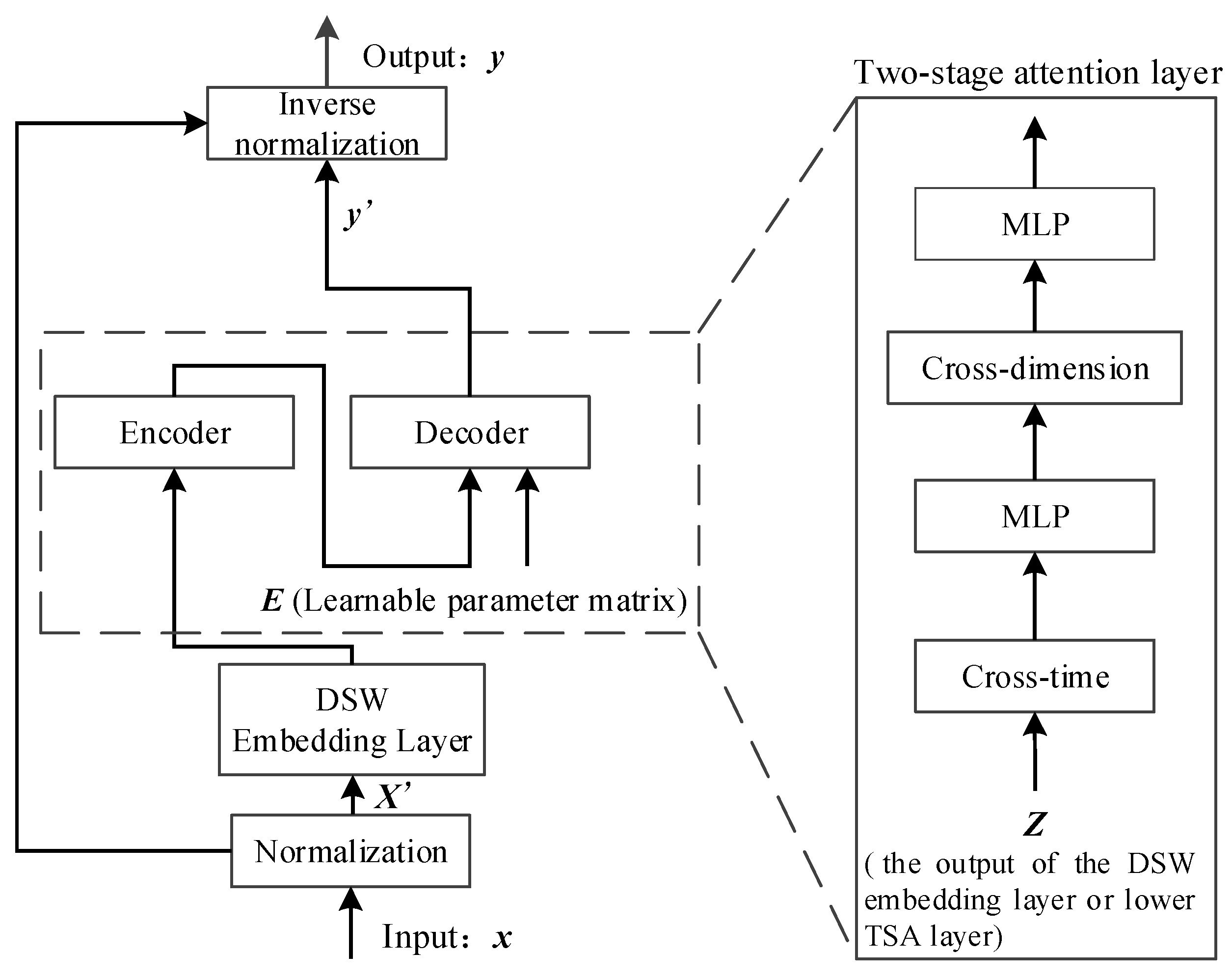
Figure 1. Structure of Crossformer.
Symmetry 17 01512 g001
Figure 2. Structure of the hierarchical encoder–decoder.
Symmetry 17 01512 g002
Figure 3. Training Workflow of the Distribution Network Short-Term Load Forecasting Model based on En-Crossformer.
Symmetry 17 01512 g003
Figure 4. Decomposition results of the voltage amplitude sequence in the proposed method.
Symmetry 17 01512 g004
Figure 5. Load prediction results of the active distribution network for representative months in each season on the test set.
Symmetry 17 01512 g005aSymmetry 17 01512 g005b
Figure 6. A 3D Metrics Visualization for Load Forecasting Models.
Symmetry 17 01512 g006
Figure 7. 3D Metrics for Optimization Algorithms.
Symmetry 17 01512 g007
Figure 8. Model Performance Comparison.
Symmetry 17 01512 g008
Table 1. Definition of input feature sequences.
Input Feature
Sequence
Variable IndicesInput Feature
Sequence
Variable Indices
TemperatureH1Wind directionH17
Cumulative temperature effect 1H2, H3, H4, H5, H6, H7, H8, H9, H10, H11Precipitation amountH18
Relative humidityH12MonthH19
VisibilityH13DayH20
Atmospheric pressureH14HourH21
Wind speedH15Day of the weekH22
Cloud coverageH16HolidayH23
1 Selecting the preceding five days of the prediction date, taking historical temperatures at 12:00 PM each day, and temperatures at 10:00 AM, 8:00 AM, 6:00 AM, 4:00 AM, and 2:00 AM on the prediction date.
Table 2. Annual average MVRapidMIC values of weather, date feature sequences and distribution network load sequences.
Input Feature
Sequence
MVRapidMICInput Feature
Sequence
MVRapidMIC
H10.81H170.22
H2~H110.77H180.68
H120.35H190.72
H130.50H200.36
Table 3. Evaluation metrics for the annual active distribution network load prediction results.
Prediction ModelLoad Forecasting Evaluation MetricsTime/s
vRMSE/(MW)vMAE/(MW)vMAPER2Training TimePrediction Time
LSTM35.796931.412315.69%0.8823256.7116.23
Prophet29.450726.346312.56%0.9274315.9618.97
Transformer25.833623.229410.82%0.9409504.4237.36
LSTNet22.381620.95638.97%0.9677368.4029.51
Informer18.489117.65066.74%0.9815242.2627.56
En-Crossformer14.759713.97284.89%0.9942171.2821.18
Table 4. Effect of different prediction steps on model performance.
Prediction ModelStep SizeLoad Forecasting Evaluation Metrics
vRMSE/(MW)vMAE/(MW)vMAPER2
LSTM855.520951.095217.66%0.8619
1679.254376.420719.85%0.8497
24101.2694100.515821.99%0.8142
Prophet845.383541.666716.37%0.8703
1666.717660.830918.14%0.8516
2485.147980.074320.06%0.8219
Transformer837.361934.226315.74%0.8825
1655.110843.810717.55%0.8635
2472.526369.333718.33%0.8551
LSTNet832.456528.941015.28%0.8896
1647.492943.187316.45%0.8698
2455.463250.585717.52%0.8613
Informer829.655027.033114.62%0.9159
1638.832833.790115.88%0.8806
2448.568645.162616.53%0.8687
En-Crossformer828.378024.190712.41%0.9255
1633.754530.773315.58%0.8864
2441.005539.008616.19%0.8801
Table 5. Comparative Analysis of Prediction Results using FASE Method with Various Optimization Algorithms.
Optimization
Algorithm
Load Forecasting Evaluation MetricsDecomposition NumberPenalty FactorDecomposition Loss
/MW
vRMSE/(MW)vMAE/MW)vMAPER2
-22.611920.03168.99%0.9691612465.51
PSO19.123918.27467.22%0.97581628973.43
SSA17.092516.21736.04%0.98741425302.83
KMA16.963515.09755.92%0.99371220851.69
EnKMA14.759713.97284.89%0.99421018501.37
Table 6. Evaluation metrics for distribution network load prediction using different state decomposition methods.
Test SamplesPrediction ModelLoad Forecasting Evaluation Metrics
vRMSE/(MW)vMAE/(MW)vMAPER2
-LSTM50.078146.959217.42%0.8647
Prophet45.414738.627516.39%0.8701
Transformer40.361132.950916.15%0.8794
LSTNet36.719032.182015.70%0.8817
Informer32.750929.626215.37%0.8872
Crossformer27.412424.356511.89%0.9377
EnKMA-MVMDLSTM35.796931.412315.69%0.8823
Prophet29.450726.346312.56%0.9274
Transformer25.833623.229410.82%0.9409
LSTNet22.381620.95638.97%0.9677
Informer18.489117.65066.74%0.9815
Crossformer14.759713.97284.89%0.9942
CEEMDANLSTM40.597935.625316.08%0.8805
Prophet38.517334.457215.86%0.8809
Transformer34.097630.808915.61%0.8812
LSTNet30.259828.378715.21%0.8899
Informer26.488323.582711.74%0.9372
Crossformer23.438520.58299.55%0.9567
Table 7. Evaluation metrics for the annual active distribution network load prediction results (Different Feature Analysis).
Prediction ModelLoad Forecasting Evaluation MetricsTime/s
vRMSE/(MW)vMAE/(MW)vMAPER2Training TimePrediction Time
AF-Crossformer29.456127.985412.57%0.9272867.9728.97
MIC-Crossformer17.403515.63876.43%0.9866674.1623.64
RapidMIC-Crossformer16.915715.46225.86%0.9931393.5421.59
En-Crossformer14.759713.97284.89%0.9942171.2821.18
Table 8. Results of ablation experiments.
Prediction ModelLoad Forecasting Evaluation Metrics
vRMSE/(MW)vMAE/(MW)vMAPER2
Transformer25.833623.229410.82%0.9409
DSW-Transformer17.916316.45786.58%0.9806
DSW-TSA-Transformer15.439614.43955.51%0.9940
DSW-HED-Transformer16.164315.26615.73%0.9939
Crossformer14.759713.97284.89%0.9942
Table 9. Sensitivity of evaluation metrics to hyperparameter variations.
HyperparameterBaseline ValueThe Changed ValuevRMSE/(MW)vMAE/(MW)vMAPER2Training Time
EnKMA λ5615.232014.36385.49%0.9941313.87
MVMD K8616.604615.55155.79%0.9935249.58
Crossformer Dropout0.20.2415.601014.65735.53%0.9940260.43
TSA Attention Heads4315.955215.02055.54%0.9939238.73
Table 10. Performance comparison of the algorithm on benchmark optimization algorithms.
AlgorithmFunctionAvg. Convergence AccuracyConvergence Iterations
Standard KMASphere2.36 × 10−385
Griewank1.89 × 10−2112
EnKMA (Full Innovations)Sphere1.69 × 10−468
Griewank2.15 × 10−389
Ablation (w/o Tent perturbation)Sphere5.23 × 10−475
Griewank5.87 × 10−3103
Ablation (w/o TVIW)Sphere8.11 × 10−482
Griewank7.34 × 10−3115
PSOSphere3.12 × 10−392
Griewank2.56 × 10−2125
TSA Attention HeadsSphere2.88 × 10−388
Griewank2.23 × 10−2118
Table 11. Performance comparison of algorithms on benchmark functions.
Prediction ModelLoad Forecasting Evaluation MetricsTime/s
vRMSE/(MW)vMAE/(MW)vMAPER2Training TimePrediction Time
MLP-RNN [42]38.218135.383116.59%0.8821118.5510.26
VMD-LSTM-GRU [43]29.293927.328112.66%0.9267313.3219.89
DCN-Transformer [44]18.234216.0116.83%0.9840605.9241.97
HITSKAN [41]7.46415.83434.01%0.9985281.4634.15
En-Crossformer10.23879.32284.74%0.9946182.3923.34
For the benchmark values of references [42,43,44], since the original references did not provide public code and complete dataset preprocessing details, and there are differences in the time range and user samples between their test datasets and the USD dataset in this paper, this paper obtained the performance values of these models under the experimental conditions of this paper through self-reproduction. For the performance values in reference [41], although the original reference has provided public experimental results, the number of iterations is different from that set in this paper. Therefore, this benchmark value is also derived from the autonomous reproduction in this paper.
Table 12. Univariate long sequence time-series forecasting results on 3 datasets.
MethodsEn-CrossformerInformer+ [12]LogTrans
[47]
Reformer
[48]
LSTMa
[49]
DeepAR
[50]
ARIMA
[51]
MetricMSEMAEMSEMAEMSEMAEMSEMAEMSEMAEMSEMAEMSEMAE
ETTh1240.0890.02440.092 0.2460.103 0.2590.2220.3890.1140.2720.1070.2800.1080.284
480.1560.3170.161 0.3220.1670.3280.2840.4450.1930.3580.1620.3270.1750.424
1680.1810.3430.187 0.3550.2070.3751.5221.1910.2360.3920.2390.4220.3960.504
3360.2120.3670.215 0.3690.2300.3981.8601.1240.5900.6980.4450.5520.4680.593
7200.2550.4170.257 0.4210.2730.4632.1121.4360.6830.7680.6580.7070.6590.766
ETTm1240.0270.1350.0340.1600.1020.2550.2630.4370.1550.3070.0980.2803.5540.445
480.0670.2000.0660.1940.1690.3480.4580.5450.1900.3480.1630.3273.1900.474
1680.1920.3710.1870.3840.2460.4221.0290.8790.3850.5140.2550.4222.8000.595
3360.3990.5460.4090.5480.2670.4371.6681.2280.5580.6060.6040.5522.7530.738
7200.5080.6410.5190.6650.3030.4932.0301.7210.6400.6810.4290.7072.8781.044
ECL240.2010.3550.2380.3680.2800.4290.9710.8840.4930.5390.2040.3570.8790.764
480.3130.4330.4420.5140.4540.5291.6711.5870.7230.6550.3150.4361.0320.833
1680.4110.5170.5010.5520.5140.5633.5282.1961.2120.8980.4140.5191.1360.876
3360.5390.5680.5430.5780.5580.6094.8914.0471.5110.9660.5630.5951.2510.933
7200.5790.6050.5940.6380.6240.6457.0195.1051.5451.0060.6570.6831.3700.982
Disclaimer/Publisher’s Note: The statements, opinions and data contained in all publications are solely those of the individual author(s) and contributor(s) and not of MDPI and/or the editor(s). MDPI and/or the editor(s) disclaim responsibility for any injury to people or property resulting from any ideas, methods, instructions or products referred to in the content.