Article

Benders Decomposition Approach for Generalized Maximal Covering and Partial Set Covering Location Problems

1
School of Mathematical Sciences, Beijing University of Posts and Telecommunications, Beijing 100876, China
2
Academy of Mathematics and Systems Science, Chinese Academy of Sciences, Beijing 100190, China
3
School of Mathematical Sciences, University of Chinese Academy of Sciences, Beijing 100049, China
*
Author to whom correspondence should be addressed.
These authors contributed equally to this work.
Symmetry 2025, 17(9), 1417; https://doi.org/10.3390/sym17091417
Submission received: 24 July 2025 / Revised: 19 August 2025 / Accepted: 22 August 2025 / Published: 1 September 2025
(This article belongs to the Section Mathematics)

Abstract

Covering problems constitute a central theme in facility location research. This study extends the classical Maximal Covering Location Problem (MCLP) and Partial Set Covering Location Problem (PSCLP) to their generalized variants, in which each demand point must be simultaneously served by multiple facilities. This generalization captures reliability requirements inherent in applications such as emergency response and robust communication networks. We first present integer programming formulations for both generalized problems, followed by equivalent reformulations that facilitate algorithmic development. Building on these, we design exact Benders decomposition algorithms that exploit structural properties of the problems to achieve enhanced scalability and computational efficiency. Computational experiments on large-scale synthetic instances with up to 200,000 demand points demonstrate that our method attains more than a threefold speedup over CPLEX. We further validate the effectiveness of the proposed approach through experiments on a real-world dataset. In addition, we compare our method with a tabu search heuristic, and the numerical results show that within a fixed time limit, our method is generally able to identify higher-quality feasible solutions. These results collectively demonstrate both the effectiveness and the practical applicability of our approach for large-scale generalized covering problems.

1. Introduction

Covering problems represent a fundamental class of facility location problems and have been extensively studied in the literature, with applications in diverse domains such as healthcare facility planning [1], disaster relief resource deployment [2], fire detection systems [3], ambulance base placement [4], bank network configuration [5], bike-sharing networks [6], and virus mitigation strategies [7]. These problems typically involve a set of demand points and a set of potential facility locations. The objective is to select a subset of facilities to be established under certain constraints, which are usually imposed either on the value of demand points that can be covered or on the total cost of facility construction. A demand point is generally considered to be covered if it lies within the service region of at least one open facility. Most commonly, the service region is assumed to be a circle centered at the facility with a predefined radius. Alternative geometries such as ring-shaped [8], square [9,10], and elliptical regions [11] have also been explored in the literature.
The Set Covering Location Problem (SCLP) [12] is one of the most well-known models in covering problems. It aims to minimize the cost required to cover all demand points. However, in many real-world applications, budget limitations often make it impossible to guarantee full coverage. This has led to the development of two widely studied extensions:
  • The Maximal Covering Location Problem (MCLP) [13], which seeks to select facility locations such that the total value of covered demand points is maximized, subject to a facility budget constraint;
  • The Partial Set Covering Location Problem (PSCLP) [14], which minimizes the required facility construction budget while ensuring that the total value of covered demand points meets or exceeds a specified covering demand.
These two problems constitute a pair of symmetric formulations; specifically, one is the counterpart of the other with the objective and constraint interchanged. In both problems, a demand point is considered covered if it is served by at least one facility. This assumption, though reasonable in some settings, may not hold in high-stakes scenarios such as healthcare facility planning [15], where the failure of a single distribution center can result in significant service disruptions, potentially leading to patient harm and public disorder. To address this, we extend the classical notion of coverage. Specifically, a demand point is considered covered only when it is simultaneously served by a number of facilities that satisfy or exceed its predefined coverage requirement (≥1). We refer to these generalized models as the Generalized Maximal Covering Location Problem (G-MCLP) and the Generalized Partial Set Covering Location Problem (G-PSCLP):
  • G-MCLP: Maximize the total value of demand points that are each served by at least their multi-coverage requirement, subject to a facility budget constraint.
  • G-PSCLP: Minimize the total facility budget while ensuring that a specified total value of demand points is each served in accordance with their multi-coverage requirement.
These generalized models arise in a variety of applications, such as the deployment of emergency vehicles [16,17], where service reliability is critical and mere reachability of a single facility is insufficient. Each demand point must be served by multiple emergency vehicles to ensure that the probability of receiving timely service remains sufficiently high. Other relevant high-reliability scenarios include vulnerable rail networks [18], police patrol area design [19], humanitarian relief supply chains [20,21], and infectious disease control models [22].
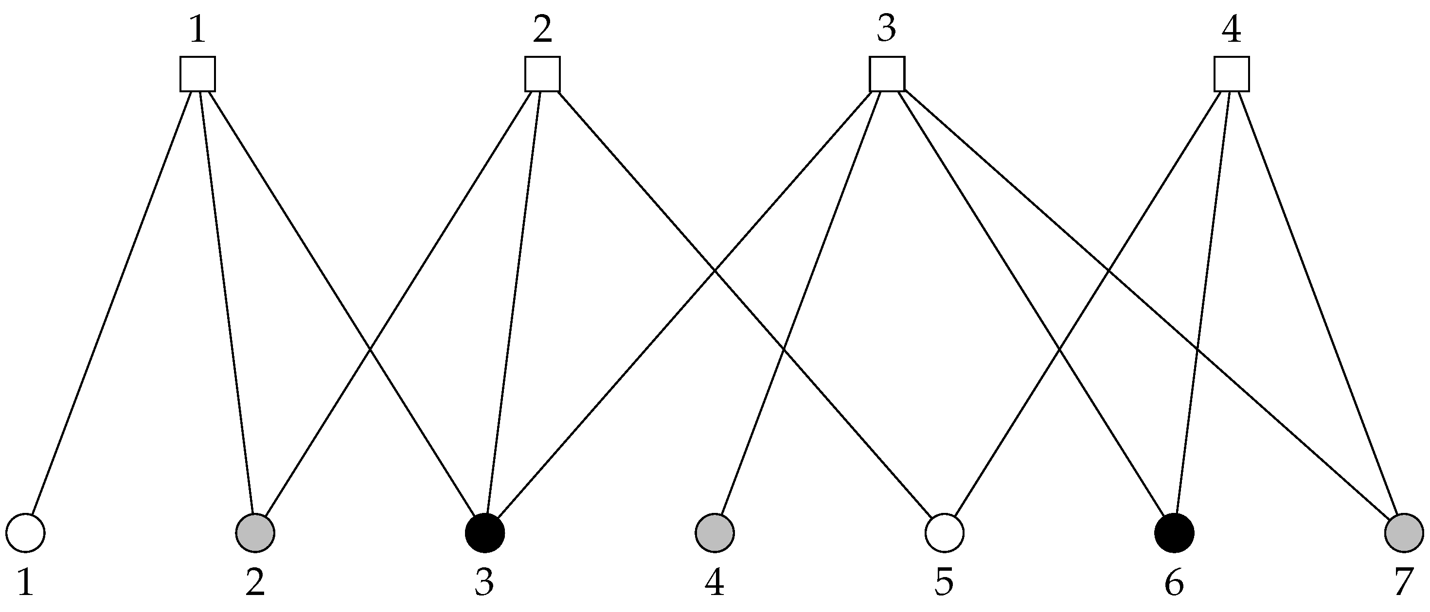
Figure 1 provides an intuitive illustration of the G-MCLP/G-PSCLP, where the red, green, and blue points represent demand points with coverage requirements of 3, 2, and 1, respectively, and the triangles denote potential facility locations with a circular service radius. A more detailed and fundamental illustration of both problems is provided by Figure 2. In Figure 2, we illustrate an example involving four facilities (represented by squares) and seven demand points (represented by circles). Each edge indicates that the corresponding facility is capable of covering the connected demand point. Specifically, white, gray, and black circles represent demand points with coverage requirements of one, two, and three, respectively. In the context of the G-MCLP/PSCLP, demand point 3 requires service by three facilities and is therefore considered satisfied only if facilities 1, 2, and 3 are all selected. Similarly, demand point 7 is considered covered only if both facilities 3 and 4 are selected. It is worth noting that under the classical MCLP/PSCLP setting, where each demand point requires service by at least one facility, selecting facilities 1, 3, and 4 would suffice to cover all demand points in Figure 2. In contrast, under the G-MCLP/PSCLP framework, selecting facilities 1, 3, and 4 covers only demand points 1, 5, and 7.
Since both the MCLP and PSCLP have been proven to be NP-hard [23,24], their generalized versions, the G-MCLP and G-PSCLP, inherit this computational complexity. A substantial body of work has been dedicated to developing approximation and heuristic algorithms for the MCLP and PSCLP. These include greedy algorithms [13], Lagrangian relaxation techniques [25], partial constraint relaxation methods [26], instance reduction strategies [27], genetic algorithms [28], and guided adaptive search algorithms [29] for the MCLP, as well as Lagrangian relaxation [14] and tabu search heuristics [30] for the PSCLP. More recently, extensions of the MCLP have been investigated from different perspectives. For instance, Lin and Tseng [31] addressed maximal coverage problems with routing constraints and proposed a cross-entropy-based Monte Carlo tree search that outperforms benchmark approaches in spatial search tasks. In parallel, Alosta et al. [32] explored a multi-criteria decision-making approach for emergency medical service location selection in Libya, integrating the Analytic Hierarchy Process (AHP) to identify the optimal site. Extending the PSCLP framework, Li et al. [33] developed differentially private approximation algorithms for facility location, thereby connecting coverage relaxation with privacy-preserving combinatorial optimization. In addition to heuristic methods, exact solutions to the MCLP/PSCLP are often obtained by formulating the problems as integer programming (IP) models and solving them using general-purpose solvers [13,34]. The computational efficiency of such IP formulations has been further enhanced through techniques such as presolving [35] and decomposition-based strategies, including branch-and-Benders-cut reformulations [36]. It is worth noting that the branch-and-Benders-cut reformulation effectively separates the coverage constraints in the MCLP/PSCLP models, incorporating them dynamically during the solution process only when necessary. This reformulation substantially improves computational efficiency, enabling the exact solution of instances with tens of thousands of demand points in a more timely manner, thus better reflecting real-world problem sizes. However, when extended to the G-MCLP/PSCLP, where each demand point must be covered by multiple facilities, these methods become inapplicable due to the inherent complexity introduced by the multi-coverage requirement. For a broader overview of research on covering problems, the reader is referred to two comprehensive survey articles [37,38].
To address reliability considerations in facility location planning, the G-MCLP was first explicitly formulated as a probabilistic extension of the classical MCLP by ReVelle and Hogan [39], known as the Maximal Availability Location Problem (MALP). In the MALP, the probability that a demand point is effectively served increases with the number of covering facilities. To ensure that this probability exceeds a predefined threshold, each demand point is assigned a fixed coverage requirement, thereby giving rise to the G-MCLP. Since then, the G-MCLP has frequently been embedded as a subproblem within probabilistic or queueing-based location models [16,40,41]. In these studies, the G-MCLP is typically modeled as an IP and solved directly using general-purpose solvers, which limits scalability to instances with fewer than 100 demand points. This computational bottleneck has significantly constrained progress in related research. To the best of our knowledge, no existing study has investigated exact algorithmic acceleration techniques for the G-MCLP [42]. Moreover, its dual counterpart, the G-PSCLP, has not yet been formally introduced in the literature.
Although no existing study has explicitly focused on developing efficient exact algorithms for solving the G-MCLP/PSCLP, several related problems have been explored in the literature. Berman et al. [43] examined a continuous cooperative covering model, where the signal strength received by a demand point depends on its distance from the serving facilities. Specifically, closer facilities provide stronger signals, and the signal contributions from multiple facilities are additive. If the signal strength received by a demand point is assumed to be constant for facilities capable of serving it, then the model reduces to the G-MCLP/PSCLP. In their study, a variety of classical solution techniques commonly used for MCLP- and PSCLP-type problems were investigated, including Lagrangian relaxation, the ascent algorithm, simulated annealing, tabu search, and genetic algorithms. However, these approaches are heuristic or approximation algorithms and do not guarantee optimality. Curtin et al. [19] incorporated the concept of multiple coverage for high-priority demand points through a multi-objective optimization framework. In contrast to the hard coverage requirements imposed in the G-MCLP/PSCLP, their model first ensured that all demand points were covered by at least one facility and then sought to provide additional coverage for high-priority demand points whenever possible. They adopted the classical constraint method in multi-objective optimization, which resulted in a set of Pareto-optimal solutions that balance maximal coverage with redundant coverage.
Despite the wide range of practical applications and growing demand for the G-MCLP/PSCLP, effective exact solution methods for these generalized models remain largely underdeveloped. To bridge this gap, this paper proposes efficient exact algorithms that are specifically designed to exploit the structural characteristics of the G-MCLP/PSCLP. The main contributions of this work are summarized as follows:
  • We generalize and formulate IP models for the classical MCLP/PSCLP by incorporating a multiple coverage requirement, whereby each demand point must be served by a specified number of facilities. This extension significantly broadens the applicability of these models to real-world scenarios with stringent reliability requirements;
  • We reformulate the generalized models to enhance their structural properties. In particular, the reformulation allows variables associated with demand point coverage to be relaxed as continuous without altering the optimal solution. This property facilitates the use of decomposition techniques and helps reduce the overall computational burden;
  • Building on the reformulated models, we develop exact Benders decomposition algorithms that dynamically introduce violated constraints as needed for both problems. Moreover, we design efficient separation algorithms and establish their time and space complexity bounds. The algorithms effectively exploit problem structures and yield substantial improvements in scalability and computational efficiency;
  • Computational experiments show that the proposed method achieves superior efficiency compared to state-of-the-art solvers on instances with up to 200,000 demand points as well as on real-world cases. Furthermore, our method outperforms the tabu search heuristic by obtaining higher-quality feasible solutions.
The remainder of this paper is organized as follows. Section 2 formally defines the G-PSCLP/MCLP, presenting their IP formulations and highlighting key differences from classical models. Section 3 presents exact solution methodologies for the proposed problems, building on model reformulation and the branch-and-Benders-cut approach. Section 4 details the branch-and-Benders-cut implementation framework, featuring an efficient separation procedure for dynamically generated cuts. Section 5 comprehensively evaluates computational performance through extensive experiments on synthetic and real-world datasets, benchmarking against both state-of-the-art IP solvers and a tabu search heuristic. Finally, Section 6 summarizes key findings and suggests promising research directions.

2. Problem Formulation

In this section, we formally define the two previously introduced problems, the G-MCLP/PSCLP, and present their mathematical formulations.
Consider a set of potential facility locations I = { 1 , 2 , , | I | } and a set of demand points J = { 1 , 2 , , | J | } . Each potential facility location i I is associated with a construction cost f i . Each demand point j J is characterized by two parameters, (i) a demand value d j 0 and (ii) a coverage requirement M j Z + , such that M j | I ( j ) | , where I ( j ) I denotes the set of facility locations capable of covering demand point j.
The problem is formulated using two sets of binary decision variables: y { 0 , 1 } | I | and z { 0 , 1 } | J | , corresponding to potential facility locations and demand points, respectively. The value of y i = 1 for i I indicates that facility i is selected; otherwise, y i = 0 . Similarly, z j = 1 for j J indicates that demand point j is sufficiently covered; in other words, it is covered by at least M j facilities in I ( j ) .
Given a budget parameter B > 0 , the G-MCLP seeks to maximize the total value of covered demand points, subject to a facility budget constraint. It can be formulated as the following IP model [41]:
max y , z j J d j z j
s . t . i I ( j ) y i M j z j , j J ,
i I f i y i B ,
y { 0 , 1 } | I | ,
z { 0 , 1 } | J | .
The objective function (1) maximizes the total covered value of demand points. Constraint (2) establishes that demand point j is considered covered ( z j = 1 ) only when at least M j facilities capable of serving it are opened. Constraint (3) ensures that the total cost of opened facilities does not exceed the available budget B.
Conversely, the G-PSCLP represents a symmetric counterpart to the G-MCLP, aiming to minimize the total cost of the selected facilities while ensuring that the total value of sufficiently covered demand points exceeds a given coverage threshold D > 0 . Using the same set of decision variables as in the G-MCLP, the G-PSCLP can be formulated as follows:
min y , z i I f i y i
s . t . j J d j z j D , ( 2 ) , ( 4 ) , ( 5 ) .
In the G-PSCLP the objective function (6) minimizes the total facility opening cost. Constraint (7) ensures that the total value of covered demand points is at least D. Constraints (2), (4), and (5) mirror their counterparts in the G-MCLP formulation. Compared to the G-MCLP, we observe that the objective function and the facility budget constraint are interchanged such that the objective function defined in (6) now minimizes the facility construction cost, while the constraint (7) ensures that the total value of demand points meets a minimum threshold. Compared to the classical MCLP/PSCLP [13,14], the difference in the G-MCLP/PSCLP lies in constraint (2). In the classical models, the counterpart is given by
i I ( j ) y i z j , j J ,
which can be seen as a special case of generalized model when M j = 1 for all j J .
In practical applications, the massive number of demand points often renders standard MIP solvers inefficient, even during the linear relaxation phase. To address this challenge, Cordeau et al. [36] studied an effective decomposition approach for the MCLP/PSCLP (i.e., the G-MCLP/PSCLP with M j = 1 , j J ) based on a branch-and-Benders-cut reformulation. They first relaxed the binary coverage variables z to continuous variables in the interval [ 0 , 1 ] | J | , which enabled the application of classical Benders decomposition by ensuring that the subproblems remained a linear program. Subsequently, they derived several closed-form expressions for generating valid Benders cuts from the subproblem. However, this Benders decomposition procedure faces significant difficulties when extended to the G-MCLP/PSCLP models. In these generalized models, the coefficient of z j in constraint (2) changes from 1 to M j , which breaks the integrality relaxation property. As explained in Remark 1 below, relaxing the z -variables under these conditions can lead to an incorrect optimal solution, thereby preventing the direct application of the Benders decomposition method.
Remark 1. 
Relaxing the integrality of z in the G-MCLP/PSCLP may lead to a change in the optimal value. We illustrate this phenomenon using the G-MCLP model below; the argument for G-PSCLP is analogous.
max y , z z 1 + z 2 s . t . y 1 + y 2 4 z 1 , y 1 + y 2 z 2 , y 1 + y 2 2 , ( y 1 , y 2 ) { 0 , 1 } 2 , ( z 1 , z 2 ) { 0 , 1 } 2 .
The optimal solution to (9) is ( y 1 , y 2 , z 1 , z 2 ) = ( 1 , 1 , 0 , 1 ) , yielding an objective value of 1. However, if z 1 and z 2 are relaxed to the continuous domain [ 0 , 1 ] , the optimal solution becomes ( y 1 , y 2 , z 1 , z 2 ) = ( 1 , 1 , 0.5 , 1 ) , with an objective value of 1.5 . This demonstrates that relaxing the integrality of z can lead to a change in the optimal value of the G-MCLP.
The next section begins with reformulations of the G-MCLP/PSCLP models and then introduces an efficient branch-and-Benders-cut framework to solve them.

3. Exact Solution Methods for G-MCLP and G-PSCLP

This section presents exact solution methods for the G-MCLP/PSCLP. We first reformulate the original models to improve their structural properties and facilitate decomposition. Based on these formulations, Benders decomposition algorithms are developed to efficiently solve the reformulated problems.

3.1. Problem Reformulation

In the following, we reformulate the G-MCLP/PSCLP models by introducing a new set of inequalities. The resulting formulations are equivalent to the original ones but feature structures that are more amenable to Benders decomposition. This development is based on a detailed analysis of constraints (2), which is formalized in the proposition below.
Proposition 1. 
The feasible set
X = { ( y , z ) : ( 2 ) , ( 4 ) , ( 5 ) }
is equivalent to
X = { ( y , z ) : ( 10 ) , ( 4 ) , ( 5 ) } ,
where constraint (10) is defined as follows:
i H y i z j , H H j , j J ,
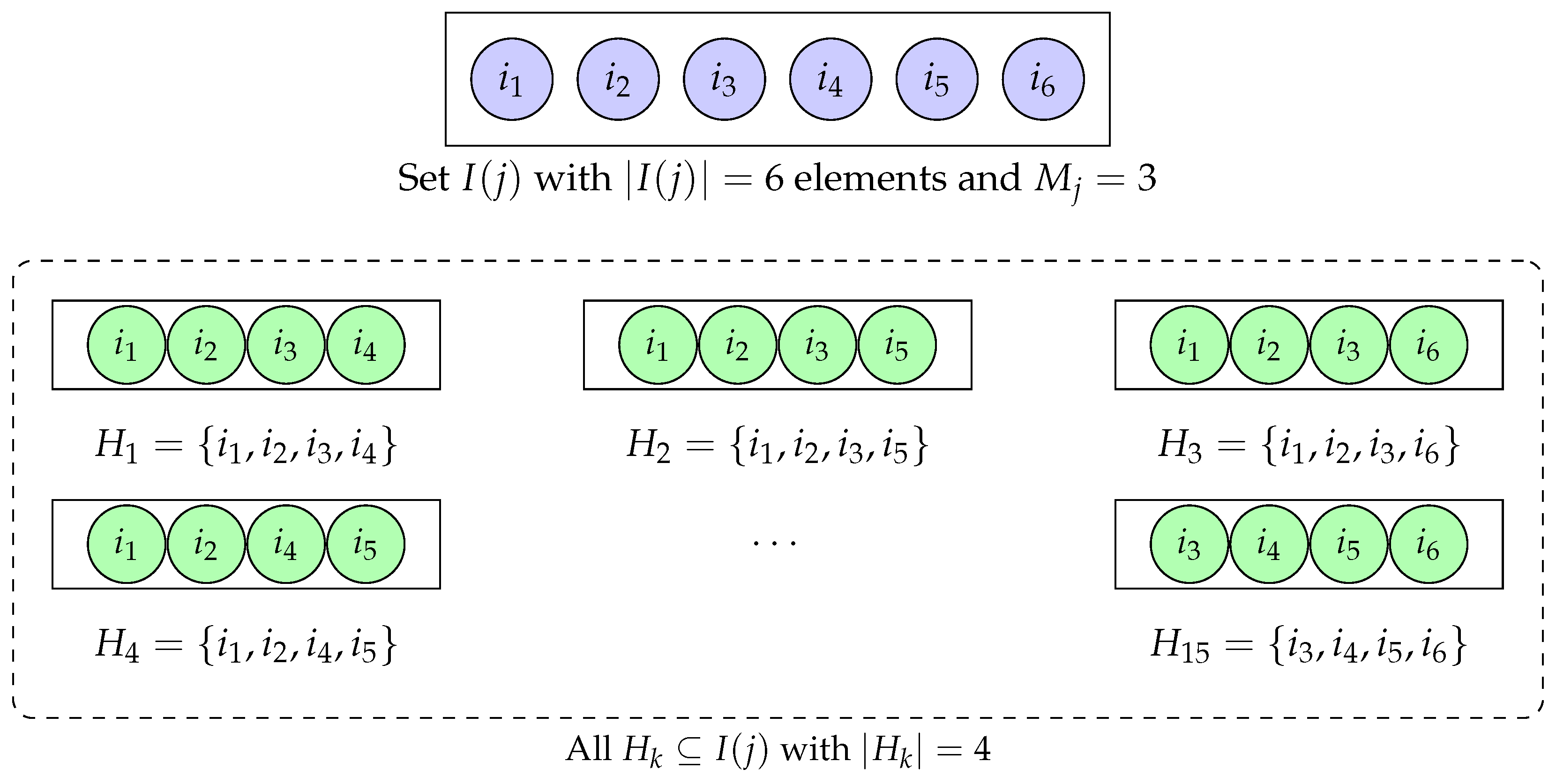
with H j = { H I ( j ) : H = I ( j ) M j + 1 } (see Figure 3 for an illustration).
Proof of Proposition 1. 
It suffices to show that all ( y , z ) { 0 , 1 } | I | + | J | satisfying either (2) or (10) also satisfy the other. The proof is therefore divided into two parts:
  • We first show that for any j J , if ( y , z ) satisfies i I ( j ) y i M j z j , then it also satisfies i H y i z j , H H j . When z j = 0 , the inequality i H y i z j trivially holds for all H H j . Now consider the case where z j = 1 . Then, we have
    i I ( j ) y i M j .
    Since y { 0 , 1 } | I | , this implies that no more than | I ( j ) | M j components of y i : i I ( j ) can be equal to 0. Therefore, any subset of I ( j ) containing at least I ( j ) M j + 1 elements must include at least one i with y i = 1 . That is
    i H y i 1 = z j , H H j .
  • Conversely, for any j J , assume that ( y , z ) satisfies i H y i z j for all H H j . If z j = 0 , the inequality i I ( j ) y i 0 trivially holds. Now suppose z j = 1 . Take any H 1 H j . Since i H 1 y i 1 , there exists at least one index i 1 H 1 I ( j ) such that y i 1 = 1 . Next, consider another subset H 2 H j such that H 2 I ( j ) { i 1 } . Similarly, we can find i 2 H 2 such that y i 2 = 1 . Repeat this process over subsets H 3 I ( j ) { i 1 , i 2 } , H 4 I ( j ) { i 1 , i 2 , i 3 } , and so on. After M j steps, it leads to set H M j , which is non-empty as | I ( j ) | M j . As a result, we obtain M j distinct indices { i 1 , i 2 , , i M j } I ( j ) for which y i k = 1 for all k { 1 , , M j } . This implies that i I ( j ) y i M j , which completes the proof.    □
Proposition 1 shows that, for each demand point j J , the condition that it is covered by at least M j facilities is equivalent to requiring that every subset H I ( j ) of cardinality | I ( j ) | M j + 1 contains at least one open facility. By replacing the original formulation involving X with its equivalent counterpart X , equivalent reformulations of the G-MCLP/PSCLP models are naturally obtained:
G-MCLP:
max y , z j J d j z j : ( 10 ) , ( 3 ) , ( 4 ) , ( 5 ) .
G-PSCLP:
min y , z i I f i y i : ( 10 ) , ( 7 ) , ( 4 ) , ( 5 ) .
For any j J , each constraint from (2) in the original model corresponds to | I ( j ) | M j + 1 | I ( j ) | constraints from (10) in the reformulated model, where · · denotes the binomial coefficient. As a result, the reformulated models have a significantly larger number of constraints compared to the original ones. However, as established in Proposition 2, the latter formulation permits the relaxation of variables z to continuous values in [ 0 , 1 ] | J | without altering the optimal solution.
Proposition 2. 
In the reformulated G-MCLP/PSCLP models (11) and (12), the integrality conditions (5) can be relaxed to z [ 0 , 1 ] | J | without changing the optimal values.
Proof of Proposition 2. 
Let ( y , z ) { 0 , 1 } | I | × [ 0 , 1 ] | J | be an optimal solution to model (11) or (12), where the integrality constraint on z is relaxed.
To begin with, consider the G-MCLP model. Suppose there exists some j J such that z j ( 0 , 1 ) . Since y is binary, the left-hand side of constraint (10) corresponding to z j , i.e., i H y i , H H j , must be at least 1. Therefore, setting z j = 1 still satisfies constraint (10) and yields a feasible solution. Moreover, since d j 0 , replacing z j ( 0 , 1 ) with 1 does not decrease the objective value. Thus, the modified solution remains feasible and achieves an objective value at least as good as the relaxed solution. It follows that the relaxed problem always admits an optimal solution in which all variables are integral, which in turn implies that its optimal value coincides with that of the original problem. Similarly, for the G-PSCLP, the modified integer solution obtained by rounding up the fractional values in z remains feasible for the relaxed problem and achieves the same objective value. This completes the proof.    □
Remark 2. 
For both the G-MCLP/PSCLP, when the integrality constraints on z are relaxed, there exists an optimal solution ( y , z ) such that z can be expressed as a function of y :
z j = min min H H j i H y i , 1 , j J .
Indeed, as shown in the proof of Proposition 2, any optimal solution can be transformed into another optimal and feasible solution by rounding up all fractional z variables in the interval ( 0 , 1 ) . Therefore, the resulting solution satisfies the expression above.
Remark 3. 
There is no dominance relationship between the original and the reformulated models in terms of the tightness of their LP relaxations. We illustrate this observation with two examples: max z , y 1 , y 2 , y 3 [ 0 , 1 ] { z : y 1 + y 2 + y 3 2 z , y 1 + y 2 + y 3 2 } and max z , y 1 , y 2 , y 3 [ 0 , 1 ] { z : y 1 + y 2 z , y 1 + y 3 z , y 2 + y 3 z , y 1 + y 2 + y 3 2 } . The point ( z , y 1 , y 2 , y 3 ) = 0.25 , 0.5 , 0 , 0 is feasible for the former but infeasible for the latter, whereas the point ( z , y 1 , y 2 , y 3 ) = 0.2 , 0.1 , 0.1 , 0.1 is feasible for the latter but infeasible for the former. A similar observation holds for the G-PSCLP, which we omit here.
However, it is worth noting that for any j J , if M j = | I ( j ) | (which means that the demand point is considered covered only when all facilities capable of serving it are selected), then constraint (10) reduces to y i z j , i I ( j ) . By summing these inequalities, one can recover the corresponding constraint in (2). Therefore, in this case, the LP relaxation of the reformulated model is at least as strong as that of the original model.

3.2. Benders Decomposition for G-MCLP

This section outlines a Benders separation algorithm designed for the G-MCLP. In the following, we first derive the Benders optimal inequalities for the G-MCLP in Section 3.2.1. Then we show that the Benders inequalities can be efficiently separated in Section 3.2.2.

3.2.1. Benders Optimality Inequalities

According to Section 3.1, relaxing the integrality constraints on z in (11) yields an equivalent formulation of the G-MCLP model as follows.
max y , z j J d j z j : ( 10 ) , ( 3 ) , ( 4 ) , z [ 0 , 1 ] | J | .
As observed from Remark 2, the optimal values of variables z can be computed as a function of y explicitly in formulation (13). This enables us to propose a linear way to project out variables z and develop a Benders decomposition approach to solve the G-MCLP/PSCLP. Since the variables z appear in the objective function, Benders optimality cuts are introduced, and the value of the objective function is modeled using an auxiliary variable θ 0 . To begin with, we project out variables z and obtain the Benders master problem:
max y , θ θ : ( 3 ) , ( 4 ) , B t ( y , θ ) 0 , t P ,
where B t ( y , θ ) refers to Benders optimality inequalities corresponding to extreme points t of the polyhedron P. Here, P denotes the feasible region of the LP dual of the Benders subproblem, and we derive its explicit formulation below.
Given a fixed y ¯ [ 0 , 1 ] | I | , the corresponding Benders subproblem is formulated as follows:
max z j J d j z j : Σ ¯ H z j , H H j , z [ 0 , 1 ] | J | ,
where Σ ¯ H = i H y ¯ i . Observe that the Benders subproblem (15) is always feasible, since the all-zero vector is a feasible solution. We only need to introduce the Benders optimality cuts. The dual-symmetric version of the Benders subproblem (15) can be obtained by introducing (i) dual variables π j , H associated with constraint i H y ¯ i z j for each j J and H H j and (ii) the dual variable δ j associated with constraint z j 1 for each j J :
min π , δ j J H H j π j , H Σ ¯ H + j J δ j : ( π , δ ) P ,
where P = { ( π , δ ) 0 : H H j π j , H + δ j d j , j J } .
From LP duality theory, we know that the Benders subproblem (15) and its dual (16) share the same optimal value. Then, for any extreme point t = ( π ¯ , δ ¯ ) of the dual feasible region P, the associated Benders optimality inequality can be written as follows:
j J H H j π ¯ j , H i H y i + δ ¯ j θ 0 .
Enumerating all extreme points of P is impractical due to their exponential number. However, not all Benders optimality inequalities are necessary to obtain the optimal solution of formulation (14). To address this, we adopt the well-established branch-and-Benders-cut framework, which solves the problem efficiently by iteratively refining a relaxed Benders master problem that initially includes only a subset of the inequalities (17). A single enumeration tree is then constructed based on the relaxed master problem, and Benders cuts are dynamically generated and added during the solution process for both integer and fractional solutions encountered in the standard branch-and-cut procedure. We will provide a more detailed description of the branch-and-Benders-cut strategy in Section 4. For comprehensive discussions of the branch-and-Benders-cut approach applied to various problems, we refer the readers to Fischetti et al. [44], Cordeau et al. [36], and Güney et al. [45]. The efficiency of the Benders cut separation is critical to the overall computational performance. In the next subsection, we introduce an effective separation algorithm for the Benders optimality cuts.

3.2.2. Separation of Benders Optimality Inequalities

For a solution ( y ¯ , θ ¯ ) [ 0 , 1 ] | I | × R + of the relaxed Benders master problem, the objective of the separation problem is to either identify a violated inequality of the form (17) at the point ( y ¯ , θ ¯ ) or to certify that no such inequality exists. In other words, by fixing y = y ¯ and solving problem (16), if the resulting objective value is less than θ ¯ , a violated Benders cut is obtained; otherwise, the current solution is optimal. Problem (16) can be decomposed into | J | subproblems, each associated with a facility j J and involving only the variables δ j and π j , H for all H H j . Each subproblem takes the following form:
min π , δ H H j Σ ¯ H π j , H + δ j : H H j π j , H + δ j d j .
Problem (18) is a standard linear program with a single constraint. Let H ˜ j = arg min H H j Σ ¯ H . Then, the optimal solution ( π j , δ j ) R + | H j | + 1 , j J can be explicitly given as follows:
π ˜ j , H ˜ j , δ ˜ j = ( d j , 0 ) , if Σ ¯ H ˜ j 1 ( 0 , d j ) , if Σ ¯ H ˜ j > 1 π ˜ j , H = 0 , H H j { H ˜ j } .
Then, if
j J H H j π ˜ j , H Σ ¯ H + δ ˜ j < θ ¯ ,
the violated Benders optimality cut can be derived as follows:
j J H H j π ˜ j , H i H y i + δ ˜ j θ .
Otherwise, the current solution is optimal for the original problem (13), and the separation procedure terminates.
In terms of computational complexity, for a relaxed solution ( y ¯ , θ ¯ ) , the separation problem requires solving H ˜ j = arg min H H j Σ ¯ H for all j J . Since H j denotes all subsets of I ( j ) with cardinality | I ( j ) | M j + 1 , the set H j is exponential in size. However, the minimization can be obtained by simply selecting the | I ( j ) | M j + 1 smallest elements of I ( j ) . Hence, the separation reduces to sorting I ( j ) , which requires O ( | I ( j ) | log | I ( j ) | ) time. Summing over all demand points, the overall complexity is bounded by O ( | J | | I | log | I | ) . In terms of space complexity, since the | J | subproblems are solved sequentially and each subproblem only requires the storage of I ( j ) for the sorting procedure, the space complexity of the separation algorithm is O ( | I | ) . In practice, since each facility typically covers only a small subset of the total demand points, the actual computational and space costs are considerably lower than this worst-case bound.
Remark 4 
([36]). It deserves to be mentioned that, if H ˜ j contains only one element and Σ ¯ H ˜ j = 1 for some j J , setting π ¯ j , H ˜ j , δ ¯ j = ( d j , 0 ) can result in a stronger Benders cut. This is because, under these conditions, the j-th term of the Benders cut (21) becomes π ˜ j , H ˜ i H ˜ y i + δ ˜ j = π ˜ j , H ˜ y i 0 + δ ˜ j , where H ˜ = { i 0 } . Since y i 0 1 , the choice π ¯ j , H ˜ j , δ ¯ j = ( d j , 0 ) leads to a dominating cut compared to the alternative setting π ¯ j , H ˜ j , δ ¯ j = ( 0 , d j ) . In addition, when Σ ¯ H ˜ j = 1 , one has the freedom to set either π ¯ j , H ˜ j , δ ¯ j = ( d j , 0 ) or ( 0 , d j ) in (19), as neither choice strictly dominates the other. Our preliminary computational experiments indicate that setting π ¯ j , H ˜ j , δ ¯ j = ( d j , 0 ) tends to yield better performance in such cases.
Remark 5. 
In the separation problem described above, the computation of each H ˜ j is mutually independent, which allows for the use of parallel computation. However, as this is not the main focus of the present study, we do not pursue its discussion or implementation here.

3.3. Benders Decomposition for G-PSCLP

The Benders separation algorithm for the G-PSCLP closely mirrors that of the G-MCLP. Section 3.3.1 outlines the derivation of Benders feasible inequalities, while Section 3.3.2 details the associated separation method. For the G-PSCLP, a normalization technique [36] is employed to achieve the same level of separation efficiency as in the G-MCLP.

3.3.1. Benders Feasibility Inequalities

Similarly, by relaxing the variables z to continuous in (12), we obtain the following formulation of the G-PSCLP model suitable for Benders decomposition.
min y , z i I f i y i : ( 10 ) , ( 7 ) , ( 4 ) , z [ 0 , 1 ] | J | .
Unlike the G-MCLP, the G-PSCLP can be fully characterized using only Benders feasibility cuts, owing to the absence of z in the objective function. Next, we project out z and obtain the Benders master problem:
min y i I f i y i : B q ( y ) 0 , q Q , y { 0 , 1 } I ,
where B q ( y ) refers to Benders feasibility inequalities corresponding to extreme rays q of the polyhedron Q associated with the LP dual of the Benders subproblem. The Benders subproblem with y ¯ [ 0 , 1 ] | I | reads as follows:
min z 0 : Σ ¯ H z j , H H j , z [ 0 , 1 ] | J | , j J d j z j D ,
where Σ ¯ H = i H y ¯ i . By introducing (i) dual variables π j , H associated with constraint Σ ¯ H z j for each j J and H H j , (ii) dual variable δ j associated with constraint z j 1 for each j J , and (iii) dual variable γ associated with constraint j J z j D , the dual-symmetric formulation of (24) is given by
max π , δ , γ j J H H j ( Σ ¯ H ) π j , H j J δ j + D γ : ( π , δ , γ ) Q ,
where Q = { ( π , δ , γ ) 0 : H H j π j , H δ j + d j γ 0 , j J } .
From LP duality theory we know that the primal subproblem is infeasible if and only if its dual is unbounded. Then for any extreme ray q = ( π ¯ , δ ¯ , γ ¯ ) of Q , the associated Benders feasibility inequality can be written as follows:
j J H H j π ¯ j , H i H y i + δ ¯ j D γ ¯ 0 .
In a similar manner, the problem is solved by iteratively refining a relaxed master problem that initially contains only a subset of the Benders inequalities under a branch-and-Benders-cut framework detailed in Section 4. An effective separation algorithm for the Benders feasibility cuts (26) is presented in the following subsection.

3.3.2. Separation of Benders Feasibility Inequalities

Let y ¯ [ 0 , 1 ] | I | be a solution of the Benders relaxed master problem. Observe that, if γ = 0 , then it follows the fact that both ( y ¯ , z ¯ ) and ( π ¯ , δ ¯ , γ ¯ ) have non-negative values and that Benders feasibility inequality (26) cannot be violated by ( y ¯ , z ¯ ) . As a result, in order to obtain a violated Benders feasibility inequality that cuts off point ( y ¯ , z ¯ ) , it is sufficient to enforce γ > 0 in (25). Without loss of generality, we can normalize γ = 1 , and rewrite problem (25) as follows:
max π , δ D j J H H j Σ ¯ H π j , H + δ j : H H j π j , H + δ j d j , j J .
Notice that problem (27) is in fact equivalent to problem (19). Therefore, the time complexity of the separation problem is bounded by O ( | J | | I | log | I | ) , while the space complexity is O ( | I | ) . For any j J , the explicit solution is given by (19). Then, if
j J H H j π ¯ j , H Σ ¯ H + δ ¯ j < D ,
the violated Benders feasibility cut can be derived as follows:
j J H H j π ¯ j , H i H y i + δ ¯ j D ,
Otherwise, the current solution is optimal.

4. Branch-And-Benders-Cut Strategy

This section is devoted to our Benders decomposition strategy for solving the G-MCLP/PSCLP. The corresponding pseudocode is provided in Algorithm 1.
For the G-MCLP, rather than solving the full model (14) with all constraints from the outset, we adopt a row generation approach within a branch-and-bound framework [46,47]. Specificity, except for the budget constraint (3) and binary restrictions on variables (4), all Benders optimality cuts are added lazily; that is, they are incorporated into the master problem only when violated by the current relaxed solution encountered during the search.
The Benders decomposition algorithm generates Benders optimality cuts following the procedure outlined in Section 3.2.2. For each demand point variable y j , j J , note that in (18), the dual variables π ˜ j , H corresponding to all H H j H ˜ j are zero. Therefore, the Benders optimality cut (21) can be expressed in the following simplified form:
j J π ˜ j , H ˜ j i H ˜ j y i + δ ˜ j θ .
Hence, it suffices to focus on the | H ˜ j | elements in I ( j ) with the smallest relaxed values and compute Σ ¯ H ˜ j accordingly. This can be efficiently achieved using a sorting algorithm with time complexity O ( | I ( j ) | log | I ( j ) | ) .
Similarly to the case of the G-MCLP, for the G-PSCLP model, we implement the formulation proposed in (23) by dynamically separating the constraints in (26) within a branch-and-cut framework. In contrast to the G-MCLP, since the objective function of (23) does not involve the variable z , Benders optimality cuts are not required. The generation of Benders feasibility cuts follows the separation procedures detailed in Section 3.3.2. Notably, since problem (27) is equivalent to problem (19), and the only difference between (29) and (21) lies in the right-hand-side term, with D in the former and θ in the latter, the procedure for generating Benders feasibility cuts in the G-PSCLP is operationally identical to that for generating Benders optimality cuts in the G-MCLP.
Algorithm 1 Branch-and-Benders-cut strategy
Require:
               G-MCLP:   The IP model (14), and the current LP relaxed solution ( y , θ ) [ 0 , 1 ] | I | × R +
               G-PSCLP: The IP model (23), and the current LP relaxed solution y [ 0 , 1 ] | I |
Ensure:
               G-MCLP:   The Benders inequalities j J a j y j θ r h s violated by ( y , θ )
               G-PSCLP: The Benders inequalities j J a j y j r h s violated by y
  1:
Initialize the Benders inequalities j J a j y j θ r h s for G-MCLP
( j J a j y j r h s for G-PSCLP) with a j = 0 for all j J and rhs = 0 .
  2:
for j J do
  3:
    Sort { y s } s I ( j ) such that y s 1 y s 2 y s | I ( j ) | ;
  4:
    Compute Σ ¯ H ˜ j = i = 1 | I ( j ) | M j + 1 y s i ;
  5:
    if  Σ ¯ H ˜ j < 1  then
  6:
       for  i = 1 , 2 , . . . , ( | I ( j ) | M j + 1 )  do
  7:
           Set a s i = a s i + d j ;
  8:
       end for
  9:
    else if Σ ¯ H ˜ j > 1 then
10:
        Set r h s = r h s d j ;
11:
    else
12:
        // Σ ¯ H ˜ j = 1
13:
        if | I ( j ) | M j + 1 = 1  then
14:
            Set a s 1 = a s 1 + d j ;
15:
        else
16:
            Set r h s = r h s d j ;
17:
        end if
18:
    end if
19:
end for

5. Computational Study

In this section, we conduct computational experiments to evaluate the proposed branch-and-Benders-cut strategy for the G-MCLP and G-PSCLP within the branch-and-bound framework of IBM CPLEX 20.1.0 [48]. All algorithms were implemented in C++, and the implementation (version 1.1.0) has been made publicly available on GitHub at https://github.com/lostedsailor/julymtpu (accessed on 23 August 2025). CPLEX’s callback functions were employed to add lazy constraints and user cuts. The relative gap tolerance was set to 0 % , and each run was carried out in single-threaded mode. To ensure comparability and stability in both problem size and structure, preprocessing in CPLEX was disabled for both the experimental and baseline settings. All other parameters were kept at their default values. The experiments were performed on a 64-bit Linux cluster equipped with 2.30 GHz Intel(R) Xeon(R) Gold 6140 CPUs and 180 GB of RAM.

5.1. Results and Analysis of Random Instances

Our testbed of instances is constructed with reference to ReVelle et al. [27] and Cordeau et al. [36], where randomly generated instances of the G-MCLP/PSCLP were introduced. In all test instances, the geographical area is defined as a 30 × 30 square grid, where the coordinates of each demand point and potential facility location are independently drawn from a uniform distribution over the continuous interval [ 0 , 30 ] . The values of demand points are randomly generated as integers in the interval [ 1 , 100 ] . In line with real-world scenarios where the construction cost of facilities is often identical, we set f i = 1 for all i I . For each potential facility location i, the set J ( i ) includes all demand points whose Euclidean distance from location i is less than the facility coverage radius R. Similarly, for each demand point j, the set I ( j ) contains all potential facilities within its radius that can cover it. The coverage requirement M j for each demand point j is randomly selected as an integer from the interval [ 1 , 10 ] . For the G-MCLP instances, we set the facility budget constraint to B { 10 , 15 , 20 } . For the G-PSCLP instances, the covering demand D is defined as a percentage of the covering demand D ¯ = j J d j , with D { 50 % D ¯ , 60 % D ¯ , 70 % D ¯ } . For each combination of input parameters, we generate ten instances with identical characteristics, varying only the random seed used for data generation. As highlighted in the introduction, our exact approach is specifically designed for realistic scenarios where the number of demand points far exceeds the number of potential facility locations, i.e., | J | | I | . Accordingly, we fix the number of facility locations at | I | = 100 , while varying the number of demand points | J | between 30,000 and 70,000. Table 1 summarizes the main parameter settings used for generating test instances.
We next compare the performance of our branch-and-Benders-cut framework based on Algorithm 1, denoted as BEN in the tables, against the direct use of CPLEX applied as a black-box solver, denoted as CPX in the tables, on the compact formulations (1)–(7).
In Table 2 and Table 3, we present the performance comparison results for the G-MCLP and G-PSCLP, respectively. We consider all benchmark instances with the number of demand points set to {30,000, 50,000, 70,000}. Each row in the tables reports the average computing time required to solve instances with similar characteristics, grouped by increasing values of covering demand D (for the G-PSCLP) and budget B (for the G-MCLP). “#” denotes the total number of test instances in each row. For each algorithm, we report the number of instances in each group that were solved to proven optimality (column “# opt”) for each group. Average CPU times are computed under a time limit of 1000 s. For instances not solved within the time limit, the computing time is recorded as 1000 s.
For the G-MCLP instances, the results in Table 2 demonstrate that our branch-and-Benders-cut algorithm consistently outperforms CPX across all test configurations. Overall, it can be observed that the computational difficulty of solving MCLP instances increases proportionally with both the number of demand points and the facility budget. Furthermore, our method successfully solves 259 out of 270 instances to proven optimality within the time limit, achieving a success rate of 95.93%. The few unsolved instances occur primarily when the budget B = 20 , where BEN solves 79 out of 90 instances (87.78%) across all three problem sizes. In contrast, CPX demonstrates significantly inferior performance, solving only 160 instances (59.26%) within the time limit. The performance gap becomes particularly pronounced as the problem size increases—when | J | = 70,000, CPX solves only 39 out of 90 instances (43.33%), with the solve rate dropping to merely 16.67% (5 out of 30) for B = 20 . The computational efficiency advantage of BEN is equally striking. For smaller instances ( | J | = 30,000 and B = 10 ), BEN achieves solutions in just 10.79 s on average, compared to CPX’s 172.04 s—a speedup factor of nearly 16. This efficiency gap persists across all problem configurations. Even for the most challenging instances ( | J | = 70,000, B = 20 ), BEN maintains an average solving time of 335.67 s while solving 90.00% of instances, whereas CPX requires 923.67 s on average despite solving only 16.67% of instances. CPX exhibits sensitivity to increases in problem size, whereas BEN maintains a relatively stable performance. The performance profile in Figure 4 provides an intuitive illustration of the solution behavior across all 270 instances.
For the G-PSCLP instances shown in Table 3, BEN again demonstrates superior performance, and Figure 5 presents the corresponding performance profile. Similarly to the MCLP, the computational difficulty increases with both the number of demand points and the level of covering demand. The performance differential is most pronounced for large-scale problems with high coverage requirements. When | J | = 70,000 and D = 70 % D ¯ , BEN successfully solves 24 out of 30 instances (80.00%) with an average time of 490.63 s, while CPX manages only 8 instances (26.67%) with an average time of 914.20 s. BEN’s computational efficiency advantage is consistent across all problem configurations. For the smallest instances ( | J | = 30,000, D = 50 % D ¯ ), BEN requires only 12.21 s compared to CPX’s 94.88 s—a speedup factor of 7.8. This efficiency gain becomes even more pronounced as problem complexity increases. For instance, when | J | = 70,000 and D = 50 % D ¯ , BEN solves all 30 instances in an average of 25.14 s, while CPX requires 478.35 s to solve 29 instances—representing an approximately 19× speedup in solution time. The computational burden increases predictably with both the number of demand points ( | J | ) and the covering demand (D) for both methods, but BEN demonstrates markedly superior scalability.
In summary, our Benders decomposition approach achieves decisive advantages over CPX across both problem classes. For the G-MCLP, BEN solves 95.93% of instances with speedups ranging from approximately 6× to 16×, while for the G-PSCLP, it achieves a 96.30% solve rate with speedups ranging from approximately 2× to 19×. The performance gap widens dramatically with increasing problem scale, confirming that our decomposition strategy effectively exploits the problem structure to maintain computational efficiency even for large-scale instances with 70,000 demand points. These results validate the practical applicability of our approach for real-world facility location problems requiring coverage redundancy.
To further evaluate the scalability of our approach, we conducted experiments on ultra-large-scale instances with up to | J | = 200,000. Under the budget settings used in the previous G-MCLP experiments and the covering demand settings in the G-PSCLP experiments, both BEN and CPX exceeded the time limit. We therefore moderately reduced the problem difficulty to enable a more informative comparison. Specifically, the budget levels in the G-MCLP were set to B { 2 , 4 , 6 } , the covering demand in the G-PSCLP was adjusted to { 10 % , 30 % , 50 % } of D ¯ , and the time limit was set to 3600 s. These settings allow us to highlight the behavior of the algorithms under extremely large-scale conditions. As reported in Table 4 and Table 5, the advantage of BEN becomes even more pronounced in this setting. The primary reason is that ultra-large-scale problems pose substantial challenges for commercial solvers, which often struggle even to compute the LP relaxation. In contrast, the dynamic constraint generation mechanism in BEN ensures that the problem remains computationally manageable throughout the iterations. Most notably, for the G-MCLP instances with | J | = 200,000, CPX fails to solve any instances to optimality at budget levels B = 4 and B = 6 , while BEN successfully solves 30 and 20 instances, respectively. Similarly, in the G-PSCLP setting with | J | = 200,000 and D = 50 % D ¯ , CPX fails across all cases, whereas BEN obtains optimal solutions for seven instances. These results demonstrate the exceptional scalability of our decomposition framework and underscore its strong potential for tackling ultra-large-scale covering location problems.
We further compared BEN with the tabu search heuristic [49] (denoted as TABU) with | I | = 100 and J {10,000, 15,000, 20,000}. Since heuristic algorithms do not guarantee convergence to optimality, we evaluated the quality of solutions obtained by both methods within a fixed time limit of 10 s. For the G-MCLP instances, larger objective values indicate better solutions, whereas for the G-PSCLP instances, smaller objective values are preferred. Each row in the tables reports the average solution quality across 30 instances. As shown in Table 6, for the G-MCLP instances with budget B = 10 , BEN and TABU achieve comparable performance. However, as the budget increases, BEN exhibits a clear advantage. This improvement can be attributed to the solver’s built-in heuristics, which, when combined with dynamically added Benders cuts, allow BEN to rapidly identify high-quality solutions during the iterative process. Similarly, Table 7 presents the results for the G-PSCLP instances. In this case, BEN consistently outperforms TABU across all settings within the same time limit, further highlighting the effectiveness of the proposed decomposition framework in guiding the search towards superior solutions.

5.2. Results and Analysis on Real-World Data

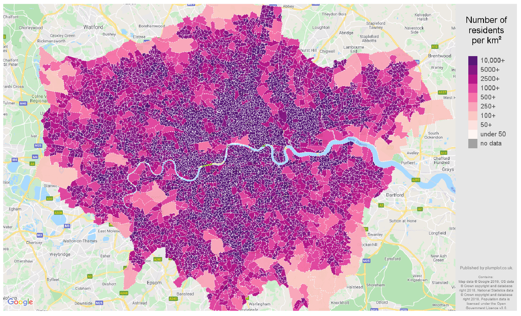
To further assess the applicability of our method to real-world problems, we employed the population distribution of London (Figure 6, data source: Plumplot https://www.plumplot.co.uk/London-population.html (accessed on 23 August 2025)) as the experimental setting. We employed a Monte Carlo sampling procedure to generate demand points according to the population density distribution, with the total number of sampled points set to 70,000. To provide a comprehensive evaluation, facility locations were randomly distributed across the map, and we tested three different scales with | I | { 80 , 100 , 120 } . The budget levels and covering demand were adopted from the ultra-large-scale experiments to ensure consistency. This setting allows us to examine the robustness and effectiveness of our approach under realistic spatial distributions.
Table 8 report the results of the G-MCLP on the real-world London population distribution. Compared with synthetic settings, the higher density and heterogeneity of demand points in this case further enlarge the problem size, posing additional challenges for exact solvers. As a result, CPX struggles to provide feasible solutions within the one-hour time limit. Specifically, with | I | = 80 facilities, CPX is able to solve fewer than 10 instances for budgets B = 4 and B = 6 . A similar pattern arises with | I | = 100 facilities and B = 4 , where the solver again fails to achieve satisfactory performance. In contrast, BEN successfully solves all instances under these settings. The scalability gap becomes even more evident when the problem size increases. For | I | = 100 facilities and B = 6 , as well as for | I | = 120 facilities with B = 4 or B = 6 , CPX fails to solve any instance within the time limit. BEN, however, remains effective across most cases, with noticeable difficulty only in the most challenging scenario of | I | = 120 and B = 6 . These results underscore the robustness of BEN in handling large-scale, real-world problems and highlight its clear advantage over state-of-the-art commercial solvers. The key factor lies in the algorithmic design: BEN dynamically incorporates constraints during the solution process, which effectively controls the growth of the model size as the problem scale increases. Consequently, the solver can maintain computational efficiency even under significantly larger instances.
For the G-PSCLP instances, Table 9 presents the results on the London population distribution. With a high covering demand of 50%, both BEN and CPX encounter severe difficulties, and feasible solutions are obtained only in a few cases (e.g., only two instances when | I | = 80 facilities). Under moderate coverage requirements (30%), BEN shows about a twofold speedup over CPX, though the advantage is less pronounced than in the G-MCLP setting. These findings demonstrate the effectiveness of BEN under moderate requirements.

5.3. Discussion

We have conducted extensive numerical experiments to comprehensively evaluate the proposed method. In addition to large-scale instances with | J | = 30,000, 50,000, and 70,000, we further tested ultra-large instances with | J | = 100,000, 150,000, and 200,000. Owing to the decomposition scheme that dynamically incorporates constraints, the effective problem size is substantially reduced. As a result, the Benders decomposition algorithm consistently demonstrates greater advantages on ultra-large instances for both the G-MCLP and the G-PSCLP. We also compared our method with a tabu search heuristic by evaluating the best feasible solutions obtained within 10 s. The experiments show that the proposed Benders decomposition approach, when embedded within CPX, consistently identifies higher-quality feasible solutions compared to the tabu search heuristic. Finally, we validated the approach on real-world data derived from the London population distribution. The dense and heterogeneous nature of demand points further increases the computational complexity. While our method maintains a clear advantage over CPX, it shows noticeable difficulty in cases with large budgets or high covering demand. This observation suggests a promising avenue for future research on further enhancing the scalability and robustness of the algorithm.

6. Conclusions

This study provided a comprehensive investigation of the G-MCLP and G-PSCLP, addressing key gaps in the literature on coverage models with redundancy requirements. We formulated generalized models that assign multi-coverage requirements to demand points, reflecting real-world reliability needs in critical applications such as emergency services and telecommunications. Novel reformulations were proposed to enable effective Benders decomposition, with theoretical guarantees that variable integrality can be relaxed without compromising optimality. Based on these reformulations, we developed tailored Benders optimality and feasibility cuts and implemented branch-and-Benders-cut algorithms.
Computational results on large-scale synthetic instances with up to 200,000 demand points demonstrate that our method achieves substantial runtime reductions compared to CPX, with performance gains becoming more pronounced as problem size increases. Moreover, a comparison with a tabu search heuristic confirms that our approach consistently delivers higher-quality solutions within short time frames, underscoring its advantages in both speed and solution quality. Finally, validation on real data from the London population density map further highlights the efficiency and robustness of the proposed method on real-world instances. Taken together, these findings demonstrate that the proposed decomposition not only achieves substantial improvements over state-of-the-art solvers on large-scale synthetic benchmarks but also scales effectively to ultra-large and real-world instances, thereby offering a promising tool for robust facility location planning.
Future research directions include designing preprocessing strategies to reduce problem size and enable the efficient solution of larger-scale instances; extending the framework to stochastic settings in which facility reliability is modeled probabilistically; incorporating capacity constraints at facilities; and developing parallel implementations to further enhance scalability. The theoretical foundations established in this study provide a solid basis for pursuing these extensions while preserving both solution quality and computational efficiency.

Author Contributions

Conceptualization, S.C.; methodology, G.L., Y.L., W.Z. and S.C.; software, G.L.; validation, G.L. and Y.L.; formal analysis, G.L., Y.L. and S.C.; investigation, G.L. and Y.L.; resources, W.Z.; data curation, Y.L.; writing—original draft preparation, G.L. and Y.L.; writing—review and editing, G.L., Y.L. and S.C.; visualization, G.L. and S.C.; supervision, S.C.; project administration, S.C.; funding acquisition, S.C. All authors have read and agreed to the published version of the manuscript.

Funding

This work was supported by the Open Project of Key Laboratory of Mathematics and Information Networks (Beijing University of Posts and Telecommunications), Ministry of Education, China, under Grant No. KF202405.

Data Availability Statement

The original contributions presented in this study are included in the article. Further inquiries can be directed to the corresponding author.

Acknowledgments

The computations were carried out on the high-performance computers of the State Key Laboratory of Scientific and Engineering Computing, Chinese Academy of Sciences.

Conflicts of Interest

The authors declare no conflicts of interest.

Abbreviations

The following abbreviations are used in this manuscript:
IPInteger Programming
MALPMaximal Availability Location Problem
MCLPMaximal Covering Location Problem
PSCLPPartial Set Covering Location Problem
G-MCLPGeneralized Maximal Covering Location Problem
G-PSCLPGeneralized Partial Set Covering Location Problem
BENBranch-and-Benders-Cut Algorithm
TABUTabu Search Heuristic
CPXCPLEX Solver

References

  1. Shariff, S.R.; Moin, N.H.; Omar, M. Location allocation modeling for healthcare facility planning in Malaysia. Comput. Ind. Eng. 2012, 62, 1000–1010. [Google Scholar] [CrossRef]
  2. Alizadeh, R.; Nishi, T.; Bagherinejad, J.; Bashiri, M. Multi-period maximal covering location problem with capacitated facilities and modules for natural disaster relief services. Appl. Sci. 2021, 11, 397. [Google Scholar] [CrossRef]
  3. Dimopoulou, M.; Giannikos, I. Spatial optimization of resources deployment for forest-fire management. Int. Trans. Oper. Res. 2001, 8, 523–534. [Google Scholar] [CrossRef]
  4. Adenso-Diaz, B.; Rodriguez, F. A simple search heuristic for the MCLP: Application to the location of ambulance bases in a rural region. Omega 1997, 25, 181–187. [Google Scholar] [CrossRef]
  5. Alexandris, G.; Dimopoulou, M.; Giannikos, I. A three-phase methodology for developing or evaluating bank networks. Int. Trans. Oper. Res. 2008, 15, 215–237. [Google Scholar] [CrossRef]
  6. Li, H.; Mukhopadhyay, S.K.; Wu, J.j.; Zhou, L.; Du, Z. Balanced maximal covering location problem and its application in bike-sharing. Int. J. Prod. Econ. 2020, 223, 107513. [Google Scholar] [CrossRef]
  7. Kahr, M. Determining locations and layouts for parcel lockers to support supply chain viability at the last mile. Omega 2022, 113, 102721. [Google Scholar] [CrossRef]
  8. Berman, O.; Krass, D.; Drezner, Z. The gradual covering decay location problem on a network. Eur. J. Oper. Res. 2003, 151, 474–480. [Google Scholar] [CrossRef]
  9. Bansal, M.; Kianfar, K. Planar maximum coverage location problem with partial coverage and rectangular demand and service zones. INFORMS J. Comput. 2017, 29, 152–169. [Google Scholar] [CrossRef]
  10. Mahapatra, P.R.S. Variations of Enclosing Problem Using Axis Parallel Square(s): A General Approach. Am. J. Comput. Math. 2014, 2014, 45998. [Google Scholar] [CrossRef]
  11. Canbolat, M.S.; von Massow, M. Planar maximal covering with ellipses. Comput. Ind. Eng. 2009, 57, 201–208. [Google Scholar] [CrossRef]
  12. Toregas, C.; Swain, R.; ReVelle, C.; Bergman, L. The location of emergency service facilities. Oper. Res. 1971, 19, 1363–1373. [Google Scholar] [CrossRef]
  13. Church, R.; Velle, C.R. The maximal covering location problem. Pap. Reg. Sci. 1974, 32, 101–118. [Google Scholar] [CrossRef]
  14. Daskin, M.S.; Owen, S.H. Two new location covering problems: The partial p-center problem and the partial set covering problem. Geogr. Anal. 1999, 31, 217–235. [Google Scholar] [CrossRef]
  15. Ahmadi-Javid, A.; Seyedi, P.; Syam, S.S. A survey of healthcare facility location. Comput. Oper. Res. 2017, 79, 223–263. [Google Scholar] [CrossRef]
  16. ReVelle, C.; Hogan, K. A reliability-constrained siting model with local estimates of busy fractions. Environ. Plan. B Plan. Des. 1988, 15, 143–152. [Google Scholar] [CrossRef]
  17. Hogan, K.; ReVelle, C. Concepts and applications of backup coverage. Manag. Sci. 1986, 32, 1434–1444. [Google Scholar] [CrossRef]
  18. Bababeik, M.; Khademi, N.; Chen, A. Increasing the resilience level of a vulnerable rail network: The strategy of location and allocation of emergency relief trains. Transp. Res. Part E Logist. Transp. Rev. 2018, 119, 110–128. [Google Scholar] [CrossRef]
  19. Curtin, K.M.; Hayslett-McCall, K.; Qiu, F. Determining optimal police patrol areas with maximal covering and backup covering location models. Netw. Spat. Econ. 2010, 10, 125–145. [Google Scholar] [CrossRef]
  20. Aghajani, M.; Torabi, S.A.; Heydari, J. A novel option contract integrated with supplier selection and inventory prepositioning for humanitarian relief supply chains. Socio-Econ. Plan. Sci. 2020, 71, 100780. [Google Scholar] [CrossRef]
  21. Li, X.; Ramshani, M.; Huang, Y. Cooperative maximal covering models for humanitarian relief chain management. Comput. Ind. Eng. 2018, 119, 301–308. [Google Scholar] [CrossRef]
  22. Lusiantoro, L.; Mara, S.; Rifai, A. A locational analysis model of the COVID-19 vaccine distribution. Oper. Supply Chain. Manag. Int. J. 2022, 15, 240–250. [Google Scholar] [CrossRef]
  23. Garey, M.R.; Johnson, D.S. Computers and Intractability: A Guide to the Theory of NP-Completeness; W.H. Freeman: San Francisco, CA, USA, 1979. [Google Scholar]
  24. Megiddo, N.; Zemel, E.; Hakimi, S.L. The maximum coverage location problem. SIAM J. Algebr. Discret. Methods 1983, 4, 253–261. [Google Scholar] [CrossRef]
  25. Daskin, M. Network and discrete location: Models, algorithms and applications. J. Oper. Res. Soc. 1997, 48, 763–764. [Google Scholar] [CrossRef]
  26. Senne, E.L.F.; Pereira, M.A.; Lorena, L.A.N. A decomposition heuristic for the maximal covering location problem. Adv. Oper. Res. 2010, 2010, 120756. [Google Scholar] [CrossRef]
  27. ReVelle, C.; Scholssberg, M.; Williams, J. Solving the maximal covering location problem with heuristic concentration. Comput. Oper. Res. 2008, 35, 427–435. [Google Scholar] [CrossRef]
  28. Zarandi, M.F.; Davari, S.; Sisakht, S.H. The large scale maximal covering location problem. Sci. Iran. 2011, 18, 1564–1570. [Google Scholar] [CrossRef]
  29. Máximo, V.R.; Nascimento, M.C.; Carvalho, A.C. Intelligent-guided adaptive search for the maximum covering location problem. Comput. Oper. Res. 2017, 78, 129–137. [Google Scholar] [CrossRef]
  30. Bilal, N.; Galinier, P.; Guibault, F. An iterated-tabu-search heuristic for a variant of the partial set covering problem. J. Heuristics 2014, 20, 143–164. [Google Scholar] [CrossRef]
  31. Lin, P.T.; Tseng, K.S. Maximal coverage problems with routing constraints using cross-entropy Monte Carlo tree search. Auton. Robot. 2024, 48, 3. [Google Scholar] [CrossRef]
  32. Alosta, A.; Elmansuri, O.; Badi, I. Resolving a location selection problem by means of an integrated AHP-RAFSI approach. Rep. Mech. Eng. 2021, 2, 135–142. [Google Scholar] [CrossRef]
  33. Li, G.Z.; Nguyen, D.; Vullikanti, A. Differentially private partial set cover with applications to facility location. arXiv 2022, arXiv:2207.10240. [Google Scholar]
  34. Daskin, M.S.; Haghani, A.E.; Khanal, M.; Malandraki, C. Aggregation effects in maximum covering models. Ann. Oper. Res. 1989, 18, 113–139. [Google Scholar] [CrossRef]
  35. Chen, L.; Chen, S.J.; Chen, W.K.; Dai, Y.H.; Quan, T.; Chen, J. Efficient presolving methods for solving maximal covering and partial set covering location problems. Eur. J. Oper. Res. 2023, 311, 73–87. [Google Scholar] [CrossRef]
  36. Cordeau, J.F.; Furini, F.; Ljubić, I. Benders decomposition for very large scale partial set covering and maximal covering location problems. Eur. J. Oper. Res. 2019, 275, 882–896. [Google Scholar] [CrossRef]
  37. Farahani, R.Z.; Asgari, N.; Heidari, N.; Hosseininia, M.; Goh, M. Covering problems in facility location: A review. Comput. Ind. Eng. 2012, 62, 368–407. [Google Scholar] [CrossRef]
  38. Marianov, V.; Eiselt, H. Fifty years of location theory—A selective review. Eur. J. Oper. Res. 2024, 318, 701–718. [Google Scholar] [CrossRef]
  39. ReVelle, C.; Hogan, K. The maximum availability location problem. Transp. Sci. 1989, 23, 192–200. [Google Scholar] [CrossRef]
  40. Revelle, C.; Hogan, K. The maximum reliability location problem and α-reliable p-center problem: Derivatives of the probabilistic location set covering problem. Ann. Oper. Res. 1989, 18, 155–173. [Google Scholar] [CrossRef]
  41. Marianov, V.; ReVelle, C. The queueing maximal availability location problem: A model for the siting of emergency vehicles. Eur. J. Oper. Res. 1996, 93, 110–120. [Google Scholar] [CrossRef]
  42. Wang, W.; Wu, S.; Wang, S.; Zhen, L.; Qu, X. Emergency facility location problems in logistics: Status and perspectives. Transp. Res. Part E Logist. Transp. Rev. 2021, 154, 102465. [Google Scholar] [CrossRef]
  43. Berman, O.; Drezner, Z.; Krass, D. Discrete cooperative covering problems. J. Oper. Res. Soc. 2011, 62, 2002–2012. [Google Scholar] [CrossRef]
  44. Fischetti, M.; Ljubić, I.; Sinnl, M. Benders decomposition without separability: A computational study for capacitated facility location problems. Eur. J. Oper. Res. 2016, 253, 557–569. [Google Scholar] [CrossRef]
  45. Güney, E.; Leitner, M.; Ruthmair, M.; Sinnl, M. Large-scale influence maximization via maximal covering location. Eur. J. Oper. Res. 2021, 289, 144–164. [Google Scholar] [CrossRef]
  46. Di Summa, M.; Grosso, A.; Locatelli, M. Branch and cut algorithms for detecting critical nodes in undirected graphs. Comput. Optim. Appl. 2012, 53, 649–680. [Google Scholar] [CrossRef]
  47. Pavlikov, K. Improved formulations for minimum connectivity network interdiction problems. Comput. Oper. Res. 2018, 97, 48–57. [Google Scholar] [CrossRef]
  48. CPLEX. User’s Manual for CPLEX. IBM, 2022. Available online: https://www.ibm.com/docs/en/icos/20.1.0?topic=cplex-users-manual (accessed on 23 August 2025).
  49. Glover, F. Tabu search—Part I. ORSA J. Comput. 1989, 1, 190–206. [Google Scholar] [CrossRef]
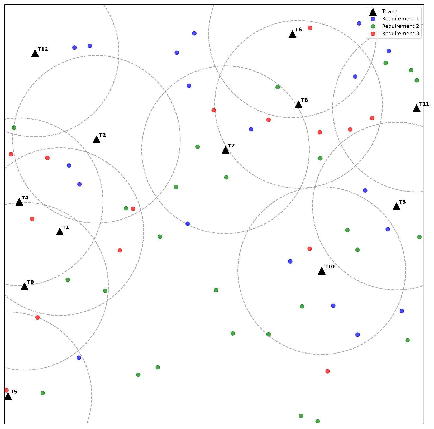
Figure 1. Illustration of covering problems with generalized coverage requirements.
Symmetry 17 01417 g001
Figure 2. Illustration of covering relationships among facilities and demand points.
Symmetry 17 01417 g002
Figure 3. Illustration of H j . The purple balls represent the set of six facilities that can serve a demand point j ( | I ( j ) | = 6 ), which requires coverage from at least three of them ( M j = 3 ). The set H j consists of all subsets H k I ( j ) with cardinality | H k | = | I ( j ) | M j + 1 = 4 , that is, the collection of subsets represented by the green balls in the figure, namely H 1 , , H 15 .
Symmetry 17 01417 g003
Figure 4. Performance profile of G-MCLP with | J | = 30,000 (left); 50,000 (middle); and 70,000 (right).
Symmetry 17 01417 g004
Figure 5. Performance profile of G-PSCLP with | J | = 30,000 (left); 50,000 (middle); and 70,000 (right).
Symmetry 17 01417 g005
Figure 6. Population distribution map of London.
Symmetry 17 01417 g006
Table 1. Parameter settings for instance generation.
ParameterSymbolValues
Number of demand points | J | {30,000, 50,000, 70,000}
Coverage radiusR{3.5, 4, 4.5}
G-MCLP:
BudgetB{10, 15, 20}
G-PSCLP:
Covering demandD{50% D ¯ , 60% D ¯ , 70% D ¯ }
Table 2. Performance comparison of BEN and CPX on G-MCLP instances.
| J | B#BENCPX
#  opt t (s) #  opt t (s)
30,00010303010.7927172.04
15303099.6120474.39
203025302.5421602.77
50,00010303017.9125321.88
15303099.6517588.93
203027327.1511808.23
70,00010303022.9123534.98
153030126.1511797.32
203027335.675923.67
Table 3. Performance comparison of BEN and CPX on G-PSCLP instances.
| J | D#BENCPX
#  opt t (s) #  opt t (s)
30,00050% D ¯ 303012.213094.88
60% D ¯ 303052.6030168.03
70% D ¯ 3030151.1730274.32
50,00050% D ¯ 303024.8230248.57
60% D ¯ 302993.5027484.62
70% D ¯ 3029318.4622655.07
70,00050% D ¯ 303025.1429478.35
60% D ¯ 3028136.0018785.11
70% D ¯ 3024490.638914.20
Table 4. Performance comparison of BEN and CPX on ultra-large G-MCLP instances.
| J | B#BENCPX
#  opt t (s) #  opt t (s)
100,0002303016.00231573.58
43030202.96112894.60
630281256.3583109.51
150,0002303035.20122937.76
43030417.0563456.12
630221840.5013569.20
200,0002303049.1293280.43
43030624.4003600.00
630202359.0103600.00
Table 5. Performance comparison of BEN and CPX on ultra-large G-PSCLP instances.
| J | DBENCPX
# opt t (s) # opt t (s)
100,00010% D ¯ 309.0530206.62
30% D ¯ 22977.03221280.16
50% D ¯ 161930.91162713.50
150,00010% D ¯ 3019.5129433.24
30% D ¯ 211146.02211904.84
50% D ¯ 102745.0293260.81
200,00010% D ¯ 3027.4728725.26
30% D ¯ 201224.67182564.32
50% D ¯ 72927.8803600.00
Table 6. Performance comparison of BEN and TABU on G-MCLP instances.
| J | B#BENTABU
10,0001030278,624.63282,947.70
1530376,182.40328,145.03
2030436,640.17340,717.60
15,0001030416,225.57400,157.03
1530560,630.20455,275.20
2030654,453.27474,509.17
20,0001030552,271.83504,916.73
1530747,655.07561,071.20
2030871,002.17578,468.43
Table 7. Performance comparison of BEN and TABU on G-PSCLP instances.
| J | D#BENTABU
10,00050% D ¯ 3029.5732.80
60% D ¯ 3036.9741.00
70% D ¯ 3045.0349.93
15,00050% D ¯ 3029.3332.87
60% D ¯ 3036.4340.77
70% D ¯ 3044.9050.10
20,00050% D ¯ 3029.7332.80
60% D ¯ 3036.9740.67
70% D ¯ 3045.6750.20
Table 8. Performance comparison of BEN and CPX on real-world G-MCLP instances.
| I | B#BENCPX
# opt t (s) # opt t (s)
80230303.19241658.09
4303018.9243380.11
63030159.5933388.45
100230306.52152574.98
4303064.4323461.90
63026968.0603600.00
1202303014.53142591.83
43030377.5103600.00
630142444.7503600.00
Table 9. Performance comparison of BEN and CPX on real-world G-PSCLP instances.
| I | DBENCPX
# opt t (s) # opt t (s)
8010% D ¯ 309.4130163.33
30% D ¯ 29456.13281257.67
50% D ¯ 23426.3123391.14
10010% D ¯ 3016.5830311.83
30% D ¯ 26959.03221922.39
50% D ¯ 03600.0003600.00
12010% D ¯ 3026.1130146.35
30% D ¯ 241153.82211929.45
50% D ¯ 03600.0003600.00
Disclaimer/Publisher’s Note: The statements, opinions and data contained in all publications are solely those of the individual author(s) and contributor(s) and not of MDPI and/or the editor(s). MDPI and/or the editor(s) disclaim responsibility for any injury to people or property resulting from any ideas, methods, instructions or products referred to in the content.