Abstract
Complex engineering systems—such as ultra-long horizontal wells in energy exploitation and distributed rail transit infrastructure—operate under harsh physical and environmental conditions, where accurate physical modeling and real-time parameter estimation are essential for ensuring safety, efficiency, and reliability. Traditional empirical and black-box data-driven approaches often fail to account for the underlying physical mechanisms, thereby limiting interpretability and generalizability. To address this, we propose a unified framework that integrates physics-informed scenario-based modeling with data-driven parameter inversion. In the first stage, critical system parameters—such as friction coefficients in drill string movement or contact forces in rail–wheel interactions—are explicitly formulated based on mechanical theory, leveraging symmetries and boundary conditions to improve model structure and reduce computational complexity. In the second stage, model parameters are identified or updated through inverse modeling using historical or real-time field data, enhancing predictive performance and engineering insight. The proposed methodology is demonstrated through two representative cases. The first involves friction estimation during tripping operations in the SU77-XX-32H5 ultra-long horizontal well of the Sulige Gas Field, where a mechanical load model is constructed and field-calibrated. The second applies the framework to rail transit systems, where wheel–rail friction is estimated from dynamic response signals to support condition monitoring and wear prediction. The results from both scenarios confirm that incorporating physical symmetry and data-driven inversion significantly enhances the accuracy, robustness, and interpretability of engineering analyses across domains.
1. Introduction
Engineering systems deployed in energy exploration and rail transit infrastructures are often subject to harsh and dynamic environments, requiring accurate physical modeling and real-time parameter estimation to ensure operational safety, reliability, and performance [1,2]. For instance, in ultra-long horizontal drilling, the interaction between drill pipe and casing leads to complex frictional behaviors that significantly influence load transfer and sticking risk [3]. In rail transportation systems, wheel–rail contact conditions—particularly friction coefficients—critically affect wear, energy consumption, and safety [4].
Traditional methods for parameter estimation are predominantly empirical or rely on black-box machine learning models. While data-driven approaches can achieve high performance when ample labeled data are available, they often lack physical interpretability and generalization across scenarios [5]. Recent advances in modeling lightweight periodic sandwich structures, such as lattice sandwich shells with truss cores, have demonstrated significant improvements in vibroacoustic performance and sound transmission loss characteristics [6]. Such innovative modeling approaches can provide valuable insights for the development of complex structural models in engineering applications. Conversely, purely physics-based models, though interpretable, are sensitive to parameter uncertainty and may be computationally prohibitive in complex systems.
To address these challenges, we propose a unified framework that combines physics-informed modeling and data-driven inversion. The proposed method first constructs mathematical models based on mechanical or wave theories, with special attention to leveraging the symmetry and boundary conditions inherent in the physical system. These structural properties improve model expressiveness and reduce the complexity of numerical solvers. Subsequently, critical parameters—such as friction coefficients or contact stiffness—are identified through inverse modeling techniques using historical or real-time measurements [7].
We validate the proposed methodology in two engineering contexts. The first is friction estimation in the SU77-XX-32H5 ultra-long horizontal well in the Sulige Gas Field, where we establish a mechanical load transmission model and back-calculate the tripping friction coefficient from field data. The second application focuses on rail transit, where wheel–rail friction coefficients are inferred from vibration response signals to support wear analysis and preventive maintenance. These case studies demonstrate the adaptability and effectiveness of our approach in both energy and transportation domains.
The main contributions and novelty of this work are summarized as follows:
- Cross-domain applicability: We propose a unified modeling framework that integrates physics-informed modeling and data-driven parameter inversion, which can be applied to both ultra-long horizontal well operations and rail infrastructure monitoring. This generalization across domains is rarely addressed in prior works.
- Symmetry-aware physical modeling: Our framework leverages the symmetry properties of governing equations and boundary conditions, improving model interpretability, reducing computational complexity, and preserving physical consistency.
- Physics-guided inverse modeling: Instead of using a black-box data-driven approach, we formulate parameter estimation as an inverse problem grounded in mechanical theory and system dynamics, allowing more robust and explainable inference.
- Real-world validation: The framework is validated through two practical case studies in energy and transportation systems. The consistent accuracy of the results highlights its potential for deployment in field applications.
The remainder of this paper is organized as follows: Section 2 reviews related work; Section 3 introduces the physical modeling approach; Section 4 presents the data-driven estimation method; Section 5 discusses the casing running case study; Section 6 explores the railway friction estimation case study; and Section 7 concludes the paper.
2. Related Work
Integrating physical knowledge with data-driven modeling has become a central research trend in scientific machine learning, particularly for improving the interpretability, generalizability, and robustness of predictions in engineering systems [5,7,8,9]. Physics-informed neural networks (PINNs) offer a compelling framework by embedding differential equations as soft constraints [10,11], but their effectiveness often declines in real-world industrial scenarios due to noise, complexity, and ill-posed boundary conditions [12]. The reviewed work highlights the importance of integrating multi-scale mathematical modeling and simulation to tackle complex physical and chemical processes in subsurface energy storage [13]. Such comprehensive approaches, considering phase equilibrium and material interactions, inspire the development of hybrid physics-informed and data-driven frameworks for engineering applications like casing running and rail infrastructure monitoring.
In the petroleum industry, the modeling of casing running forces and drag torque in horizontal wells has long been addressed via mechanical or semi-empirical models [14,15,16]. These approaches incorporate frictional contact, torque–drag analysis, and wellbore curvature, but they lack adaptability in variable formations and rarely integrate data-driven feedback. Commercial simulators (e.g., Landmark, Drillbench) are widely used, yet they often require expert calibration and are not automatically adaptive to real-time conditions [17,18].
Data-driven inversion techniques have seen significant applications in structural health monitoring (SHM), especially using distributed acoustic sensing (DAS) [19,20,21]. By treating optical fiber as a dense sensor array, DAS enables spatially continuous monitoring, with signal processing and machine learning models assisting in mode decomposition, anomaly detection, and physical interpretation [22,23,24].
Recent research also explores symmetry-aware modeling and physics-based regularization to stabilize inversion in wave propagation problems [25,26,27]. Graph-based and attention-based neural networks further improve the fusion of physics priors with sequential sensor data, especially under partial observability [28,29].
Despite these advances, many industrial drilling operations still rely on empirical rules for casing running decisions, such as selecting floating or rotating casing techniques, without sufficient theoretical support or model-driven evaluation. This leads to inefficient planning and increased risk in ultra-long horizontal well sections. To address this, our work integrates physical simulations with data-driven regression models for systematic friction coefficient estimation and casing running feasibility analysis [30,31].
Unlike traditional physics-only or black-box data-driven methods, our framework leverages the structure-preserving characteristics of physics-based modeling and the flexibility of data inversion. We demonstrate its applicability in both ultra-deep well casing operations and rail transit friction estimation, providing a unified approach for cross-domain engineering scenarios.
3. Model
3.1. Scenario-Based Physical Modeling and Assumptions
In the context of casing running in ultra-long horizontal wells, the primary resistance encountered during tripping operations is the axial friction force generated along the wellbore. To evaluate the safety and feasibility of casing operations, a physical model is established to estimate the friction coefficient based on mechanical load equilibrium.
To enable tractable modeling and parameter inversion across the engineering scenarios studied, we introduce the following key assumptions:
- Symmetry of structural and operational conditions: We assume that the underlying structures (e.g., wellbore geometry or the rail–wheel interface) exhibit symmetry in either geometry or loading, which allows for simplification in the formulation of boundary conditions and accelerates convergence during parameter inversion.
- Quasi-static or slowly varying dynamics: The system dynamics are assumed to be quasi-static or slowly varying, such that transient effects like inertia or short-term oscillations are either negligible or can be averaged out. This assumption supports the use of steady-state models for identifying parameters such as friction forces.
- Decoupled parameter influence: We assume that the primary variables influencing friction (e.g., velocity, normal load, and motor torque) have a dominant and approximately decoupled effect. This facilitates stable inverse modeling without the need for highly nonlinear multi-parameter interactions.
- Stationarity within each operating scenario: Within each defined operating case (e.g., dry, rainy, or snowy conditions), the statistical characteristics of the friction behavior are assumed to remain stable over the observation window. This permits the use of single-condition calibration for each environmental scenario.
These assumptions reflect common simplifications adopted in physics-guided modeling and are necessary to ensure generalizability and robustness of the proposed framework across domains.
3.1.1. Axial Force Equilibrium Model
Assuming a quasi-static process during casing running, the axial force distribution along the casing string can be described by a differential force balance equation. Let the key variables be defined as follows:
- : Axial tension (N) at depth z;
- : Vertical component of casing weight per unit length (N/m);
- : Friction force per unit length (N/m);
- : Dynamic friction coefficient (dimensionless);
- : Inclination angle of the well at depth z (rad);
- : Normal contact force per unit length (N/m).
The equilibrium equation for the casing segment at depth z is given by
Assuming the casing contacts the borehole wall uniformly, the normal force can be approximated as
Integrating Equation (3) from the casing shoe depth to the wellhead , the total hook load can be computed as
3.1.2. Estimation of Friction Coefficient
Given field measurements of hook load during casing running, as well as a known well trajectory and casing weight profile , Equation (4) can be inverted numerically to estimate the effective friction coefficient .
In practice, is typically constant for a uniform casing string, and is obtained from the well trajectory survey. The friction coefficient is then optimized by minimizing the error between measured and simulated hook loads:
This estimated serves as the effective tripping friction coefficient for this well, and it can be used to validate or calibrate forward simulation models and to compare different casing running strategies.
3.1.3. Symmetry and Boundary Conditions
Exploiting the inherent symmetry of engineering systems is essential to simplify physical models and reduce computational complexity without sacrificing accuracy. In the context of casing running in a horizontal wellbore, the well trajectory often exhibits axial symmetry in certain segments, particularly in straight build-up or hold sections. This allows for simplification of 3D models to effectively 1D or 2D axial profiles, assuming radial symmetry in casing–borehole contact forces.
Let us denote the axial symmetry axis along the measured depth z and assume that lateral deviations are small and distributed uniformly. Under this assumption, the friction force and normal force distributions can be expressed as functions of z only, significantly reducing model dimensionality.
In structural monitoring based on motor-side measurements, symmetry assumptions remain crucial. For example, the mechanical components within the motor and drivetrain often exhibit geometric and boundary condition symmetries. Incorporating these symmetries into the modeling of vibration and friction dynamics enhances model interpretability and ensures accurate representation of energy transfer and conservation.
- Fixed-end boundary: or (zero displacement);
- Free-end boundary: (zero stress);
- Symmetric domain: for symmetric structures.
Proper treatment of boundary conditions is critical when solving inverse problems, as they directly influence the well-posedness and uniqueness of parameter estimation.
3.1.4. Governing Equations for Mechanical and Acoustic Systems
The governing equations for the two physical systems considered in this study—mechanical casing running and structural acoustic wave propagation—are both derived from fundamental conservation laws.
- 1.
- Mechanical System: Casing Tension Model
The quasi-static axial load in the casing string is governed by a first-order differential equation derived from force balance, as previously established:
Here, is the axial tension, is the friction coefficient, is the weight per unit length, and is the inclination angle. This ODE is subject to boundary conditions at the casing shoe and surface.
- 2.
- Acoustic System: 1D Wave Propagation Model
In the structural health monitoring of rails, longitudinal acoustic wave propagation can be modeled by the 1D wave equation:
where the following applies:
- is the displacement at position x and time t;
- c is the wave speed in the medium, determined by material stiffness and density.
To model micro-crack or damage effects, a spatially varying stiffness term can be introduced, modifying the wave equation as
Here, reflects local stiffness reductions due to structural defects, and is material density. This formulation enables the inversion of from observed wavefield perturbations, providing a mechanism for damage localization.
- 3.
- Coupled Interpretation
Though mechanically distinct, both models rely on similar structures: a differential governing equation constrained by physical parameters and boundary conditions. This structural similarity allows the proposed modeling and inversion framework to be extended from downhole operations to rail-based monitoring.
3.2. Data-Driven Parameter Inversion
While physics-based models provide a structured understanding of system behavior, many critical parameters (e.g., friction coefficient in drilling or local stiffness in rail structures) are not directly measurable. Therefore, we formulate the estimation of these parameters as inverse problems, leveraging observed data to infer hidden physical quantities. This section outlines the inverse problem formulation, calibration methodology, and robustness analysis of the proposed framework.
3.2.1. Inverse Problem Formulation
Let denote a forward model governed by physical laws, where is the vector of unknown parameters (e.g., in mechanical models and in wave models), and let be the observed data (e.g., hook load or acoustic waveforms).
The inverse problem seeks to estimate such that the model output matches the observations as closely as possible:
where is a loss function, typically the mean squared error (MSE) or relative error.
For the casing running application, this becomes
For rail structure monitoring, where varies spatially, a regularized inversion problem is solved:
where is a regularization coefficient that penalizes non-smoothness in the estimated stiffness profile.
3.2.2. Calibration with Historical and Real-Time Data
Model calibration is performed by solving the inverse problems defined above using either historical operational logs or real-time sensor data:
- Historical data: For example, hook load vs. depth profiles recorded during previous casing runs, used to back-calculate average friction coefficients;
- Real-time data: For example, acoustic strain or vibration measurements collected from fiber-optic sensors during train passage, used to infer stiffness anomalies in rail tracks.
The optimization problem (Equation (9)) is solved using gradient-based or derivative-free methods depending on model smoothness and differentiability. For low-dimensional parameters like , a grid search or golden-section search may suffice. For high-dimensional parameters like , adjoint-based gradient descent or Bayesian inference methods may be applied.
Model predictions are then compared to the validation set or to field outcomes for verification.
3.2.3. Sensitivity Analysis and Model Robustness
To ensure the reliability of the inversion results, sensitivity analysis is conducted to quantify the impact of input uncertainty on the estimated parameters. For a scalar parameter such as , the sensitivity can be approximated as
For distributed parameters like , sensitivity maps are computed using the Fréchet derivative of the model output with respect to :
These maps indicate spatial regions where the model output is most sensitive to structural damage, providing insight into sensor placement and noise robustness.
Monte Carlo simulations and bootstrapping are also used to test the stability of inversion under noisy or incomplete data. A robust model will produce consistent estimates with small variance across perturbed inputs.
4. Data-Driven Parameter Identification Framework
4.1. Training Stage
The proposed framework for parameter identification in complex engineering systems consists of five major stages: synthetic data generation, real-world data acquisition, data preprocessing, pretraining with synthetic data, and model refinement using transfer learning, as illustrated in Algorithm 1.
- 1.
- Synthetic data generation: A physics-informed simulation model is constructed to generate large-scale synthetic datasets that capture the essential system behaviors under varying conditions. To optimize training efficiency, the simulation abstracts away non-essential details such as switching noise or high-frequency disturbances, while retaining key patterns related to the target parameters. For example, in a mechanical system, the simulator may numerically solve altered dynamic equations under different parameter settings (e.g., friction coefficients and damping ratios) and output the corresponding system trajectories.
- 2.
- Experimental data acquisition: Field data are collected from sensors installed in the target system (e.g., vibration signals, motor currents, and structural responses). These real-world measurements are used to fine-tune the pretrained model, allowing it to adapt to system-specific characteristics such as hardware-induced disturbances, manufacturing tolerances, and environmental noise. Full coverage of the entire parameter space is not required, as the pretrained model already encodes generalized representations.
- 3.
- Data preprocessing: To enable continuous monitoring and robust inference, raw sensor data are collected in sliding windows of fixed length at a given sampling frequency. Each windowed sample is then transformed into a suitable format for neural network input—e.g., spectral features via FFT or time-domain sequences normalized and reshaped as multichannel inputs.
- 4.
- Pretraining with synthetic data: The synthetic dataset is used to pretrain a deep neural network that learns to associate input signal patterns with corresponding engineering parameters. For instance, a convolutional architecture may be trained to classify or regress system states across a range of simulated parameter settings. This stage enables the model to generalize across diverse system configurations and operating regimes.
- 5.
- Transfer learning with experimental data: While the synthetic and experimental data share dominant structural features, transfer learning is employed to adapt the pretrained model to subtle real-world variations. Fine-tuning with experimental data allows the model to account for noise, sensor imperfections, and boundary effects, thereby improving the accuracy and reliability of parameter identification in deployment environments.
| Algorithm 1: Online Parameter Estimation via Physics-Informed Neural Inference |
 |
4.2. Uncertainty Quantification Strategy
In practical engineering scenarios, various sources of uncertainty may affect sensor readings, environmental conditions, or system parameters. To address this, we adopt a statistical strategy for uncertainty quantification when such factors are present. Specifically, two complementary techniques are employed: Monte Carlo simulation and bootstrapping.
Monte Carlo simulation is used to explore how small variations in system inputs—such as noisy sensor data or fluctuating operational loads—can influence the final estimation results. By repeatedly sampling from plausible input ranges and re-running the estimation process, we are able to characterize the distribution and stability of the predicted parameters.
In parallel, a bootstrapping approach is applied to estimate the confidence bounds of the model parameters. This involves generating multiple subsets of the available data through resampling, each of which is independently used for parameter calibration. The resulting variability across these calibrations provides empirical insight into the reliability of the parameter estimates.
These methods are only invoked when the system exhibits notable uncertainties—such as seasonal environmental variation in rail monitoring or dynamic downhole disturbances in drilling operations. In such cases, the combination of Monte Carlo simulation and bootstrapping enhances the credibility and robustness of the data-driven modeling process.
4.3. Coupling of Physical Modeling and Data-Driven Learning
In our proposed framework, physical modeling and data-driven methods are integrated in a decoupled yet complementary manner. Unlike traditional physics-informed neural networks (PINNs), where physical constraints are embedded directly into the loss function through partial differential equations, our approach leverages physical knowledge primarily during the preprocessing and post-processing stages.
During the preprocessing phase, physical models are employed to generate physically plausible input features and to filter out data inconsistencies. This includes the use of boundary conditions, symmetry properties, and domain-specific governing equations to narrow the feasible solution space. For instance, under known boundary constraints, we derive parametric relations that guide the initialization of the learning model.
In the post-processing phase, the outputs of the data-driven model are validated and corrected using physical consistency checks. These include conservation laws, threshold constraints, and system-specific behavioral expectations. If necessary, results are adjusted through lightweight regularization procedures or re-projection onto the physically valid manifold defined by the governing equations.
This modular strategy enables us to retain the flexibility and learning capacity of modern data-driven models while ensuring that outputs remain physically interpretable and compliant with known theoretical constraints. Moreover, by avoiding the direct embedding of complex equations into the training loop, our framework improves training efficiency and scalability to larger or noisier datasets.
4.4. Implementation Stage
After the final parameter identification model is developed during the training stage, the implementation stage deploys this model for continuous online monitoring and real-time parameter estimation in the target engineering system. The monitoring logic proceeds as follows:
- 1.
- Sampling: Continuously collect raw sensor signals (e.g., structural vibrations, motor currents, and pressure waveforms) at a predetermined sampling frequency and window size.
- 2.
- Feature transformation: Convert the sampled data into the same feature representation used during training. This may involve applying fast Fourier transforms (FFTs), wavelet decomposition, or normalization procedures to extract meaningful signal characteristics.
- 3.
- Model inference: Input the preprocessed feature vectors into the trained identification model to estimate the target engineering parameters (e.g., friction coefficient, local stiffness, and damping ratio).
- 4.
- Result interpretation: Analyze the output of the model to update the parameter status. The output may be a scalar value (e.g., estimated friction coefficient), a spatial distribution (e.g., stiffness profile), or a classification (e.g., normal vs. degraded state).
- 5.
- System reset: After inference, reset the temporary memory by clearing raw data buffers and retaining only the model and preprocessing configurations.
- 6.
- Repeat cycle: Restart the monitoring cycle from Step 1 for continuous operation.
4.5. Scalability and Generalizability of the Proposed Framework
Including a brief discussion on the scalability of the method to other domains or multi-physics problems further highlights the generalizability of the approach. The proposed hybrid framework integrates physics-informed modeling and data-driven inversion in a modular and extensible manner. This modularity is not only evident in its computational structure but also in its conceptual design, allowing it to be adapted to various physical systems with different governing mechanisms.
In its current implementation, the framework has demonstrated effectiveness in domains such as casing running operations in ultra-long horizontal wells and the estimation of rail–wheel contact friction. Both applications exhibit domain-specific complexities—ranging from nonlinear interactions and heterogeneous boundary conditions to limited sensor observability—and yet the framework is able to uncover hidden physical parameters and dynamic characteristics effectively. This provides an empirical basis for extending the method beyond these specific domains.
Importantly, many real-world engineering systems are governed by coupled physical processes. The scalability of the proposed method lies in its ability to encode such coupling into the hybrid model. Another crucial advantage of the framework is its capability to handle sparse, noisy, or asynchronous data, a common trait in multi-physics problems where sensor placement and measurement frequency are limited by practical considerations. By incorporating physical priors, the method can regularize the inversion problem and reduce the reliance on dense measurements, enhancing robustness and generalization.
5. Case Study I: Casing Running Construction Challenges
5.1. Background of Sulige Gas Field
The Sulige Gas Field, located in the Ordos Basin, is China’s first large-scale tight gas field. Its reservoirs are characterized by low pressure, low permeability, low productivity, and low abundance—commonly referred to as the “four lows”—which have long constrained the efficient development of tight gas resources. To address the challenges of economically developing tight gas, horizontal wells have been increasingly deployed in the field due to their advantages in accessing longer reservoir sections and achieving higher production rates.
The SU77-XX-32H5 well is located in Block SU77, situated in the northern part of the eastern Sulige Gas Field, with proven geological reserves of 74.282 billion cubic meters. A total of 59 horizontal wells have been completed in this block, with an average horizontal section length of only 1165 m. To further expand the drainage area, enhance single-well productivity, and effectively utilize reserves within environmentally protected zones, the SU77-XX-32H5 well was drilled with a horizontal section length of 3000 m—158% longer than the block average—setting a new record for the longest horizontal section in the area. However, with increasing horizontal section length, significant technical challenges arise in efficiently running the production casing.
5.2. Geological Challenges
The Ordos Basin features an asymmetrical synclinal structure, characterized by uplifted regions in the north and south, a gently sloping and extended eastern flank, and a short, steep western flank. Based on these structural characteristics, the basin is divided into six major secondary tectonic units. The SU77-XX-32H5 well is located in the northern part of the Shaanbei Slope within the Ordos Basin. During drilling, the encountered strata from top to bottom include the Quaternary, the Cretaceous Luohe Formation, the Jurassic Anding, Zhiluo, and Yan’an Formations, as well as the Triassic Yanchang, Zhifang, Heshanggou, and Liujiagou Formations, and the Permian Shiqianfeng and Shihezi Formations.
The target formation is the Shihezi Formation, which features well-developed and laterally extensive sand bodies. The lithology is primarily composed of gray, grayish-white, and greenish-gray conglomeratic sandstones interbedded with brown-gray and dark-gray argillaceous sandstones. The formation is characterized by high collapse pressure and poor wellbore stability. During casing running operations in ultra-long horizontal sections, the wellbore is highly prone to instability, leading to borehole collapse and the accumulation of debris, which can easily cause casing sticking and obstruction.
5.3. Engineering Challenges
As shown in Figure 1, the horizontal wells in the tight gas reservoir of Block SU77 mainly adopt a three-section wellbore structure. The first section is drilled with a bit to a depth of , followed by running a surface casing to seal the upper loose formations. The second section uses a bit to reach the kickoff point of the horizontal well, where a technical casing is run to facilitate targeted drilling of the reservoir. The third section, the horizontal interval, is drilled with a bit to the final target, and a production casing is run to complete the well. The casing running operation during completion faces the following four key engineering challenges:
- 1.
- High horizontal-to-vertical ratio. The SU77-XX-32H5 well has a horizontal section of and a maximum true vertical depth of , resulting in a horizontal-to-vertical ratio of . During casing running—especially along the extended horizontal section—the self-weight of the casing provides insufficient driving force. Meanwhile, the contact area between the casing and the wellbore gradually increases, leading to higher friction, which hinders efficient casing deployment.
- 2.
- Complex well trajectory. To meet geological requirements, the well is designed with a seven-section 3D trajectory: vertical–build–hold–build with torque increase–build–slight build–horizontal. The horizontal displacement before the target is , and the build section is long. In practice, frequent vertical trajectory adjustments were made to maximize reservoir contact. These adjustments lead to multiple contact points between the casing and the borehole during running, causing significant lateral forces and frictional resistance, which impede casing efficiency.
- 3.
- Difficulties in borehole cleaning. The long horizontal section results in high annular pressure losses and limited circulation rates. Cuttings are transported slowly in the horizontal interval, easily forming extended cutting beds, which obstruct casing running.

Figure 1.
Horizontal wells.
In our axial force equilibrium model, we assume uniform contact between the casing and the borehole wall to estimate the distributed normal force along the well trajectory. However, in practical horizontal and extended-reach wells, especially in sections with high dogleg severity (DLS) or frequent trajectory adjustments, this assumption may not hold. The actual contact is often intermittent and localized, resulting in a non-uniform distribution of contact forces.
Such deviations may lead to overestimation or underestimation of the normal force and friction resistance, particularly in complex trajectories where wellbore irregularities (e.g., borehole enlargement or spiraling) are significant. To address this limitation, future work could introduce a correction factor to adjust the normal force profile based on local geometrical properties of the wellbore. For instance, DLS can be used as a proxy for contact severity, and borehole caliper data may offer further refinement of contact models.
While the current study focuses on a generalized analytical framework without incorporating such corrections, we acknowledge this as an important direction for enhancing model realism and generalizability. A brief discussion on this point has been added to emphasize the potential improvement.
5.4. Maximum Passable Curvature Evaluation
When the borehole curvature in a bent section is relatively large, the casing may experience excessive bending stress while passing through, potentially leading to deformation or failure. Based on the maximum axial stress under pure bending and the relationship between borehole curvature and casing curvature, the axial stress under pure bending can be expressed as
where the following applies: is the axial stress in the casing (MPa); E is the elastic modulus of the casing material (Pa); is the outer diameter of the casing (m); C is the borehole curvature (rad/m); L is half the distance between two casing couplings (m); T is the tensile force on the lower casing in the curved section (N); I is the moment of inertia of the cross-section ().
When the axial stress reaches the casing yield strength, the critical borehole curvature can be obtained from the strength condition as
where is the yield strength of the casing body (Pa).
In engineering practice, borehole curvature is commonly expressed as the dogleg severity per 30 m. By unifying the units and incorporating the thread stress concentration factor and the bending safety factor, Equation (2) can be rewritten as
When the tensile force on the lower casing in the curved section is small, , Equation (3) simplifies to
where the following applies: is the maximum allowable borehole curvature for casing passage (°/30m); is the bending safety factor (typically 1.8 for API and 2.0–2.5 for IADC); is the thread stress concentration factor (typically 3.0 for API and 2.0–2.5 for IADC).
Equation (4) is the recommended formula for the maximum allowable borehole curvature for casing running according to API and IADC standards.
Based on the above formulas and assuming the most conservative case (maximum safety factors), the calculated maximum allowable borehole curvature for casing running in the SU77-XX-32H5 well is /. According to the actual well trajectory data, the maximum continuous three-point dogleg severities are , , and per 30 m, all of which are below the critical curvature, indicating that casing running is theoretically feasible.
5.5. Selection of Casing Running Method
5.5.1. Experimental Platform and Computational Environment
To validate the real-time applicability and computational efficiency of the proposed method, all experiments were conducted on an edge computing device—the NVIDIA Jetson Orin Nano 8 GB. This platform features a 6-core ARM Cortex-A78AE CPU, a 1024-core NVIDIA Ampere GPU architecture, and 32 third-generation Tensor Cores, delivering up to 40 TOPS (Tera Operations Per Second) of AI performance under a configurable power envelope of 7–15 W. Such a hardware setup is well-suited for embedded scenarios with strict constraints on power consumption and space, such as intelligent vehicles and autonomous sensing systems. The lightweight design and efficient architecture allow for real-time processing directly on-device, without relying on external servers or cloud infrastructure.
In the implementation of our data-driven parameter identification framework, we employed a feedforward neural network consisting of four fully connected layers with 128, 64, 32, and 16 neurons, respectively. Each layer uses the ReLU activation function except for the output layer, which uses a linear activation to regress the target parameters. The model was trained using the Adam optimizer with an initial learning rate of and a batch size of 64. Early stopping was applied with a patience of 10 epochs to prevent overfitting. The synthetic dataset used for pretraining was generated based on the physical model with parameter variations sampled uniformly within realistic engineering bounds, ensuring coverage of the plausible operating space. To bridge the domain gap between synthetic and real data, transfer learning was performed by fine-tuning the pretrained model using a small real-world dataset collected from field measurements. To mitigate distribution shifts, we applied normalization strategies based on the statistics of the real data and visually verified the alignment between synthetic and real data distributions using kernel density estimates and principal component projections.
The Sulige Gas Field case study was conducted based on historical production data and archived well logs, rather than real-time field measurements. Specifically, parameters such as friction factors, hook loads, and borehole trajectories were estimated through the integration of legacy drilling reports, logging interpretations, and engineering heuristics. These data were processed and calibrated under the guidance of experienced field engineers to ensure the representativeness of the simulated operating conditions. While this approach offers valuable insight into the applicability of the proposed model, it inherently carries uncertainties due to possible discrepancies between historical estimates and real-time dynamics. Therefore, the simulation results should be interpreted as a scenario-based evaluation rather than a precise replication of live operational data.
5.5.2. Back-Calculation of Drilling Friction Factor
The friction coefficient obtained through measurements can only relatively reflect the smoothness of the borehole mud cake and cannot comprehensively represent the overall borehole friction condition. The friction factor (FF) differs from the friction coefficient; it is an attribute parameter that includes all influencing factors of friction. These influencing factors cannot be measured directly, such as cuttings beds, borehole ledges, spirality, tool centralization, and tool weight errors. The friction factor can comprehensively reflect the magnitude of borehole friction.
By calculating the mechanical load of the drilling assembly during open-hole drilling, a suspended weight sensitivity model chart for the friction factor is established. Based on actual well depth and hook load data recorded during drilling, the friction factor for open-hole drilling can be back-calculated using this chart. This provides a preliminary evaluation of the open-hole friction condition, laying the foundation for selecting borehole cleaning techniques and casing running methods, as well as accurately predicting the casing running friction factor.
As shown in Figure 2, the actual drill-in hook load data from the three-stabilizer drilling assembly in well SU77-XX-32H5 were meticulously recorded and analyzed. By employing the suspended weight sensitivity model chart, we were able to back-calculate the friction factor inside the casing, yielding a value of 0.2. This relatively low friction coefficient indicates effective lubrication and smooth casing movement during the running process. Furthermore, the open-hole drilling friction factor, denoted as , was determined to be 0.46. The higher value of reflects increased resistance encountered in the open-hole section, likely due to more complex interactions between the drill string, formation, and borehole conditions.
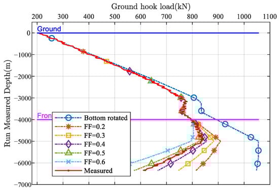
Figure 2.
Drill-in hook load data.
The consistency between these values and the operational data validates the robustness of the suspended weight sensitivity approach for friction estimation. Moreover, these friction factors serve as critical inputs for subsequent mechanical load simulations and optimization of casing running strategies. The ability to accurately quantify friction coefficients under real field conditions is essential for predicting potential sticking risks and selecting appropriate drilling parameters, especially in ultra-long horizontal well sections where frictional challenges are exacerbated.
5.5.3. Selection of Casing Running Method
Due to the high difficulty of running casing in ultra-long horizontal section wells, it is necessary to perform an adaptability evaluation of special casing running methods and compare them with conventional methods to determine the onsite casing running approach. Currently, the main special casing running techniques for horizontal wells include rotary casing running and floating casing running. Rotary casing running presents significant challenges due to the difficulty of rotation and risks of casing torsional damage, making it a high-risk option for ultra-long horizontal wells. This study focuses on comparing and selecting between floating casing running and conventional casing running methods for the casing running operation in well SU77-XX-32H5.
First, a simulation of conventional casing running for the casing in well SU77-XX-32H5 was conducted, with the results shown in Figure 3. It can be seen that when the friction factor is 0.3, the casing string exhibits localized sinusoidal buckling; when the friction factor increases to 0.4, large-scale helical buckling occurs in the section between 1660 m and 1986 m, with a remaining surface hook load of 344 kN.
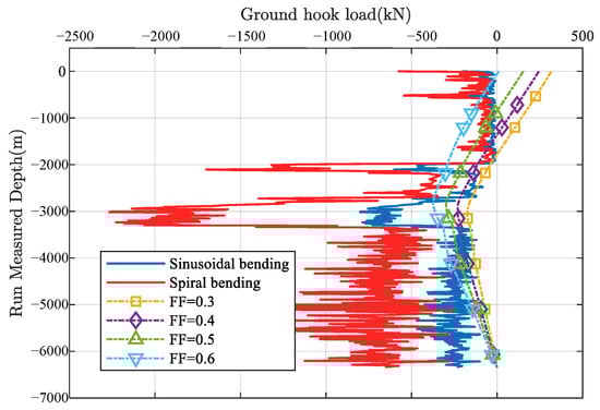
Figure 3.
Effective stress analysis of conventional casing running.
This trend can be explained by the increasing frictional resistance along the casing string, which amplifies the compressive stresses and promotes instability modes of higher amplitude and wavelength. At lower friction factors (e.g., 0.3), the frictional force is insufficient to cause extensive deformation, resulting in localized sinusoidal buckling. As the friction factor increases to 0.4, the elevated shear resistance causes the casing to experience more severe compressive loading over a longer interval, thereby inducing helical buckling that spans a larger section. The observed surface hook load increase corresponds to the additional mechanical effort required to overcome this intensified buckling, highlighting the critical influence of friction on casing stability. This interpretation aligns with fundamental mechanics principles and emphasizes the importance of accurately estimating friction factors to predict casing behavior under operational conditions.
Next, a simulation of floating casing running (with a floating section length of 3000 m) was performed for the same casing, with the results shown in Figure 4. It is observed that when the friction factor is 0.5, the casing string experiences localized sinusoidal buckling but no helical buckling; when the friction factor reaches 0.6, small-scale helical buckling occurs between 1701 m and 1966 m, with a remaining surface hook load of 347 kN.
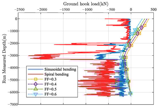
Figure 4.
Effective stress analysis of floating casing running.
Combining with the back-calculated open-hole drilling friction factor of 0.46, the analysis indicates that under current wellbore conditions, the conventional casing running method carries an extremely high risk, and the casing is unlikely to be run smoothly to the bottom. The floating casing running method theoretically reduces downhole friction by 37%, significantly improving the ability to run casing through the horizontal section. Therefore, the floating casing running technique is preferred for production casing running operations. The observed friction reduction can be attributed to the altered contact force distribution along the casing induced by the floating section. Specifically, the floating segment effectively reduces the axial contact stress between the casing and borehole wall by allowing partial mechanical decoupling, which mitigates frictional resistance during the running process. This reduction in contact stress also decreases the likelihood of casing buckling and enhances load transfer efficiency. Furthermore, the simulation results suggest that optimizing the length and position of the floating collar is critical to maximizing friction reduction, as it balances the mechanical support and flexibility of the casing string. These mechanistic insights provide a clearer physical basis for the improved performance of the floating casing running method observed in the analysis.
5.6. Optimization of Floating Collar Position
To fully leverage the advantages of the floating casing running method and minimize friction during casing running, the floating section length of the casing must be reasonably designed. A sensitivity analysis of the hook load with respect to the floating section length was conducted using specialized software to provide a theoretical basis for the installation position of the floating collar. The simulation results are shown in Figure 5.
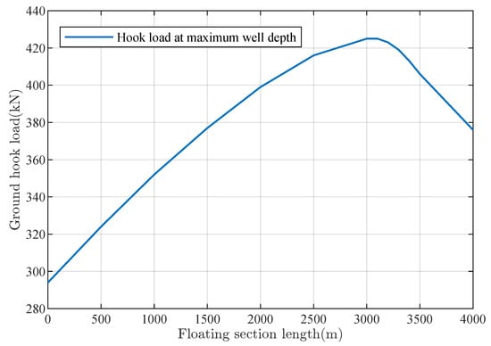
Figure 5.
Sensitivity analysis of hook load and floating section length.
As shown in Figure 5, with an increase in the floating section length, when the casing reaches the maximum well depth, the surface hook load first increases and then decreases. The hook load peaks at a floating section length of 3100 m, indicating the minimum borehole friction at this length. Based on the simulation results, the optimal floating collar placement is at 3100 m from the well bottom.
5.7. Accurate Prediction of Casing Running Friction Factor
Currently, domestic predictions of casing running friction factors often use empirical additive methods. For example, the friction factor for water-based drilling fluid casing running is estimated by adding 0.1 to the open-hole friction factor, while for oil-based drilling fluid, an addition of 0.05 is used. This method has low prediction accuracy and requires extensive similar neighboring well data in the block to correct empirical coefficients, which reduces its applicability to special wells such as ultra-long horizontal sections.
This study establishes a comparative analysis model between open-hole and casing running friction factors, as well as a model analyzing the main controlling factors of friction, to predict the casing running friction factor for well SU77-XX-32H5.
By statistically analyzing the final open-hole friction factors and actual casing running friction factors of neighboring wells in the same block, the difference in friction factors, , is calculated. The average of from multiple neighboring wells, denoted as , is used as a reference for the friction factor increment during casing running in the block.
For positive drilling, based on simulation analysis, the final open-hole friction factor is evaluated. The predicted casing running friction factor is given by
Using measured data from neighboring wells in block SU77 (Table 1), the average difference is calculated as 0.08. According to Equation (5), the predicted casing running friction factor for well SU77-XX-32H5 is

Table 1.
Measured open-hole and casing running friction factors of neighboring wells.
5.8. Analysis Model of Main Controlling Factors for Friction Factor
The friction factor analysis model compares each main controlling factor behind the casing running friction factor () of similar neighboring wells with those of the target well under rotary drilling. Using professional drilling software, the sensitivity of each main controlling factor is analyzed.
First, the “suspended weight vs. friction factor sensitivity” model of the rotary drilling casing string is normalized and compared with that of the neighboring well casing string. After calculating the neighboring well’s casing running friction factor, the corresponding suspended weight is back-calculated using the rotary drilling sensitivity model to obtain a normalized friction factor .
Next, each main controlling factor of the neighboring well is individually replaced by the corresponding factor of the rotary drilling well to calculate the positive or negative impact on the neighboring well’s casing running friction factor. These increments or decrements in friction factor are quantified to predict the casing running friction factor for the rotary drilling well. The detailed procedure is as follows:
- Selection of highly similar neighboring well. The already drilled neighboring well SU77-XX-32H3 is located on the same drilling platform as SU77-XX-32H5, with a wellhead distance of 10 m. The horizontal section length of SU77-XX-32H3 is 2569 m, which is closest to SU77-XX-32H5. Therefore, it is chosen as the reference neighboring well.
- Analysis of main controlling factors. Both wells target the same formation with similar geological conditions. The main controlling factors are concentrated on engineering aspects. By comparing actual drilling data, the main controlling factors are identified as borehole trajectory, wellbore structure, casing structure, and drilling fluid.
- Calculation of friction factor impact for each main factor. Each main controlling factor of the rotary drilling well is individually applied to the neighboring well’s casing string “suspended weight vs. friction factor sensitivity” model to calculate the increase or decrease in friction factor for casing running.
The predicted casing running friction factor for the rotary drilling well is calculated as
According to the results of the main controlling factors analysis (Table 2), the wellbore structure has the greatest impact. This is because the technical casing in SU77-XX-32H5 extends 659 m beyond the kickoff point, whereas in SU77-XX-32H3, it only extends to the kickoff point, which effectively reduces downhole friction in the rotary drilling well. The casing structure has the least impact due to both wells using floating casing running technology with similar floating section lengths. Based on Equation (6), the predicted casing running friction factor for SU77-XX-32H5 is
Table 2.
Calculation results of main controlling factors for friction factor.
5.9. Casing Running Simulation Analysis
Based on the predicted casing running friction factors described above, a simulation analysis of casing running was conducted. The basic simulation parameters are as follows:
- 1.
- Wellbore structure: Drill bit × surface casing × 501 m + drill bit × intermediate casing × 4009.36 m + drill bit × open-hole section × 6350 m;
- 2.
- Production casing data: Outer diameter , wall thickness 8.56 mm, steel grade P110, linear weight 224.7 N/m, top depth 0 m, and bottom depth 6350 m;
- 3.
- Trajectory data: Measured by MWD inclinometer, kickoff point depth 2000 m, point A depth 3350 m, inclination angle 89.58°, azimuth 1.56°, point B depth 6350 m, inclination angle 90.00°, and azimuth 359.92°;
- 4.
- Drilling fluid properties: Density 1.24 g/cm3, Bingham plastic rheology, plastic viscosity 25 mPa·s, and yield point 8 Pa;
- 5.
- Friction factors: Inside casing 0.2, and 0.54/0.56 in open-hole section;
- 6.
- Casing running method: Floating casing running with a floating section length of 3100 m.
The simulation results of casing running are shown in Figure 6. According to the prediction based on the comparative analysis model of the open-hole and casing running friction factors, when the production casing reaches the well bottom, the surface remaining hook load is 383.5 kN, and the downhole friction is 285.8 kN. According to the prediction based on the main controlling factors analysis model, the surface remaining hook load is 372.2 kN, and the downhole friction is 297.1 kN when the casing reaches the bottom. The analysis indicates that under current wellbore conditions, using the floating casing running technique, the production casing can theoretically be run smoothly to the final drilling depth.
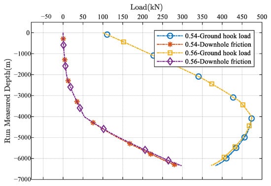
Figure 6.
Simulation results of casing running.
The slight differences between the two models in predicted hook load and friction values highlight the improved precision of the main controlling factors analysis model, which incorporates detailed geological and operational parameters. The reduced surface hook load predicted by this model suggests a more realistic estimation of frictional forces, accounting for local variations along the wellbore. Additionally, the increase in downhole friction reflects the complexity of interactions at depth, emphasizing the need for nuanced modeling to capture these effects accurately. These results collectively affirm that the floating casing running method is effective in mitigating excessive frictional resistance, thus reducing the risk of casing sticking or buckling during deployment. This detailed interpretation enhances confidence in the model’s predictive capability and supports informed decision-making for well completion in ultra-long horizontal sections.
5.10. Field Construction Situation
Well SU77-XX-32H5 commenced floating casing running operations at 2:00 AM on October 23. According to the completion string structure, the actual floating section length was fine-tuned to 3117.38 m. The casing reached the well bottom at 10:30 AM on October 24, and the floating collar opened smoothly (opening pressure 18 MPa). No incidents occurred during the operation. The total construction time was 32.5 h, which is 22% shorter compared to neighboring wells on the same drilling platform.
Based on the actual hook load data during casing running, the friction factor was back-calculated, as shown in Figure 7. It can be observed that the friction factor in the upper open-hole section was about 0.4, gradually increasing with well depth, finally reaching 0.57.
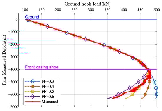
Figure 7.
Actual casing running friction factor.
6. Case Study II: Structural Monitoring in Rail Transit Infrastructure
In rail transit systems, real-time estimation of wheel–rail friction forces is crucial for ensuring operational safety, enhancing traction control, and optimizing maintenance scheduling. This section presents a case study where motor-side measurements—such as torque, current, and rotational speed—are utilized to infer track friction characteristics. By combining physical models of traction dynamics with data-driven correction techniques, the proposed method enables accurate reconstruction of frictional forces without relying on dedicated sensing infrastructure.
6.1. Friction Identification
The typical characteristics of the wheel–rail friction force are illustrated in Figure 8. In this study, the Stribeck friction model [32] is employed to characterize the nonlinear relationship between the relative velocity of the wheel–rail contact point and the resulting friction force. This model captures key behaviors such as the transition from static to kinetic friction and the velocity-weakening characteristic observed in low-speed regimes. Compared with alternative models such as LuGre or Dahl, the Stribeck model provides a good trade-off between physical accuracy and computational efficiency, especially in large-scale simulations where real-time or near-real-time performance is desired.
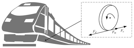
Figure 8.
Railway wheel friction force.
Although more complex models may offer improved fidelity under specific dynamic conditions, their application requires detailed knowledge of internal parameters, which are difficult to obtain or estimate in practical rail systems. Additionally, these models often introduce higher computational overhead, making them less suitable for scenarios involving large networks or long time horizons.
To simplify system analysis and enable tractable control design, we apply a piecewise linearization approach to the friction behavior in both low-speed and high-speed operating phases. This allows for the integration of friction effects into the overall system dynamics without significantly increasing model complexity. While such linearization introduces approximation errors, comparative simulations under representative operating conditions show that the deviation from full nonlinear friction models remains within acceptable engineering margins.
We acknowledge that the selection and simplification of friction models may impact overall simulation fidelity. As part of future work, we plan to conduct a comprehensive evaluation of different friction models and assess the trade-offs between accuracy and real-time applicability across various rail transit scenarios. In the proposed control framework, the reducer friction is modeled using the Stribeck formulation, which effectively captures the nonlinear behavior of friction across different velocity regimes. The mathematical expression of the Stribeck model [32] is given by
Here, is the applied external force, is the maximum static friction force, is the Coulomb friction force, B is the viscous damping coefficient, v is the relative velocity, is the Stribeck velocity, and is a shaping parameter that controls the slope of the Stribeck curve.
The input to the model is the velocity v, and the output is the friction torque. In the control system, this friction torque acts as a disturbance, which can be expressed as: .
The entire process can be divided into four distinct phases for analysis: forward low-speed, forward high-speed, reverse low-speed, and reverse high-speed phases.
In the low-speed phase, a first-order Taylor expansion can be applied to derive the linearized model for this region:
For the forward high-speed phase, a first-order Taylor expansion is performed at the peak rotational speed within the sampled data of the Stribeck model, yielding the following linearized expression:
The intersection point between the low-speed model and the mid-to-high-speed model can be computed as the intersection of two linear functions:
The same approach is applied to the reverse direction. Thus, the complete linearized Stribeck model for both forward and reverse motions can be formulated as
Hence, the identification of the Stribeck model is transformed into the fitting of four linear segments defined by corresponding parameters:
6.2. Railway Motor Model
The electrical and mechanical equations for the continuous mathematical model of a permanent magnet synchronous motor (PMSM) in the dq-axis are
where denote the d,q-axis voltages, denote the d,q-axis currents, denotes the electrical angular velocity, denotes the stator resistance, denote the d,q-axis inductances, denotes the permanent magnet flux linkage, denotes the electromagnetic torque, denotes the load torque, p denotes the number of pole pairs, J denotes the moment of inertia, and F denotes the friction coefficient.
In practical rail transit operations, track irregularities and wheel wear significantly influence the friction forces between the wheel and rail. Surface roughness, rail corrugation, and local defects can cause variations in contact pressure and friction behavior, leading to fluctuations that are not captured by idealized friction models. Similarly, wheel wear alters the contact geometry and material properties, which affects the friction characteristics over time.
Although the current friction estimation framework utilizes motor-side sensing parameters and the Stribeck friction model to capture nonlinear friction behavior, it does not explicitly account for these operational factors. Incorporating the effects of track irregularities and wheel wear is essential for enhancing model fidelity and robustness in real-world scenarios. Future work will focus on integrating sensor data related to track condition and wheel status, as well as developing adaptive friction models that dynamically adjust to these influences. This advancement will improve the accuracy and reliability of friction force estimation, thereby supporting safer and more efficient rail system maintenance and control.
6.3. Results
In this study, the frictional interaction between the downhole components and the wellbore was modeled using a Stribeck-type nonlinear friction model, and the motor dynamics were governed by a physics-based model of PMSMs. Due to the lack of access to real-time sensor data from downhole rail systems or actual motor feedback, the validation of these models was carried out using synthetic simulations. These simulations were calibrated using standard tool specifications, operational envelopes typical of horizontal drilling operations, and empirical parameter ranges reported in the prior literature. Although synthetic validation provides a controlled environment for model testing, it does not fully reflect the complexity of real-world field interactions. This limitation is acknowledged and discussed in Section 7, where future work involving real-time sensor integration is proposed to further enhance model fidelity. The proposed detection method is simulated in MATLAB-Simulink 2024b on a PMSM, the parameters of which are shown in Table 3. Typical curves are collected, as shown in Figure 9. The motor can rise up to the given value of 2000r/min smoothly, the sinusoidal degree of the three-phase current of the motor is good, and the fluctuation of the d,q-axis current is small.
Table 3.
Parameters of PMSM.
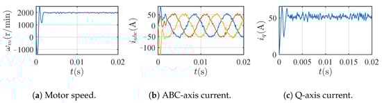
Figure 9.
Typical curves under Case 1.
Under different environmental scenarios—with Case 1 representing dry conditions in spring and autumn, Case 2 corresponding to rainy conditions in summer, and Case 3 representing snowy conditions in winter—the simulated and estimated results of rail friction forces are shown in Figure 10. The proposed estimation method demonstrates good agreement with the simulated measurements. Among the three cases, the lowest friction force is observed in Case 1, followed by Case 2, while Case 3 exhibits the highest friction force, which is consistent with real-world observations. The optimal fitting parameters identified under different operating conditions are summarized in Table 4.
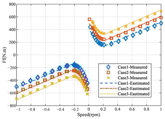
Figure 10.
Actual railway motor friction force.
Table 4.
Optimal fitting parameters under different operating conditions.
This trend reflects the influence of environmental factors on rail–wheel interface conditions. Dry scenarios (Case 1) provide minimal contamination and moisture, leading to reduced adhesion and, thus, lower friction forces. In contrast, rainy conditions (Case 2) increase surface moisture and can introduce contaminants, elevating friction moderately. Snowy conditions (Case 3) create the most challenging interface due to ice and packed snow, resulting in significantly higher friction forces. The close alignment between the estimated and simulated data across these scenarios validates the robustness of the proposed estimation framework. Moreover, the consistent seasonal variation captured by the model enhances its practical applicability for real-time rail friction monitoring and maintenance decision-making, enabling improved safety and performance in rail transit operations.
Table 5 summarizes the performance comparison among several baseline models and the proposed hybrid framework. Specifically, TPM1 refers to the physics-informed neural network approach introduced in [5], which integrates physical governing equations directly into the loss function to guide the learning process.TPM2 is based on the framework proposed in [7], leveraging partial differential equations and variational formulations to constrain neural network outputs.PDM1 corresponds to the purely data-driven deep learning model from [19], which uses temporal convolution and recurrent units to capture signal patterns without incorporating domain knowledge. PDM2 adopts a spatio-temporal graph convolutional network from [23] that models the system as a dynamic graph and learns complex relationships between sensing points over time. In contrast, the Proposed method introduces a hybrid framework that combines physical priors with data-driven representations, enabling more accurate, robust, and computationally efficient predictions by jointly exploiting physics knowledge and historical data patterns. The proposed hybrid framework achieves the highest testing accuracy (0.97) and the lowest prediction error (0.03), demonstrating superior predictive performance compared to traditional physics-based models (TPM1 and TPM2) and pure data-driven models (PDM1 and PDM2). Although the computation time of the proposed method (10.2 s) is slightly higher than TPM2, it remains significantly more efficient than the pure data-driven models, striking a favorable balance between accuracy and computational efficiency.
Table 5.
Performance comparison of different predictive models (80% training and 20% testing data).
7. Conclusions
This study presents a novel and generalizable modeling approach that combines physics-informed modeling with data-driven inversion, grounded in system symmetries and domain-specific constraints. Unlike previous works that often focus on either purely mechanistic or purely data-driven methods, our framework ensures both interpretability and adaptability across multiple engineering fields. The integration of mechanical load simulations with data-driven models enables a scientific and systematic evaluation of casing running conditions, providing a robust foundation for selecting appropriate casing running methods and optimizing completion string design in ultra-long horizontal sections. Compared with traditional comparative models based on open-hole and casing friction factors, the analysis model focusing on main controlling factors delivers more accurate and adaptable predictions—particularly in scenarios with limited offset well data, complex wellbore geometries, or special well types such as ultra-long horizontal sections. The proposed hybrid framework achieves the highest testing accuracy of 0.97 and the lowest prediction error of 0.03, outperforming traditional physics-based models (TPM1 and TPM2) and pure data-driven models (PDM1 and PDM2). Additionally, this study introduces a physics-informed estimation approach for identifying railtrack friction forces using motor-side sensing parameters. A nonlinear friction model based on the Stribeck curve effectively captures reducer behavior under varying environmental conditions. Case studies under dry (Case 1), rainy (Case 2), and snowy (Case 3) environments demonstrate that estimated friction forces closely align with simulation results, reflecting expected seasonal trends. These findings validate that motor-side signals contain sufficient information for accurate friction estimation, supporting real-world railway operational applications. Looking ahead, further improvement in the prediction accuracy of casing running friction factors will require continuous enrichment of neighboring well data sets. Supported by data analysis models, the influence of key controlling parameters can be quantified more precisely, establishing a solid data-driven basis for reliable safety evaluation of casing running in ultra-long horizontal wells. Future work will also explore the extension of this hybrid modeling framework to other complex engineering systems where both physical insights and data-driven adaptability are essential.
Author Contributions
Methodology, X.Z.; Software, X.Z.; Formal analysis, Y.C.; Writing—original draft, X.Z. and Z.T.; Writing—review and editing, Z.T. and Y.C.; Funding acquisition, Y.C. All authors have read and agreed to the published version of the manuscript.
Funding
This work was supported by the Liaoning Province Science and Technology Joint Plan (2024-BSLH-108).
Data Availability Statement
The original contributions presented in this study are included in the article. Further inquiries can be directed to the corresponding author.
Conflicts of Interest
Author Xinyu Zhang was employed by Engineering Technology Research institute of XDEC. The remaining authors declare that the research was conducted in the absence of any commercial or financial relationships that could be construed as a potential conflict of interest.
References
- Liu, W.; Tian, Z.; Xu, Y.; Zhao, M.; Li, R.; Pang, H.; Zhao, H.; Feng, Z. Drill string mechanics and extension capacity of extended-reach well. Teh. Vjesn. 2023, 30, 39–51. [Google Scholar]
- Shaikh, M.Z.; Ahmed, Z.; Chowdhry, B.S.; Baro, E.N.; Hussain, T.; Uqaili, M.A.; Mehran, S.; Kumar, D.; Shah, A.A. State-of-the-art wayside condition monitoring systems for railway wheels: A comprehensive review. IEEE Access 2023, 11, 13257–13279. [Google Scholar] [CrossRef]
- Kumar, A.; Nwachukwu, J.; Samuel, R. Analytical model to estimate the downhole casing wear using the total wellbore energy. J. Energy Resour. Technol. 2013, 135, 042901. [Google Scholar] [CrossRef]
- Fang, C.; Jaafar, S.A.; Zhou, W.; Yan, H.; Chen, J.; Meng, X. Wheel-rail contact and friction models: A review of recent advances. Proc. Inst. Mech. Eng. Part F J. Rail Rapid Transit 2023, 237, 1245–1259. [Google Scholar] [CrossRef]
- Karniadakis, G.E.; Kevrekidis, I.G.; Lu, L.; Perdikaris, P.; Wang, S.; Yang, L. Physics-informed machine learning. Nat. Rev. Phys. 2021, 3, 422–440. [Google Scholar] [CrossRef]
- Asadi Jafari, M.H.; Zarastvand, M.; Zhou, J. Doubly curved truss core composite shell system for broadband diffuse acoustic insulation. J. Vib. Control 2024, 30, 4035–4051. [Google Scholar] [CrossRef]
- Raissi, M.; Perdikaris, P.; Karniadakis, G.E. Physics-informed neural networks: A deep learning framework for solving forward and inverse problems involving nonlinear partial differential equations. J. Comput. Phys. 2019, 378, 686–707. [Google Scholar] [CrossRef]
- Cuomo, S.; Di Cola, V.S.; Giampaolo, F.; Rozza, G.; Raissi, M.; Piccialli, F. Scientific machine learning through physics–informed neural networks: Where we are and what’s next. J. Sci. Comput. 2022, 92, 88. [Google Scholar] [CrossRef]
- Brunton, S.L.; Proctor, J.L.; Kutz, J.N. Discovering governing equations from data by sparse identification of nonlinear dynamical systems. Proc. Natl. Acad. Sci. USA 2016, 113, 3932–3937. [Google Scholar] [CrossRef]
- Jin, X.; Cai, S.; Li, H.; Karniadakis, G.E. NSFnets (Navier-Stokes flow nets): Physics-informed neural networks for the incompressible Navier-Stokes equations. J. Comput. Phys. 2021, 426, 109951. [Google Scholar] [CrossRef]
- Sun, L.; Gao, H.; Pan, S.; Wang, J.X. Surrogate modeling for fluid flows based on physics-constrained deep learning without simulation data. Comput. Methods Appl. Mech. Eng. 2020, 361, 112732. [Google Scholar] [CrossRef]
- Krishnapriyan, A.; Gholami, A.; Zhe, S.; Kirby, R.; Mahoney, M.W. Characterizing possible failure modes in physics-informed neural networks. Adv. Neural Inf. Process. Syst. 2021, 34, 26548–26560. [Google Scholar]
- Feng, X.; Liu, J.; Shi, J.; Hu, P.; Zhang, T.; Sun, S. Phase equilibrium, thermodynamics, hydrogen-induced effects and the interplay mechanisms in underground hydrogen storage. Comput. Energy Sci. 2024, 1, 46–64. [Google Scholar] [CrossRef]
- Yin, F.; Gao, D. Mechanical analysis and design of casing in directional well under in-situ stresses. J. Nat. Gas Sci. Eng. 2014, 20, 285–291. [Google Scholar] [CrossRef]
- Li, W.; Huang, G.; Jing, Y.; Yu, F.; Ni, H. Modeling and mechanism analyzing of casing running with pick-up and release technique. J. Pet. Sci. Eng. 2019, 172, 538–546. [Google Scholar] [CrossRef]
- Stair, M.; Mclnturff, T. Casing and tubing design considerations for deep sour-gas wells. SPE Drill. Eng. 1986, 1, 221–232. [Google Scholar] [CrossRef]
- Feng, Q.; Wang, H.j.; Zhan, H.y.; Ding, K.y.; Wu, J. Selection and Optimization of Floating Casing Technology in Field Application. In Proceedings of the International Field Exploration and Development Conference 2023, Wuhan, China, 19–21 September 2023; pp. 828–835. [Google Scholar]
- Tai, C.Y.; Altintas, Y. A hybrid physics and data-driven model for spindle fault detection. Cirp Ann. 2023, 72, 297–300. [Google Scholar] [CrossRef]
- Rahman, M.A.; Taheri, H.; Kim, J. Deep learning model for railroad structural health monitoring via distributed acoustic sensing. In Proceedings of the 2023 26th ACIS International Winter Conference on Software Engineering, Artificial Intelligence, Networking and Parallel/Distributed Computing (SNPD-Winter), Taiyuan, China, 5–7 July 2023; pp. 274–281. [Google Scholar]
- Zhu, H.H.; Liu, W.; Wang, T.; Su, J.W.; Shi, B. Distributed acoustic sensing for monitoring linear infrastructures: Current status and trends. Sensors 2022, 22, 7550. [Google Scholar] [CrossRef]
- Farrar, C.R.; Worden, K. Structural Health Monitoring: A Machine Learning Perspective; John Wiley & Sons: Hoboken, NJ, USA, 2012. [Google Scholar]
- Rahman, M.A.; Taheri, H.; Dababneh, F.; Karganroudi, S.S.; Arhamnamazi, S. A review of distributed acoustic sensing applications for railroad condition monitoring. Mech. Syst. Signal Process. 2024, 208, 110983. [Google Scholar] [CrossRef]
- Rahman, M.A.; Kim, J.; Dababneh, F.; Taheri, H. Railroad condition monitoring with distributed acoustic sensing: An investigation of deep learning methods for condition detection. J. Appl. Remote Sens. 2024, 18, 016512. [Google Scholar] [CrossRef]
- Ramos, L.F.; Silva, J.M. Data-driven anomaly detection in structural health monitoring: A review. Eng. Struct. 2019, 202, 109828. [Google Scholar]
- Moallemi, A.; Burrello, A.; Brunelli, D.; Benini, L. Model-based vs. data-driven approaches for anomaly detection in structural health monitoring: A case study. In Proceedings of the 2021 IEEE International Instrumentation and Measurement Technology Conference (I2MTC), Glasgow, UK, 17–20 May 2021; pp. 1–6. [Google Scholar]
- Kang, M.; Li, H.; Tan, Q.; Wang, Z.; Li, R.; Zhao, J.; Xiang, H.; Fan, D. Physics-Informed Neural Networks for the Korteweg-de Vries Equation for Internal Solitary Wave Problem: Forward Simulation and Inverse Parameter Estimation. arXiv 2025, arXiv:2506.14236. [Google Scholar] [CrossRef]
- Liu, W.; Pyrcz, M.J. Physics-informed graph neural network for spatial-temporal production forecasting. Geoenergy Sci. Eng. 2023, 223, 211486. [Google Scholar] [CrossRef]
- Ayadi, A.; Ghorbel, O.; BenSalah, M.; Abid, M. Spatio-temporal correlations for damages identification and localization in water pipeline systems based on WSNs. Comput. Netw. 2020, 171, 107134. [Google Scholar] [CrossRef]
- Bui, K.H.N.; Cho, J.; Yi, H. Spatial-temporal graph neural network for traffic forecasting: An overview and open research issues. Appl. Intell. 2022, 52, 2763–2774. [Google Scholar] [CrossRef]
- Cockburn, C.B.; Huseynzade, N.; Rasul-Zada, A. Improving Casing Running Efficiency through a Comprehensive Wellbore Quality Scorecard: A Data-Driven Approach. In Proceedings of the IADC/SPE International Drilling Conference and Exhibition, Galveston, TX, USA, 5–7 March 2024. [Google Scholar]
- Feng, Q.; Wang, H.; Ding, K.; Zhan, H.; Wu, J. Application of Constant Pressure Explosive Floating Casing Technology in Large Displacement Horizontal Wells. J. Phys. Conf. Ser. 2024, 2834, 012018. [Google Scholar] [CrossRef]
- Jacobson, B. The Stribeck memorial lecture. Tribol. Int. 2003, 36, 781–789. [Google Scholar] [CrossRef]
Disclaimer/Publisher’s Note: The statements, opinions and data contained in all publications are solely those of the individual author(s) and contributor(s) and not of MDPI and/or the editor(s). MDPI and/or the editor(s) disclaim responsibility for any injury to people or property resulting from any ideas, methods, instructions or products referred to in the content. |
© 2025 by the authors. Licensee MDPI, Basel, Switzerland. This article is an open access article distributed under the terms and conditions of the Creative Commons Attribution (CC BY) license (https://creativecommons.org/licenses/by/4.0/).