

CMB Parity Asymmetry from Unitary Quantum Gravitational Physics


Abstract
1. Introduction
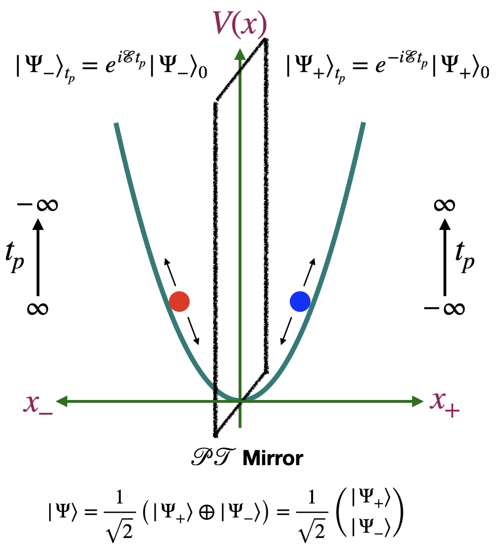
2. DQFT, in a Nutshell ()
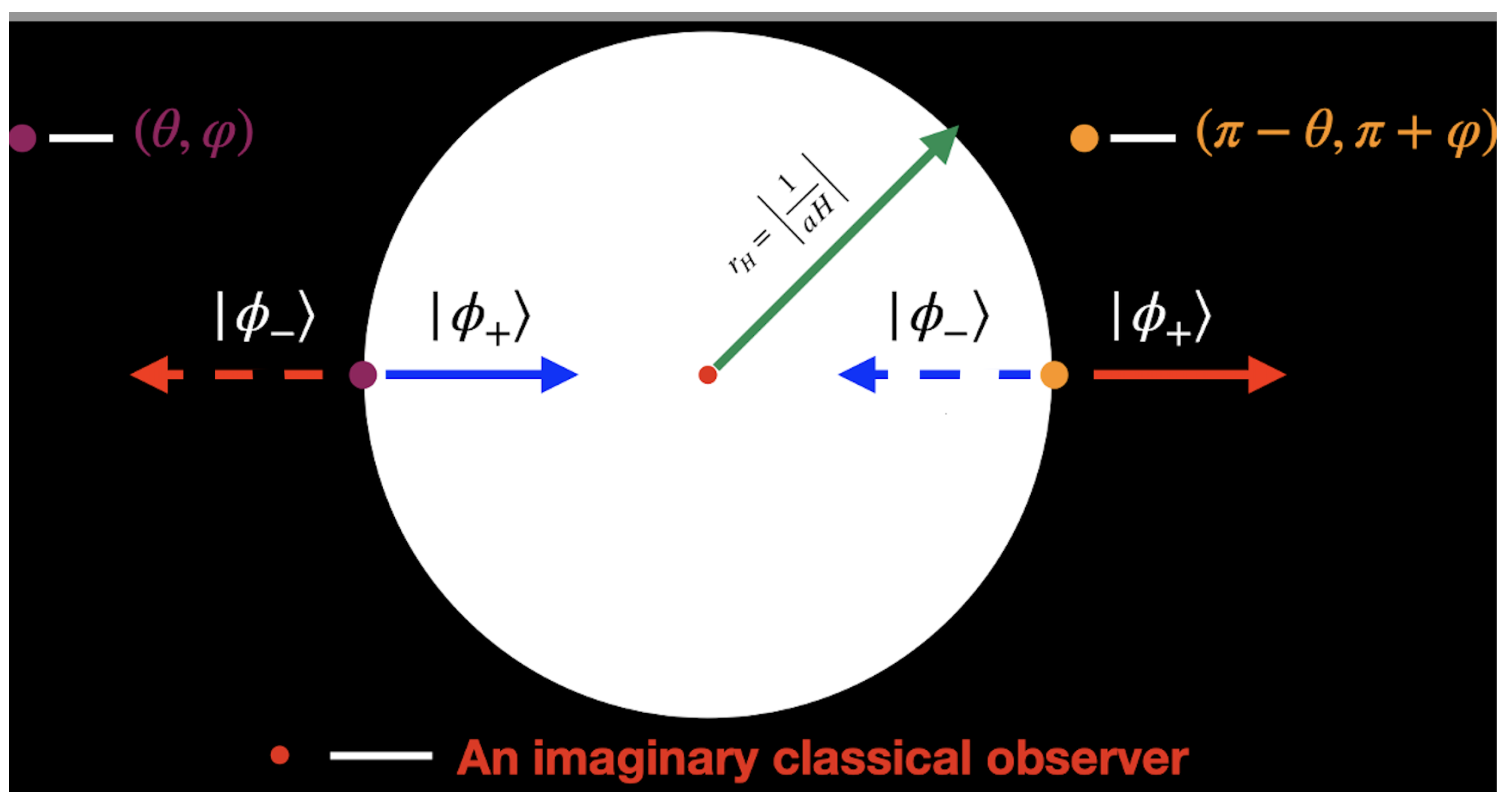
3. DQFT in de Sitter and Unitarity ()
4. CMB Parity Asymmetry
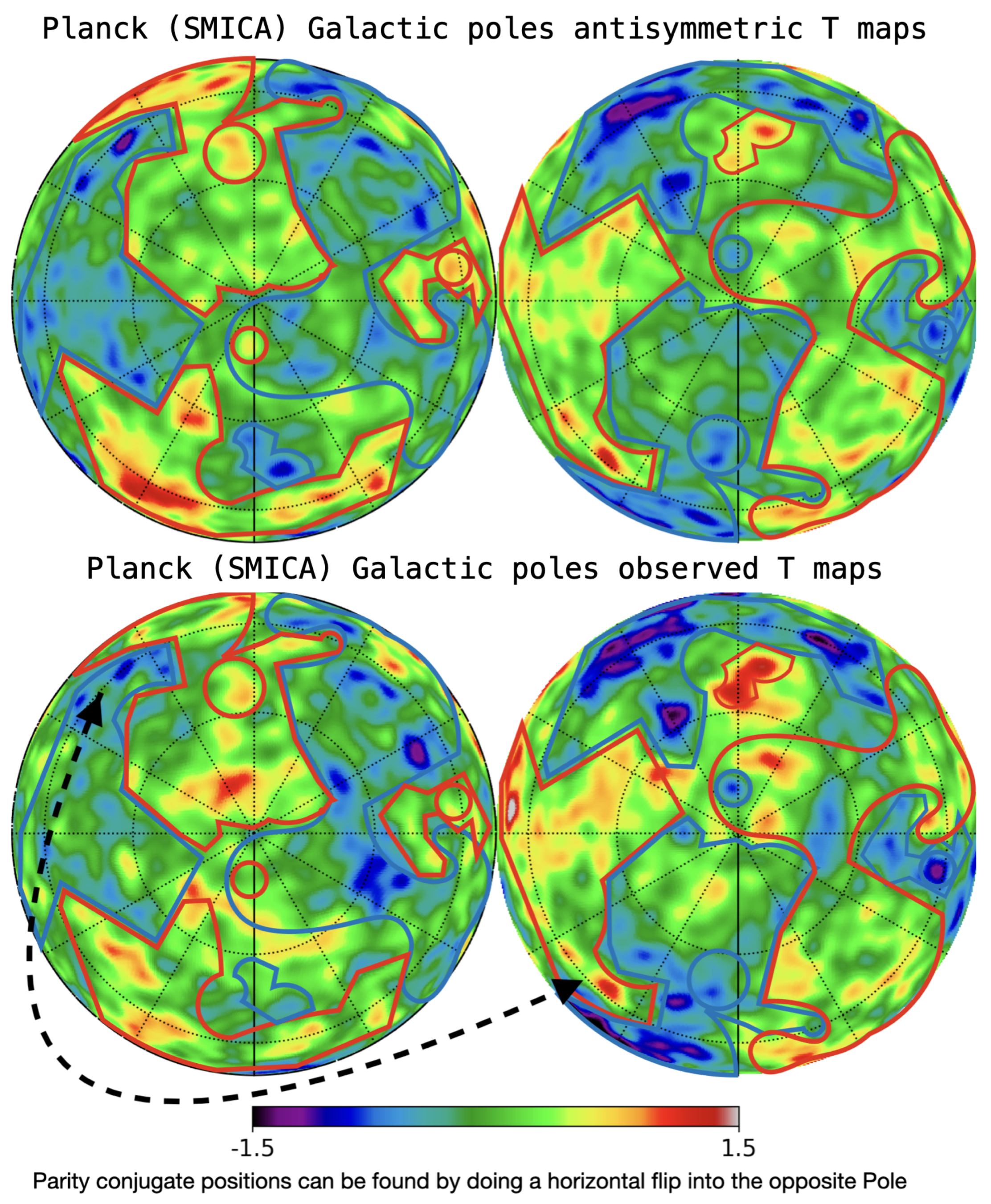
4.1. CMB Temperature Sky Fluctuations
4.2. DSI vs. SI Model Comparison and Simulations
5. Conclusions
Author Contributions
Funding
Data Availability Statement
Acknowledgments
Conflicts of Interest
Appendix A. Quantum Harmonic Oscillator in Direct-Sum Quantum Mechanics
Appendix B. Klein–Gordon Field Operator in DQFT
Appendix C. DQFT in dS
References
- Coleman, S. Lectures of Sidney Coleman on Quantum Field Theory; Chen, B.G., Derbes, D., Griffiths, D., Hill, B., Sohn, R., Ting, Y.-S., Eds.; WSP: Hackensack, NJ, USA, 2018. [Google Scholar] [CrossRef]
- Mukhanov, V.F.; Chibisov, G.V. Quantum Fluctuations and a Nonsingular Universe. J. Exp. Theor. Phys. Lett. 1981, 33, 532–535. [Google Scholar]
- Sasaki, M. Large Scale Quantum Fluctuations in the Inflationary Universe. Prog. Theor. Phys. 1986, 76, 1036. [Google Scholar] [CrossRef]
- Albrecht, A.; Ferreira, P.; Joyce, M.; Prokopec, T. Inflation and squeezed quantum states. Phys. Rev. D 1994, 50, 4807–4820. [Google Scholar] [CrossRef] [PubMed]
- Hawking, S.W. Black hole explosions. Nature 1974, 248, 30–31. [Google Scholar] [CrossRef]
- Hawking, S.W. Particle Creation by Black Holes. Commun. Math. Phys. 1975, 43, 199–220, Erratum in Commun. Math. Phys. 1976, 46, 206. [Google Scholar] [CrossRef]
- Gibbons, G.W.; Hawking, S.W. Cosmological Event Horizons, Thermodynamics, and Particle Creation. Phys. Rev. D 1977, 15, 2738–2751. [Google Scholar] [CrossRef]
- Schrodinger, E. Expanding Universes; Cambridge University Press: Cambridge, UK, 1956. [Google Scholar]
- Parikh, M.K.; Savonije, I.; Verlinde, E.P. Elliptic de Sitter space: DS/Z(2). Phys. Rev. D 2003, 67, 064005. [Google Scholar] [CrossRef]
- Parikh, M.K.; Verlinde, E.P. De Sitter holography with a finite number of states. J. High Energy Phys. 2005, 1, 54. [Google Scholar] [CrossRef]
- Almheiri, A.; Hartman, T.; Maldacena, J.; Shaghoulian, E.; Tajdini, A. The entropy of Hawking radiation. Rev. Mod. Phys. 2021, 93, 35002. [Google Scholar] [CrossRef]
- Hartman, T.; Jiang, Y.; Shaghoulian, E. Islands in cosmology. J. High Energy Phys. 2020, 11, 111. [Google Scholar] [CrossRef]
- Shaghoulian, E.; Susskind, L. Entanglement in De Sitter space. J. High Energy Phys. 2022, 8, 198. [Google Scholar] [CrossRef]
- Balasubramanian, V.; Horava, P.; Minic, D. Deconstructing de Sitter. J. High Energy Phys. 2001, 5, 43. [Google Scholar] [CrossRef]
- Balasubramanian, V.; Kar, A.; Ugajin, T. Entanglement between two gravitating universes. Class. Quant. Grav. 2022, 39, 174001. [Google Scholar] [CrossRef]
- Shaghoulian, E. The central dogma and cosmological horizons. J. High Energy Phys. 2022, 1, 132. [Google Scholar] [CrossRef]
- Giddings, S.B. The deepest problem: Some perspectives on quantum gravity. arXiv 2022, arXiv:2202.08292. [Google Scholar]
- ’t Hooft, G. Black hole unitarity and antipodal entanglement. Found. Phys. 2016, 46, 1185–1198. [Google Scholar] [CrossRef]
- Einstein, A.; Rosen, N. The Particle Problem in the General Theory of Relativity. Phys. Rev. 1935, 48, 73–77. [Google Scholar] [CrossRef]
- Kumar, K.S.; Marto, J.A. Towards a Unitary Formulation of Quantum Field Theory in Curved Spacetime: The Case of de Sitter Spacetime. Symmetry 2025, 17, 29. [Google Scholar] [CrossRef]
- Kumar, K.S.; Marto, J. Towards a Unitary Formulation of Quantum Field Theory in Curved Space-Time: The Case of the Schwarzschild Black Hole. Prog. Theor. Exp. Phys. 2024, 2024, 123E01. [Google Scholar] [CrossRef]
- Gaztañaga, E.; Kumar, K.S.; Marto, J. A New Understanding of Einstein-Rosen Bridges. Preprints 2024. [Google Scholar] [CrossRef]
- Kumar, K.S.; Marto, J.A. Hawking radiation with pure states. Gen. Rel. Grav. 2024, 56, 143. [Google Scholar] [CrossRef]
- Kumar, K.S.; Marto, J.A. Revisiting Quantum Field Theory in Rindler Spacetime with Superselection Rules. Universe 2024, 10, 320. [Google Scholar] [CrossRef]
- Gaztañaga, E.; Kumar, K.S. Finding origins of CMB anomalies in the inflationary quantum fluctuations. J. Cosmol. Astropart. Phys. 2024. [Google Scholar] [CrossRef]
- Kumar, K.S.; Marto, J. Parity asymmetry of primordial scalar and tensor power spectra. arXiv 2024, arXiv:2209.03928. [Google Scholar]
- Donoghue, J.F.; Menezes, G. Arrow of Causality and Quantum Gravity. Phys. Rev. Lett. 2019, 123, 171601. [Google Scholar] [CrossRef]
- Bender, C.M.; Boettcher, S.; Meisinger, P. PT symmetric quantum mechanics. J. Math. Phys. 1999, 40, 2201–2229. [Google Scholar] [CrossRef]
- Kiefer, C. Quantum Gravity, 2nd ed.; Oxford University Press: New York, NY, USA, 2007. [Google Scholar]
- Conway, J.B. A Course in Functional Analysis, 2nd ed.; Conway, J.B., Ed.; Graduate Texts in Mathematics; Springer Science+Business Media: New York, NY, USA, 2010; p. 96. [Google Scholar]
- Giulini, D. Superselection Rules. arXiv 2007, arXiv:0710.1516. [Google Scholar]
- nLab Authors. Superselection Theory. 2023. Available online: https://ncatlab.org/nlab/show/superselection+theory (accessed on 2 December 2024).
- Wick, G.C.; Wightman, A.S.; Wigner, E.P. The intrinsic parity of elementary particles. Phys. Rev. 1952, 88, 101–105. [Google Scholar] [CrossRef]
- Lanczos, K.; Hoenselaers, C. On a Stationary Cosmology in the Sense of Einstein’s Theory of Gravitation [1923]. GR Gravit. 1997, 29, 361–399. [Google Scholar]
- Hartman, T. Lecture Notes on Classical de Sitter Space. 2017. Available online: http://www.hartmanhep.net/GR2017/desitter-lectures-v2.pdf (accessed on 2 December 2024).
- Mukhanov, V.; Winitzki, S. Introduction to Quantum Effects in Gravity; Cambridge University Press: Cambridge, UK, 2007. [Google Scholar]
- ’t Hooft, G. Quantum Clones inside Black Holes. Universe 2022, 8, 537. [Google Scholar] [CrossRef]
- Boyle, L.; Finn, K.; Turok, N. CPT-Symmetric Universe. Phys. Rev. Lett. 2018, 121, 251301. [Google Scholar] [CrossRef]
- Boyle, L.; Finn, K.; Turok, N. The Big Bang, CPT, and neutrino dark matter. Ann. Phys. 2022, 438, 168767. [Google Scholar] [CrossRef]
- Sakharov, A.D. Violation of CP Invariance, C asymmetry, and baryon asymmetry of the universe. Pisma Zh. Eksp. Teor. Fiz. 1967, 5, 32–35. [Google Scholar] [CrossRef]
- Sakharov, A.D. Cosmological Models of the Universe With Rotation of Time’s Arrow. Sov. Phys. JETP 1980, 52, 349–351. [Google Scholar] [CrossRef]
- Gaztanaga, E. How the Big Bang Ends Up Inside a Black Hole. Universe 2022, 8, 257. [Google Scholar] [CrossRef]
- Gaztañaga, E. The mass of our observable Universe. Mon. Not. R. Astron. Soc. 2023, 521, L59–L63. [Google Scholar] [CrossRef]
- Gaztañaga, E.; Kumar, K.S.; Pradhan, S.; Gabler, M. Gravitational bounce from the quantum exclusion principle. Phys. Rev. D 2025, 111, 103537. [Google Scholar] [CrossRef]
- Starobinsky, A.A. A New Type of Isotropic Cosmological Models Without Singularity. Phys. Lett. 1980, B91, 99–102. [Google Scholar] [CrossRef]
- Baumann, D. Primordial Cosmology. Proc. Sci. 2018, 305. [Google Scholar] [CrossRef]
- Brunetti, R.; Fredenhagen, K.; Hoge, M. Time in quantum physics: From an external parameter to an intrinsic observable. Found. Phys. 2010, 40, 1368–1378. [Google Scholar] [CrossRef]
- Donoghue, J.F.; Menezes, G. Causality and gravity. J. High Energy Phys. 2021, 11, 10. [Google Scholar] [CrossRef]
- Roberts, B.W. Reversing the Arrow of Time; Cambridge University Press: Cambridge, UK, 2022. [Google Scholar] [CrossRef]
- Martin, J. Inflationary cosmological perturbations of quantum-mechanical origin. Lect. Notes Phys. 2005, 669, 199–244. [Google Scholar] [CrossRef]
- Akrami, Y.; Arroja, F.; Ashdown, M.; Aumont, J.; Baccigalupi, C.; Ballardini, M.; Banday, A.J.; Barreiro, R.B.; Bartolo, N.; Basak, S.; et al. Planck 2018 results. X. Constraints on inflation. Astron. Astrophys. 2020, 641, A10. [Google Scholar] [CrossRef]
- Komatsu, E. New physics from the polarized light of the cosmic microwave background. Nat. Rev. Phys. 2022, 4, 452–469. [Google Scholar] [CrossRef]
- Sachs, R.K.; Wolfe, A.M. Perturbations of a Cosmological Model and Angular Variations of the Microwave Background. Astrophys. J. 1967, 147, 73. [Google Scholar] [CrossRef]
- Durrer, R. The Cosmic Microwave Background; Cambridge University Press: Cambridge, UK, 2020. [Google Scholar] [CrossRef]
- Akrami, Y.; Ashdown, M.; Aumont, J.; Baccigalupi, C.; Ballardini, M.; Banday, A.J.; Barreiro, R.B.; Bartolo, N.; Basak, S.; Benabed, K.; et al. Planck 2018 results. VII. Isotropy and Statistics of the CMB. Astron. Astrophys. 2020, 641, A7. [Google Scholar] [CrossRef]
- Ashtekar, A.; Gupt, B.; Sreenath, V. Cosmic Tango Between the Very Small and the Very Large: Addressing CMB Anomalies Through Loop Quantum Cosmology. Front. Astron. Space Sci. 2021, 8, 76. [Google Scholar] [CrossRef]
- Kitazawa, N.; Sagnotti, A. String theory clues for the low–ℓ CMB ? EPJ Web Conf. 2015, 95, 3031. [Google Scholar] [CrossRef]


| Parity Indicator | SI | SI | DSI | Ratio DSI/SI |
|---|---|---|---|---|
| 2.62% | 0.09% | 3.3% | 37 | |
| 1.0% | 0.7% | 39.5% | 56 | |
| 3.89% | 1.12% | 45.3% | 40 | |
| 0.12% | 0.003% | 1.96% | 653 | |
| 0.45% | 34.6% | 77 | ||
| 0.016% | 2.65% | 166 |
Disclaimer/Publisher’s Note: The statements, opinions and data contained in all publications are solely those of the individual author(s) and contributor(s) and not of MDPI and/or the editor(s). MDPI and/or the editor(s) disclaim responsibility for any injury to people or property resulting from any ideas, methods, instructions or products referred to in the content. |
© 2025 by the authors. Licensee MDPI, Basel, Switzerland. This article is an open access article distributed under the terms and conditions of the Creative Commons Attribution (CC BY) license (https://creativecommons.org/licenses/by/4.0/).
Share and Cite
Gaztañaga, E.; Kumar, K.S. CMB Parity Asymmetry from Unitary Quantum Gravitational Physics. Symmetry 2025, 17, 1056. https://doi.org/10.3390/sym17071056
Gaztañaga E, Kumar KS. CMB Parity Asymmetry from Unitary Quantum Gravitational Physics. Symmetry. 2025; 17(7):1056. https://doi.org/10.3390/sym17071056
Chicago/Turabian StyleGaztañaga, Enrique, and K. Sravan Kumar. 2025. "CMB Parity Asymmetry from Unitary Quantum Gravitational Physics" Symmetry 17, no. 7: 1056. https://doi.org/10.3390/sym17071056
APA StyleGaztañaga, E., & Kumar, K. S. (2025). CMB Parity Asymmetry from Unitary Quantum Gravitational Physics. Symmetry, 17(7), 1056. https://doi.org/10.3390/sym17071056