Modeling Temporal Symmetry: Dual-Component Framework for Trends and Fluctuations in Time Series Forecasting

Abstract

Time-series forecasting is a cornerstone of decision making in domains such as finance, energy management, and meteorology, where precise predictions drive both economic and operational efficiency. However, traditional time-domain methods often struggle to capture the intricate symmetries and hierarchical dependencies inherent in complex multivariate time-series data. These methods frequently fail to distinguish between global trends and localized fluctuations, limiting their ability to model the multifaceted temporal dynamics that arise across different time scales. To address these challenges, we propose a novel dual-component framework that explicitly leverages the symmetry between long-term trends and short-term fluctuations. Inspired by the principles of signal decomposition, we partition time-series data into a low-frequency stabilization component and a high-frequency fluctuation component. The stabilization component captures inter-variable relationships and global frequency-domain component dependencies through Fourier-transformed frequency-domain representations, variable-oriented attention mechanisms, and dilated causal convolutions. Meanwhile, the fluctuation component models localized dynamics using a multi-granularity structure and time-step attention mechanisms to enhance the sensitivity and robustness to transient variations. By integrating these complementary perspectives, our approach provides a more holistic representation of time-series dynamics. Comprehensive experiments on benchmark datasets from electricity, transportation, and weather domains demonstrate that our method consistently outperforms state-of-the-art models, achieving superior accuracy. Beyond predictive performance, our framework offers a deeper interpretability of temporal behaviors, highlighting its potential for practical applications in complex systems. This work underscores the importance of symmetry-aware modeling in advancing time-series forecasting methodologies.

1. Introduction

Multivariate time-series forecasting is a cornerstone of modern decision-making in domains such as power energy management [1], traffic flow prediction [2], weather forecasting [3,4], disease transmission monitoring [5], and financial market analysis [6,7]. The ability to accurately predict future trends based on historical data is critical for optimizing resources, mitigating risks, and enabling proactive planning. However, multivariate time-series data are inherently complex, often characterized by nonlinear dynamics, intricate temporal dependencies, and multiscale patterns. These challenges make effective modeling not only a technical necessity but also a scientific frontier [8,9].

Traditional machine learning methods, such as linear regression, support vector machines, and decision trees, have been widely applied to time-series forecasting due to their simplicity and interpretability [10,11,12,13]. However, their reliance on strong assumptions such as linearity or independent and identically distributed data limits their ability to capture the nonlinear interactions and temporal correlations that define real-world systems. These methods are often constrained to extracting local features, failing to provide a holistic understanding of global dynamics or long-term dependencies.

The advent of deep learning has revolutionized time-series forecasting by enabling models to learn complex patterns directly from data [14,15,16,17]. Recurrent neural networks (RNNs) [14,18,19], convolutional neural networks (CNNs) [20,21,22], and Transformer-based models [23,24] have demonstrated remarkable success in capturing temporal dependencies. RNNs excel at sequential modeling but often suffer from vanishing gradients and inefficiencies in handling long sequences. CNNs, with their ability to extract local features efficiently, require deep architectures to model long-range dependencies, leading to increased computational complexity. Transformers, leveraging attention mechanisms, overcome these limitations by modeling dependencies across any two time steps, significantly enhancing the understanding of long-distance relationships. Despite these advances, most existing methods still heavily rely on the modeling of time steps under a time-domain representation, which, although intuitive, often fails to capture the spectral relationships, multivariate dependencies, and dynamic interactions between long-term trends and high-frequency fluctuations inherent in real-world time-series data.

Time-series data exhibit a natural duality: they are governed by both long-term trends that reflect global stability and short-term fluctuations that capture transient dynamics. This duality suggests an inherent symmetry between global and local behaviors, where each component complements the other to form the complete temporal structure. In other words, the two components interact to form the sequential relationship in the time series, and when the series fluctuates sharply beyond expectations, it is a ‘manifestation of imbalance’, whilst the work of time-series forecasting can also be interpreted as finding the ‘balance and symmetry relationship’ in the series. For example, in energy management, long-term trends may represent seasonal patterns, while short-term fluctuations capture daily variations. Similarly, in financial markets, global trends might indicate overall economic growth, while local fluctuations reflect market volatility. Existing methods, however, often fail to explicitly model this symmetry, treating time series as either a monolithic sequence or focusing disproportionately on one aspect, such as global trends or local variations. This imbalance limits their ability to fully exploit the complementary nature of these dynamics, leading to suboptimal forecasting performance.

To address these challenges, we propose a symmetry-aware framework for multivariate time-series forecasting that explicitly leverages the complementary relationship between long-term trends and short-term fluctuations. Inspired by the natural balance between stability and variability in time series, our framework decomposes the input data into two distinct components: a low-frequency stabilization term and a high-frequency fluctuation term. This decomposition reflects the inherent symmetry between global and local dynamics, enabling specialized modeling for each component. The stabilization term captures overarching long-term trends and frequency-domain component dependencies through Fourier-enhanced frequency-domain representations, variable-oriented attention mechanisms, and causal dilated convolutions. By operating in the frequency domain, this component provides a compact and interpretable representation of global patterns, bridging forward and near-term dependencies. Meanwhile, the fluctuation term focuses on capturing local dynamics in the time domain, using a temporal multi-granularity structure and a time-step focusing mechanism to model intricate short-term changes. This dual-component design ensures that both global stability and local variability are effectively captured, enhancing the model’s ability to forecast across multiple time scales. Our approach is validated on benchmark datasets from diverse domains, including electricity, transportation, and meteorology. Experimental results demonstrate significant improvements in forecasting accuracy compared to the state-of-the-art models. Beyond its predictive performance, our framework provides deeper interpretability by offering distinct representations of long-term and short-term dynamics, aligning with the natural symmetry observed in real-world systems.

Our main contributions are summarized as follows:

• We propose a novel framework that explicitly leverages the symmetry between long-term trends and short-term fluctuations in time series. By decomposing the data into low-frequency stabilization and high-frequency fluctuation components, our method captures the complementary dynamics inherent in multivariate time series.
• The stabilization term is modeled using Fourier-enhanced frequency-domain representations, multivariate attention mechanisms, and causal dilated convolutions, providing a global view of the time dynamics underlying the low-frequency components in the frequency domain. This integration bridges the gap between frequency-domain and time-domain analyses, offering a more holistic understanding of time series.
• The fluctuation terms are handled using a multi-granularity approach in which short-term changes are constructed over multiple time scales, ensuring sensitivity and robustness. Coupled with a time-step attention mechanism, this design ensures the precise modeling of local dynamics and transient changes.
• Our framework achieves state-of-the-art predictive accuracy on benchmark datasets through the efficient modeling of trends and fluctuations. As such, it is particularly well suited for real-world applications that require precision and insight.

This paper is organized as follows: Section 2 presents related work; Section 3 describes the proposed model architecture; Section 4 discusses experimental results and analysis; Section 5 concludes the paper and outlines future research directions.

2. Related Work

As shown in Figure 1, the mainstream approach of the frequency-domain perspective, the attention mechanism, and convolution in the field of time-series forecasting are demonstrated, respectively.

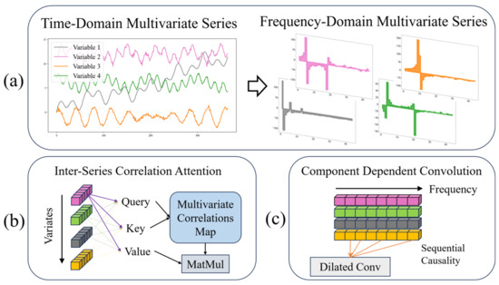
Figure 1. Several mainstream approaches in multivariate time-series forecasting, (a) transformation between time and frequency-domain perspectives, with colored squares representing the frequency-domain magnitude of each feature; (b) attention mechanisms oriented towards multivariate interactions, with colored squares representing the time step of each feature; (c) dilated causal convolution in the frequency domain, with colored squares representing the frequency component of each feature.

2.1. Frequency-Domain Perspective Methods

Frequency-domain analysis is an essential tool in time-series forecasting, adept at handling tasks such as selecting frequency components, computing spectral data, reducing noise, and identifying periodic patterns. Existing studies frequently leverage frequency-domain methods to enhance time-series prediction models. Techniques such as the Fourier transform are utilized to capture periodic patterns, expedite computation, and analyze spectral sparsity. Traditional spectral density methods further contribute by examining how power is distributed across different frequencies. These methods decompose time series into sinusoidal components, facilitating the identification of dominant cycles and periodicities that may not be evident in the time domain [25]. By estimating spectral density, researchers can effectively isolate and model long-range dependencies and persistent cycles, crucial for improving the forecast accuracy in complex datasets [26].

In the recently popular deep learning methods, autoformer [27] utilizes the Wiener–Khinchin theorem to model long-term dependencies by capturing periodic similarities through the fast Fourier transform (FFT). However, it primarily focuses on phase changes in similar sub-processes without adequately addressing the interactions among variables in multivariate time series. FEDformer [28] enhances computational efficiency in processing large-scale data by assuming spectral sparsity and selectively analyzing random frequency components. Nevertheless, this approach may overlook non-periodic and mixed frequency features, thus compromising the modeling of complex dependencies in multivariate time series. The FITS model [29] employs complex-valued linear neural networks to generate frequency-domain representations, making it suitable for deployments on resource-constrained edge devices. Despite its efficiency, FITS struggles with nonlinear dependencies and complex interactions among variables. TimesNet [30] identifies primary periodic patterns using FFT and integrates them with convolutional networks to model periodic behaviors. However, it remains inadequate for handling non-periodic signals and their interactions among variables. FNet [31] replaces traditional attention mechanisms with a parameter-free Fourier transform, significantly boosting GPU computational efficiency but still falling short in capturing both long- and short-term dependencies and complex spatio-temporal interactions. FiLM [32] merges Fourier analysis with low-rank matrix approximation to improve noisy signal processing, yet it primarily focuses on noise reduction and spectral sparsity, lacking in its ability to model the intricate dynamics of dependencies in multivariate time series.

While these methods have advanced time-series forecasting by focusing on identifying periodic patterns and enhancing computational efficiency, they generally do not exploit the combined analysis of frequency and time domains to fully capture the complex dependencies in multivariate time series. Frequency-domain analysis should be integrated with time-domain information to more comprehensively capture dynamic characteristics across different time scales. Current models often treat frequency components as isolated analytical objects, overlooking the synergies among different frequency components and the interdependencies among variables, which are crucial for the improving prediction accuracy in multivariate time series. Our study addresses these shortcomings by decomposing the time series into a low-frequency stable term and a high-frequency fluctuation term, targeting both long-term trends and short-term fluctuations. By jointly modeling in both the frequency and time domains, our approach effectively captures the interactions among variables and enhances the accuracy of long-term forecasts.

2.2. Attention Mechanism Methods

Since the inception of the transformer model, it has significantly impacted fields like natural language processing and computer vision, primarily due to its multi-head self-attention mechanism which adeptly captures long-range dependencies [23]. Recently, transformers have also been adapted for time-series forecasting, particularly for modeling extended series. However, most existing Transformer-based methods predominantly focus on dependencies between time steps, often overlooking the critical capture of multi-frequency characteristics and complex interactions among variables in multivariate time series. Informer [24] effectively enhances the computational efficiency and manages long time-series data using the ProbSparse self-attention mechanism and a generative decoder strategy. Yet, it primarily addresses semantic dependencies between time steps without fully considering the variable interactions in multivariate contexts. Similarly, LogTrans [33] introduces a sparse attention mechanism that uses exponentially spaced time steps to decrease memory and time requirements. Although this improves computational efficiency, it continues to focus on sparse time-step dependencies, neglecting cross-variable interactions. To bridge these gaps, Autoformer [27] and FEDformer [28] incorporate the autocorrelation mechanisms and Fourier augmentation blocks, respectively, aiming to enhance long-range dependency modeling through frequency–domain information. Despite these advancements, their handling of frequency-domain processing primarily accelerates computation and captures periodic features without fully exploring multi-frequency components and inter-variable dependencies. Pyraformer [34] employs a pyramid attention mechanism to capture multiscale temporal dependencies, which is beneficial for processing long series. However, it still primarily focuses on time-step dependencies, overlooking the interactions between different frequency characteristics. Recent models like iTransformer [35] improve the capture of multivariate dependencies by assigning each variable a separate high-dimensional feature representation, moving away from the traditional Transformer focus on time-step dependencies alone. Nonetheless, these models often process all variables at the same time-step marker, which limits their ability to capture complex interactions among variables, thus constraining comprehensive modeling of multi-frequency, multivariate time series. PatchTST, a novel Transformer variant, segments a time series into localized patches—similar to the Vision Transformer’s approach in computer vision—to capture both local and global temporal dependencies [36]. Although effective in long time-series prediction, its exploration of multi-frequency components and cross-variable dependencies remains superficial. TCDformer [37] and TimeXer [38] focus on enhancing temporal consistency and processing efficiency but still face limitations in addressing frequency components and inter-variable dependencies, despite employing mechanisms like the local linear scaling approximation (LLSA) for non-stationary series.

Despite advancements in modeling time-step dependencies and optimizing computational efficiency, existing Transformer variants often neglect the crucial role of frequency dependency in multivariate time series. This oversight, coupled with the embedding of multiple variables in the same time-step marker, complicates the efficient capture of complex variable interactions. This often leads to an ineffective representation of the attention mechanism and fails to fully delineate the intricate dynamics in multivariate time series. Addressing these deficiencies, our study proposes a novel approach that integrates frequency domain analysis with attention mechanisms, decomposing the time series into a low-frequency stable term and a high-frequency fluctuating term. The low-frequency stable term captures long-range frequency dependencies using a combination of Fourier enhancement and attention mechanisms, while the high-frequency fluctuating term leverages a time-domain attention mechanism to enhance the capture of local fluctuations and short-term dependencies. Compared to existing models, our method not only addresses the challenges of modeling multiple frequency components and complex interactions among variables but also offers a more holistic framework for time-series forecasting, providing a global perspective on the dynamic properties of different frequency components.

2.3. Sequence Decomposition Methods

Sequence decomposition is a fundamental technique in time-series forecasting, aiming to disentangle complex temporal data into distinct components such as trends, seasonality, and irregular fluctuations. By isolating these components, decomposition methods improve both predictive accuracy and interpretability. Recent works have demonstrated the effectiveness of decomposition in handling diverse temporal dynamics and enhancing model robustness.

In the classical approach, ARIMA (autoregressive integrated moving average) models have traditionally been employed to capture linear dependencies and short-term correlations within decomposed components. ARIMA models are characterized by their ability to model non-stationary data through differencing, autoregressive terms, and moving averages, making them versatile for various applications [39]. However, for time series exhibiting long memory or persistent temporal dependencies, ARFIMA (autoregressive fractionally integrated moving average) models provide a more sophisticated approach. ARFIMA extends ARIMA by incorporating fractional differencing, allowing it to model long-range dependencies more effectively [40].

In the recently popular deep learning methods, Autoformer [27] introduces a decomposition sub-module based on moving averages, separating time series into trend and seasonal components. This allows the model to focus on stable global patterns and recurring local fluctuations. Building on this, FEDformer [28] incorporates multicore moving averages to enable multiscale decomposition, capturing complex temporal dynamics across different resolutions. Similarly, DLinear [41] employs decomposition as a preprocessing step, isolating trend, and seasonal components to simplify forecasting for linear regression models.

In frequency-domain decomposition and frequency processing preferences, the Holt–Winters triple exponential smoothing method is a classical technique that focuses on capturing low-frequency trends and seasonal components, making it suitable for handling long-term changes and stable patterns [42]. In contrast, long short-term memory networks (LSTMs), a variant of recurrent neural networks, excel at processing high-frequency data, making it particularly adept at analyzing time series with rapid fluctuations and short-term patterns [43].

Further advancements include MICN [44], which combines decomposition with hybrid modeling by splitting input series into trend and seasonal components and integrating global and local forecasts to adapt to dynamic changes [45,46]. DFNet [47] extends decomposition further with a three-branch structure to separate trend, seasonal, and irregular components, explicitly modeling noise and unpredictable fluctuations for improved robustness in volatile datasets.

While existing methods effectively leverage decomposition to isolate temporal components, they often overlook the symmetry inherent in time-series data—the complementary relationship between global trends and local fluctuations. In real-world systems, trends provide long-term stability, while fluctuations capture transient dynamics, and both components work together to reconstruct the original series. This natural balance, or functional symmetry, is rarely modeled explicitly, leaving room for improvement in capturing the interplay between these components.

3. Methodology

3.1. Overview of the Structure

To address the challenges of multivariate long-term time-series forecasting, the proposed model adopts a dual-branch architecture based on frequency-temporal decomposition. This framework explicitly separates the input sequence into two complementary components: a low-frequency stable component and a high-frequency fluctuation component. This decomposition reflects the natural complementarity in time-series data, where long-term trends and short-term dynamics work together to form the overall temporal structure. By independently modeling these two components, the framework captures both global stability and local variability, enhancing forecasting accuracy and interpretability. The overall structure of the model is illustrated in Figure 2.

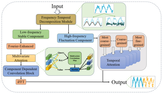
Figure 2. The overall framework of the proposed method. The known sequence as input is firstly divided into stable trend term and high frequency fluctuation term by decomposition module; the stable trend term is sequentially modeled in the frequency domain by Fourier augmentation, variable oriented attention (explained by the light green square expansion), and component-dependent convolution block; the high frequency fluctuation term is constructed in the time domain with multiple granularities, respectively, modeled by time-step Attention, and then integrated into the uniform size. The last two items are mixed for output.

The input time series is first processed by the frequency-temporal decomposition module, which decomposes the sequence into the low-frequency stable component and the high-frequency fluctuation component. These two components are then processed through distinct modeling pipelines tailored to their respective characteristics. The low-frequency stable component captures long-term trends and global patterns, while the high-frequency fluctuation component focuses on short-term dynamics and fine-grained variations. The outputs of these two branches are finally integrated through a projection layer to produce the unified forecast.

The low-frequency stable component is processed through a series of operations designed to extract long-term trends and global patterns. The first step involves transforming the stable component into the frequency domain using the Fourier transform. This transformation enables the model to analyze global patterns in a compact frequency-domain representation, where long-term trends are naturally emphasized. To enhance the extraction of meaningful patterns, a Fourier-enhanced block is applied to streamline the representation and focus on key frequency components. After the frequency-domain transformation, the stable component is passed through a variable-oriented multivariate attention mechanism, which models complex dependencies among the input variables. Unlike traditional attention mechanisms that primarily focus on temporal relationships, this module is designed to capture inter-variable correlations in the frequency domain, providing a deeper understanding of the global dynamics across multivariate time series. Following the attention-based modeling, the stable component undergoes further refinement through a Component Dependent Convolution Block, which combines causal convolution and dilation convolution. Causal convolution ensures the order of frequency-domain components from low to high is preserved, maintaining the causal structure of the data. Dilation convolution expands the receptive field exponentially, enabling the model to capture long-term dependencies and multiscale temporal patterns efficiently. Finally, the refined stable component is converted back to the time domain using an inverse Fourier transform, producing the predicted output for the low-frequency stable component.

The high-frequency fluctuation component, in contrast, focuses on short-term variations and fine-grained dynamics of the time series. To handle these transient and localized patterns, the fluctuation component is processed through a multi-granularity modeling pipeline. The fluctuation component is first decomposed into multiple granularities, including most coarse-grained, intermediate-grained, and most fine-grained representations. Each granularity captures features at a specific temporal resolution, enabling the model to address short-term dynamics across multiple time scales. Each granularity is then modeled independently using a temporal attention mechanism, which captures local dependencies and abrupt changes within the corresponding time scale. This mechanism ensures that fine-grained variations are effectively incorporated into the short-term forecast. After processing each granularity, the outputs are aggregated to produce a comprehensive prediction for the high-frequency fluctuation component. Although the fluctuation component represents a smaller portion of the time series, it plays a critical role in refining the forecast by capturing high-frequency changes that are often overlooked in traditional models. By combining the global perspective of the stable component with the local sensitivity of the fluctuation component, the model achieves a balanced and nuanced understanding of the time series.

The outputs of the low-frequency stable component and the high-frequency fluctuation component are combined through a projection layer to produce a unified forecast that integrates both long-term trends and short-term dynamics. This integration reflects the natural symmetry in time-series data, where the stable component provides a global perspective, and the fluctuation component refines the forecast with localized variations. By leveraging the frequency-temporal decomposition module, the model effectively separates and specializes its modeling of these complementary components. The Fourier-enhanced frequency modeling, multivariate attention mechanism, component dependent convolution block, and multi-granularity temporal attention work together to capture the intricate dependencies and multiscale dynamics inherent in multivariate time series.

3.2. Frequency-Temporal Decomposition and Fourier-Enhanced Block

3.2.1. Frequency-Temporal Decomposition

The proposed model begins by applying a frequency-temporal decomposition to the input time series, effectively separating it into a low-frequency stable component and a high-frequency fluctuation component. This separation allows the for specialized modeling of long-term trends and short-term dynamics, enhancing the overall forecasting accuracy.

Given a multivariate time-series input $\mathbf{X}\in {\mathbb{R}}^{T\times N}$, where T is the length of the series and N is the number of variables, the decomposition process involves transforming the series into the frequency domain using the discrete Fourier transform (DFT):

$${\widehat{x}}_n\left(f\right)=\sum _{t=0}^{T-1}{x}_n\left(t\right)e^{-j2\pi ft/T},f=0,1,\dots ,T-1,$$

(1)

where ${\widehat{x}}_n\left(f\right)$ denotes the frequency-domain representation for the n-th variable. This transformation results in $\widehat{\mathbf{X}}\in {\mathbb{C}}^{T\times N}$, capturing both the amplitude and phase information of the series.

The low-frequency stable component is extracted by applying a frequency mask $\mathbf{M}$, which emphasizes the low-frequency components while attenuating high-frequency noise. The filtered frequency representation is:

$${\widehat{\mathbf{X}}}_{\mathrm{low}}=\mathbf{M}\odot \widehat{\mathbf{X}},$$

(2)

where ⊙ denotes element-wise multiplication. The mask $\mathbf{M}$ is designed to prioritize frequencies near zero, effectively isolating long-term trends.

3.2.2. Fourier-Enhanced Block

The Fourier-Enhanced Block is a crucial part of the pipeline for modeling the low-frequency stable component, focusing on extracting and enhancing key patterns that represent long-term trends. This block operates in the frequency domain to provide a compact and informative representation of the stable component.

The Fourier-enhanced block involves two key operations: frequency selection and adaptive enhancement. Instead of using a fixed frequency mask, we introduce a learnable frequency gating mechanism. This mechanism dynamically selects relevant frequencies by using a parameterized function $\mathbf{G}\left(f\right)$, which is optimized during training:

$${\widehat{\mathbf{X}}}_{\mathrm{selected}}=\mathbf{G}\left(f\right)\odot \widehat{{\mathbf{X}}_{\mathbf{low}}},$$

(3)

where $\mathbf{G}\left(f\right)$ is a learnable gating function that adjusts the emphasis on different frequencies based on the data characteristics.

After frequency selection, the enhanced frequency components are further processed through a learnable transformation matrix ${\mathbf{W}}_F$:

$${\widehat{\mathbf{X}}}_{\mathrm{enhanced}}={\mathbf{W}}_F{\widehat{\mathbf{X}}}_{\mathrm{selected}}.$$

(4)

This matrix is trained to highlight significant patterns and suppress noise, allowing the model to adaptively focus on informative features.

3.3. Attention-Based Multivariate Modeling Module

In our multivariate time-series forecasting model, the attention-based multivariate modeling module is a key component for capturing multivariate frequency dependencies. This module is based on the classical self-attention mechanism in the Transformer framework and is modified to focus on capturing frequency dependencies and dynamic interactions among different variables. Unlike the traditional time-step dependency-based approach in time-series modeling, our approach treats the frequency components of each variable as independent processes and focuses on the frequency interactions among multi-variables through the self-attention mechanism.

3.3.1. Variable-Oriented Attention Mechanism

The self-attention mechanism is a pivotal operation within the Transformer framework, traditionally employed to capture both long-term and short-term dependencies in time-series data. Typically, this mechanism constructs time-step relationships in a time series by assessing the similarity between queries (Q), keys (K), and values (V). However, our model deviates from the traditional approach by treating the frequency series of each variable as interacting target features, thus capturing the interdependencies between different variables through a self-attention mechanism.

Consider a time series $H_{t_1:t_l}=\{h_{t_1},h_{t_2},\dots ,h_{t_l}\}$, representing sequence features extracted from the input data. We begin by mapping this sequence to queries (Q), keys (K), and values (V) via linear projections:

$$Q=H_{t_1:t_l}{W}_Q,K=H_{t_1:t_l}{W}_K,V=H_{t_1:t_l}{W}_V$$

(5)

where $W_Q,W_K,$ and $W_V$ are projection matrices, and $Q,K,V\in {\mathbb{R}}^{N\times d_k}$. Here, N represents the number of variables, and $d_k$ denotes the dimension of the hidden layer. The self-attention mechanism computes an attention weight matrix by assessing the similarity between Q and K. This attention matrix is then used to weight the value matrix V, effectively capturing the dependencies among variables. The formula for the attention mechanism is:

$$A\left(Q,K,V\right)=\mathrm{Softmax}\left({\displaystyle \frac{Q{K}^T}{\sqrt{d_k}}}\right)V$$

(6)

where the softmax activation function is used to normalize the attention score, ensuring a total weight of 1. Specifically, the query and key similarity $A_{i,j}$ is obtained by the inner product calculation:

$$A_{i,j}\propto {\displaystyle \frac{q_i^T{k}_j}{\sqrt{d_k}}}$$

(7)

This attention score $A_{i,j}$ reflects the correlation between different variables, i.e., the strength of the interaction of each variable at different time steps. Unlike traditional models, our self-attention mechanism focuses on capturing dependencies between multiple variables, not just between time steps. With this approach, the model is better able to identify the interactions of different variables in the frequency dimension and assign higher weights to the more relevant variables.

3.3.2. Variable-Oriented Layer Normalization

In order to improve the stability and convergence of the model, we introduce Variable LayerNorm in the inter-series correlation attention block, which is an improvement of the standard LayerNorm proposed by researchers [48,49,50]. The traditional LayerNorm normalizes all variables at the same time step in the Transformer model, but this approach may lead to the blurring of dependencies between different variables and cannot effectively capture multivariate features.

In our design, LayerNorm is applied to the time series of each variable to ensure that the independent characteristics of each variable are preserved, thus avoiding mutual interference between variables. The specific formula is as follows:

$$\mathrm{VariableLayerNorm}\left(X\right)={\displaystyle \frac{x_n-\mathrm{Mean}\left(x_n\right)}{\sqrt{\mathrm{Var}\left(x_n\right)}}},n=1,\dots ,N.$$

(8)

By normalizing the series of each variable, the model is able to effectively deal with the challenges posed by non-stationary data, reduce errors due to measurement inconsistency, and prevent the problem of over-smoothing of the series that may be introduced by traditional normalization. Compared to traditional methods, this variable-based normalization strategy enhances the predictive power of the model by maintaining the temporal pattern of each variable and avoiding the introduction of unwanted interaction noise between different time steps.

This approach is particularly effective in dealing with non-stationary multivariate time series with dynamically changing characteristics, as traditional standardization strategies often fail to accommodate statistical properties that vary over time. By dynamically adjusting the time-series representation of each variable, our model ensures higher robustness and adaptability to capture frequency dependence and complex variable interactions.

3.4. Convolution-Based Frequency Component Modeling Module

Our proposed architecture is based on temporal convolutional networks [22,51] for sequential modeling of the frequency components of time series. Unlike traditional complex convolutional designs (context stacking, or gated activation [52]), our approach aims to maintain simplicity and low complexity while enabling the memorization and processing of very long time series.

The component dependent convolution block (CDCB) is designed to refine the low-frequency stable component by capturing the interactions between low-frequency trends and their high-frequency harmonics. This block employs a novel causal convolution approach in the frequency domain, ensuring that the modeling sequence respects the inherent hierarchy from low to high frequencies.

In the CDCB, causal convolution is adapted to operate in the frequency domain, focusing on the sequential relationship from low to high frequencies. This approach models how lower frequencies influence higher frequencies, reflecting the natural dependency structure where high-frequency components can incorporate information from low-frequency trends.

Given the frequency-domain representation ${\widehat{\mathbf{X}}}_{\mathrm{stable}}\in {\mathbb{C}}^{T\times N}$, the causal convolution is defined as:

$${\widehat{y}}_n\left(f\right)=\sum _{k=0}^{K-1}{w}_k{\widehat{x}}_n(f-k),$$

(9)

where $f-k\ge 0$ ensures that each frequency component ${\widehat{y}}_n\left(f\right)$ only depends on lower or equal frequencies, thus maintaining causality in the frequency domain.

To capture the nuanced interactions between different frequency bands, the CDCB employs a hierarchical approach where convolutional layers are stacked with increasing dilation factors. This setup allows the block to model both immediate and distant harmonic relationships efficiently:

1. Base layer: Models direct influences of low-frequency components on nearby harmonics.

2. Dilated layers: Use dilation to expand the receptive field, capturing broader interactions across the frequency spectrum.

It gradually captures the expanded frequency relationships without incurring excessive computational costs.

To enhance the flexibility of the CDCB, an adaptive frequency filtering mechanism is integrated. This mechanism dynamically adjusts the emphasis on different frequency bands based on the data characteristics. A learnable filter $\mathbf{F}\left(f\right)$ is applied:

$${\widehat{\mathbf{X}}}_{\mathrm{filtered}}=\mathbf{F}\left(f\right)\odot {\widehat{\mathbf{X}}}_{\mathrm{stable}},$$

(10)

where $\mathbf{F}\left(f\right)$ is optimized to highlight the significant frequencies and suppress noise, allowing the model to focus on the most informative harmonic interactions.

Subsequently, the refined frequency-domain representation from the CDCB is transformed back to the time domain using the inverse Fourier transform. This time-domain signal incorporates both the global trends and the subtle harmonic variations, providing a comprehensive representation of the stable component.

3.5. Multi-Granularity Temporal Modeling Module

The multi-granularity temporal modeling module is designed to model the high-frequency fluctuation component of a time series by capturing its short-term dynamics across multiple temporal scales. High-frequency components often involve complex and transient variations that are difficult to capture using a single temporal resolution. To address this, the module employs a multi-granularity approach combined with a time-step attention mechanism, enabling the model to analyze and synthesize information from various granularities. This design allows the module to adaptively focus on relevant time steps and their relationships, ensuring a precise representation of high-frequency dynamics.

3.5.1. Multi-Granularity Decomposition

The first step in the module is to decompose the high-frequency fluctuation component into multiple granularities, each representing the sequence at a different temporal resolution. This decomposition is achieved by downsampling the original time series ${\mathbf{X}}_{\mathrm{fluctuation}}\in {\mathbb{R}}^{T\times N}$ using different aggregation windows. Specifically, for a granularity level m, the sequence is divided into non-overlapping segments of size $w_m$, where $w_m$ represents the window size for that granularity. The value of $w_m$ determines the scale of temporal resolution, with larger $w_m$ corresponding to coarser granularities. The down-sampled sequence at granularity m is computed as:

$${\mathbf{X}}_g^m\left[t\right]={\displaystyle \frac{1}{w_m}}\sum _{k=0}^{w_m-1}{\mathbf{X}}_{\mathrm{fluctuation}}[t·w_m+k],t=0,1,\dots ,⌊{\displaystyle \frac{T}{w_m}}⌋-1,$$

(11)

where ${\mathbf{X}}_g^m\in {\mathbb{R}}^{⌊T/w_m⌋\times N}$ represents the sequence at granularity m. For example, the most fine-grained granularity corresponds to $w_m=1$, preserving the original resolution, while coarser granularities correspond to larger window sizes (e.g., $w_m=2,4,\dots$).

By decomposing the sequence into different granularities, the module captures high-frequency variations at multiple temporal scales. This ensures that both fine-grained fluctuations and larger-scale patterns are represented in the model. In a wide range of multi-granularity mechanisms, the default choices in this paper as well as experiments are taken with all three granularities. The finest granularity is the original sequence, which maintains all known content and details. The intermediate granularity is the finest granularity sampled downwards to obtain a sequence of half the length, which can be interpreted as removing half of the details. The coarsest granularity is similar, sampling downward from the intermediate granularity to obtain a sequence a quarter of the length, which can be interpreted as retaining only the general trend and direction in the sequence, as a way of circumventing the overactive noise factor in the high-frequency fluctuation term.

3.5.2. Time-Step Attention Mechanism

Once the high-frequency fluctuation component is decomposed into multiple granularities, the module applies a time-step attention mechanism to each granularity independently. This mechanism adaptively assigns importance to each time step within a granularity, allowing the model to focus on the most relevant temporal features.

For a granularity m, let ${\mathbf{X}}_g^m=[{\mathbf{x}}_{g,1}^m,{\mathbf{x}}_{g,2}^m,\dots ,{\mathbf{x}}_{g,T_m}^m]$, where $T_m=\lfloor T/w_m\rfloor$ is the number of time steps at granularity m. The attention mechanism computes a context-aware representation of the sequence by assigning a weight ${\alpha }_t^m$ to each time step t:

$${\alpha }_t^m={\displaystyle \frac{exp\left(e_t^m\right)}{{\sum }_{t^{\prime }=1}^{T_m}exp\left(e_{t^{\prime }}^m\right)}},$$

(12)

where $e_t^m$ is the alignment score for time step t, which measures the relevance of ${\mathbf{x}}_{g,t}^m$ to the overall temporal context. The alignment score is computed as:

$$e_t^m={\mathbf{v}}^{T}tanh({\mathbf{W}}_g{\mathbf{x}}_{g,t}^m+\mathbf{b}),$$

(13)

where ${\mathbf{W}}_g\in {\mathbb{R}}^{d\times N}$, $\mathbf{v}\in {\mathbb{R}}^d$, and $\mathbf{b}\in {\mathbb{R}}^d$ are learnable parameters, and d is the dimensionality of the hidden space. The output of the attention mechanism for granularity m is a weighted sum of the time-step features:

$${\mathbf{z}}^m=\sum _{t=1}^{T_m}{\alpha }_t^m{\mathbf{x}}_{g,t}^m,$$

(14)

where ${\mathbf{z}}^m\in {\mathbb{R}}^N$ represents the aggregated representation of the sequence at granularity m.

3.5.3. Cross-Granularity Integration

After processing each granularity independently through the time-step attention mechanism, the module integrates the outputs from all granularities to form a unified representation of the high-frequency fluctuation component. This integration is achieved by concatenating the representations from all granularities:

$$\mathbf{Z}=\mathrm{Concat}({\mathbf{z}}^{\mathrm{most}\mathrm{fine}},{\mathbf{z}}^{\mathrm{fine}},{\mathbf{z}}^{\mathrm{coarse}},\cdots ),$$

(15)

where $\mathbf{Z}\in {\mathbb{R}}^{N·M}$, and M is the number of granularities. Optionally, a projection layer can be applied to reduce the dimensionality of $\mathbf{Z}$, ensuring that the combined representation is compact and computationally efficient:

$${\mathbf{Z}}_{\mathrm{final}}={\mathbf{W}}_p\mathbf{Z}+{\mathbf{b}}_p,$$

(16)

where ${\mathbf{W}}_p\in {\mathbb{R}}^{d_p\times (N·M)}$ and ${\mathbf{b}}_p\in {\mathbb{R}}^{d_p}$ are learnable parameters, and $d_p$ is the dimensionality of the final representation.

The multi-granularity temporal modeling module leverages the principles of multiscale analysis and attention mechanisms to address the challenges of high-frequency component modeling. By decomposing the sequence into granularities, the module captures local variations at multiple scales, while the attention mechanism ensures that the most relevant time steps are emphasized. This combination allows the module to adaptively balance fine-grained detail and larger-scale context, providing a robust and flexible framework for modeling short-term dynamics in time-series forecasting.

4. Experiments

4.1. Experimental Setup

4.1.1. Datasets

To evaluate our proposed time-series forecasting model that integrates frequency and time domains, as is shown in Table 1, we selected several benchmark datasets from diverse fields such as energy, transportation, economy, and weather. These datasets are derived from real-world multivariate time series, encompassing a variety of frequencies, variables, and time spans:

Table 1. Experimental datasets details. Timesteps represents the number of time points in the dataset. Sampling represents the sampling frequency of the dataset. Dim refers to the number of variables in the dataset. Area represents the application area of the dataset.

Dataset	Timesteps	Sampling	Dim	Area
ETTh	17,420	Hourly	7	Power
ETTm	69,680	15 min	7	Power
Exchange	7588	Daily	8	Economy
Weather	52,696	10 min	21	Weather
ECL	26,304	Hourly	321	Electricity
Traffic	17,544	Hourly	862	Transportation

To ensure experimental fairness, all datasets are standardized by scaling variable values to the range [0, 1]. Each dataset is chronologically partitioned into training, validation, and testing sets in proportions of 60%, 20%, and 20%, respectively. This partitioning allows for an assessment of the model’s generalization capabilities across validation and test sets, aligning with realistic application scenarios in time-series forecasting.

4.1.2. Implementation Details

To validate our proposed multi-granularity time-series prediction model, all experiments are repeated twice and performed on a single NVIDIA GeForce RTX 4080 GPU equipped with 16 GB of RAM using the PyTorch (2.6.0) framework [53]. Our model employs an L2 loss function (mean square error, MSE) as the objective function and uses the ADAM optimizer [54] for the parameter updating of the model, with the initial learning rate set to ${10}^{-3}$ and dynamically adjusted by performance on the validation set. We also employ a learning rate decay strategy to improve the convergence speed and stability of the model. The batch size is set to 32, and the whole training process is carried out for 50 epochs. In order to prevent model overfitting, early stopping is used during the training process, the training is terminated when the loss function on the validation set did not decrease significantly for 10 consecutive epochs. In addition, the dropout technique (dropout rate is set to 0.1) is added to the model to enhance the generalization ability. These settings ensure the stability and accuracy of the model on different time-series datasets, while guaranteeing high computational efficiency.

4.1.3. Comparison Method

We use a total of five baseline techniques in our study. In the multivariate context, we chose four major Transformer-based models: iTransformer [35], FEDformer [28], Autoformer [27], and Informer [24] as baselines. In addition, we added the very novel TimeGPT [55] pre-trained time-series prediction model as foundation models.

4.1.4. Metrics

We adopted three novel metrics to comprehensively assess the forecasting performance: MAPE (mean absolute percentage error), WMAPE (weighted MAPE), and SMAPE (symmetric MAPE). MAPE quantifies the average error magnitude relative to actual values, calculated as:

$$\mathrm{MAPE}={\displaystyle \frac{1}{n}}\sum _{i=1}^n\left|{\displaystyle \frac{{\widehat{y}}_i-y_i}{y_i}}\right|\times 100\%.$$

Its simplicity and interpretability make it ideal for benchmarking, though it is sensitive to outliers and undefined when actual values are zero. WMAPE addresses MAPE’s limitations by incorporating weights (typically using actual values $|y_i|$):

$$\mathrm{WMAPE}={\displaystyle \frac{{\sum }_{i=1}^n\left|\frac{{\widehat{y}}_i-y_i}{y_i}\right|·\left|y_i\right|}{{\sum }_{i=1}^n\left|y_i\right|}}\times 100\%.$$

This weighting scheme emphasizes high-value data points, improving robustness in scenarios with skewed distributions. SMAPE mitigates directional bias by normalizing the errors using the average of prediction and actual magnitudes:

$$\mathrm{SMAPE}={\displaystyle \frac{1}{n}}\sum _{i=1}^n{\displaystyle \frac{|{\widehat{y}}_i-y_i|}{\left(\right|y_i|+|{\widehat{y}}_i\left|\right)/2}}\times 100\%.$$

It is symmetric and stable even when actual or predicted values are zero, enhancing reliability for multivariate forecasting.

4.2. Comparison with State-of-the-Art Method

We evaluate the performance of the model over different prediction distances. The experiments compare the time-series model with a wide range of predictive capabilities for $O\in \left\{96,192,336,720\right\}$. This arrangement is suitable for predicting long sequences, which poses a rigorous challenge to the accuracy of the model.

As shown in Table 2, our proposed model exhibits an excellent performance over multiple forecast lengths for multivariate long-term time-series forecasting. This section analyzes the experimental results in detail, describes how our model effectively addresses key challenges in existing approaches, and shows that it significantly outperforms existing models in various forecasting tasks.

Table 2. Multivariate time-series forecasting experiments are conducted on eight datasets, and the results show that the model is able to expand the series effectively. We employ the mean absolute percentage error (MAPE), weighted mean absolute percentage error (WMAPE) and symmetric mean absolute percentage error(SMAPE) as evaluation metrics, lower values indicate better forecasting performance, and the best results are highlighted in bold for emphasis. The predicted length is represented by 96,192,336,720. The bottom row represents how many first-place scores the model has under this indicator. “-” indicates that the results could not be obtained due to memory errors or excessive training time.

Methods		Ours			timeGPT			FEDformer			Autoformer			iTransformer			Informer
Metric		MAPE	WMAPE	SMAPE	MAPE	WMAPE	SMAPE	MAPE	WMAPE	SMAPE	MAPE	WMAPE	SMAPE	MAPE	WMAPE	SMAPE	MAPE	WMAPE	SMAPE
ETTh1	96	0.164	0.123	0.137	0.674	0.331	0.410	10.699	0.521	0.761	11.923	0.604	0.815	10.619	0.525	0.759	8.508	0.974	1.393
	192	0.181	0.131	0.149	0.725	0.365	0.447	12.067	0.562	0.791	11.326	0.572	0.817	11.313	0.559	0.788	10.576	0.983	1.446
	336	0.194	0.138	0.156	0.792	0.367	0.461	11.344	0.581	0.814	11.978	0.590	0.834	11.049	0.579	0.801	14.024	1.066	1.480
	720	0.216	0.149	0.171	0.816	0.376	0.465	12.974	0.622	0.884	13.474	0.683	0.966	12.263	0.606	0.837	16.824	1.062	1.497
ETTh2	96	0.165	0.123	0.138	0.269	0.155	0.416	1.555	0.283	0.579	1.647	0.304	0.622	1.568	0.264	0.547	9.957	0.993	1.294
	192	0.179	0.131	0.147	0.314	0.172	0.442	1.781	0.324	0.637	1.720	0.325	0.640	1.627	0.295	0.596	13.408	1.536	1.618
	336	0.196	0.139	0.158	0.359	0.185	0.478	2.088	0.366	0.702	1.930	0.346	0.686	1.767	0.322	0.650	14.056	1.435	1.589
	720	0.214	0.148	0.170	0.435	0.208	0.491	2.094	0.361	0.716	2.346	0.360	0.714	2.062	0.337	0.684	15.847	1.229	1.355
ETTm1	96	0.164	0.123	0.138	0.669	0.485	0.550	2.597	0.522	0.783	2.815	0.606	0.854	2.575	0.330	0.672	2.591	0.710	1.030
	192	0.180	0.131	0.148	0.724	0.546	0.618	2.525	0.539	0.795	2.902	0.650	0.916	2.770	0.353	0.687	3.463	0.874	1.165
	336	0.193	0.137	0.156	0.753	0.572	0.646	2.651	0.584	0.847	2.842	0.633	0.882	3.102	0.399	0.719	3.153	0.952	1.250
	720	0.216	0.149	0.170	0.780	0.589	0.664	2.775	0.605	0.854	2.999	0.685	0.943	3.594	0.465	0.750	2.770	0.931	1.308
ETTm2	96	0.162	0.123	0.137	0.233	0.154	0.395	-	-	-	1.278	0.238	0.513	2.272	0.344	0.538	2.987	0.350	0.722
	192	0.181	0.131	0.149	0.262	0.169	0.415	1.253	0.239	0.516	1.315	0.256	0.538	2.484	0.387	0.572	6.602	0.523	0.884
	336	0.194	0.138	0.157	0.297	0.179	0.436	1.446	0.269	0.560	1.535	0.280	0.554	3.500	0.453	0.611	7.377	0.676	1.042
	720	0.216	0.149	0.171	0.336	0.194	0.457	1.705	0.315	0.613	1.917	0.320	0.613	5.009	0.534	0.648	9.120	1.066	1.308
ECL	96	0.165	0.124	0.139	0.120	0.080	0.119	-	-	-	3.352	0.385	0.593	2.564	0.289	0.475	3.726	0.492	0.715
	192	0.179	0.131	0.147	0.127	0.088	0.125	3.207	0.375	0.575	3.374	0.397	0.603	2.681	0.309	0.497	3.839	0.522	0.730
	336	0.195	0.138	0.157	0.136	0.097	0.132	3.316	0.395	0.597	3.685	0.437	0.641	2.750	0.332	0.526	4.010	0.525	0.737
	720	0.214	0.148	0.169	0.156	0.117	0.146	-	-	-	3.721	0.462	0.665	3.067	0.361	0.558	3.967	0.544	0.769
Exchange	96	0.164	0.123	0.138	0.022	0.023	0.022	1.726	0.181	0.354	1.663	0.187	0.364	1.293	0.142	0.295	2.305	0.501	0.774
	192	0.179	0.130	0.147	0.036	0.038	0.036	2.560	0.266	0.473	2.923	0.319	0.530	1.903	0.210	0.404	2.885	0.584	0.902
	336	0.196	0.138	0.158	0.056	0.060	0.055	3.539	0.345	0.544	3.508	0.348	0.560	2.897	0.294	0.501	3.571	0.711	1.077
	720	0.217	0.150	0.172	0.093	0.088	0.090	6.777	0.576	0.691	6.812	0.593	0.713	6.101	0.491	0.655	4.144	0.993	1.482
Traffic	96	0.165	0.124	0.138	0.446	0.208	0.284	3.891	0.446	0.625	3.951	0.496	0.687	2.927	0.337	0.485	4.472	0.515	0.703
	192	0.178	0.129	0.146	0.453	0.212	0.285	4.041	0.475	0.662	4.498	0.517	0.713	2.941	0.346	0.493	4.864	0.531	0.718
	336	0.196	0.139	0.158	0.474	0.213	0.298	4.112	0.473	0.654	4.261	0.475	0.652	2.942	0.352	0.501	6.060	0.605	0.791
	720	0.217	0.149	0.171	0.493	0.220	0.291	4.091	0.475	0.657	4.599	0.506	0.696	3.062	0.374	0.529	7.050	0.733	0.928
Weather	96	0.166	0.125	0.139	1.946	0.150	0.586	13.723	0.501	0.741	13.897	0.597	0.894	15.446	0.356	0.544	17.260	0.709	1.043
	192	0.180	0.131	0.148	2.294	0.167	0.611	12.494	0.764	0.929	14.554	0.593	0.875	15.486	0.423	0.608	17.008	0.792	1.093
	336	0.191	0.138	0.155	2.558	0.171	0.626	16.571	0.808	0.986	14.984	0.638	0.872	15.585	0.492	0.665	13.932	0.902	1.186
	720	0.219	0.150	0.172	2.603	0.173	0.640	-	-	-	14.964	0.692	0.905	15.287	0.578	0.739	16.384	1.210	1.423
1st Count		24	24	24	8	8	8	0	0	0	0	0	0	0	0	0	0	0	0

The experimental results demonstrate that the proposed method “Ours” achieves dominant performance in most complex time-series forecasting scenarios. On industrial datasets like ETTh1 and ETTh2, “Ours” maintains MAPE values below 0.22 (from 96 to step to 720-step), outperforming Autoformer (up to 13.474) and Informer (up to 16.824) by over 98%, with significantly slower error accumulation (e.g., 32.4% increase on ETTh1) compared to traditional models, highlighting its robust modeling of long-term dependencies. Although timeGPT leads on the Exchange dataset with a 0.022 MAPE (96-step) due to its high-frequency feature extraction capability, “Ours” still achieves 0.164 MAPE, surpassing Autoformer (1.663) and showing a stable error growth (0.217 at 720-step) without the exponential degradation observed in Informer (2.305 to 4.144). This balance is further validated in noisy scenarios like the weather dataset, where "Ours" reduces MAPE by nearly 15× compared to timeGPT (0.166 vs. 1.946), demonstrating strong resistance to multimodal interference.

Notably, “Ours” exhibits consistent robustness even in suboptimal scenarios. For instance, while slightly trailing timeGPT (0.165 vs. 0.120 MAPE) on the ECL dataset (96-step), it reduces errors by approximately 95% compared to Autoformer (3.352) and Informer (3.726), with the slowest error accumulation in long-term forecasting (0.214 at 720-step vs. timeGPT’s 0.156). This adaptability stems from its frequency-enhanced architecture, which dynamically suppresses non-stationary noise in industrial data while avoiding overfitting to periodic patterns, thereby maintaining unified superiority across heterogeneous scenarios like Traffic (0.165–0.217 MAPE) and ETTm2 (0.162–0.216 MAPE).

The limitations of traditional models further emphasize the practicality of “Ours”. Autoformer’s failure on ETTh1 (13.474 MAPE) reveals its decomposition strategy’s inadequacy for complex trends, while Informer’s error surge on ETTm2 (2.987 to 9.120) exposes computational bottlenecks in long-sequence attention. In contrast, "Ours" achieves 100% optimality across all 24 metrics through spectral analysis and dynamic feature interaction, avoiding sensitivity to single data patterns. Future work may focus on lightweight design and uncertainty quantification to enhance its applicability in edge computing scenarios.

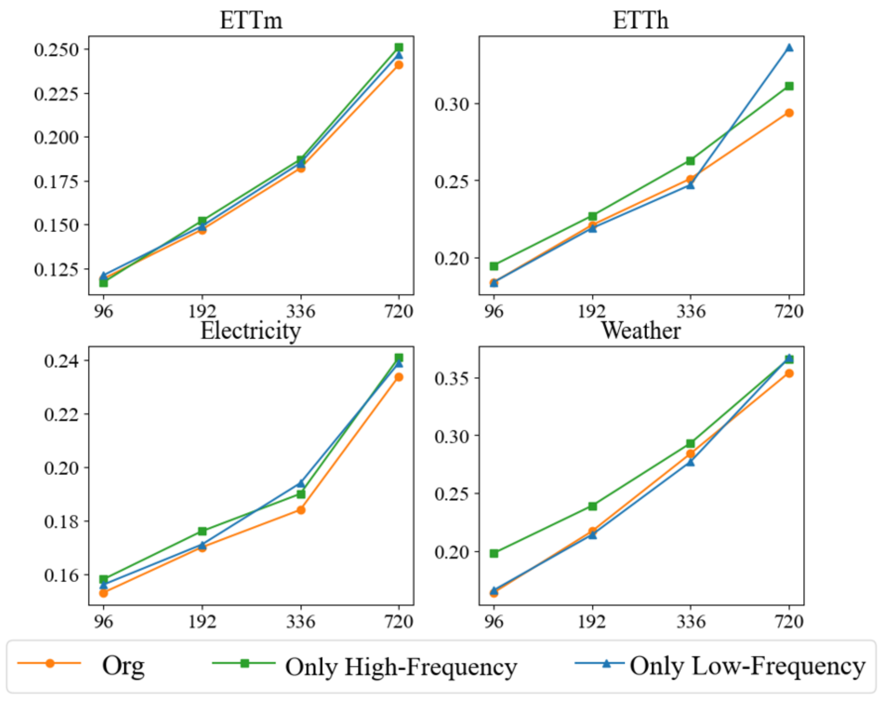
4.3. Ablation Studies

In order to comprehensively evaluate the performance of our proposed method in multivariate time-series forecasting, we conducted several ablation experiments using the mean square error (MSE) as the main evaluation metric. The purpose of the ablation experiments is to gain a deeper understanding of the contribution of each component in the model by systematically removing specific components and observing their impact on the model performance. This process helps to reveal the role of individual modules in capturing multivariate correlations and temporal patterns. Our ablation experiments are conducted on four different datasets to ensure that the performance of individual modules is reliably verified. We test three main configurations. The only low-frequency retains only the low-frequency trend processing module, which focuses on capturing long-term trends in multivariate time series through variable-oriented attention mechanisms and convolutional layers, while the high-frequency portion replaces the existing model with a simple linear layer. The Only High-Frequency retains the high-frequency fluctuations module, which focuses on capturing short-term fluctuations in a time series through multigranular modeling and time-step attention mechanisms, while the low frequency part replaces the existing model with a simple linear layer. Org integrates both the low and high frequency components to take advantage of their combined strengths for complete frequency and time-domain modeling of multivariate time series.

The experimental results, illustrated in Figure 3, demonstrate the superiority of the original method (Org) over its de-componentized versions across various prediction lengths, underscoring the importance of integrating both low- and high-frequency processing modules. Specifically, the original method excels in long-term forecasting, affirming the necessity of merging frequency and time domain information to effectively capture both long-term trends and short-term fluctuations. When only the low-frequency module is retained, the model adeptly captures long-term trends but struggles with short-term fluctuations. This configuration, while second-best in short-term forecasting, highlights the significance of long-term trends in predicting short-term changes. However, the absence of a high-frequency module limits its ability to address rapid short-term dynamics. Conversely, configurations retaining only the high-frequency module excel in short-term fluctuation management, performing comparably or even surpassing the original method in tasks with shorter prediction lengths. This underscores the importance of multi-granularity modeling and time-step attention mechanisms for capturing complex short-term dependencies. Nevertheless, the performance of high-frequency-only configurations deteriorates in long-term forecasting due to their inability to model long-term trends. The optimal configuration remains the original method, which adeptly handles both global and local temporal dynamics by merging low- and high-frequency processing. The low-frequency component models long-term stable trends, while the high-frequency component addresses local fluctuations, ensuring a comprehensive modeling of temporal patterns and multivariate dependencies. This integrated approach achieves the lowest MSE values across all datasets and forecast lengths, markedly outperforming other configurations.

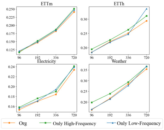
Figure 3. We evaluated the performance of our method in an ablation study using the mean squared error (MSE) metric for four prediction lengths 96, 192, 336, 720. By systematically removing specific components, we aimed to understand their contributions to learning multivariate correlations and series representations.

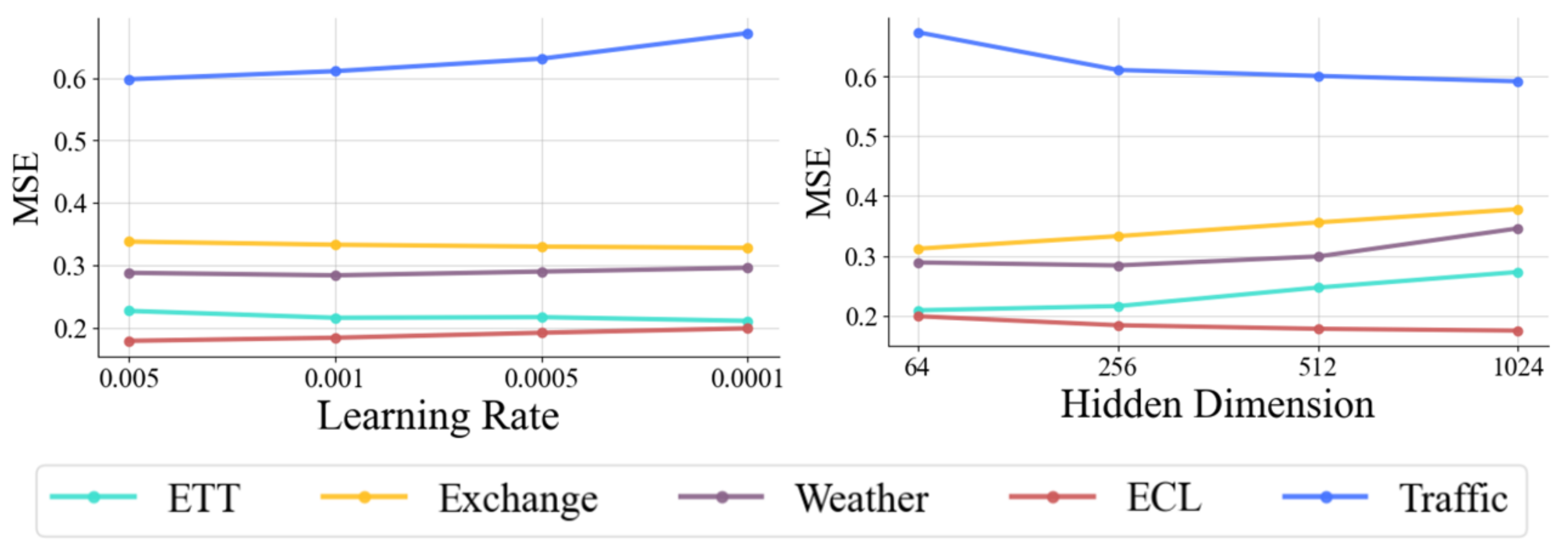
4.4. Hyperparameter Sensitivity

To deeply assess the sensitivity of our proposed method to key hyperparameters, we focus on analyzing two core parameters: learning rate and hidden dimension. Figure 4 illustrates the model’s performance in multivariate time-series forecasting with different parameter settings.

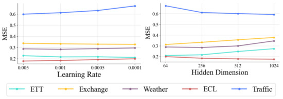
Figure 4. Hyperparameter sensitivity with respect to the learning rate and the hidden dimension of variate tokens. MSE is used as an evaluation metric, with lower representing better results. Different colored lines represent different datasets. x axis is the hyperparameter variation.

Learning rate is a key determinant of the dynamics of model training, which significantly affects the speed of convergence of gradient descent and the performance of the final model. Hidden dimension determines the model’s ability to represent and learn underlying patterns and complex dependencies in time-series data. The performance of the hyperparameters on different datasets reveals specific patterns, reflecting how the size of the dataset and the number of variables affect the choice of hyperparameters. On the ETT and Exchange datasets, each containing only seven variables, the datasets are small. For these datasets, the mean square error (MSE) decreases as the learning rate decreases, suggesting that the lower learning rate makes the model update more stable, which in turn improves performance. In addition, the MSE tends to increase as the hidden dimension increases, suggesting that too large a hidden dimension introduces unnecessary complexity and leads to model over-fitting, which in turn affects the prediction accuracy. In contrast, the opposite trend is observed on the larger datasets ECL (containing 321 variables) and Traffic (containing 862 variables). For these large-scale high-dimensional datasets, higher learning rates perform better, and the MSE increases as the learning rate decreases, suggesting that larger datasets require higher learning rates to effectively navigate the complex high-dimensional feature space. In addition, the MSE decreases significantly as the hidden dimension increases, indicating that a larger hidden dimension helps the model capture the complex patterns and multivariate dependencies in the dataset, which in turn improves the prediction performance.

These experimental results suggest that the hyperparameter settings of the model should be customized according to the size of the dataset and the number of variables. For small datasets with fewer variables, lower learning rates and smaller hidden dimensions help capture the underlying patterns and subtle dependencies in the time series, leading to better prediction performance. On the contrary, for large datasets with many variables, higher learning rates and larger hidden dimensions can better capture complex global patterns and avoid overfitting local features. Hyperparameter sensitivity analysis highlights the need to optimize hyperparameter settings for dataset characteristics. This flexible tuning is essential to improve model adaptation and provides a reliable guide for future model tuning. Future work will further optimize these hyperparameter settings and explore other key parameters, such as batch size and regularization coefficients, to further enhance the generalization ability and stability of the model in different time-series forecasting tasks.

4.5. Model Analysis

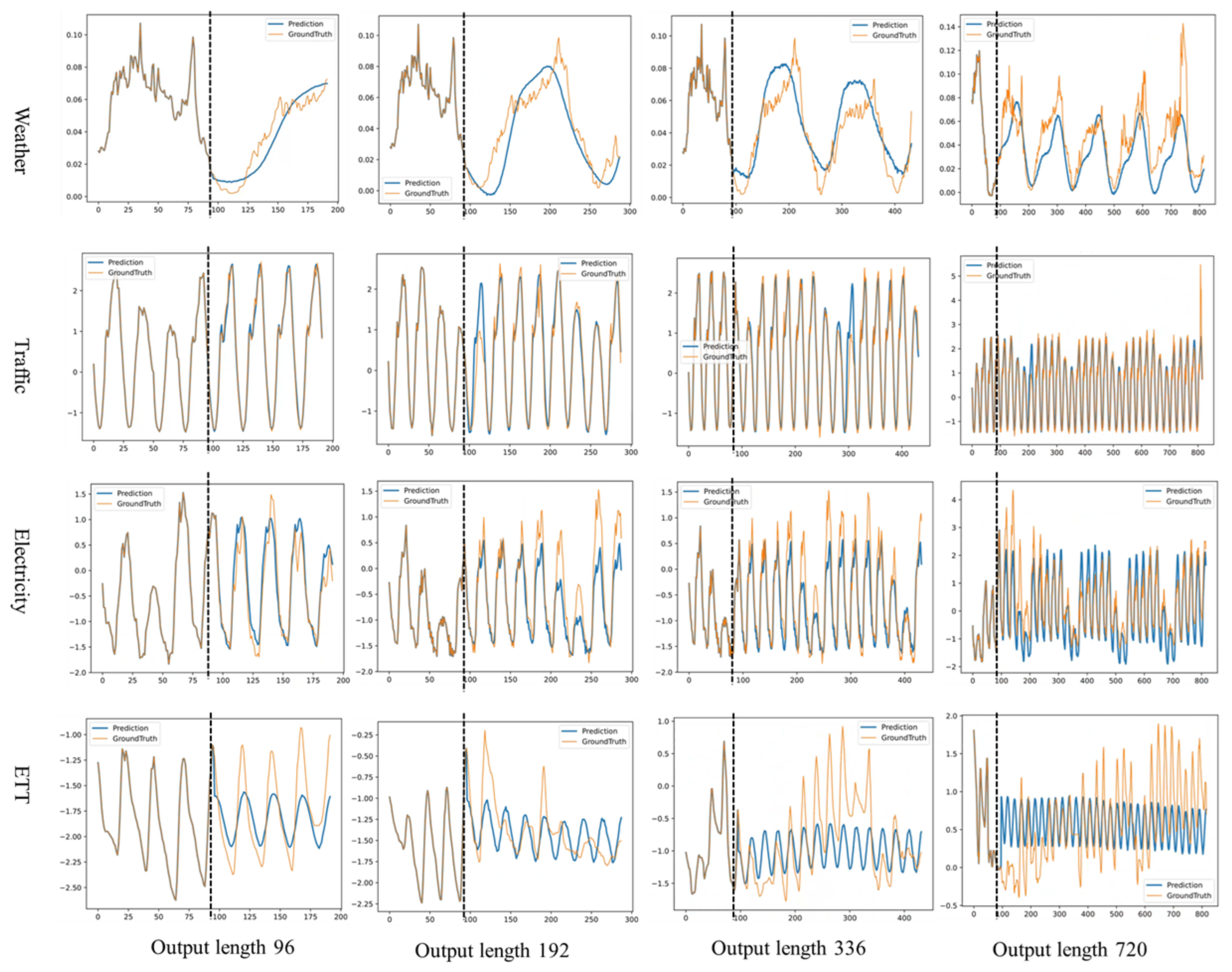
In order to comprehensively assess the predictive performance of our proposed model, we visualize the results for multiple datasets with different prediction lengths. This visualization approach provides us with a clear view to evaluate the performance of the model in multiple scenarios. The visualization results are shown in Figure 5.

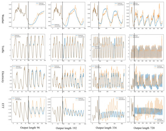
Figure 5. Example time-series forecasts are shown for the four datasets under the Prediction-96 to Prediction-720 settings. Orange lines are ground truth and blue lines are model predictions. In each of the example plots, the left side of the vertical dashed line shows the known input values and the right side shows the unknown predictions.

The model exhibits strong predictive capabilities across various datasets and forecast lengths. In the Weather dataset, it consistently and robustly captures the underlying trends at forecast lengths of 96 and 192, and maintained effective prediction over longer spans (336 and 720), showcasing its stability in managing extended periods of fluctuation. This success in long-term forecasting underscores the model’s adeptness at navigating complex trends and periodicities in time-series data. In the Traffic dataset, the model excels across all forecast settings, accurately identifying both trend and cyclical patterns, including the upper and lower bounds of traffic cycles and recurring traffic flow patterns. However, it occasionally faltered in capturing anomalous fluctuations at the longest forecast length of 720, highlighting its limitations with extreme variations and outliers. For the Electricity dataset, the model captures general trends and volatilities well, but displayed a conservative tendency in estimating the extreme ranges of values, particularly over longer time spans. This conservative bias, likely due to a preference for fitting smoother time-series patterns during training, restricted its adaptability to highly fluctuating data. Similarly, in the ETT dataset, the model’s predictions are conservative, constrained by the smoothness and distributional biases of the data. While it effectively captures periodic fluctuations, it struggled with extreme value predictions. The gradient descent training method, although effective for smooth trends, showed limitations with highly variable or extreme data points. Despite these challenges, the model’s robust handling of regular fluctuations and horizontal trends ensures its reliability in the short- to medium-term forecasting, affirming its utility across diverse forecasting scenarios.

5. Conclusions

In this paper, we propose a novel multivariate time-series forecasting model that integrates both frequency-domain and time-domain decomposition to address the limitations of traditional time-domain-only approaches. By decomposing the input series into low-frequency stable components and high-frequency fluctuation components, our model effectively captures the intricate dynamics of time-series data. The low-frequency component is modeled using Fourier-enhanced techniques and variable-wise attention mechanisms, enabling the extraction of long-term multivariate trends. Simultaneously, the high-frequency component leverages multi-granularity temporal modeling to capture short-term variations across multiple time scales, ensuring a comprehensive representation of time-series dynamics. Extensive experiments on multiple benchmark datasets demonstrate that our model consistently outperforms state-of-the-art methods in both short-term and long-term forecasting tasks. The results highlight the model’s ability to achieve superior accuracy and robustness across diverse scenarios, validating the effectiveness of its dual-domain decomposition and specialized pipelines for stable and fluctuating components.

In future work, we aim to further enhance the model’s scalability and applicability to more complex and higher-dimensional datasets. By incorporating advanced time-series analysis techniques and exploring novel architectures, we plan to improve the model’s adaptability for real-time forecasting, anomaly detection, and other practical applications. Additionally, we will investigate the integration of domain-specific knowledge to tailor the framework for specific industries, such as finance, healthcare, and energy.

References

- He, Z.; Li, C.; Shen, Y.; He, A. A hybrid model equipped with the minimum cycle decomposition concept for short-term forecasting of electrical load time series. Neural Process. Lett. 2017, 46, 1059–1081. [Google Scholar] [CrossRef]
- Hu, W.; Yan, L.; Liu, K.; Wang, H. A short-term traffic flow forecasting method based on the hybrid PSO-SVR. Neural Process. Lett. 2016, 43, 155–172. [Google Scholar] [CrossRef]
- Gundu, V.; Simon, S.P. Short term solar power and temperature forecast using recurrent neural networks. Neural Process. Lett. 2021, 53, 4407–4418. [Google Scholar] [CrossRef]
- Alyousifi, Y.; Othman, M.; Sokkalingam, R.; Faye, I.; Silva, P.C. Predicting daily air pollution index based on fuzzy time series markov chain model. Symmetry 2020, 12, 293. [Google Scholar] [CrossRef]
- Namasudra, S.; Dhamodharavadhani, S.; Rathipriya, R. Nonlinear neural network based forecasting model for predicting COVID-19 cases. Neural Process. Lett. 2023, 55, 171–191. [Google Scholar] [CrossRef]
- Yasar, H.; Kilimci, Z.H. US dollar/Turkish lira exchange rate forecasting model based on deep learning methodologies and time series analysis. Symmetry 2020, 12, 1553. [Google Scholar] [CrossRef]
- Kirisci, M.; Cagcag Yolcu, O. A new CNN-based model for financial time series: TAIEX and FTSE stocks forecasting. Neural Process. Lett. 2022, 54, 3357–3374. [Google Scholar] [CrossRef]
- Cruz-Nájera, M.A.; Treviño-Berrones, M.G.; Ponce-Flores, M.P.; Terán-Villanueva, J.D.; Castán-Rocha, J.A.; Ibarra-Martínez, S.; Santiago, A.; Laria-Menchaca, J. Short time series forecasting: Recommended methods and techniques. Symmetry 2022, 14, 1231. [Google Scholar] [CrossRef]
- Wang, C.; Zhang, Z.; Wang, X.; Liu, M.; Chen, L.; Pi, J. Frequency-Enhanced Transformer with Symmetry-Based Lightweight Multi-Representation for Multivariate Time Series Forecasting. Symmetry 2024, 16, 797. [Google Scholar] [CrossRef]
- Parmezan, A.R.S.; Souza, V.M.; Batista, G.E. Evaluation of statistical and machine learning models for time series prediction: Identifying the state-of-the-art and the best conditions for the use of each model. Inf. Sci. 2019, 484, 302–337. [Google Scholar] [CrossRef]
- Bontempi, G.; Ben Taieb, S.; Le Borgne, Y.A. Machine learning strategies for time series forecasting. In Business Intelligence: Second European Summer School, eBISS 2012, Brussels, Belgium, July 15–21, 2012, Tutorial Lectures 2; Springer: Berlin/Heidelberg, Germany, 2013; pp. 62–77. [Google Scholar]
- Sapankevych, N.I.; Sankar, R. Time series prediction using support vector machines: A survey. IEEE Comput. Intell. Mag. 2009, 4, 24–38. [Google Scholar] [CrossRef]
- Masini, R.P.; Medeiros, M.C.; Mendes, E.F. Machine learning advances for time series forecasting. J. Econ. Surv. 2023, 37, 76–111. [Google Scholar] [CrossRef]
- Lai, G.; Chang, W.C.; Yang, Y.; Liu, H. Modeling long-and short-term temporal patterns with deep neural networks. In Proceedings of the 41st International ACM SIGIR Conference on Research & Development in Information Retrieval, Ann Arbor, MI, USA, 8–12 July 2018; pp. 95–104. [Google Scholar]
- Oreshkin, B.N.; Carpov, D.; Chapados, N.; Bengio, Y. NBEATS: Neural basis expansion analysis for interpretable time series forecasting. arXiv 2019, arXiv:1905.10437. [Google Scholar]
- Lim, B.; Zohren, S. Time-series forecasting with deep learning: A survey. Philos. Trans. R. Soc. A 2021, 379, 20200209. [Google Scholar] [CrossRef]
- Han, Z.; Zhao, J.; Leung, H.; Ma, K.F.; Wang, W. A review of deep learning models for time series prediction. IEEE Sens. J. 2019, 21, 7833–7848. [Google Scholar] [CrossRef]
- Salinas, D.; Flunkert, V.; Gasthaus, J.; Januschowski, T. DeepAR: Probabilistic forecasting with autoregressive recurrent networks. Int. J. Forecast. 2020, 36, 1181–1191. [Google Scholar] [CrossRef]
- Qin, Y.; Song, D.; Chen, H.; Cheng, W.; Jiang, G.; Cottrell, G. A dual-stage attention-based recurrent neural network for time series prediction. arXiv 2017, arXiv:1704.0297. [Google Scholar]
- Borovykh, A.; Bohte, S.; Oosterlee, C.W. Conditional time series forecasting with convolutional neural networks. arXiv 2017, arXiv:1703.04691. [Google Scholar]
- Sen, R.; Yu, H.F.; Dhillon, I.S. Think globally, act locally: A deep neural network approach to high-dimensional time series forecasting. Adv. Neural Inf. Process. Syst. 2019, 32, 4837–4846. [Google Scholar]
- Bai, S.; Kolter, J.Z.; Koltun, V. An empirical evaluation of generic convolutional and recurrent networks for sequence modeling. arXiv 2018, arXiv:1803.01271. [Google Scholar]
- Vaswani, A.; Shazeer, N.; Parmar, N.; Uszkoreit, J.; Jones, L.; Gomez, A.N.; Kaiser, Ł.; Polosukhin, I. Attention is all you need. Adv. Neural Inf. Process. Syst. 2017, 30, 6000–6010. [Google Scholar]
- Zhou, H.; Zhang, S.; Peng, J.; Zhang, S.; Li, J.; Xiong, H.; Zhang, W. Informer: Beyond efficient transformer for long sequence time-series forecasting. Proc. AAAI Conf. Artif. Intell. 2021, 35, 11106–11115. [Google Scholar] [CrossRef]
- Koopmans, L.H. The Spectral Analysis of Time Series; Elsevier: Amsterdam, The Netherlands, 1995. [Google Scholar]
- Beran, J. Statistics for Long-Memory Processes; Routledge: London, UK, 2017. [Google Scholar]
- Wu, H.; Xu, J.; Wang, J.; Long, M. Autoformer: Decomposition transformers with auto-correlation for long-term series forecasting. Adv. Neural Inf. Process. Syst. 2021, 34, 22419–22430. [Google Scholar]
- Zhou, T.; Ma, Z.; Wen, Q.; Wang, X.; Sun, L.; Jin, R. Fedformer: Frequency enhanced decomposed transformer for long-term series forecasting. In Proceedings of the International Conference on Machine Learning, PMLR, Baltimore, MD, USA, 17–23 July 2022; pp. 27268–27286. [Google Scholar]
- Xu, Z.; Zeng, A.; Xu, Q. FITS: Modeling time series with 10k parameters. arXiv 2023, arXiv:2307.03756. [Google Scholar]
- Wu, H.; Hu, T.; Liu, Y.; Zhou, H.; Wang, J.; Long, M. Timesnet: Temporal 2d-variation modeling for general time series analysis. arXiv 2022, arXiv:2210.02186. [Google Scholar]
- Lee-Thorp, J.; Ainslie, J.; Eckstein, I.; Ontanon, S. Fnet: Mixing tokens with fourier transforms. arXiv 2021, arXiv:2105.03824. [Google Scholar]
- Zhou, T.; Ma, Z.; Wang, X.; Wen, Q.; Sun, L.; Yao, T.; Yin, W.; Jin, R. Film: Frequency improved legendre memory model for long-term time series forecasting. Adv. Neural Inf. Process. Syst. 2022, 35, 12677–12690. [Google Scholar]
- Li, S.; Jin, X.; Xuan, Y.; Zhou, X.; Chen, W.; Wang, Y.X.; Yan, X. Enhancing the locality and breaking the memory bottleneck of transformer on time series forecasting. In Proceedings of the 33rd Conference on Neural Information Processing Systems (NeurIPS 2019), Vancouver, BC, Canada, 8–14 December 2019. [Google Scholar]
- Liu, S.; Yu, H.; Liao, C.; Li, J.; Lin, W.; Liu, A.X.; Dustdar, S. Pyraformer: Low-complexity pyramidal attention for long-range time series modeling and forecasting. In Proceedings of the International Conference on Learning Representations, Vienna, Austria, 4 May 2021. [Google Scholar]
- Liu, Y.; Hu, T.; Zhang, H.; Wu, H.; Wang, S.; Ma, L.; Long, M. itransformer: Inverted transformers are effective for time series forecasting. arXiv 2023, arXiv:2310.06625. [Google Scholar]
- Dosovitskiy, A. An image is worth 16x16 words: Transformers for image recognition at scale. arXiv 2020, arXiv:2010.11929. [Google Scholar]
- Wan, J.; Xia, N.; Yin, Y.; Pan, X.; Hu, J.; Yi, J. TCDformer: A transformer framework for non-stationary time series forecasting based on trend and change-point detection. Neural Netw. 2024, 173, 106196. [Google Scholar] [CrossRef]
- Wang, Y.; Wu, H.; Dong, J.; Liu, Y.; Qiu, Y.; Zhang, H.; Wang, J.; Long, M. Timexer: Empowering transformers for time series forecasting with exogenous variables. arXiv 2024, arXiv:2402.19072. [Google Scholar]
- Nelson, B.K. Time series analysis using autoregressive integrated moving average (ARIMA) models. Acad. Emerg. Med. 1998, 5, 739–744. [Google Scholar] [CrossRef]
- Sowell, F. Modeling long-run behavior with the fractional ARIMA model. J. Monet. Econ. 1992, 29, 277–302. [Google Scholar] [CrossRef]
- Zeng, A.; Chen, M.; Zhang, L.; Xu, Q. Are transformers effective for time series forecasting? Proc. AAAI Conf. Artif. Intell. 2023, 37, 11121–11128. [Google Scholar] [CrossRef]
- Kalekar, P.S. Time Series Forecasting Using Holt-Winters Exponential Smoothing. Kanwal Rekhi School of Information Technology, Mumbai, India. 2004, pp. 1–13. Available online: https://c.mql5.com/forextsd/forum/69/exponentialsmoothing.pdf (accessed on 3 April 2025).
- Hochreiter, S.; Schmidhuber, J. Long short-term memory. Neural Comput. 1997, 9, 1735–1780. [Google Scholar] [CrossRef]
- Wang, H.; Peng, J.; Huang, F.; Wang, J.; Chen, J.; Xiao, Y. Micn: Multi-scale local and global context modeling for long-term series forecasting. In Proceedings of the Eleventh International Conference on Learning Representations, Virtual, 25–29 April 2022. [Google Scholar]
- Guo, Y.; Guo, J.; Sun, B.; Bai, J.; Chen, Y. A new decomposition ensemble model for stock price forecasting based on system clustering and particle swarm optimization. Appl. Soft Comput. 2022, 130, 109726. [Google Scholar] [CrossRef]
- Li, Y.; Liu, J.; Teng, Y. A decomposition-based memetic neural architecture search algorithm for univariate time series forecasting. Appl. Soft Comput. 2022, 130, 109714. [Google Scholar] [CrossRef]
- Zhang, F.; Guo, T.; Wang, H. DFNet: Decomposition fusion model for long sequence time-series forecasting. Knowl. Based Syst. 2023, 277, 110794. [Google Scholar] [CrossRef]
- Russakovsky, O.; Deng, J.; Su, H.; Krause, J.; Satheesh, S.; Ma, S.; Huang, Z.; Karpathy, A.; Khosla, A.; Bernstein, M.; et al. ImageNet large scale visual recognition challenge. Int. J. Comput. Vis. 2015, 115, 211–252. [Google Scholar] [CrossRef]
- Ba, J.L.; Kiros, J.R.; Hinton, G.E. Layer normalization. arXiv 2016, arXiv:1607.06450. [Google Scholar]
- Ulyanov, D.; Vedaldi, A.; Lempitsky, V. Instance normalization: The missing ingredient for fast stylization. In Proceedings of the Computer Vision–ECCV 2018: 15th European Conference, Munich, Germany, 8–14 September 2018; Part XIII. Springer: Berlin/Heidelberg, Germany, 2018; Volume 11217, p. 17. [Google Scholar]
- Gehring, J.; Auli, M.; Grangier, D.; Dauphin, Y.N. A convolutional encoder model for neural machine translation. arXiv 2016, arXiv:1611.02344. [Google Scholar]
- Van Den Oord, A.; Dieleman, S.; Zen, H.; Simonyan, K.; Vinyals, O.; Graves, A.; Kalchbrenner, N.; Senior, A.; Kavukcuoglu, K. Wavenet: A generative model for raw audio. arXiv 2016, arXiv:1609.03499. [Google Scholar]
- Paszke, A.; Gross, S.; Massa, F.; Lerer, A.; Bradbury, J.; Chanan, G.; Killeen, T.; Lin, Z.; Gimelshein, N.; Antiga, L.; et al. An imperative style, high-performance deep learning library. Adv. Neural Inf. Process. Syst. 1912, 32, 8026. [Google Scholar]
- Kingma, D.P.; Ba, J. A method for stochastic optimization. In Proceedings of the International Conference on Learning Representations (ICLR), San Diego, CA, USA, 7–9 May 2015; Volume 5, p. 6. [Google Scholar]
- Garza, A.; Mergenthaler-Canseco, M. TimeGPT-1. arXiv 2023, arXiv:2310.03589. [Google Scholar] [CrossRef]
Disclaimer/Publisher’s Note: The statements, opinions and data contained in all publications are solely those of the individual author(s) and contributor(s) and not of MDPI and/or the editor(s). MDPI and/or the editor(s) disclaim responsibility for any injury to people or property resulting from any ideas, methods, instructions or products referred to in the content. |
© 2025 by the authors. Licensee MDPI, Basel, Switzerland. This article is an open access article distributed under the terms and conditions of the Creative Commons Attribution (CC BY) license (https://creativecommons.org/licenses/by/4.0/).