Structural Damage Identification Using Data Fusion and Optimization of the Self-Adaptive Differential Evolution Algorithm

Abstract

This paper addresses the critical challenges of inadequate localization and low quantification precision in structural damage identification by introducing a novel approach that integrates Dempster–Shafer (D-S) evidence theory with the Self-Adaptive Differential Evolution (SDE) algorithm. First, modal parameters are extracted from a simply supported beam using the finite element (FE) method, and the corresponding index values are computed based on the formulated damage identification index equations. Next, these indices are applied to analyze damage localization in both single-position and multi-position scenarios within the simply supported beam. The SDE algorithm is then employed to dynamically optimize the initial weights and thresholds of various algorithms, ensuring the assignment of optimal values. Finally, the resulting data are input into the model for training, yielding a prediction model with enhanced accuracy that can precisely estimate the damage severity of the simply supported beam. The findings demonstrate that the three proposed damage identification indices—DI_1,i,j, DI_2,i,j, and DSDI_i,j—not only achieve high accuracy in damage localization but also significantly improve the precision of algorithms optimized by the SDE. These methods exhibit strong accuracy and robustness, providing a valuable reference for damage identification in small-to-medium-span simply supported beam bridges.

1. Introduction

Inevitably, various factors can significantly impact small and medium-span simply supported bridges. These factors include natural environmental erosion, traffic load effects, and material aging during continuous service, all of which gradually lead to varying levels of damage. The damage is typically distributed across different locations of the bridge and can range in severity and form, from minor cracks to severe structural deformations. However, traditional bridge inspection methods face significant challenges, including limited accuracy, insufficient global and real-time capabilities, and substantial human subjectivity, which often lead to delayed damage detection. If not addressed in a timely manner, undetected damage can pose serious risks to the safety and functionality of the bridge. Therefore, research on accurate damage identification for small and medium-span simply supported beam bridges holds considerable practical importance.

Among the existing damage identification methods, those based on dynamic fingerprints are the most widely used. These methods include those that utilize natural frequencies, flexibility matrices, modal strain energy, and curvature modes, among others [1,2,3,4]. Among these, methods based on curvature mode indicators have garnered significant attention from both domestic and international scholars. Since the proposal of the curvature mode-based structural damage identification method by Pandey A.K. et al. [5] in 1991, its effectiveness and practicality have been widely promoted and applied. Although Ren X. et al. [6] introduced a wavelet difference indicator based on curvature modes, which improves sensitivity to small structural damages, curvature mode-based indicators still face issues such as large errors near displacement mode inflection points and reduced stability in higher-order curvature modes. These higher-order modes, although more sensitive to small damages, offer lower stability in damage identification.

To address these challenges and ensure comprehensive and accurate judgments, many researchers have introduced data fusion techniques to develop novel approaches for structural damage identification. For example, Huang T. et al. [7] proposed a structural damage identification method based on convolutional neural networks (CNNs) and data fusion to overcome the low accuracy in damage identification for complex frame structures. Jaramillo V.H. et al. [8] proposed a two-stage Bayesian inference data fusion method for structural damage identification to address the difficulty of diagnosing the health status of components in rotating machinery. Despite these advances, data fusion still faces limitations in quantifying damage levels.

In recent years, artificial intelligence (AI) algorithms have been widely adopted for the quantitative prediction of structural damage. For instance, Sadeghi F. et al. [9] proposed a damage quantification method by combining modal strain energy change ratios (MSECRs) with a general regression neural network (GRNN). Addressing the challenge of limited data availability, Li M. et al. [10] proposed a damage identification method using strain mode differences as input for CNNs. To enhance algorithm iteration speed and accuracy in structural damage quantification, Miao B. et al. [11] proposed a method using multi-scale wavelet coefficient modulus maxima as input for BP neural networks. To improve structural damage detection accuracy from sensor-collected data, Ghiasi R. et al. [12] proposed an optimized method using a social harmony search algorithm for the parameters of the least squares support vector machine and thin-plate spline wavelet kernels. Yan B. et al. [13] proposed a combined structural damage identification method based on support vector machines (SVMs) and BP neural networks to address the challenge of manually detecting early cracks in offshore platform support beams.

While the aforementioned algorithms have shown strong performance in structural damage quantification, BP and SVM algorithms still face challenges such as local optima, low diagnostic accuracy, and slow convergence in structural damage analysis. Although D-S evidence theory has been preliminarily applied to structural damage identification, extant methodologies exhibit two shortcomings: (1) Current D-S evidence theory implementations treat modal features as equally reliable inputs, overlooking their potential for conflict, which leads to an increase in error rates; and (2) many studies use D-S evidence theory as a post-processing fusion layer, lacking bidirectional interaction with upstream AI models, resulting in suboptimal noise immunity. To overcome the limitations of curvature modes, D-S evidence theory, BP, and SVM algorithms, this paper introduces three structural damage identification indicators (DI_1,i,j, DI_2,i,j, and data fusion indicator DSDI_i,j) based on curvature modes and D-S evidence theory. Additionally, the SDE-optimized BP and Support Vector Regression (SVR) algorithms are applied. Finally, the method is validated through numerical and experimental examples involving simply supported beams, demonstrating its effectiveness in location identification, damage quantification, and noise resistance under various damage conditions.

2. Basic Concepts and Definition of Damage Indicators

2.1. Curvature Modal

According to the theory of material mechanics, the curvature function at any point on a beam’s cross-section is given by the following:

$$Q\left(x,y\right)={\displaystyle \frac{{\mathsf{\partial }}^2{\varphi }_j\left(x\right)}{\mathsf{\partial }{x}^2}}={\displaystyle \frac{M_x}{EI\left(x\right)}}$$

(1)

where Q(x,y) denote the curvature function at a point with coordinates (x,y) at a specific instant, and let M_x represent the bending moment at point x.

By combining Equation (1) and the small deflection theory, the structural curvature function can be rewritten as follows:

$$Q(x,y)={\displaystyle \frac{M_x}{EI(x)}}={\displaystyle \sum _{i=1}^{\infty }{\varphi }_j^{″}(x)q_i(t)}$$

(2)

where q_i(t) refers to the modal coordinate as a function of time t, and ${\varphi }_j^{″}\left(x\right)$ denotes a specific curvature mode of the structure at point x.

From Equations (1) and (2), it can be observed that the curvature modes change with variations in the beam’s stiffness and are highly sensitive to structural damage. Additionally, there is a one-to-one correspondence between curvature modes and displacement modes [14].

2.2. Definition of Damage Indicators

Due to the absence of sensors capable of directly measuring the structural curvature response and the relative ease of obtaining displacement modes, the central difference method is employed to indirectly calculate the curvature modes before and after structural damage. The expression is as follows:

$${\varphi }_{i,j,d}^{″}={\displaystyle \frac{{\varphi }_{i,j-1,d}-2{\varphi }_{i,j,d}+{\varphi }_{i,j+1,d}}{l^2}}$$

(3)

$${\varphi }_{i,j,u}^{″}={\displaystyle \frac{{\varphi }_{i,j-1,u}-2{\varphi }_{i,j,u}+{\varphi }_{i,j+1,u}}{l^2}}$$

(4)

where ${\varphi }_{\mathrm{i},j,d}^{″}$ represents the i-th curvature mode at point j when the structure is damaged, ${\varphi }_{i,j,u}^{″}$ represents the i-th curvature mode at point j when the structure is undamaged, ϕ_i,j,d represents the i-th displacement mode at point j when the structure is damaged, ϕ_i,j,u represents the i-th displacement mode at point j when the structure is undamaged, j denotes the structural node number, and n represents the total number of structural nodes.

To avoid cancelation of the positive and negative curvature modes at each node during summation, the absolute values of the curvature modes at each node are taken. The weights of the modal curvature at the j-th node before and after damage, in the i-th mode, in the overall structural modal curvature, are given by Equations (5) and (6), respectively. The expression is as follows:

$$F_{i,j,d}={\displaystyle \frac{\left|{\varphi }_{i,j,d}^{″}\right|}{{\displaystyle \sum _{j=1}^n\left|{\varphi }_{i,j,d}^{″}\right|}}}$$

(5)

$$F_{i,j,u}={\displaystyle \frac{\left|{\varphi }_{i,j,u}^{″}\right|}{{\displaystyle \sum _{j=1}^n\left|{\varphi }_{i,j,u}^{″}\right|}}}$$

(6)

where ${\displaystyle \sum _{j=1}^n\left|{\varphi }_{i,j,d}^{″}\right|}$ represents the sum of the absolute values of the i-th curvature mode at point j when the structure is damaged, and ${\displaystyle \sum _{j=1}^n\left|{\varphi }_{i,j,u}^{″}\right|}$ represents the sum of the absolute values of the i-th curvature mode at point j of the structure in its undamaged state.

Therefore, the sum of the overall structural damage index F_i,j,d and the undamaged index F_i,j,u equals 1, as expressed by the following:

$$E_{i,j,d}={\displaystyle \sum _{j=1}^n{F}_{i,j,d}}=1$$

(7)

$$E_{i,j,u}={\displaystyle \sum _{j=1}^n{F}_{i,j,u}}=1$$

(8)

Dividing Equation (5) by Equation (6) results in Equation (9), where the value is less than or equal to 1 when the structural element is undamaged and greater than 1 when the structural element is damaged.

$${\phi }_{1,i,j}={\displaystyle \frac{F_{i,j,d}}{F_{i,j,u}}}$$

(9)

The strain energy U for a one-dimensional Euler–Bernoulli beam structure can be expressed as U. If the beam is divided into n equal segments, the strain energy in the m-th segment is expressed as U_m, with the following expression:

$$U={\displaystyle \frac{1}{2}}{\displaystyle \sum _{i=1}^n{(EI)}_i}{({\varphi }_i^{"})}^2$$

(10)

$$U_m={\displaystyle \frac{1}{2}}{(EI)}_m{({\varphi }_m^{"})}^2$$

(11)

Based on the assumptions of Euler–Bernoulli beam theory, including no torsion and small deflection assumptions, the bending stiffness EI of the beam’s cross-section is approximately constant along the length of the beam, thus,

$$F_{m,u}={\displaystyle \frac{U_{m,u}}{U}}={\displaystyle \frac{{({\varphi }_{m,u}^{"})}^2}{{\displaystyle \sum _{i=1}^n{({\varphi }_{m,u}^{"})}^2}}}$$

(12)

$$F_{m,d}={\displaystyle \frac{U_{m,d}}{U}}={\displaystyle \frac{{({\varphi }_{m,d}^{"})}^2}{{\displaystyle \sum _{i=1}^n{({\varphi }_{m,d}^{"})}^2}}}$$

(13)

Dividing Equation (13) by Equation (12) results in Equation (14), as expressed by

$${\phi }_{2,i,j}={\displaystyle \frac{F_{m,d}}{F_{m,u}}}$$

(14)

When using the two indicators φ_1,i,j and φ_2,i,j to identify structural damage, certain limitations arise. First, significant errors may occur near the inflection points of the displacement mode. Second, high-order curvature modes exhibit lower stability in damage detection compared to low-order modes and are more sensitive to minor damages.

To address the first limitation, the frequency w_i,d during structural damage is introduced as a weighting factor. This frequency-based weighting mechanism assigns higher priority to low-order curvature modes and lower priority to high-order modes, reflecting their distinct sensitivities to damage. Low-order modes dominate structural vibration energy and exhibit greater stability in global damage detection, whereas high-order modes, while sensitive to localized damage, are prone to noise amplification and numerical instability. The expression is the following:

$$U{I}_{1,i,j}={\displaystyle \frac{{\phi }_{1,i,j}}{w_{i,d}^2}}$$

(15)

$$U{I}_{2,i,j}={\displaystyle \frac{{\phi }_{2,i,j}}{w_{i,d}^2}}$$

(16)

Let w_i,d denote the frequency of the i-th mode of the structure when damaged, where i represents the 1st, 2nd, and 3rd modes.

To address the second limitation, multiple modes (specifically, the first three modes) are incorporated to enhance the indicators, thereby improving damage detection performance. The expression is as follows:

$$F{I}_{1,i,j}={\displaystyle \sum _{i=1}^{n}U{I}_{1,i,j}}$$

(17)

$$F{I}_{2,i,j}={\displaystyle \sum _{i=1}^{n}U{I}_{2,i,j}}$$

(18)

Due to the lack of comparability between the indices derived from the above formulas, normalization is applied to the data obtained from Equations (17) and (18) to express each data point as a ratio relative to the total sum. The summation normalization method is selected for this purpose [15]. Consequently, the expressions for the first two damage identification indices (damage index, DI) are provided as follows:

$$D{I}_{1,i,j}={\displaystyle \frac{F{I}_{1,i,j}}{{\displaystyle \sum _{j=1}^{n}F{I}_{1,i,j}}}}$$

(19)

$$D{I}_{2,i,j}={\displaystyle \frac{F{I}_{2,i,j}}{{\displaystyle \sum _{j=1}^{n}F{I}_{2,i,j}}}}$$

(20)

The Dempster–Shafer (D-S) evidence theory, introduced in the 1960s, is a method used to express and synthesize uncertain information for decision-level information fusion [16,17]. Let m_j(A_i) represent the basic probability distribution function used to determine the damage of the i-th element based on the j-th damage index. The D-S evidence matrix fusion rule is given by the following:

$$D(A)=\left\{\begin{array}{cc}{\displaystyle \frac{{\displaystyle \sum _{\cap A_i=A}\prod _{1\le j\le n}{m}_j(A_i)}}{1-K}}& A\ne \varnothing \\ 0& A=\varnothing \end{array}\right.$$

(21)

In the equation, $K={\displaystyle \sum _{\cap A_i=\varnothing }{\displaystyle \prod _{1\le j\le n}{m}_j(A_i)}}$.

To enhance the accuracy of structural damage identification, data fusion is integrated with damage identification indices, resulting in the proposed damage identification index DSDI_i,j based on D-S evidence theory. The steps involved in the D-S evidence fusion method are illustrated in Figure 1.

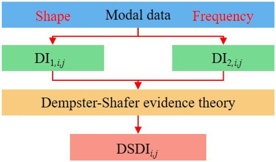
Figure 1. Dempster–Shafer evidence fusion method.

2.3. Optimizing the BP and SVR Using a Self-Adaptive Differential Evolution Algorithm

2.3.1. Backpropagation Neural Network

A BP neural network generally consists of an input layer, an output layer, and one or more hidden layers, and its expression is as follows:

$$y_j=\sigma \left({\displaystyle \sum _{i=1}^m{x}_i\times w_{i,j}+b_j}\right),\left(j=1,2,\cdots ,n\right)$$

(22)

$$z_k=\sigma \left({\displaystyle \sum _{i=1}^n{y}_j\times w_{j,k}+b_k}\right),\left(k=1,2,\cdots ,p\right)$$

(23)

where m, n, and p represent the number of neurons in the input layer, hidden layer, and output layer, respectively. σ denotes the activation function, N represents the number of training samples, x_i stands for the input value, y_j denotes the output value of the hidden layer, z_k is the output value, the weights are denoted as w_i,j and w_j,k, and the biases as b_j and b_k.

2.3.2. Support Vector Regression Method

Support vector machine (SVM), grounded in statistical theory, is primarily used to address binary and multi-class classification problems. Complementing SVM, Support Vector Regression (SVR) is employed to solve regression problems. Within the SVM and SVR frameworks, the selection of the kernel function is crucial, as it directly influences the model’s predictive performance and generalization ability. In this study, the Radial Basis Function (RBF) kernel is selected as the core kernel function, and its expression is given as follows:

$$K_{RBF}\left(x_i,x\right)=\exp \left(-\gamma {‖x_i-x‖}^2\right)$$

(24)

where γ is the kernel parameter, $\gamma ={\displaystyle \frac{1}{2{\sigma }^2}}$.

The kernel function in the original space is utilized to perform calculations in the high-dimensional feature space, which subsequently leads to the decision regression equation of the SVM.

$$y=f\left(x\right)={\displaystyle \sum _{i=1}^n\left({\alpha }_i^{*}-{\alpha }_i\right)}K\left(x_i,x\right)+\overline{b}$$

(25)

where $b_i=y_i-{\displaystyle \sum _{i=1}^n\left({\alpha }_i-{\alpha }_i^{*}\right)}K\left(x_i,x_j\right)\pm \epsilon , \overline{b}={\displaystyle \frac{1}{n}}{\displaystyle \sum _{i=1}^n{b}_i}$.

2.3.3. The Differential Evolution Algorithm

Differential Evolution (DE) is a heuristic optimization algorithm based on real-valued encoding and elitist principles. Initially introduced by Storn and Price in 1997, DE has evolved into one of the most widely used methods for solving complex optimization problems [18]. Compared to other algorithms, DE offers several advantages, including high optimization efficiency, fast convergence, fewer control variables, and robust performance [19]. The main components of the DE algorithm include mutation, crossover, and selection operations.

2.3.4. The SDE-BP and SDE-SVR Algorithms

In traditional Differential Evolution (DE) algorithms, the mutation factor controls the amplification ratio of the deviation vector. A mutation factor that is too large can negatively impact the global optimum, while a factor that is too small may reduce population diversity, leading to “premature convergence” [20]. In contrast to traditional methods, the SDE algorithm dynamically adjusts mutation factors to balance exploration and exploitation. Early iterations use larger mutation factors to enhance population diversity, reducing the risk of converging to local minima. Later iterations adopt smaller factors to refine solutions. To address these issues, this paper introduces an adaptive mutation factor. The adaptive mutation factor is determined by Equations (26) and (27) [21].

$$F=F_{\min }+\left(F_{\max }-F_{\min }\right)\times \lambda$$

(26)

$$\lambda =e^{1-{\displaystyle \frac{G_m}{G_m+1-G}}}$$

(27)

where F_min represents the minimum value of the mutation factor, F_max represents the maximum value of the mutation factor, G_m represents the maximum number of iterations, and G represents the current generation of evolution.

Therefore, this paper proposes a method for predicting structural damage severity based on SDE-optimized BP and SVR algorithms. The optimization process of the SDE algorithm for BP and SVR is illustrated in Figure 2 and Figure 3.

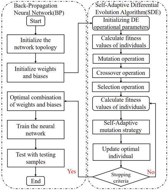
Figure 2. SDE-BP flowchart.

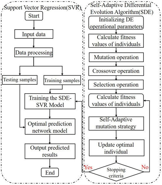
Figure 3. SDE-SVR flowchart.

3. Surrogate Model of a Simply Supported Beam

As illustrated in Figure 4, a rectangular-section simply supported beam is modeled using the finite element method (FEM) for numerical simulation analysis. The beam has a length of L = 20.00 m and section dimensions of b × h = 0.20 × 0.30 m². The material properties are as follows: Young’s modulus E = 210 GPa, Poisson’s ratio υ= 0.30, and density of ρ = 8000 kg/m³. Beam188 elements are employed, and the beam structure is discretized into 25 elements and 26 nodes with equal intervals of 0.8 m. Due to the challenges in extracting higher-order modes in practical engineering, this study focuses on the first three modes of the structure.

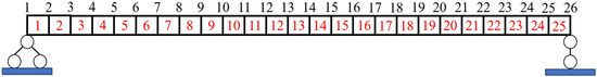
Figure 4. Finite element model of simply supported beam.

Damage to the beam is simulated by reducing the stiffness of selected elements. This study investigates beam damage under various scenarios, including single-location, two-location, and multi-location damage conditions. The specific damage scenarios are detailed in Table 1. Conditions 1–10 represent different levels of single damage, with damage levels of 5%, 10%, 15%, 20%, 25%, 30%, 35%, and 40%. Conditions 11–15 represent combinations of two damages with varying levels of 10%, 15%, 25%, 30%, 35%, and 40%. Conditions 16–20 represent combinations of multiple damages with levels of 10%, 15%, 20%, 25%, 30%, 35%, and 40%.

Table 1. The criteria for detecting damage in simply supported beams.

Damage Condition	Damage Element No.	Damage Index	Damage Degree (%)
1, 2, 3, 4, 5	5	DI1,i,j, DI2,i,j, DSDIi,j	10, 15, 20, 30, 40
6, 7, 8, 9, 10	9	DI1,i,j, DI2,i,j, DSDIi,j	5, 10, 25, 35, 40
11, 12	5–17	DI1,i,j, DI2,i,j, DSDIi,j	10–30, 40–40
13, 14, 15	13–17	DI1,i,j, DI2,i,j, DSDIi,j	15–15, 25–35, 30–30
16, 17	9–13–17	DI1,i,j, DI2,i,j, DSDIi,j	10–20–30, 15–25–35
18, 19, 20	9–13–21	DI1,i,j, DI2,i,j, DSDIi,j	15–15–15, 25–25–25, 40–40–40

Table 2 presents the first three modal frequencies for selected undamaged and damaged conditions. Figure 5 shows the first three mode shapes of the undamaged simply supported beam.

Table 2. Frequency of some cases.

	Frequency	1st-Order Frequency	2nd-Order Frequency	3rd-Order Frequency
Damage Condition
Non-DC		1.7468	7.0401	16.0408
DC1		1.7428	6.9855	15.8230
DC2		1.7415	6.9707	15.7840
DC3		1.7400	6.9543	15.7410
$⋮$		$⋮$	$⋮$	$⋮$

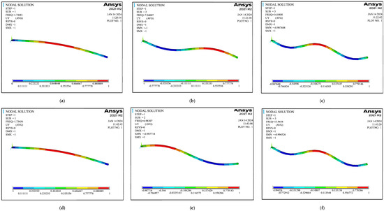
Figure 5. Modal shape cloud diagram. Non−damage case: (a) 1st order mode; (b) 2nd order mode; and (c) 3rd order mode. Damage case: (d) 1st order mode; (e) 2nd order mode; and (f) 3rd order mode.

4. Damage Identification of a Simply Supported Beam

4.1. Damage Localization of a Simply Supported Beam

Existing studies have demonstrated that data fusion, as an advanced technique for processing multi-source information, plays a crucial role in structural damage identification. Specifically, in damage diagnosis, integrating multiple local diagnostic results using D-S evidence theory enhances the credibility of true faults, reduces the credibility of false faults, decreases uncertainty, and improves diagnostic accuracy, thereby providing strong support for structural health monitoring [22]. Therefore, this section presents numerical simulations of a simply supported beam under various damage scenarios. The indicators DI_1,i,j, DI_2,i,j, and DSDI_i,j are then calculated for damage localization analysis, with the results shown in Figure 6, Figure 7, Figure 8 and Figure 9. In practical engineering applications, due to the greater contribution of low-order modes to structural vibration and the challenges in obtaining high-order modes, this study focuses on the first three modal data of the simply supported beam structure.

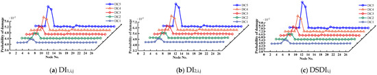
Figure 6. Damage identification under operating Conditions 1−5.

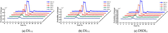
Figure 7. Damage identification under operating Conditions 6−10.

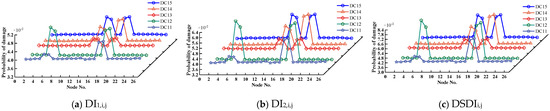
Figure 8. Damage identification under operating Conditions 11–15.

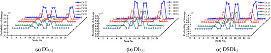
Figure 9. Damage identification under operating Conditions 16−20.

From Figure 6, Figure 7, Figure 8 and Figure 9, the following observations can be made:

(1)

Single Damage Scenarios: The indicators DI_1,i,j, DI_2,i,j, and DSDI_i,j accurately identify the damage location, with the peak value occurring at the damage site. As the damage increases, the severity also rises proportionally. All three indicators effectively reflect the severity of the damage qualitatively.

(2)

Comparing Damage Locations: When the same level of damage occurs at different locations, the peak values at each damage site are nearly identical. The DSDI_i,j indicator exhibits the largest peak, followed by DI_2,i,j, with DI_1,i,j showing the smallest peak. All indicators provide an initial assessment of the relative damage levels at the affected elements.

(3)

Multiple Damage Scenarios: In cases of multiple damage scenarios, when different elements undergo varying or identical levels of damage, the damage indicators remain unaffected by the different damage levels or units.

(4)

Comparison with Curvature Mode Indicators: When comparing the damage identification results, DI_1,i,j, DI_2,i,j, and DSDI_i,j all outperform the curvature mode indicators. They effectively address the large errors near displacement mode inflection points and the lower stability of higher-order curvature modes compared to lower-order modes, demonstrating superior performance in damage identification.

(5)

Integration Using D-S Evidence Theory: After integrating multi-source information with D-S evidence theory, the peak values of the damage locations are significantly enhanced, and interference from non-damaged locations is effectively suppressed. This integration substantially improves the accuracy of damage identification. It overcomes the limited sensitivity of the first two indicators in detecting minor damage and constructs the high-accuracy DSDI_i,j indicator, providing a more reliable reference for structural damage identification.

In conclusion, the structural damage identification indicators DI_1,i,j, DI_2,i,j, and DSDI_i,j can accurately locate damage within the structure. The latter indicator (DSDI_i,j) shows more pronounced peak values at damage sites compared to the former, and all three indicators can preliminarily assess the severity of damage at the affected nodes.

4.2. Influence of Measurement Noise

Structural damage identification in practical engineering is often influenced by various sources of noise, such as environmental factors and measurement errors. To align closely with real-world engineering scenarios, a noise robustness analysis is performed on the simply supported beam to assess the resilience of the proposed method. Given that noise levels in most engineering projects, particularly in controlled structural health monitoring systems, typically range between 1% and 2% due to sensor precision and environmental interference, this study examines noise robustness by adding 1% and 2% Gaussian white noise to the modal data [10,22]. Due to space limitations, this paper focuses on analyzing the two-position damage scenarios (Conditions 11–15) of the simply supported beam. The damage identification results under different noise levels are presented in Figure 10.

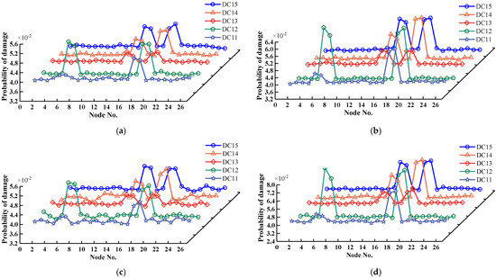
Figure 10. Noise damage identification of indicators for simple supported beam bridge under Conditions 11–15: (a) identification of indicator DI_1,i,j under 1% Noise Conditions 11–15 damage identification; (b) identification of indicator DI_2,i,j under 1% Noise Conditions 11–15 damage identification; (c) identification of indicator DI_1,i,j under 2% Noise Conditions 11–15 damage identification; and (d) identification of indicator DSDI_i,j under 2% Noise Conditions 11–15 damage identification.

From the results in Figure 10, the following observations can be made:

(1)

Noise Impact on Damage Indicators: As shown in Figure 8c and Figure 10a, after introducing noise to nodes 5 and 6 in Condition 11, the peak probabilities of the damage identification indicators (DI_1,i,j, DI_2,i,j, and DSDI_i,j) at the damage locations slightly decrease, while the peak probabilities at non-damaged locations increase. This suggests that noise negatively affects the performance of the indicators in damage recognition.

(2)

Comparison of Indicators’ Noise Robustness: As depicted in Figure 10a,b, for indicator DI_1,i,j, the peak values at nodes 5 and 6 in Condition 11 before noise introduction are 0.039805 and 0.039625, respectively. After adding 1% noise, these values decrease to 0.039284 and 0.039427, respectively. For indicator DI_2,i,j, under the same condition, the peak values before noise addition are 0.041058 and 0.040685, respectively, and, after adding noise, the values become 0.040687 and 0.040517. Therefore, the noise robustness of DI_2,i,j is stronger than that of DI_1,i,j, although both indicators exhibit consistent damage recognition performance.

(3)

Impact of D-S Data Fusion: As shown in Figure 10c,d, compared to before fusion, the DSDI_i,j indicator after D-S data fusion exhibits a higher peak probability at the damage location under the same damage and noise conditions, with less sensitivity to noise interference.

4.3. Damage Quantification of a Simply Supported Beam

From the above analysis, it can be seen that the damage identification indicators constructed in this paper can preliminarily determine the damage location and its severity, but it is difficult to accurately predict the exact level of damage at the corresponding locations. Regarding the prediction of damage severity, this paper proposes to optimize the damage identification methods of BP and SVR algorithms by introducing SDE.

A total of 36 × 25 data points are selected from the sample data as training data and 10 × 25 data points as test data. In the Matlab R2021b environment, models for BP, SVR, DE-BP, DE-SVR, SDE-BP, and SDE-SVR are established. The training data are input into each respective model, which learns the relationship between the peak values of the damaged elements and their corresponding damage degrees. The models for BP, SVR, DE-BP, DE-SVR, SDE-BP, and SDE-SVR are trained to develop predictive models. The three indicators, DI_1,i,j, DI_2,i,j, and DSDI_i,j, are validated for their quantitative performance in identifying single-point, two-point, and multi-point damage in simply supported beams across different algorithms. The training and test sets after partitioning are shown in Table 3 and Table 4, while the detailed analysis results can be found in Figure 11 and Table 5, Table 6 and Table 7. Due to space constraints, only the convergence curves of DE and SDE when optimizing SVR for the DSDI_i,j indicator are analyzed, as shown in Figure 12. For the convenience of model training, the central difference method is employed to convert the calculated node values into element values [23].

Table 3. The condition for the quantitative training set of simply supported beam damage.

Damage Condition	Damage Element No.	Damage Degree (%)
1–8	5	5, 10, 15, 20, 25, 30, 35, 40
9–16	9	5, 10, 15, 20, 25, 30, 35, 40
17–24	13	5, 10, 15, 20, 25, 30, 35, 40
25–32	17	5, 10, 15, 20, 25, 30, 35, 40
41	5–17	10–30
42	5–17	25–35
44	9–13–17	10–20–30
45	9–13–17	15–25–35

Table 4. The quantitative testing of damage for a simply supported beam under specified conditions.

Damage Condition	Damaged Element No.	Damage Degree (%)
33–40	21	5, 10, 15, 20, 25, 30, 35, 40
43	9–13	30–30
46	9–13–21	35–35–35

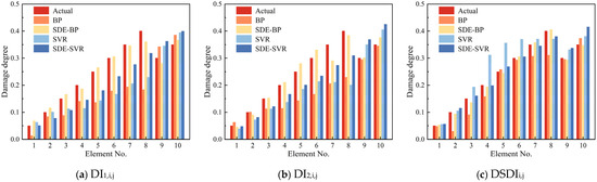
Figure 11. Prediction diagram of damage degree.

Table 5. Damage prediction error of BP and SVR algorithms.

Damage Index	BP Algorithm			SVR Algorithm
	MAE	RMSE	Accuracy Rate	MAE	RMSE	Accuracy Rate
DI1,i,j	0.08582	0.10536	63.55%	0.07004	0.09364	73.23%
DI2,i,j	0.07013	0.09363	73.23%	0.06408	0.08763	74.69%
DSDIi,j	0.03475	0.04545	81.82%	0.04293	0.05695	80.95%

Table 6. Damage prediction error of DE-BP and DE-SVR algorithms.

Damage Index	DE-BP Algorithm			DE-SVR Algorithm
	MAE	RMSE	Accuracy Rate	MAE	RMSE	Accuracy Rate
DI1,i,j	0.05901	0.07082	76.93%	0.06145	0.07217	75.26%
DI2,i,j	0.04351	0.06867	81.34%	0.04496	0.06921	79.68%
DSDIi,j	0.03982	0.04603	85.29%	0.04054	0.04958	83.55%

Table 7. Damage prediction error of SDE-BP and SDE-SVR algorithms.

Damage Index	SDE-BP Algorithm			SDE-SVR Algorithm
	MAE	RMSE	Accuracy Rate	MAE	RMSE	Accuracy Rate
DI1,i,j	0.01926	0.02576	89.98%	0.04245	0.05176	82.56%
DI2,i,j	0.01662	0.01815	92.26%	0.04081	0.04892	84.34%
DSDIi,j	0.00628	0.00693	96.54%	0.02036	0.02685	88.57%

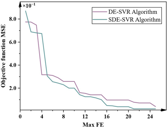
Figure 12. Convergence curve of SDE and original DE algorithms for tuning parameters of SVR model.

To effectively assess the recognition performance of different algorithms under varying damage conditions, this study selects the Mean Absolute Error (MAE) and Root Mean Squared Error (RMSE) as evaluation metrics. The corresponding formulas are as follows:

$$MAE={\displaystyle \frac{1}{n}}{\displaystyle \sum _{i=1}^n\left|\widehat{y_i}-y_i\right|}$$

(28)

$$RMSE=\sqrt{{\displaystyle \frac{1}{n}}{\displaystyle \sum _{i=1}^n{\left(\widehat{y_i}-y_i\right)}^2}}$$

(29)

In the equation, y_i denotes the actual value, while $\widehat{y_i}$ represents the predicted value.

As shown in Figure 11 and Figure 12 and Table 5, Table 6 and Table 7,

(1)

The performance of the BP and SDE-BP algorithms on the damage identification indices DI_1,i,j, DI_2,i,j, and the data fusion index DSDI_i,j demonstrates that SDE-BP significantly outperforms BP. Specifically, the accuracy of SDE-BP for DI_1,i,j increased from 63.55% to 89.95%, with the MAE and RMSE reduced to 0.01926 and 0.02576, respectively. For DI_2,i,j, accuracy improved to 92.26%, with the MAE and RMSE decreasing to 0.01662 and 0.01815. For DSDI_i,j, accuracy reached 96.54%, with the MAE and RMSE reduced to 0.00628 and 0.00693. Similar enhancements were observed in SVR neural networks following SDE optimization, confirming the generalized efficacy of the SDE framework for algorithmic improvement.

(2)

A comparison of predicted and actual damage severity values using BP and SVR reveals significant fluctuations in relative error, indicating suboptimal prediction performance. However, after SDE optimization, the relative error stabilizes considerably, further validating the effectiveness of the SDE optimization algorithm.

(3)

A comprehensive comparative evaluation of six machine learning architectures (SDE-BP, SDE-SVR, DE-BP, DE-SVR, BP, SVR) reveals that the proposed SDE-BP framework demonstrates superior predictive capability across all evaluation metrics (DI_1,i,j, DI_2,i,j, DSDIᵢ_,ⱼ), achieving peak accuracy values of 89.98%, 92.26%, and 96.54%, respectively. Although optimization occasionally results in lower accuracy for different indicators, the optimized algorithm generally outperforms the SDE pre-optimized version in terms of accuracy when evaluated on the same indicator.

(4)

The adaptive mutation operator in SDE enables dynamic balance between global exploration and local exploitation. This contrasts with DE’s fixed mutation strategy, which exhibits slower convergence and higher probability of premature convergence to suboptimal solutions.

(5)

SDE-SVR achieves convergence in 21 iterations (RMSE = 0.02685) compared to DE-SVR’s 25 iterations (RMSE = 0.04958), representing 16.00% faster convergence rate and 5.67% higher final accuracy (88.57% vs. 83.55%). These metrics collectively demonstrate significantly enhanced optimization efficiency through SDE implementation.

To comprehensively evaluate the robustness and efficiency of the SDE-optimized models, this study compares their performance with XGBoost (XGB), convolutional neural networks (CNN), and Long Short-Term Memory Networks (LSTMs). The evaluation considers key metrics, including the MAE, RMSE, accuracy rate, training time, and prediction time. The results are summarized in Table 8.

Table 8. Comparison of the performance of SDE-optimized models against other algorithms.

Algorithms	DSDIi,j
	MAE	RMSE	Accuracy Rate	Training Time (s)	Prediction Time (s)
XGBoost	0.02315	0.03041	86.92%	250.25	0.12
CNN	0.01987	0.02458	90.35%	480.73	0.22
LSTM	0.01894	0.02372	91.57%	520.89	0.35
SDE-SVR	0.02036	0.02685	88.57%	380.42	0.18
SDE-BP	0.00628	0.00693	96.54%	360.83	0.15

(1)

The SDE-optimized models (SDE-BP and SDE-SVR) exhibit superior performance in terms of the MAE and RMSE. Specifically, SDE-BP achieves an exceptionally low MAE of 0.00628 and RMSE of 0.00693, whereas XGBoost yields significantly higher errors (MAE = 0.03041, RMSE = 0.02315), indicating reduced accuracy in damage identification. Regarding classification accuracy, SDE-BP attains 96.54%, outperforming CNN (90.35%) and LSTM (91.57%). Although CNN and LSTM improve upon XGBoost, their longer training times remain a drawback.

(2)

In terms of training time, SDE-BP completes training in just 360.83 s, substantially faster than LSTM (520.89 s) and the CNN (480.73 s). SDE-SVR also performs efficiently, requiring 380.42 s for training and just 0.18 s for prediction, striking a favorable balance between accuracy and computational cost. In contrast, the CNN and LSTM demand significantly higher computational resources, with training times of 480.73 s and 520.89 s, respectively.

4.4. Sensitivity Analysis and Computational Efficiency

4.4.1. Sensitivity Analysis

To evaluate the impact of different threshold values in the fusion process on the accuracy of damage identification, a sensitivity analysis of the threshold values in the fusion process was conducted. The threshold values were systematically varied within a defined range, and the damage identification process was re-run for each value using the same experimental data.

The results of the sensitivity analysis indicate that the accuracy of damage identification is sensitive to the choice of threshold values. Specifically, lower threshold values increased the sensitivity to minor damage but also increased the risk of false positives. Higher threshold values improved the robustness of the method by reducing false positives but slightly decreased the sensitivity to minor damage. An optimal threshold value provided a good balance between sensitivity and robustness, achieving the highest accuracy in damage identification.

4.4.2. Computational Efficiency and Accuracy

The SDE-optimized models (SDE-BP and SDE-SVR) exhibit significantly higher accuracy in damage identification, as shown in Table 5 and Table 7. However, this enhanced accuracy comes at the expense of increased computational time. As illustrated in Table 9, the SDE-optimized models require more time for training compared to the non-optimized models. Specifically, the training time for SDE-BP and SDE-SVR is approximately three times longer than that for BP and SVR, respectively. This additional computational time primarily results from the iterative optimization process of the SDE algorithm, which dynamically adjusts model weights and thresholds to optimize performance. In terms of prediction time, the SDE-optimized models also show slightly longer prediction times compared to the non-optimized models. However, the difference in prediction time is relatively minor and may not pose a significant concern in many practical applications. Therefore, the trade-offs between computational efficiency and accuracy must be carefully considered when selecting the appropriate model for structural damage identification.

Table 9. Computational time for different models.

Model	Training Time (s)	Prediction Time (s)	Accuracy Rate
BP	121.73	0.10	81.82%
SVR	135.26	0.11	80.95%
SDE-BP	360.83	0.15	96.54%
SDE-SVR	380.42	0.18	88.57%

5. Experimental Validation

5.1. Experimental Setup

To assess the applicability of the proposed method in engineering applications, this study selected Q500 steel plate beams as the primary subject. Due to experimental constraints, the focus is on evaluating the damage location identification performance of the indicators DI_1,i,j, DI_2,i,j, and DSDI_i,j, rather than performing quantitative prediction analysis. Experimental Parameters: The steel plate beam has a total length of L = 2350 mm and a cross-sectional dimension of b × h = 100 × 8 mm². The beam is divided into 35 elements and 36 nodes within a span of 1750 mm, using a reference length of 50 mm. The density is ρ = 7698 kg/m³, and the elastic modulus is E = 2.0795 × 10⁸ KN/m².

Experimental Setup: The experimental equipment includes NV9812 piezo-resistive accelerometers, a YFF-1-64 impact hammer, a DLF-8 signal amplifier, Coinv DASP MAS modal and dynamic analysis software, an INV360U data acquisition system, a 220 V AC UPS voltage stabilizer, and a Dell laptop. The layout of the testing system and data acquisition, along with the accelerometer placement, is illustrated in Figure 13 and Figure 14.

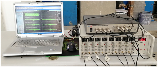
Figure 13. Diagram of testing and data acquisition system.

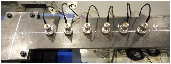
Figure 14. Layout diagram of acceleration sensors.

The experimental damage was simulated by symmetrically cutting the steel beam to represent various damage scenarios. The actual cutting configuration of the beam is shown in Figure 15, with a cutting width of 10 mm. The corresponding damage locations are provided in Table 10.

Figure 15. Cutting method.

Table 10. Damage conditions of simply supported steel beams.

Damage Condition	Location of Damage and Depth of Cut	Damage Degree (%)
DC1	Non-Damage Condition	0
DC2	30 cm and cut 2.5 cm	50
DC3	50 cm and cut 2 cm, 125 cm and cut 2.5 cm	40, 50
DC4	45 cm, 87.5 cm, 130 cm and cut 2 cm	40, 40, 40

5.2. Experimental Results

As shown in Figure 16,

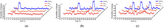
Figure 16. Identification of test conditions for steel plate girder: (a) damage identification for condition 2; (b) damage identification for condition 3; and (c) damage identification for condition 4.

(1)

The damage identification indicators DI_1,i,j, DI_2,i,j, and DSDI_i,j can accurately detect varying levels of damage at different locations on the experimental beam, including single, two-point, and multi-point damage scenarios. Furthermore, the damage severity is positively correlated with the peak value.

(2)

After D-S data fusion, the peak value probability at the damage locations increased, while the peak interference at non-damaged locations decreased. At non-damaged positions, fluctuations in the peak value were observed to varying extents, possibly due to environmental factors, measurement errors, or other influencing variables. However, these fluctuations did not significantly affect the damage identification accuracy.

6. Conclusions

This paper proposes a structural damage identification method based on data fusion and SDE algorithm optimization, grounded in the fundamental concepts of curvature mode, D-S evidence theory, and the Differential Evolution algorithm. Through numerical simulations and experimental validation on a simply supported beam, the following conclusions are drawn:

(1)

The proposed indicators DI_1,i,j, DI_2,i,j, and DSDI_i,j accurately identify single-location and multi-location damage on the simply supported beam. Compared to the first two indicators, the fused indicator DSDI_i,j demonstrates superior recognition performance and robustness.

(2)

The accuracy of the damage identification improves, and the error rate decreases with the use of SDE-optimized BP and SVR algorithms, enabling the high-precision prediction of damage levels on the simply supported beam.

(3)

The damage identification indicators DI_1,i,j, DI_2,i,j, and DSDI_i,j accurately detect varying damage levels under different conditions, with peak values positively correlated to damage severity. The experimental results confirm that the proposed method performs effectively in the engineering context of the simply supported beam.

However, this paper primarily focuses on simply supported beam structures. Future research will

(1)

Extend this method to truss and continuous beam bridges, focusing on optimizing sensor networks for complex geometries, recalibrating modal weights for boundary condition sensitivity, and improving computational efficiency for large-scale systems.

(2)

Validate the adaptability of the proposed method. Although this study centers on steel beams, its reliance on stiffness-dependent curvature modes and adaptive optimization principles suggests broader applicability to concrete and composite structures.

(3)

Validate the feasibility of implementing our method in real-time SHM systems.

References

- Yan, A.; Golinval, J.C. Structural Damage Localization by Combining Flexibility and Stiffness Methods. Eng. Struct. 2005, 27, 1752–1761. [Google Scholar] [CrossRef]
- Yang, Q.W.; Sun, B.X. Structural Damage Identification Based on Best Achievable Flexibility Change. Appl. Math. Modell. 2011, 35, 5217–5224. [Google Scholar] [CrossRef]
- Lee, E.T.; Eun, H.C. Damage Identification of a Frame Structure Model Based on the Response Variation Depending on Additional Mass. Eng. Comput. 2015, 31, 737–747. [Google Scholar] [CrossRef]
- Hou, J.; Li, Z.; Zhang, Q.; Jankowski, Ł.; Zhang, H. Local Mass Addition and Data Fusion for Structural Damage Identification Using Approximate Models. Int. J. Struct. Stab. Dyn. 2020, 20, 2050124. [Google Scholar] [CrossRef]
- Pandey, A.K.; Biswas, M.; Samman, M.M. Damage Detection from Changes in Curvature Mode Shapes. J. Sound Vib. 1991, 145, 321–332. [Google Scholar] [CrossRef]
- Ren, X.; Meng, Z. Damage Identification for Timber Structure Using Curvature Mode and Wavelet Transform. Structures 2024, 60, 105798. [Google Scholar] [CrossRef]
- Huang, T.; Liang, T.; Chen, L. A Comparative Analysis of Damage Identification Methods Based on Multi-Channel Data Fusion and Convolutional Neural Network for Frame Structures. Structures 2024, 61, 106076. [Google Scholar] [CrossRef]
- Jaramillo, V.H.; Ottewill, J.R.; Dudek, R.; Lepiarczyk, D.; Pawlik, P. Condition Monitoring of Distributed Systems Using Two-Stage Bayesian Inference Data Fusion. Mech. Syst. Signal Proc. 2017, 87, 91–110. [Google Scholar] [CrossRef]
- Sadeghi, F.; Yu, Y.; Zhu, X.; Li, J. Damage Identification of Steel-Concrete Composite Beams Based on Modal Strain Energy Changes Through General Regression Neural Network. Eng. Struct. 2021, 244, 112824. [Google Scholar] [CrossRef]
- Li, M.; Jia, D.; Wu, Z.; Qiu, S.; He, W. Structural Damage Identification Using Strain Mode Differences by the iFEM Based on the Convolutional Neural Network (CNN). Mech. Syst. Signal Proc. 2022, 165, 108289. [Google Scholar] [CrossRef]
- Miao, B.; Wang, M.; Yang, S.; Luo, Y.; Yang, C. An Optimized Damage Identification Method of Beam Using Wavelet and Neural Network. Engineering 2020, 12, 748. [Google Scholar] [CrossRef]
- Ghiasi, R.; Torkzadeh, P.; Noori, M. A Machine-Learning Approach for Structural Damage Detection Using Least Square Support Vector Machine Based on a New Combinational Kernel Function. Struct. Health Monit. 2016, 15, 302–316. [Google Scholar] [CrossRef]
- Yan, B.; Cui, Y.; Zhang, L.; Zhang, C.; Yang, Y.; Bao, Z.; Ning, G. Beam Structure Damage Identification Based on BP Neural Network and Support Vector Machine. Math. Prob. Eng. 2014, 2014, 850141. [Google Scholar] [CrossRef]
- Dessi, D.; Camerlengo, G. Damage Identification Techniques via Modal Curvature Analysis: Overview and Comparison. Mech. Syst. Signal Proc. 2015, 52, 181–205. [Google Scholar] [CrossRef]
- Guyon, I.; Elisseeff, A. An Introduction to Variable and Feature Selection. J. Mach. Learn. Res. 2003, 3, 1157–1182. [Google Scholar] [CrossRef]
- Dempster, A.P. Upper and Lower Probabilities Induced by a Multivalued Mapping. Ann. Math. Stat. 1967, 38, 325–339. [Google Scholar] [CrossRef]
- Bao, Y.; Li, H.; An, Y.; Ou, J. Dempster–Shafer Evidence Theory Approach to Structural Damage Detection. Struct. Health Monit. 2012, 11, 13–26. [Google Scholar] [CrossRef]
- Storn, R.; Price, K. Differential Evolution—A Simple and Efficient Heuristic for Global Optimization over Continuous Spaces. J. Glob. Optim. 1997, 11, 341–359. [Google Scholar] [CrossRef]
- Pant, M.; Zaheer, H.; Garcia-Hernandez, L.; Abraham, A. Differential Evolution: A Review of More Than Two Decades of Research. Eng. Appl. Artif. Intell. 2020, 90, 103479. [Google Scholar] [CrossRef]
- Wang, L.; Zeng, Y.; Chen, T. Back Propagation Neural Network with Adaptive Differential Evolution Algorithm for Time Series Forecasting. Expert Syst. Appl. 2015, 42, 855–863. [Google Scholar] [CrossRef]
- Leema, N.; Nehemiah, H.K.; Kannan, A. Neural Network Classifier Optimization Using Differential Evolution with Global Information and Back Propagation Algorithm for Clinical Datasets. Appl. Soft Comput. 2016, 49, 834–844. [Google Scholar] [CrossRef]
- Ding, Y.; Yao, X.; Wang, S.; Zhao, X. Structural Damage Assessment Using Improved Dempster-Shafer Data Fusion Algorithm. Earthq. Eng. Eng. Vibr. 2019, 18, 395–408. [Google Scholar] [CrossRef]
- Fan, W.; Qiao, P. Vibration-Based Damage Identification Methods: A Review and Comparative Study. Struct. Health Monit. 2011, 10, 83–111. [Google Scholar] [CrossRef]
Disclaimer/Publisher’s Note: The statements, opinions and data contained in all publications are solely those of the individual author(s) and contributor(s) and not of MDPI and/or the editor(s). MDPI and/or the editor(s) disclaim responsibility for any injury to people or property resulting from any ideas, methods, instructions or products referred to in the content. |
© 2025 by the authors. Licensee MDPI, Basel, Switzerland. This article is an open access article distributed under the terms and conditions of the Creative Commons Attribution (CC BY) license (https://creativecommons.org/licenses/by/4.0/).