
TS-HTFA: Advancing Time-Series Forecasting via Hierarchical Text-Free Alignment with Large Language Models
 , , , , , , , and
Abstract
1. Introduction
- A hierarchical text-free alignment framework is proposed, supported by novel probabilistic analysis, enabling comprehensive alignment across input, intermediate, and output spaces.
- Dynamic adaptive gating is integrated into the input embedding layer to align time-series data with textual representations and generate virtual text embeddings. Additionally, a novel combination of layerwise contrastive learning and optimal transport loss is introduced to align intermediate representations and output distributions.
- The proposed framework is validated through extensive experiments, achieving competitive or state-of-the-art performance on both long-term and short-term forecasting tasks across multiple benchmark datasets.
2. Related Work
2.1. Time-Series Forecasting
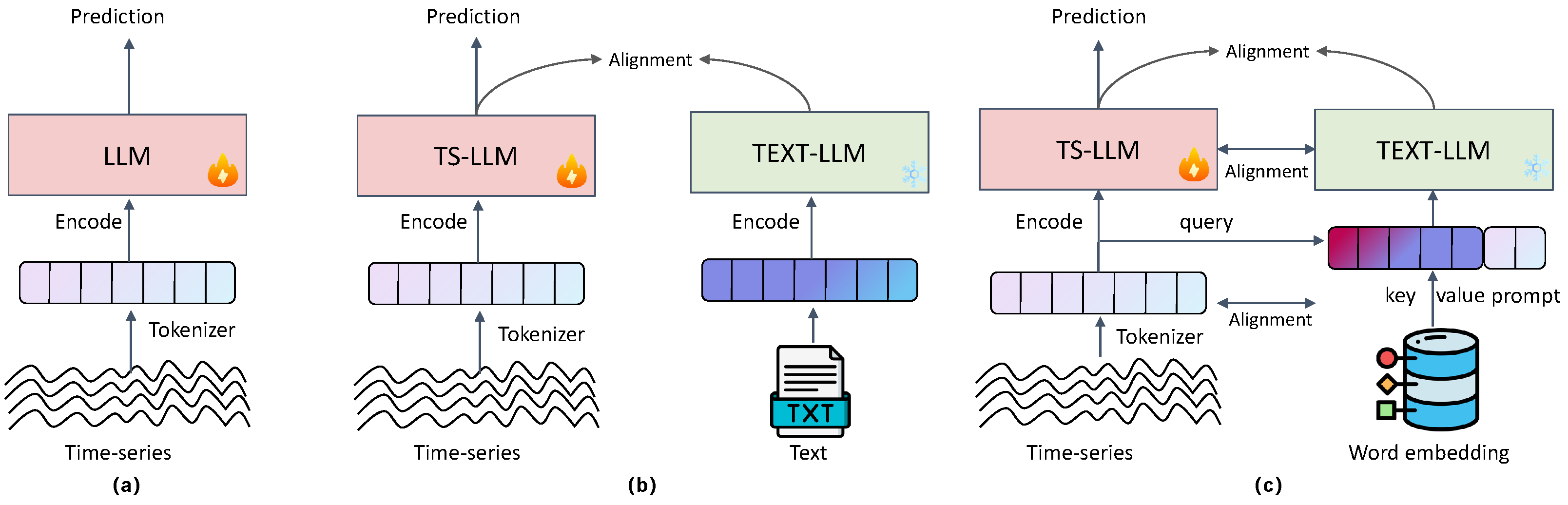
2.2. LLMs for Time-Series Forecasting
2.3. Cross-Modal Learning
3. Preliminaries
3.1. Theoretical Analysis
3.2. Task Definition
3.3. List of Abbreviations
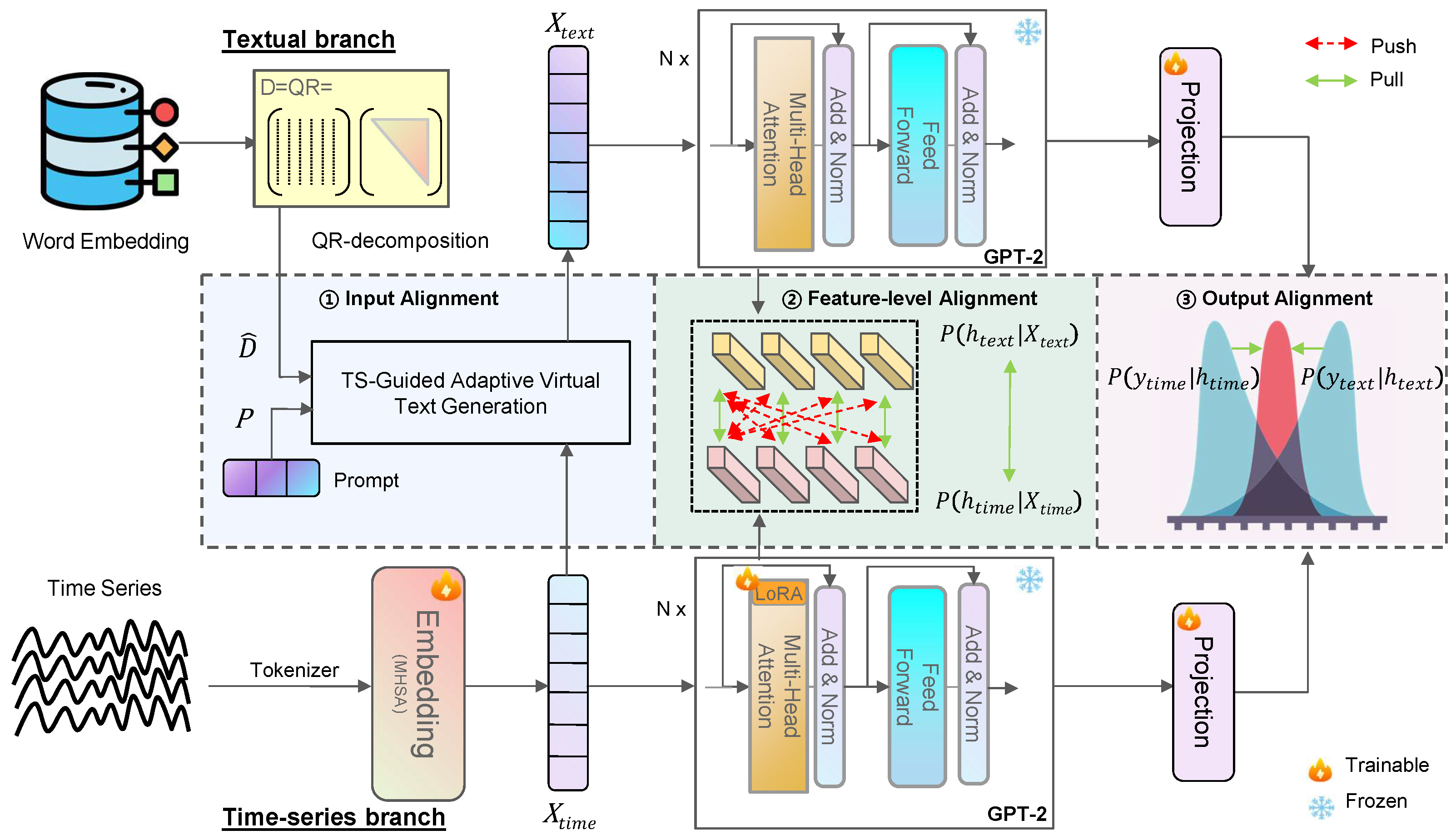
4. Method Overview
4.1. TS-Guided Adaptive Virtual Text Generation in Input Alignment
4.1.1. Time-Series Encoding
4.1.2. QR-Decomposed Word Embedding
4.1.3. Virtual Text Generation via Dynamic Adaptive Gating
4.2. Layerwise Contrastive Learning for Intermediate Network Alignment
4.3. Optimal Transport-Driven Output Layer Alignment
4.4. Total Loss Function for Cross-Modal Distillation
5. Experiments
5.1. Experimental Setups
5.1.1. Implementation Details
5.1.2. Baselines
5.1.3. Datasets
5.1.4. Evaluation Metrics
5.2. Main Results
5.2.1. Long-Term Forecasting
5.2.2. Short-Term Forecasting
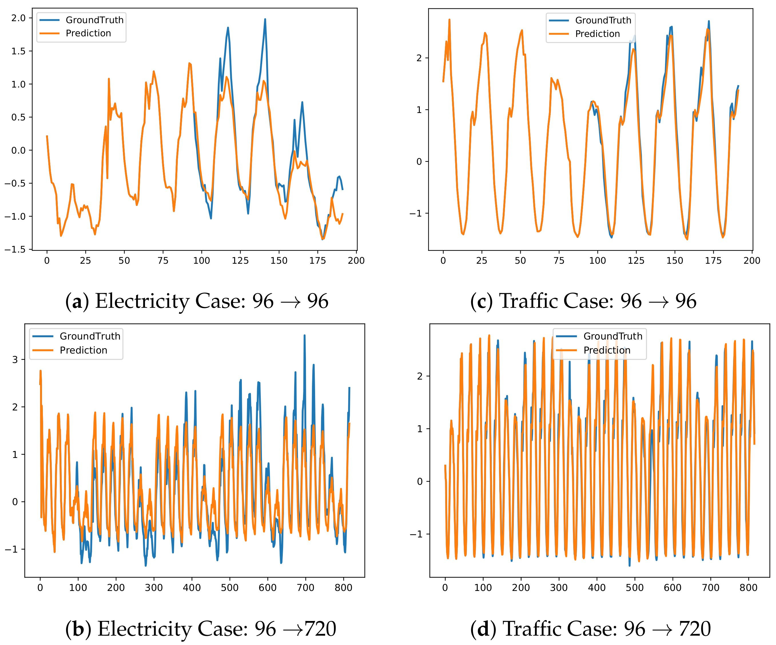
5.2.3. Visualization
5.3. Ablation Studies
5.3.1. Ablation on Different Stage Alignment
5.3.2. Ablation on Different Reduction Methods
5.3.3. Hyperparameter Study
5.4. Theoretical Complexity Analysis and Practical Model Efficiency
6. Discussion
7. Conclusions
- Independence from paired textual data: TS-HTFA effectively leverages the representational power of LLMs without requiring annotated textual descriptions, reducing data preparation effort and enhancing adaptability.
- Enhanced alignment between numerical and linguistic models: By generating virtual text tokens, TS-HTFA allows LLMs to fully utilize their pretrained capabilities while maintaining the structural integrity of the time-series data.
- Lower computational cost: During inference, the linguistic branch is discarded, significantly reducing computational overhead compared with traditional LLM-based methods.
Author Contributions
Funding
Data Availability Statement
Conflicts of Interest
References
- Zhang, C.; Sjarif, N.N.A.; Ibrahim, R. Deep Learning Models for Price Forecasting of Financial Time Series: A Review of Recent Advancements: 2020–2022. Wiley Interdiscip. Rev. Data Min. Knowl. Discov. 2024, 14, e1519. [Google Scholar] [CrossRef]
- Gao, P.; Liu, T.; Liu, J.W.; Lu, B.L.; Zheng, W.L. Multimodal Multi-View Spectral-Spatial-Temporal Masked Autoencoder for Self-Supervised Emotion Recognition. In Proceedings of the ICASSP 2024—2024 IEEE International Conference on Acoustics, Speech and Signal Processing (ICASSP), Seoul, Republic of Korea, 14–19 April 2024; pp. 1926–1930. [Google Scholar]
- Liu, P.; Wu, B.; Li, N.; Dai, T.; Lei, F.; Bao, J.; Jiang, Y.; Xia, S.T. Wftnet: Exploiting global and local periodicity in long-term time series forecasting. In Proceedings of the ICASSP 2024—2024 IEEE International Conference on Acoustics, Speech and Signal Processing (ICASSP), Seoul, Republic of Korea, 14–19 April 2024; pp. 5960–5964. [Google Scholar]
- Pan, J.; Ji, W.; Zhong, B.; Wang, P.; Wang, X.; Chen, J. DUMA: Dual mask for multivariate time series anomaly detection. IEEE Sensors J. 2022, 23, 2433–2442. [Google Scholar] [CrossRef]
- Bai, S.; Kolter, J.Z.; Koltun, V. An empirical evaluation of generic convolutional and recurrent networks for sequence modeling. arXiv 2018, arXiv:1803.01271. [Google Scholar]
- Wang, H.; Peng, J.; Huang, F.; Wang, J.; Chen, J.; Xiao, Y. MICN: Multi-scale local and global context modeling for long-term series forecasting. In Proceedings of the International Conference on Learning Representations, Virtual Event, 25–29 April 2022. [Google Scholar]
- Wu, H.; Hu, T.; Liu, Y.; Zhou, H.; Wang, J.; Long, M. TimesNet: Temporal 2D-Variation Modeling for General Time Series Analysis. In Proceedings of the The Eleventh International Conference on Learning Representations, Virtual Event, 25–29 April 2022. [Google Scholar]
- Zeng, A.; Chen, M.; Zhang, L.; Xu, Q. Are transformers effective for time series forecasting? In Proceedings of the AAAI Conference on Artificial Intelligence, Washington, DC, USA, 7–14 February 2023; Volume 37, pp. 11121–11128. [Google Scholar] [CrossRef]
- Das, A.; Kong, W.; Leach, A.; Sen, R.; Yu, R. Long-term Forecasting with TiDE: Time-series Dense Encoder. arXiv 2023, arXiv:2304.08424. [Google Scholar]
- Xue, H.; Salim, F.D. Promptcast: A new prompt-based learning paradigm for time series forecasting. IEEE Trans. Knowl. Data Eng. 2023, 36, 6851–6864. [Google Scholar] [CrossRef]
- Cao, D.; Jia, F.; Arik, S.O.; Pfister, T.; Zheng, Y.; Ye, W.; Liu, Y. Tempo: Prompt-based generative pre-trained transformer for time series forecasting. arXiv 2023, arXiv:2310.04948. [Google Scholar]
- Chang, C.; Peng, W.C.; Chen, T.F. Llm4ts: Two-stage fine-tuning for time-series forecasting with pre-trained llms. arXiv 2023, arXiv:2308.08469. [Google Scholar]
- Jin, M.; Wang, S.; Ma, L.; Chu, Z.; Zhang, J.Y.; Shi, X.; Chen, P.Y.; Liang, Y.; Li, Y.F.; Pan, S.; et al. Time-llm: Time series forecasting by reprogramming large language models. arXiv 2023, arXiv:2310.01728. [Google Scholar]
- Sun, C.; Li, Y.; Li, H.; Hong, S. TEST: Text prototype aligned embedding to activate LLM’s ability for time series. arXiv 2023, arXiv:2308.08241. [Google Scholar]
- Wang, Z.; Ji, H. Open vocabulary electroencephalography-to-text decoding and zero-shot sentiment classification. In Proceedings of the AAAI Conference on Artificial Intelligence, Online, 22 February–1 March 2022; Volume 36, pp. 5350–5358. [Google Scholar]
- Qiu, J.; Han, W.; Zhu, J.; Xu, M.; Weber, D.; Li, B.; Zhao, D. Can brain signals reveal inner alignment with human languages? In Proceedings of the Findings of the Association for Computational Linguistics: EMNLP 2023, Singapore, 6–10 December 2023; pp. 1789–1804. [Google Scholar]
- Li, J.; Liu, C.; Cheng, S.; Arcucci, R.; Hong, S. Frozen language model helps ECG zero-shot learning. In Proceedings of the Medical Imaging with Deep Learning, PMLR, Paris, France, 3–5 July 2024; pp. 402–415. [Google Scholar]
- Jia, F.; Wang, K.; Zheng, Y.; Cao, D.; Liu, Y. GPT4MTS: Prompt-based Large Language Model for Multimodal Time-series Forecasting. In Proceedings of the AAAI Conference on Artificial Intelligence, Vancouver, BC, Canada, 26–27 February 2024; Volume 38, pp. 23343–23351. [Google Scholar]
- Yu, H.; Guo, P.; Sano, A. ECG Semantic Integrator (ESI): A Foundation ECG Model Pretrained with LLM-Enhanced Cardiological Text. arXiv 2024, arXiv:2405.19366. [Google Scholar]
- Kim, J.W.; Alaa, A.; Bernardo, D. EEG-GPT: Exploring Capabilities of Large Language Models for EEG Classification and Interpretation. arXiv 2024, arXiv:2401.18006. [Google Scholar]
- Zhou, T.; Ma, Z.; Wen, Q.; Wang, X.; Sun, L.; Jin, R. FEDformer: Frequency enhanced decomposed transformer for long-term series forecasting. In Proceedings of the International Conference on Machine Learning, PMLR, Baltimore, MD, USA, 17–23 July 2022; pp. 27268–27286. [Google Scholar]
- Nie, Y.; Nguyen, N.H.; Sinthong, P.; Kalagnanam, J. A Time Series is Worth 64 Words: Long-term Forecasting with Transformers. In Proceedings of the International Conference on Learning Representations, Kigali, Rwanda, 1–5 May 2023; 5 May 2023. [Google Scholar]
- Zhang, Y.; Yan, J. Crossformer: Transformer utilizing cross-dimension dependency for multivariate time series forecasting. In Proceedings of the International Conference on Learning Representations, Kigali, Rwanda, 1–5 May 2023. [Google Scholar]
- Liu, Y.; Hu, T.; Zhang, H.; Wu, H.; Wang, S.; Ma, L.; Long, M. itransformer: Inverted transformers are effective for time series forecasting. arXiv 2023, arXiv:2310.06625. [Google Scholar]
- Zhou, T.; Niu, P.; Wang, X.; Sun, L.; Jin, R. One Fits All: Power General Time Series Analysis by Pretrained LM. arXiv 2023, arXiv:2302.11939. [Google Scholar]
- Pan, Z.; Jiang, Y.; Garg, S.; Schneider, A.; Nevmyvaka, Y.; Song, D. S2 IP-LLM: Semantic Space Informed Prompt Learning with LLM for Time Series Forecasting. In Proceedings of the Forty-First International Conference on Machine Learning, Vienna, Austria, 21–27 July 2024. [Google Scholar]
- Liu, X.; Hu, J.; Li, Y.; Diao, S.; Liang, Y.; Hooi, B.; Zimmermann, R. Unitime: A language-empowered unified model for cross-domain time series forecasting. In Proceedings of the ACM on Web Conference 2024, Singapore, 13–17 May 2024; pp. 4095–4106. [Google Scholar]
- Liu, C.; Xu, Q.; Miao, H.; Yang, S.; Zhang, L.; Long, C.; Li, Z.; Zhao, R. TimeCMA: Towards LLM-Empowered Time Series Forecasting via Cross-Modality Alignment. arXiv 2025, arXiv:2406.01638. [Google Scholar]
- Hu, Y.; Li, Q.; Zhang, D.; Yan, J.; Chen, Y. Context-Alignment: Activating and Enhancing LLM Capabilities in Time Series. In Proceedings of the International Conference on Learning Representations, Singapore, 24–28 April 2025. [Google Scholar]
- Liu, P.; Guo, H.; Dai, T.; Li, N.; Bao, J.; Ren, X.; Jiang, Y.; Xia, S.T. CALF: Aligning LLMs for Time Series Forecasting via Cross-modal Fine-Tuning. arXiv 2025, arXiv:2403.07300. [Google Scholar]
- Shen, J.; Li, L.; Dery, L.M.; Staten, C.; Khodak, M.; Neubig, G.; Talwalkar, A. Cross-Modal Fine-Tuning: Align then Refine. In Proceedings of the International Conference on Machine Learning, Honolulu, HI, USA, 23–29 July 2023. [Google Scholar]
- Chen, P.Y. Model Reprogramming: Resource-Efficient Cross-Domain Machine Learning. In Proceedings of the AAAI Conference on Artificial Intelligence, Vancouver, BC, Canada, 20–27 February 2024; Volume 38, pp. 22584–22591. [Google Scholar]
- Pang, Z.; Xie, Z.; Man, Y.; Wang, Y.X. Frozen Transformers in Language Models Are Effective Visual Encoder Layers. In Proceedings of the Twelfth International Conference on Learning Representations, Vienna, Austria, 7–11 May 2024. [Google Scholar]
- Lai, Z.; Wu, J.; Chen, S.; Zhou, Y.; Hovakimyan, N. Residual-based Language Models are Free Boosters for Biomedical Imaging Tasks. In Proceedings of the IEEE/CVF Conference on Computer Vision and Pattern Recognition, Seattle, WA, USA, 16–22 June 2024; pp. 5086–5096. [Google Scholar]
- Jin, Y.; Hu, G.; Chen, H.; Miao, D.; Hu, L.; Zhao, C. Cross-Modal Distillation for Speaker Recognition. In Proceedings of the AAAI Conference on Artificial Intelligence, Vancouver, BC, Canada, 7–14 February 2023. [Google Scholar]
- Vinod, R.; Chen, P.Y.; Das, P. Reprogramming Pretrained Language Models for Protein Sequence Representation Learning. arXiv 2023, arXiv:2301.02120. [Google Scholar]
- Zhao, Z.; Fan, W.; Li, J.; Liu, Y.; Mei, X.; Wang, Y.; Wen, Z.; Wang, F.; Zhao, X.; Tang, J.; et al. Recommender systems in the era of large language models (llms). IEEE Trans. Knowl. Data Eng. 2024. [Google Scholar] [CrossRef]
- Hu, E.J.; Shen, Y.; Wallis, P.; Allen-Zhu, Z.; Li, Y.; Wang, S.; Wang, L.; Chen, W. Lora: Low-rank adaptation of large language models. arXiv 2021, arXiv:2106.09685. [Google Scholar]
- Lee, Y.L.; Tsai, Y.H.; Chiu, W.C.; Lee, C.Y. Multimodal prompting with missing modalities for visual recognition. In Proceedings of the IEEE/CVF Conference on Computer Vision and Pattern Recognition, Vancouver, BC, Canada, 17–24 June 2023; pp. 14943–14952. [Google Scholar]
- Villani, C. Topics in Optimal Transportation; American Mathematical Society: Providence, RI, USA, 2021; Volume 58. [Google Scholar]
- Cuturi, M. Sinkhorn Distances: Lightspeed Computation of Optimal Transport. Adv. Neural Inf. Process. Syst. 2013, 26. [Google Scholar]
- Liu, Y.; Qin, G.; Huang, X.; Wang, J.; Long, M. Autotimes: Autoregressive time series forecasters via large language models. arXiv 2024, arXiv:2402.02370. [Google Scholar]
- Radford, A.; Wu, J.; Child, R.; Luan, D.; Amodei, D.; Sutskever, I. Language models are unsupervised multitask learners. OpenAI Blog 2019, 1, 9. [Google Scholar]
- Kingma, D.P.; Ba, J. Adam: A method for stochastic optimization. arXiv 2014, arXiv:1412.6980. [Google Scholar]
- Wu, H.; Xu, J.; Wang, J.; Long, M. Autoformer: Decomposition Transformers with Auto-Correlation for Long-Term Series Forecasting. In Proceedings of the Advances in Neural Information Processing Systems, Red Hook, NY, USA, 6–14 December 2021. [Google Scholar]
- Woo, G.; Liu, C.; Sahoo, D.; Kumar, A.; Hoi, S.C.H. ETSformer: Exponential Smoothing Transformers for Time-series Forecasting. arXiv 2022, arXiv:2202.01381. [Google Scholar]
- Tan, M.; Merrill, M.; Gupta, V.; Althoff, T.; Hartvigsen, T. Are language models actually useful for time series forecasting? In Proceedings of the NeurIPS, Vancouver, BC, Canada, 9–15 December 2024.
- Challu, C.; Olivares, K.G.; Oreshkin, B.N.; Garza, F.; Mergenthaler, M.; Dubrawski, A. N-HiTS: Neural Hierarchical Interpolation for Time Series Forecasting. arXiv 2022, arXiv:2201.12886. [Google Scholar]
- Oreshkin, B.N.; Carpov, D.; Chapados, N.; Bengio, Y. N-BEATS: Neural basis expansion analysis for interpretable time series forecasting. arXiv 2019, arXiv:1905.10437. [Google Scholar]
- Qiu, X.; Hu, J.; Zhou, L.; Wu, X.; Du, J.; Zhang, B.; Guo, C.; Zhou, A.; Jensen, C.S.; Sheng, Z.; et al. TFB: Towards Comprehensive and Fair Benchmarking of Time Series Forecasting Methods. arXiv 2024, arXiv:2403.20150. [Google Scholar] [CrossRef]
- Makridakis, S.; Spiliotis, E.; Assimakopoulos, V. The M4 Competition: Results, Findings, Conclusion and Way Forward. Int. J. Forecast. 2018, 34, 802–808. [Google Scholar] [CrossRef]
- Jiang, Y.; Pan, Z.; Zhang, X.; Garg, S.; Schneider, A.; Nevmyvaka, Y.; Song, D. Empowering Time Series Analysis with Large Language Models: A Survey. arXiv 2024, arXiv:2402.03182. [Google Scholar]
- Jin, M.; Zhang, Y.; Chen, W.; Zhang, K.; Liang, Y.; Yang, B.; Wang, J.; Pan, S.; Wen, Q. Position: What Can Large Language Models Tell Us about Time Series Analysis. In Proceedings of the Forty-First International Conference on Machine Learning, Vienna, Austria, 21–27 July 2024. [Google Scholar]
- Guo, D.; Yang, D.; Zhang, H.; Song, J.; Zhang, R.; Xu, R.; Zhu, Q.; Ma, S.; Wang, P.; Bi, X.; et al. Deepseek-r1: Incentivizing reasoning capability in llms via reinforcement learning. arXiv 2025, arXiv:2501.12948. [Google Scholar]
- Kong, Y.; Yang, Y.; Wang, S.; Liu, C.; Liang, Y.; Jin, M.; Zohren, S.; Pei, D.; Liu, Y.; Wen, Q. Position: Empowering Time Series Reasoning with Multimodal LLMs. arXiv 2025, arXiv:2502.01477. [Google Scholar]


| Abbreviation | Full Term |
|---|---|
| TS-HTFA | Time-Series Hierarchical Feature-Text Alignment |
| TS-GAVTG | Time-Series Guided Adaptive Virtual Text Generation |
| LoRA | Low-Rank Adaptation |
| OT | Optimal Transport |
| QR | Orthogonal-Upper Triangular (QR Decomposition) |
| InfoNCE | Information Noise-Contrastive Estimation |
| LLM | Large Language Model |
| Model | Description |
|---|---|
| CALF [30] | Employs a cross-modal matching module with a two-stream architecture to mitigate modality gaps and align features. |
| DECA [29] | Leverages dual-scale context-alignment GNNs to align time-series data with linguistic components, enabling pretrained LLMs to contextualize and comprehend time-series data for enhanced performance. |
| TimeCMA [28] | Leverages LLM-based prompt embeddings and a dual-tower framework with late-stage cross-modality alignment for improved multivariate time-series forecasting. |
| S2IP-LLM [26] | Aligns time-series embeddings with pretrained semantic spaces using a tokenization module for temporal dynamics and semantic anchors for forecasting via cosine similarity in a joint space. |
| UniTime [27] | Utilizes domain instructions and a Language-TS Transformer for modality alignment while employing masking to address domain convergence speed imbalances. |
| TimeLLM [13] | Reprograms time-series tokens using multihead attention and fine-tunes pretrained LLMs with prefix prompting for time-series analysis. |
| GPT4TS [25] | Represents time-series data as patched tokens and fine-tunes GPT-2 [43] for various time-series tasks. |
| PatchTST [22] | Utilizes a Transformer-based model that segments data into patches and employs a channel-independent design to improve forecasting efficiency and performance. |
| iTransformer [24] | Captures multivariate correlations by applying attention and feed-forward networks to inverted time-series dimensions. |
| Crossformer [23] | Extracts segmentwise representations channel by channel and applies a two-stage attention mechanism to capture cross-temporal and cross-dimensional dependencies. |
| FEDformer [21] | Incorporates seasonal-trend decomposition and frequency-domain information into Transformers to improve efficiency and accuracy in time-series forecasting. |
| Autoformer [45] | Employs a decomposition architecture and Auto-Correlation mechanisms for efficient and accurate long-term forecasting. |
| ETSformer [46] | Integrates exponential smoothing into attention mechanisms, combining exponential smoothing attention and frequency attention for time-series forecasting. |
| PAttn, LTrsf [47] | Question the effectiveness of LLMs in time-series analysis. Evaluations with a standardized lookback window of 96 and the “Drop Last” option disabled during testing [50] reveal their potential limitations. |
| MICN [6] | Employs multiscale convolutions to capture temporal dependencies at different resolutions and models complex feature interactions for accurate forecasting. |
| TimesNet [7] | Transforms 1D time-series data into 2D representations, using TimesBlock with an inception module to capture intra- and inter-period relations for diverse tasks. |
| TiDE [9] | Combines temporal convolutional networks and recurrent neural networks to capture both short-term patterns and long-term dependencies effectively. |
| DLinear [8] | Models time-series data by decomposing and separately modeling trend and seasonal components using linear layers. |
| N-BEATS [49] | Models trend and seasonality components using backward and forward residual links for interpretable time-series forecasting. |
| N-HiTS [48] | Dynamically adjusts hierarchical structures to refine predictions, effectively handling multiple temporal resolutions. |
| Task | Dataset | Dim. | Series Length | Dataset Size | Frequency | Domain |
|---|---|---|---|---|---|---|
| ETTm1 | 7 | {96, 192, 336, 720} | (34,465, 11,521, 11,521) | 15 min | Temperature | |
| ETTm2 | 7 | {96, 192, 336, 720} | (34,465, 11,521, 11,521) | 15 min | Temperature | |
| Long-term | ETTh1 | 7 | {96, 192, 336, 720} | (8545, 2881, 2881) | 1 hour | Temperature |
| Forecasting | ETTh2 | 7 | {96, 192, 336, 720} | (8545, 2881, 2881) | 1 hour | Temperature |
| Electricity(ELC) | 321 | {96, 192, 336, 720} | (18,317, 2633, 5261) | 1 hour | Electricity | |
| Traffic | 862 | {96, 192, 336, 720} | (12,185, 1757, 3509) | 1 hour | Transportation | |
| Weather | 21 | {96, 192, 336, 720} | (36,792, 5271, 10,540) | 10 min | Weather | |
| M4-Yearly | 1 | 6 | (23,000, 0, 23,000) | Yearly | Demographic | |
| M4-Quarterly | 1 | 8 | (24,000, 0, 24,000) | Quarterly | Finance | |
| Short-term | M4-Monthly | 1 | 18 | (48,000, 0, 48,000) | Monthly | Industry |
| Forecasting | M4-Weakly | 1 | 13 | (359, 0, 359) | Weakly | Macro |
| M4-Daily | 1 | 14 | (4227, 0, 4227) | Daily | Micro | |
| M4-Hourly | 1 | 48 | (414, 0, 414) | Hourly | Other |
| Method | Source | Metric↓ | ETTm1 | ETTm2 | ETTh1 | ETTh2 | Weather | ELC | Traffic | 1st Count |
|---|---|---|---|---|---|---|---|---|---|---|
| TiDE [9] | TMLR’2023 | MSE | 0.412 | 0.289 | 0.445 | 0.611 | 0.271 | 0.251 | 0.760 | 0 |
| MAE | 0.406 | 0.326 | 0.432 | 0.550 | 0.320 | 0.344 | 0.473 | |||
| DLinear [8] | AAAI’2023 | MSE | 0.403 | 0.350 | 0.456 | 0.559 | 0.265 | 0.212 | 0.625 | 0 |
| MAE | 0.407 | 0.401 | 0.452 | 0.515 | 0.317 | 0.300 | 0.383 | |||
| MICN [6] | AAAI’2023 | MSE | 0.392 | 0.328 | 0.558 | 0.587 | 0.242 | 0.186 | 0.541 | 1 |
| MAE | 0.413 | 0.382 | 0.535 | 0.525 | 0.299 | 0.294 | 0.315 | |||
| TimesNet [7] | ICLR’2023 | MSE | 0.400 | 0.291 | 0.458 | 0.414 | 0.259 | 0.192 | 0.620 | 0 |
| MAE | 0.406 | 0.333 | 0.450 | 0.427 | 0.287 | 0.295 | 0.336 | |||
| FEDformer [21] | ICML’2022 | MSE | 0.448 | 0.305 | 0.440 | 0.437 | 0.309 | 0.214 | 0.610 | 0 |
| MAE | 0.452 | 0.349 | 0.460 | 0.449 | 0.360 | 0.327 | 0.376 | |||
| Crossformer [23] | ICLR’2023 | MSE | 0.502 | 1.216 | 0.620 | 0.942 | 0.259 | 0.244 | 0.550 | 0 |
| MAE | 0.502 | 0.707 | 0.572 | 0.684 | 0.315 | 0.334 | 0.304 | |||
| iTransformer [24] | ICLR’2024 | MSE | 0.407 | 0.291 | 0.455 | 0.381 | 0.257 | 0.178 | 0.428 | 0 |
| MAE | 0.411 | 0.335 | 0.448 | 0.405 | 0.279 | 0.270 | 0.282 | |||
| PatchTST [22] | ICLR’2023 | MSE | 0.381 | 0.285 | 0.450 | 0.366 | 0.258 | 0.216 | 0.555 | 1 |
| MAE | 0.395 | 0.327 | 0.441 | 0.394 | 0.280 | 0.304 | 0.361 | |||
| GPT4TS [25] | NeurIPS’2023 | MSE | 0.389 | 0.285 | 0.447 | 0.381 | 0.264 | 0.205 | 0.488 | 0 |
| MAE | 0.397 | 0.331 | 0.436 | 0.408 | 0.284 | 0.290 | 0.317 | |||
| TimeLLM [13] | ICLR’2024 | MSE | 0.410 | 0.296 | 0.460 | 0.389 | 0.274 | 0.223 | 0.541 | 0 |
| MAE | 0.409 | 0.340 | 0.449 | 0.408 | 0.290 | 0.309 | 0.358 | |||
| PAttn [47] | NeurIPS’2024 | MSE | 0.390 | 0.281 | 0.449 | 0.369 | 0.261 | 0.209 | 0.562 | 0 |
| MAE | 0.386 | 0.320 | 0.428 | 0.392 | 0.276 | 0.282 | 0.331 | |||
| LTrsf [47] | NeurIPS’2024 | MSE | 0.400 | 0.282 | 0.446 | 0.374 | 0.262 | 0.201 | 0.518 | 0 |
| MAE | 0.392 | 0.322 | 0.433 | 0.397 | 0.275 | 0.275 | 0.312 | |||
| UniTime [27] | WWW’2024 | MSE | 0.385 | 0.293 | 0.442 | 0.378 | 0.253 | 0.216 | 0.477 | 0 |
| MAE | 0.399 | 0.334 | 0.448 | 0.403 | 0.276 | 0.305 | 0.321 | |||
| TimeCMA [28] | AAAI’2025 | MSE | 0.380 | 0.275 | 0.423 | 0.372 | 0.250 | 0.174 | 0.451 | 3 |
| MAE | 0.392 | 0.323 | 0.431 | 0.397 | 0.276 | 0.269 | 0.297 | |||
| CALF [30] | AAAI’2025 | MSE | 0.395 | 0.281 | 0.432 | 0.349 | 0.250 | 0.175 | 0.439 | 2 |
| MAE | 0.390 | 0.321 | 0.428 | 0.382 | 0.274 | 0.265 | 0.281 | |||
| TS-HTFA (Ours ) | - | MSE | 0.383 | 0.276 | 0.423 | 0.351 | 0.248 | 0.164 | 0.425 | 9 |
| MAE | 0.373 | 0.301 | 0.405 | 0.361 | 0.260 | 0.254 | 0.285 |
| Method | Source | SMAPE ↓ | MASE ↓ | OWA ↓ | 1st Count |
|---|---|---|---|---|---|
| TCN [5] | Arxiv’2018 | 13.961 | 1.945 | 1.023 | 0 |
| TimesNet [7] | ICLR’2023 | 11.829 | 1.585 | 0.851 | 0 |
| DLinear [8] | AAAI’2023 | 13.639 | 2.095 | 1.051 | 0 |
| N-BEATS [49] | ICLR’2020 | 11.851 | 1.599 | 0.855 | 0 |
| N-HiTS [48] | AAAI’2023 | 11.927 | 1.613 | 0.861 | 0 |
| Autoformer [45] | NeurIPS’2021 | 12.909 | 1.771 | 0.939 | 0 |
| FEDformer [21] | ICML 2022 | 12.840 | 1.701 | 0.918 | 0 |
| ETSformer [46] | ICLR’2023 | 14.718 | 2.408 | 1.172 | 0 |
| PatchTST [22] | ICLR’2023 | 12.059 | 1.623 | 0.869 | 0 |
| GPT4TS [25] | NeurIPS’2023 | 11.991 | 1.600 | 0.861 | 0 |
| TimeLLM [13] | ICLR’2024 | 11.983 | 1.595 | 0.859 | 0 |
| S2IP-LLM [26] | ICML’2024 | 12.021 | 1.612 | 0.857 | 0 |
| DECA [29] | ICLR’2025 | 11.828 | 1.580 | 0.85 | 0 |
| CALF [30] | AAAI’2025 | 11.765 | 1.567 | 0.844 | 0 |
| TS-HTFA (Ours) | - | 11.651 | 1.563 | 0.837 | 3 |
| Model Configuration | Components Enabled | M4 Metrics | ||||
|---|---|---|---|---|---|---|
| MAPE ↓ | MASE ↓ | OWA ↓ | ||||
| Task (Baseline) | − | − | − | 11.956 | 1.678 | 0.892 |
| DAG Only | ✓ | − | − | 11.821 | 1.621 | 0.881 |
| DAG + Feature | ✓ | ✓ | − | 11.844 | 1.567 | 0.864 |
| DAG + Feature + OT (Ours ) | ✓ | ✓ | ✓ | 11.651 | 1.563 | 0.837 |
| Method | Encoder Complexity | Decoder Complexity |
|---|---|---|
| Autoformer [45] | ||
| FEDformer [21] | ||
| ETSformer [46] | ||
| Crossformer [23] | ||
| PatchTST [22] | - | |
| iTransformer [24] | - | |
| GPT4TS [25] | - | |
| Time-LLM [13] | - | |
| CALF [30] | - | |
| TS-HTFA (Ours) | - |
| Method | FLOPs | Parameter | Training (ms/iter) | MSE |
|---|---|---|---|---|
| FEDformer [21] | 38.043 G | 10.536 M | 260.10 | 0.376 |
| DLinear [8] | 4.150 M | 18.624 K | 5.03 | 0.386 |
| TimesNet [7] | 18.118 G | 605.479 K | 48.25 | 0.384 |
| TiDE [9] | 389.810 M | 1.182 M | 34.28 | 0.479 |
| Crossformer [23] | 62.953 G | 42.063 M | 56.34 | 0.423 |
| PatchTST [22] | 8.626 G | 3.752 M | 10.41 | 0.414 |
| iTransformer [24] | 78.758 M | 224.224 K | 10.22 | 0.386 |
| GPT4TS [25] | 82.33 M | 42.063 M | 56.34 | 0.423 |
| TimeLLM [13] | 3.4 G | 32136 M | 517.37 | 0.362 |
| CALF [30] | 1.3 G | 18.02 M | 80.22 | 0.369 |
| TS-HTFA (Ours) | 1.2 G | 19.97 M | 73.67 | 0.356 |
Disclaimer/Publisher’s Note: The statements, opinions and data contained in all publications are solely those of the individual author(s) and contributor(s) and not of MDPI and/or the editor(s). MDPI and/or the editor(s) disclaim responsibility for any injury to people or property resulting from any ideas, methods, instructions or products referred to in the content. |
© 2025 by the authors. Licensee MDPI, Basel, Switzerland. This article is an open access article distributed under the terms and conditions of the Creative Commons Attribution (CC BY) license (https://creativecommons.org/licenses/by/4.0/).
Share and Cite
Wang, P.; Zheng, H.; Xu, Q.; Dai, S.; Wang, Y.; Yue, W.; Zhu, W.; Qian, T.; Zhao, L. TS-HTFA: Advancing Time-Series Forecasting via Hierarchical Text-Free Alignment with Large Language Models. Symmetry 2025, 17, 401. https://doi.org/10.3390/sym17030401
Wang P, Zheng H, Xu Q, Dai S, Wang Y, Yue W, Zhu W, Qian T, Zhao L. TS-HTFA: Advancing Time-Series Forecasting via Hierarchical Text-Free Alignment with Large Language Models. Symmetry. 2025; 17(3):401. https://doi.org/10.3390/sym17030401
Chicago/Turabian StyleWang, Pengfei, Huanran Zheng, Qi’ao Xu, Silong Dai, Yiqiao Wang, Wenjing Yue, Wei Zhu, Tianwen Qian, and Liang Zhao. 2025. "TS-HTFA: Advancing Time-Series Forecasting via Hierarchical Text-Free Alignment with Large Language Models" Symmetry 17, no. 3: 401. https://doi.org/10.3390/sym17030401
APA StyleWang, P., Zheng, H., Xu, Q., Dai, S., Wang, Y., Yue, W., Zhu, W., Qian, T., & Zhao, L. (2025). TS-HTFA: Advancing Time-Series Forecasting via Hierarchical Text-Free Alignment with Large Language Models. Symmetry, 17(3), 401. https://doi.org/10.3390/sym17030401